State of Charge Estimation of Lithium Battery Based on Improved Correntropy Extended Kalman Filter


1
School of Electrical Engineering, Xi’an University of Technology, Xi’an 710048, China
2
NARI Group Corporation (State Grid Electric Power Research Institute), Nanjing 211106, China
*
Author to whom correspondence should be addressed.
Energies 2020, 13(16), 4197; https://0-doi-org.brum.beds.ac.uk/10.3390/en13164197
Submission received: 12 July 2020
/
Revised: 3 August 2020
/
Accepted: 11 August 2020
/
Published: 14 August 2020
(This article belongs to the Special Issue Advanced Battery Technologies for Energy Storage Devices)
Abstract
:State of charge (SOC) estimation plays a crucial role in battery management systems. Among all the existing SOC estimation approaches, the model-driven extended Kalman filter (EKF) has been widely utilized to estimate SOC due to its simple implementation and nonlinear property. However, the traditional EKF derived from the mean square error (MSE) loss is sensitive to non-Gaussian noise which especially exists in practice, thus the SOC estimation based on the traditional EKF may result in undesirable performance. Hence, a novel robust EKF method with correntropy loss is employed to perform SOC estimation to improve the accuracy under non-Gaussian environments firstly. Secondly, a novel robust EKF, called C-WLS-EKF, is developed by combining the advantages of correntropy and weighted least squares (WLS) to improve the digital stability of the correntropy EKF (C-EKF). In addition, the convergence of the proposed algorithm is verified by the Cramér–Rao low bound. Finally, a C-WLS-EKF method based on an equivalent circuit model is designed to perform SOC estimation. The experiment results clarify that the SOC estimation error in terms of the MSE via the proposed C-WLS-EKF method can efficiently be reduced from 1.361% to 0.512% under non-Gaussian noise conditions.
1. Introduction
In recent years, electric vehicles (EV) have become a trend in the automotive industry due to their advantages of no emissions, low energy consumption and low noise [1]. The battery management system (BMS) is the core device of EV, in which the state of charge (SOC) is an important parameter reflecting the state of the battery residual capacity. Hence, to ensure the scientific and effective operation of the battery, designing an effective SOC estimation method is an essential part of the BMS [2,3,4]. Most of the functions in the system depend on the results of an SOC evaluation of the power battery. Therefore, an accurate SOC estimation of the battery is beneficial to protect the battery, prevent battery overcharge or over discharge, improve battery life and achieve the purpose of energy saving.
At present, SOC estimation has attracted widespread attention and many effective SOC estimation methods have been developed by researchers. Generally, the SOC estimation techniques can be classified into three major categories [5]. The first is to establish the relationship between voltage, current and SOC by directly measuring the voltage and current of the battery [6,7]. The second is a data-driven estimation approach such as neural networks, and both Tong [8] and Yang [9] used a neural network or an improved neural network for lithium battery SOC estimation. The third can be called model-driven methods such as Kalman filter (KF) and H- infinity filter algorithms, where the key concept of the filter is to make the optimal estimation of the state of the dynamical system in the minimum variance sense [10,11,12]. However, as pointed out in [13], the first estimation algorithm is simple in implementation, but has the disadvantages of an uncertain initial state and accumulation of battery measurement errors over time; the data-driven estimation method relies heavily on the number and quality of training samples and the process is time-consuming. Nowadays, the model-driven method has become a mainstream SOC estimation approach due to its unique feedback mechanism. Thereinto, the extended Kalman filter (EKF) [14,15,16], as a model-driven estimation method, is widely used due to its availability and easy implementation. However, the traditional EKF may produce large estimation errors in strongly nonlinear systems. Hence, various improved EKF SOC estimation methods based on improved EKF have been developed. For example, in Reference [17], a Lebesgue sampling-based EKF is developed to estimate the SOC to ensure that the estimation accuracy and computation cost requirements are met. A hybrid estimation method combining ampere-hour counting and EKF is proposed in [18] to alleviate the errors caused by the model and sensors. Considering the dispersion of the internal parameters of lithium batteries, the author developed a fractional order adaptive EKF algorithm which combines the advantages of the fractional order model and adaptive strategy [19]. Considering the relationship between the battery model and the estimation accuracy, Xiao et al. [20] proposed two SOC estimation methods based on fractional order, Thevenin and fractional order PNGV models, in which the genetic algorithm (GA) was utilized to identify battery model parameters, while the EKF was applied to estimate SOC. It is worth nothing that all the aforementioned estimation methods with the EKF are developed based on the mean square error (MSE) loss criterion, which is only effective under the premise of a Gaussian assumption. Unfortunately, as pointed out in [21], the lithium batteries may generate various noises during charging or discharging. Hence, for electric vehicles with more complex working conditions, the use of the above estimation method will further aggravate the estimation deviation and affect the safe and reliable operation of the BMS.
To address the aforementioned problem, some scholars are committed to developing more robust estimation methods via combining the correntropy [22] that is not sensitive to noise. So far, the correntropy Kalman filters (C-KF) [23,24], the correntropy EKF (C-EKF) [25], the correntropy unscented Kalman filters (CUKF) [26] and the adaptive CUKF [27] have been proposed. The corresponding results clarify that the estimation technique based on the correntropy criterion has higher estimation accuracy under non-Gaussian noise compared with the traditional estimation method. As far as we know, however, the MCC-EKF has not been utilized to estimate SOC for lithium batteries in non-Gaussian noise cases. Hence, this paper first applies the advantage of the maximum correntropy criterion (MCC) under non-Gaussian noise to proposes a new SOC estimation method by using MCC and EKF, which is called correntropy EKF (C-EKF). The framework of C-EKF is coincided with the EKF by using Taylor’s expansion to transform the nonlinear observation equation into a linear equation, while the MSE in EKF is substituted by the MCC to cope with the non-Gaussian. In addition, considering the influence of noise covariance on the performance of the algorithm, this paper enhances the digital stability by combining weighted least squares (WLS) with correntropy, and thus it can meet the demand for effective estimation under highly nonlinear and non-Gaussian conditions in theory. Meanwhile, the improved EKF in this paper still retains the recursive structure of EKF technology, and it is still suitable for online estimation. The main contributions of this paper are summarized as:
- (1)
- Taking into account the interference of non-Gaussian noise, a correntropy EKF is utilized to estimate the SOC to improve the estimation accuracy;
- (2)
- Considering the influence of noise covariance on the performance of the EKF algorithm, this paper developed a novel robust extended Kalman filter (C-WLS-EKF) by combining the weighted least squares and correntropy to enhance the digital stability of the C-EKF;
- (3)
- The proposed C-WLS-EKF is employed for SOC estimation of lithium batteries under non-Gaussian noise cases. Experiments and comparison analysis under different conditions are performed to evaluate the efficacy of the proposed method.
The rest of the paper is organized as follows. Section 2 briefly introduces the equivalent circuit model (ECM) and model parameter identification. Section 3 introduces the C-EKF and C-WLS-EKF algorithms proposed. The performance of the proposed C-WLS-EKF model is verified via experimental data in Section 4. Finally, the conclusion is presented in Section 5.
2. Equivalent Circuit Model and Parameter Identification
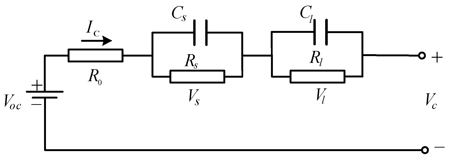
The convergence and accuracy of the battery SOC estimation are largely reliant on the exact identification of the battery model. The mainstream equivalent circuit models (ECMs) include the Rint model, R-C model, PNGV model and Thevenin model [28]. Considering the relationship between estimation accuracy, model complexity and battery dynamic characteristics, the second-order R-C network model was selected to represent the ECM used in this work, as shown in Figure 1.
where represents the terminal voltage of the battery, is the open circuit voltage (OCV), denotes the battery’s load current during charging and discharging, represents the Ohm internal resistance, the capacitive resistance branch composed of and represents the concentration polarization of the battery, whereas the other branch composed of and denotes electrochemical polarization, and and are the short-time and long-time transient voltage responses of the battery, respectively.
According to the second-order R-C network model, the battery’s discrete state space equation can be established as
where represents the SOC estimation value, is battery capacity, and is the sampling interval.
2.1. Relationship between SOC and OCV
The accuracy of SOC estimation is affected by many factors such as temperature [29], cells balancing [30,31] and OCV value [27]. In this work, considering the complexity of the model and the limitations of the experimental condition, only SOC is regarded as a non-linear function of OCV. To obtain this nonlinear function, the OCV test was conducted using a 1.6 Ah lithium battery as a case study. The test temperature was maintained at the nominal temperature (25 °C), then the lithium battery was discharged with a 0.2 C constant current. When the battery discharged 10% of its rated capacity, we stopped the discharge process and let it stand for 30 min, then we cycled the process until the discharge was completed. This is recorded in Table 1.
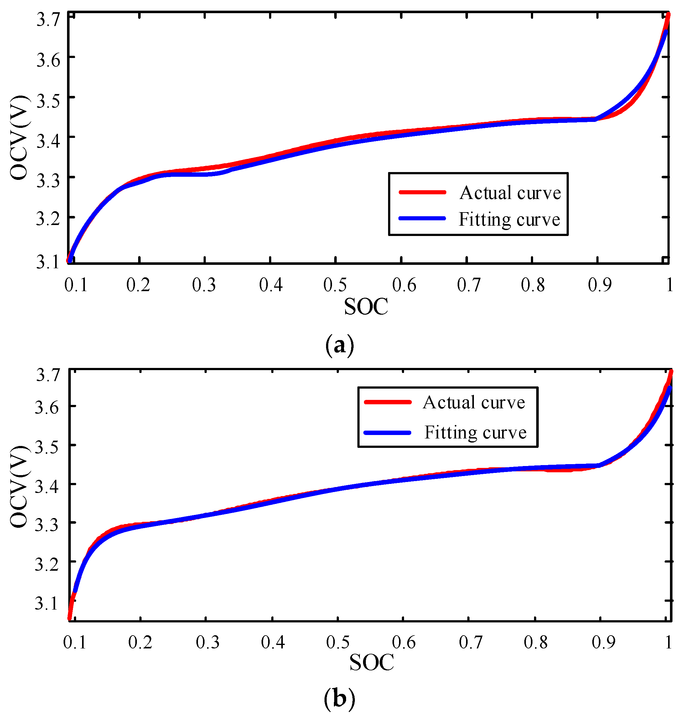
In order to more accurately establish the SOC–OCV relationship, in this experiment, the data in Table 1 are fitted in the form of a sixth polynomial plus logarithm by using the lsqcurvefit function in the MATLAB software, and compared with the eighth-order polynomial fitting implementation used in [32]. The fitting results are shown in Figure 2. Meanwhile, the standard deviation (STD) and goodness of fit (R-square) are utilized to analyze the fitting results, as shown in Table 2. The corresponding results in Table 2 and Figure 2 show that the fitting effect of the sixth-order polynomial plus logarithmic term applied in this paper is better than that of the eighth-order polynomial fitting. Hence, the nonlinear expression of SOC–OCV can be expressed as
2.2. Model Parameter Identification
It is necessary to perform parameter identification of the relevant variables in the ECM of the battery when the SOC estimation is conducted. Here, the lithium battery pulse discharge test was implemented to study the battery’s dynamic impedance characteristics under different pulse current conditions.
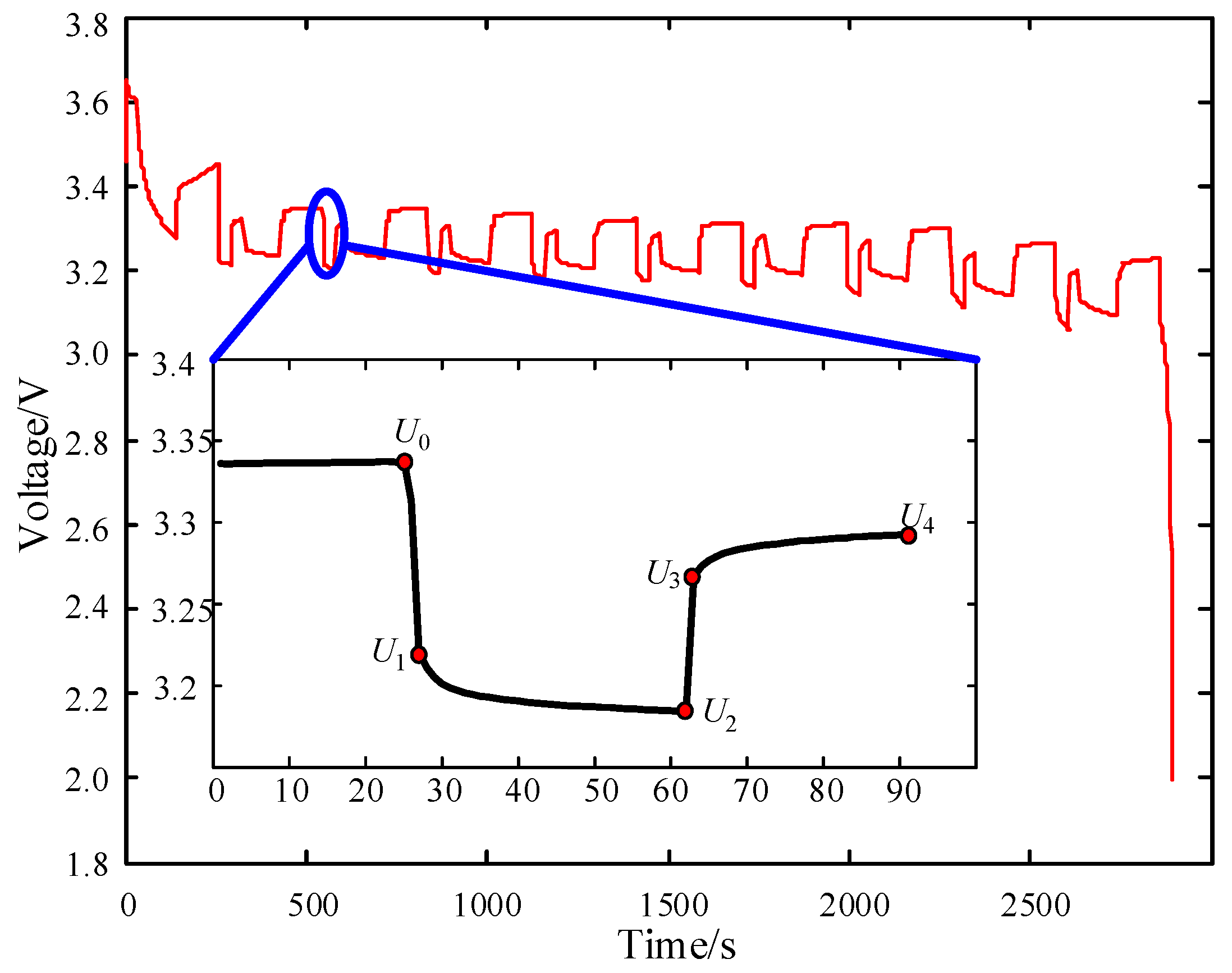
Figure 3 presents the battery’s voltage response at SOC = 1. Through the excitation response analysis of the experimental data, the least squares (LS) method is utilized to identify the parameters of the ECM under different SOCs.
According to the experimental data, the voltage changes under pulse currents can be divided into four stages: discharge (), discharge stop (), charge () and charge stop (). According to Ohm’s law of battery Ohmic resistance , the battery charge resistance can be computed as .
During the charge or discharge stop phase, due to the action of and , the change of the circuit voltage can be regarded as a zero-input response process, and the loop voltage can be expressed as
The LS fitting technique is applied to identify , the results are shown in Table 3.
2.3. Parameter Identification Result Verification
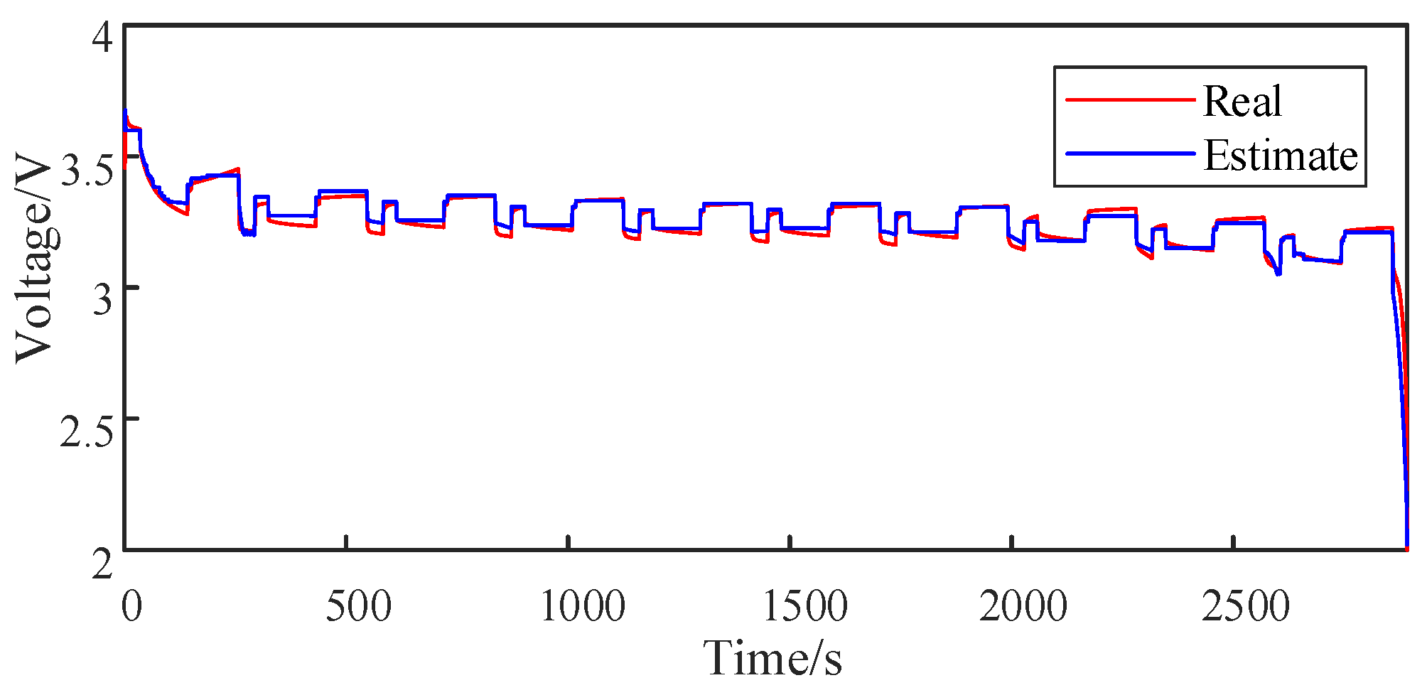
As aforementioned, the accuracy of SOC estimation largely depends on the accuracy of the initial parameter identification. Therefore, it is necessary to perform rationality verification on the identification results. The model output can be obtained as
Putting the initial parameters obtained by identification into (5), the result is shown in Figure 4, in which the red line represents the measured voltage, and the blue represents the model output value. It can be seen from Figure 4 that the blue line basically coincides with the red line, which also means that the parameters obtained above are valid.
3. SOC Estimation Based on EKF with Correntropy
In this section, we focus on the development of C-EKF and C-WLS-EKF. Considering the battery’s nonlinear characteristics, a linear state equation and a nonlinear measurement equation are used to represent the battery state.
where and are the state variable and output variable, and and denote the process noise and measurement noise; where represents the covariance of , represents the covariance of , F and B are the state transition coefficient matrix and the gain matrix, respectively, is the model input matrix, and denotes the measurement model.
The main difference between EKF and KF is that EKF uses a Jacobian matrix to transform nonlinear equations into linear equations, which can be obtained as
Therefore, the new measurement equation can be written as
Although the EKF has been extensively used for SOC estimation due to its ease of implementation [33,34,35], it still has some flaws such as the filter instability due to the Jacobian matrix [36]. Meanwhile, as pointed out in [37], the EKF is optimal under Gaussian noise conditions. However, in the case of non-Gaussian noise, the model only considers second-order moment information, so its filter is a suboptimal estimate. Therefore, a robust SOC estimation scheme via the C-EKF based on MCC with higher-order information will be developed to achieve better stability and accuracy, and we first review the correntropy in the following subsection.
3.1. Correntropy
Correntropy, as a measure of local similarity that is insensitive to outliers and noise, has been successfully applied in fields such as pattern recognition [38], machine learning [39] and signal processing [40]. Correntropy [22,41,42,43] can be expressed as follows
where X and Y represent random variables, is the expectation operator, denotes a kernel function with kernel width , and is the joint density function of X and Y. Generally, is not obtained in practice and the available samples are limited [22,44]. Hence, the sample estimator of the correntropy is recorded as
The Gaussian kernel function is utilized as the kernel function of correntropy in this paper, Hence, (11) can be rewritten as
We can observe from (12) that the correntropy takes the maximum value when X = Y, which is similar with the minimum error in MSE. Therefore, this paper uses correntropy loss instead of MSE loss to develop a more robust estimation method.
3.2. EKF with Correntropy
In this section, the C-EKF filter is mainly introduced by using the concept of correntropy as the loss function in traditional EKF.
Combining (9) and (12), a new loss function is defined as
By calculating the partial derivative of the objective function with respect to the state variable and setting it equal to zero, we obtain
Then, we can from (14) get the state update equation as
In the above formula, this paper assumes that , so then can be derived from (6), and we bring it into the denominator part of (15):
where
In the follow-up work of this section, this paper will continue to derive on the basis of (15)–(17). Under the assumption , (15) can be represented as
Then, to further introduce the measurement error term, we correct the right side of (18) by factor as
Now, we have
Both sides of (20) are divided by , so we get
where
To this end, the C-EKF can be summarized in Table 4.
3.3. C-EKF with WLS
As with the traditional EKF, the noise covariance has an impact on the performance of the C-EKF. To further improve the efficiency of the C-EKF, this paper will combine WLS with correntropy to design a more robust filter. Correntropy is used to extract high-order statistical information of an SOC estimation and introduce covariances and through WLS to minimize the variance estimation. Therefore, the new loss function can be expressed as
Computing the partial derivative of the with respect to the state variable and setting it to zero, we have the following:
Then, after some simplification of (24), we obtain
where
Adding and subtracting on the right side of (25) yields
Then, the iterative equation can be written as
where
In the new algorithm, the noise covariance existing in Equations (27) and (29) will affect the gain of the system. Finally, the filter, called C-WLS-EKF, uses the correntropy to process the non-Gaussian properties of the data and enhance the digital stability by using WLS, which is summarized in Table 5.
3.4. Convergence Analysis of the C-WLS-EKF Algorithm
The Cramér–Rao low bound criterion (CRLB) is usually utilized to verify the convergence of a novel adaptive filtering algorithm [45]. To show the effectiveness of the proposed algorithm theoretically, the CRLB of the proposed C-WLS-EKF algorithm will be derived under nonlinear conditions. Here, we define
where represents the output of the measurement equation.
The CRLB can be used to evaluate the performance of the filter and ensure the estimation accuracy of the state variable .
According to Van Trees, the amount of Fisher information in an unknown state can be expressed by
where is the conditional function of for .
For non-Gaussian noise, can be expressed as [46]
where represent the variance of Gaussian noise and short noise, respectively.
Taking the logarithm of (35):
Then, bringing into (33), we can obtain the following
This paper addresses the problem that the oscillating system is not suitable for evaluation by using the average of Fisher’s information as
If the process is ergodic, we usually think that the phase space average is equal to the time average, then
According to the definitions of global Lyapunov functions, (39) can be expressed as
When the system has chaotic characteristics, the Lyapunov functions define its parameter as a positive number. From (40), we have
According to the result of (41), one can know that the function (40) is convergence, that is, the derived C-WLS-EKF algorithm will converge to an optimal.
4. Experimental Results
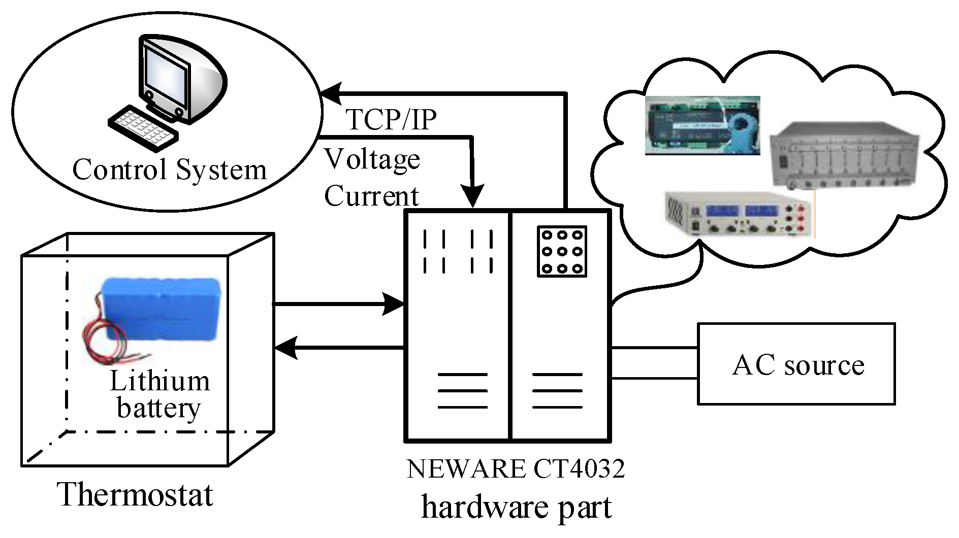
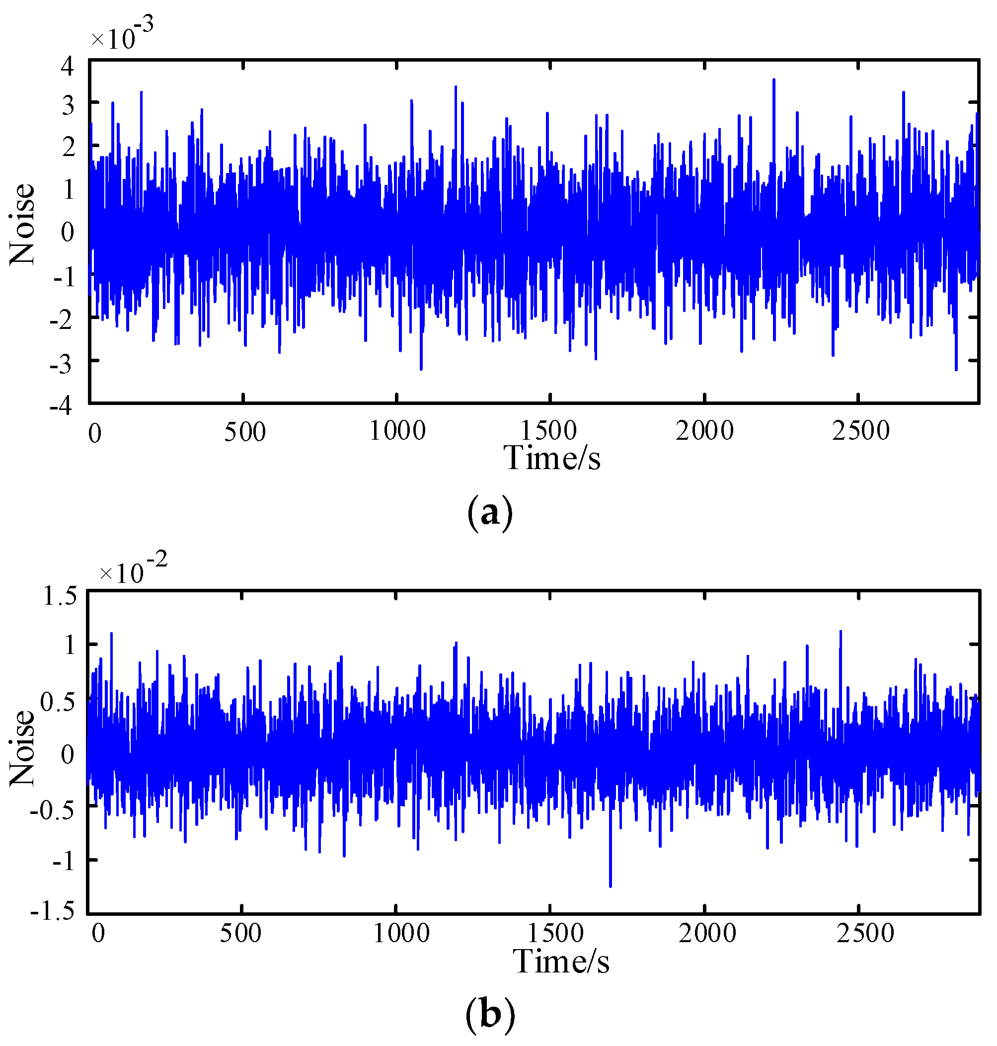
In this section, four sets of simulations are implemented to evaluate the SOC estimation performance of the C-EKF and C-WLS-EKF methods under non-Gaussian noise conditions. The schematic diagram of the lithium battery discharge test system is given in Figure 5. It mainly includes three parts, the first part is the control system which plays the information interaction role, the second is the lithium battery and Thermostat (control temperature and humidity) and the third is the hardware part of the lithium battery charge and discharge test system, which is mainly composed of a signal acquisition unit, regulated power supply, charge and discharge instrument and current transformer. In the following experiments, the original experiment data set is obtained from the lithium battery test system above. Meanwhile, all simulations are implemented on a desktop computer configured with an Intel(R) Core (TM)i5-7400 CPU. To show the robustness of the proposed method, the elements of process noise vector , along with the elements of the measurement noise , are comprised of Gaussian noise and short noise. Figure 6 shows the non-Gaussian noise applied to the experiment.
Then, the non-Gaussian mixture noise can be expressed by
From Section 3 above, one can observe that the EKF based on correntropy loss will introduce a kernel width , the value of which will affect the SOC estimation accuracy to a certain extent. In order to effectively improve the accuracy of SOC estimation, the appropriate kernel width should be selected first, and hence the influence of for the proposed method is simulated and analyzed.
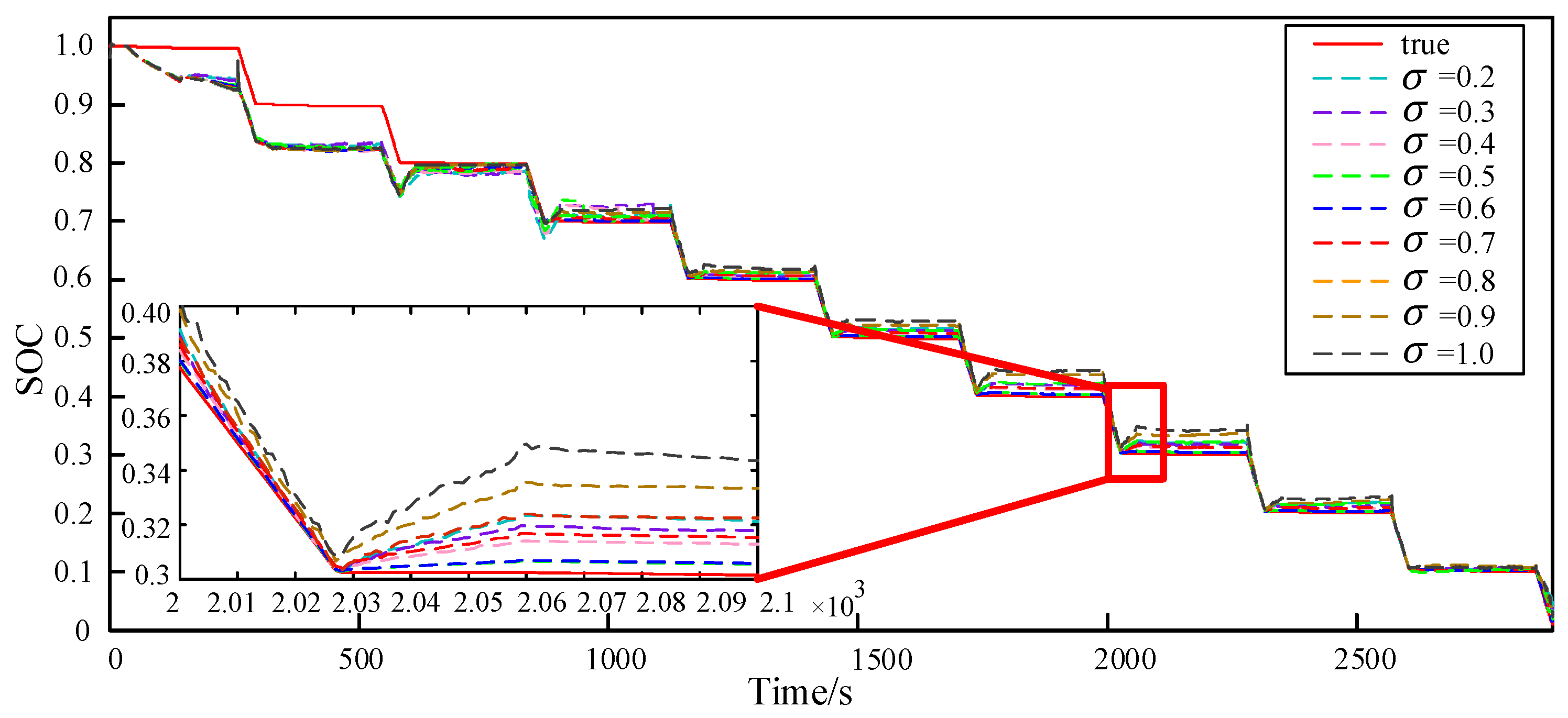
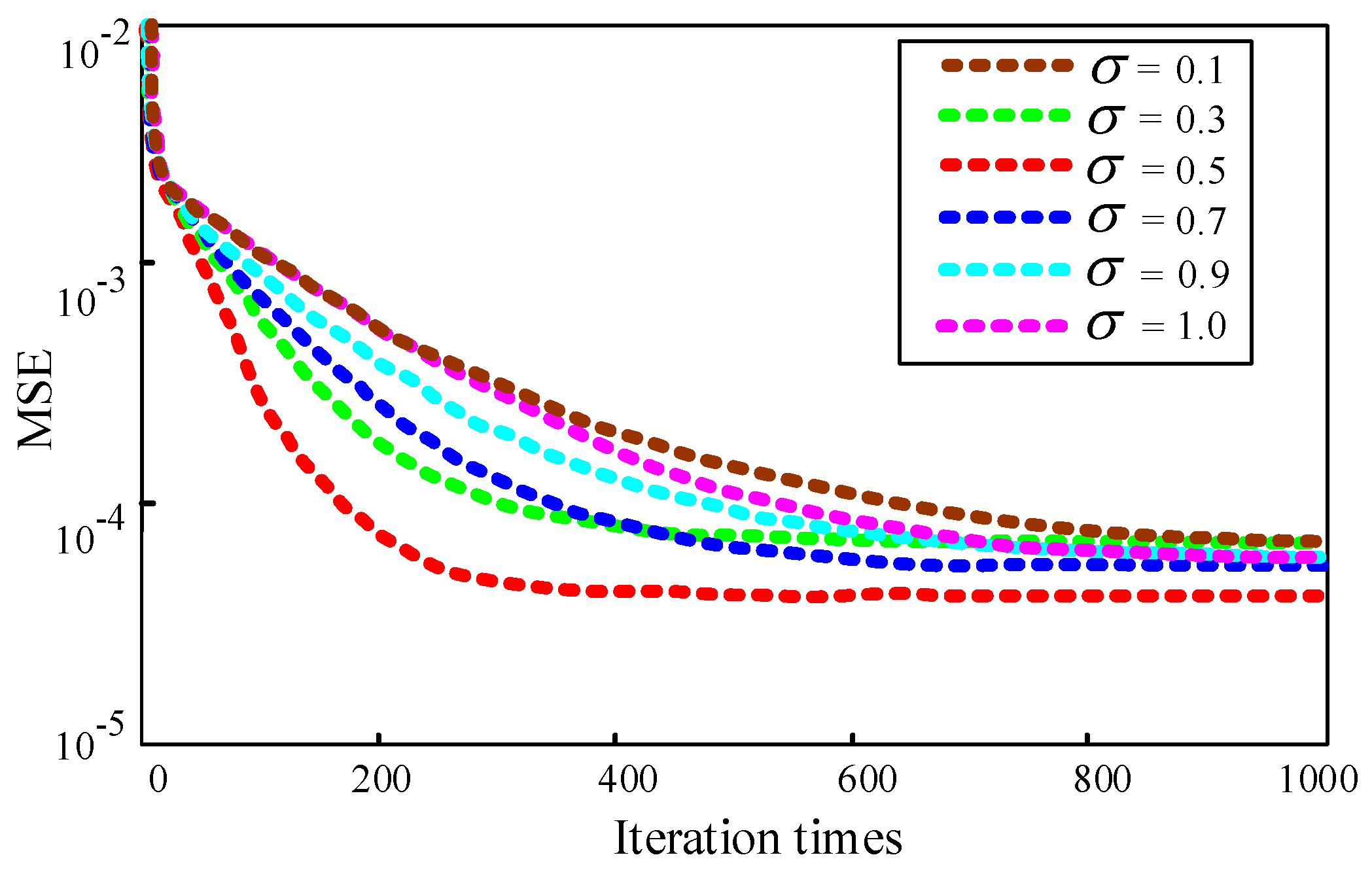
Firstly, we conduct experiments to investigate the effect of the accuracy of the proposed for the C-WLS-EKF method to further obtain an optimal kernel width for the remaining experiments. Here, the initial SOC value is set at 1, and all the parameters except remain unchanged. The SOC estimation results under different kernel widths are shown in Figure 7, where one can clearly observe through the partial enlarged view that the SOC estimation accuracy changes with the change of the kernel width . In addition, to more intuitively understand the change trend, we conduct 10 independent trails to obtain the average of the estimate errors as shown in Table 6. One can know from the corresponding results that the estimated performance is the best when . Moreover, the kernel width not only affects the estimation accuracy, but also affects the convergence performance of the algorithm. Figure 8 gives the convergence curves of the algorithm when the kernel width is set at different values. It can be seen from Figure 8 that there are significant differences in the convergence speed of the algorithm when the kernel width is set at different values. When the kernel function is taken as 0.5, the convergence rate of the algorithm is the fastest and the steady-state performance is the highest. Hence, all the kernel widths are taken as 0.5 in this study.
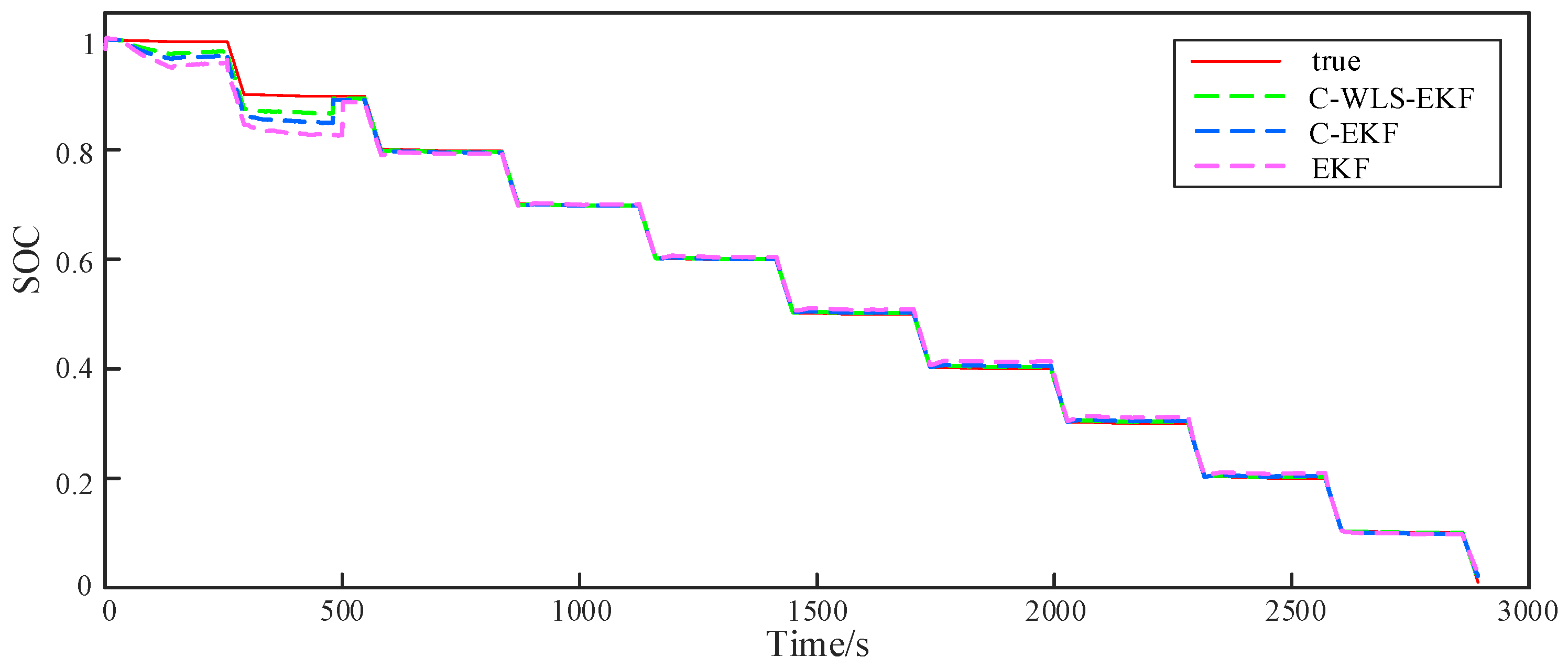
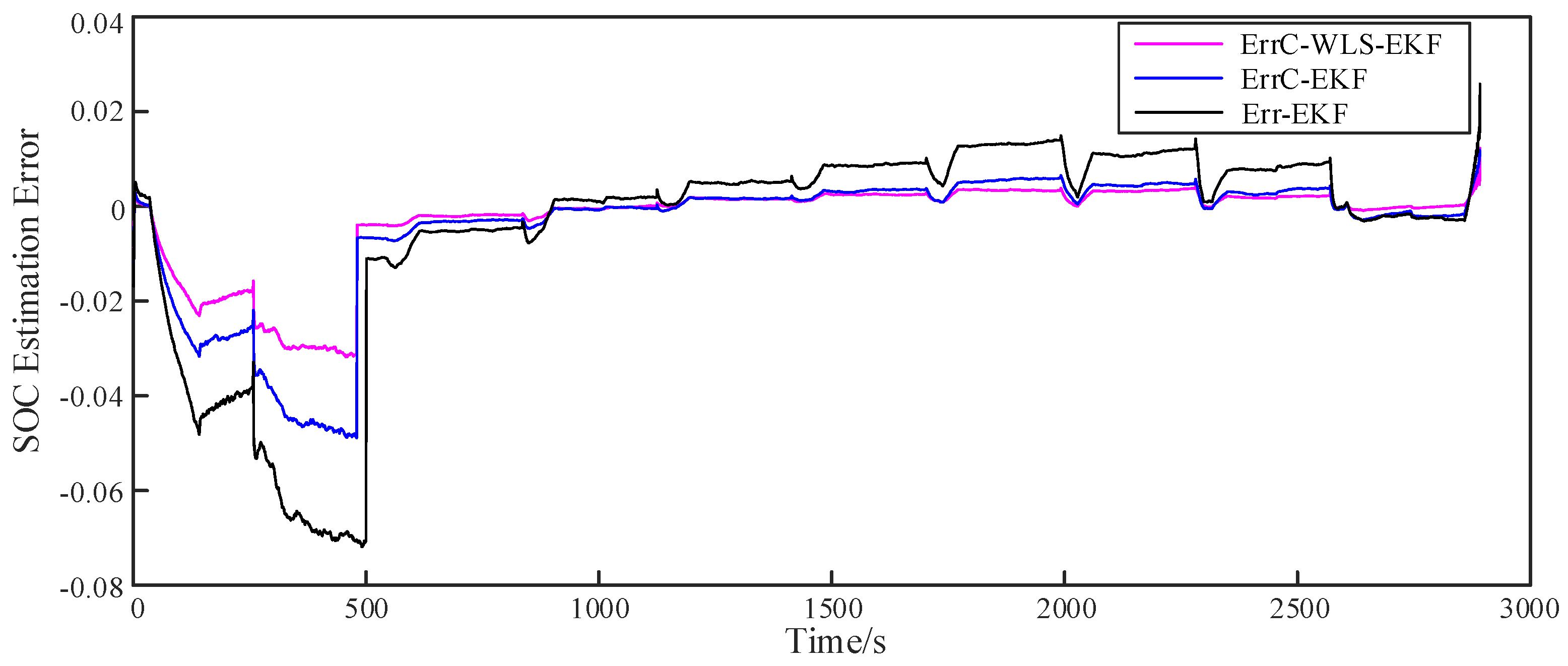
Subsequently, the estimation performance comparison experiment between the proposed method and the traditional EKF method was performed. The SOC estimation results and the error curves are shown in Figure 9 and Figure 10, respectively, in which the red line is the experimental data and other lines represent the simulation results. The vertical axis represents the SOC values from 0 to 100%. The horizontal axis represents the simulation time. The battery was discharged by withdrawing a total capacity of 1 C-rate at constant current. One can observe from the simulation results in Figure 9 and Figure 10 that (1) the estimation accuracy is low in the first 500 s because both the EKF and the improved EKF algorithm require a certain convergence time. However, the improved C-EKF and C-WLS-EKF algorithm have a faster convergence speed; (2) after 500 s, all aforementioned algorithms can effectively estimate the SOC; (3) the improved C-WLS-EKF algorithm achieves better estimation accuracy than the traditional EKF and improved C-EKF algorithms under non-Gaussian noise conditions. In addition, to quantitatively compare the performance of each algorithm, the estimation errors and CPU run time of the three algorithms are given in Table 7. According to this result in Table 7, one can know that (1) the estimated error of C-WLS-EKF achieves 0.512%, which is lower than the estimated error of the C-EKF (0.771%) and the estimated error of the EKF (1.361%). Therefore, one can be concluded that the proposed C-WLS-EKF algorithm is effective for SOC estimation under non-Gaussian noise; (2) the proposed C-EKF and C-WLS-EKF algorithms only took a little more run time from the MCC optimization in comparison to the traditional EKF, while the higher estimation precision in this case can be obtained.
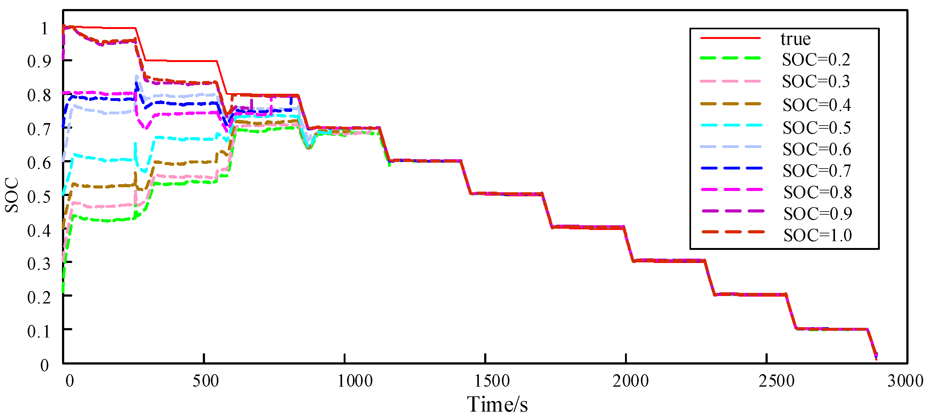
Next, this paper investigates the influence of the SOC initial value on the tracking performance of the proposed algorithm. Keeping other parameters unchanged, the initial value range of SOC is set to [0.2,1], and the experiment result is shown in Figure 11. It can be seen from Figure 11 that as the initialization value decreases, the proposed algorithm requires more iteration time to track the actual state of the battery, which also means that the convergence speed of the algorithm decreases and the estimation error increases. At the same time, it can be observed that the proposed algorithm can achieve an effective estimation after a certain time of convergence.
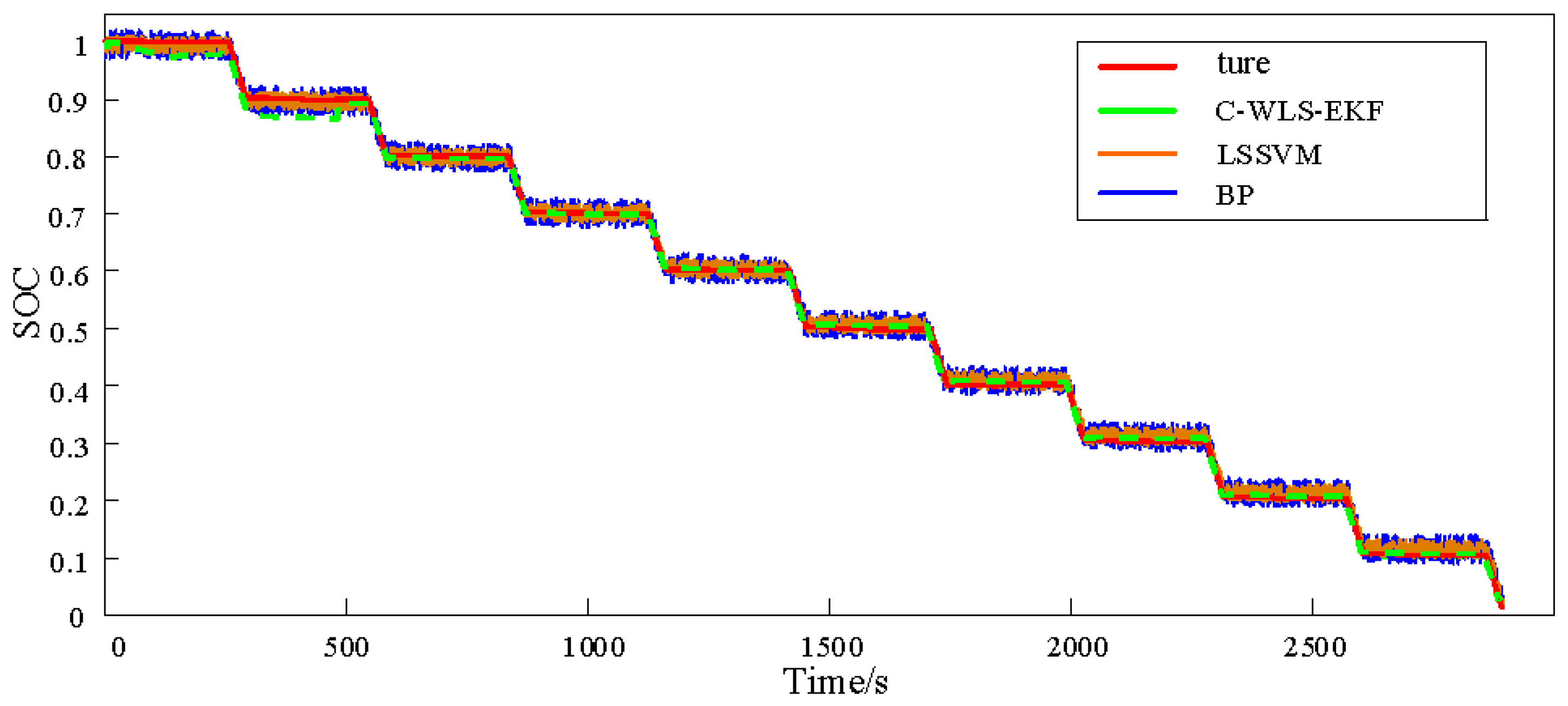
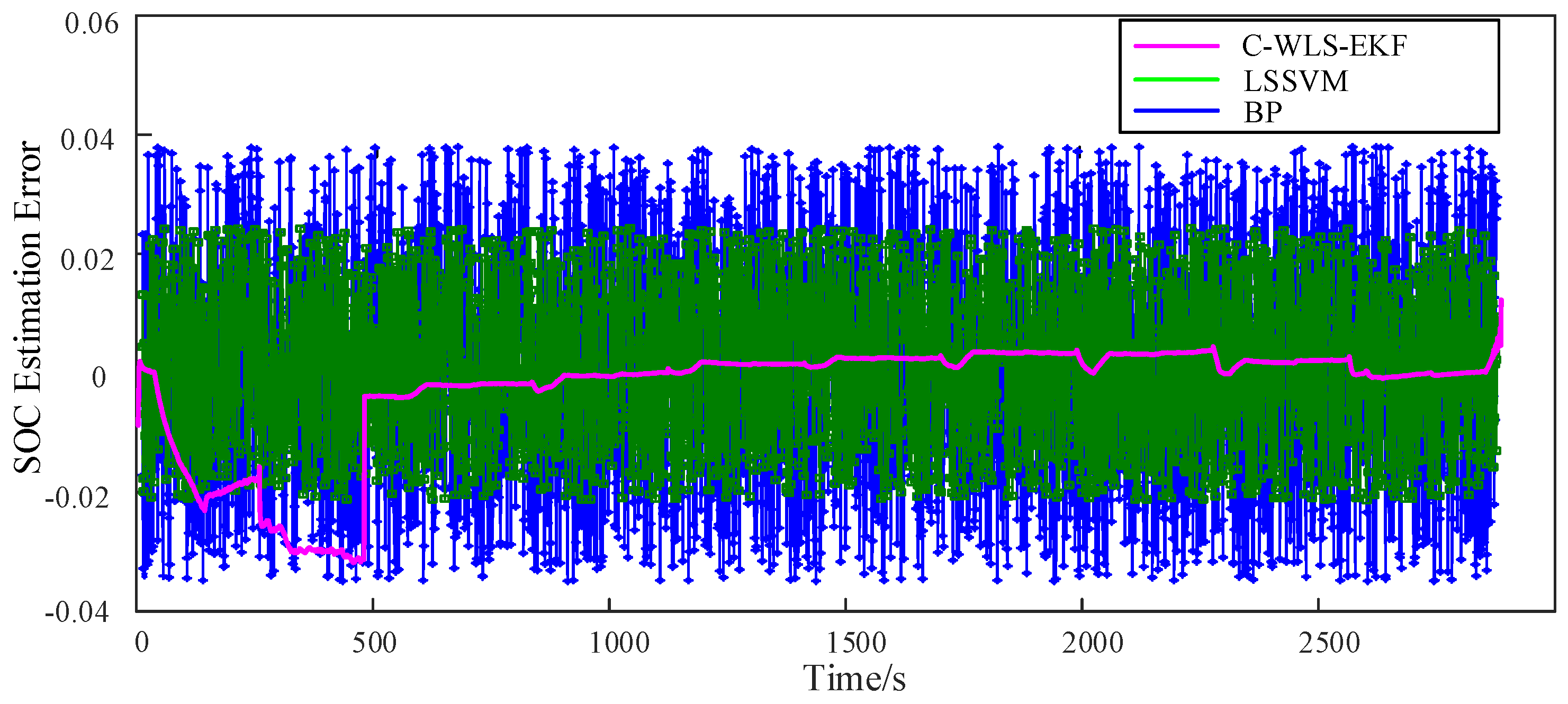
Finally, in order to evaluate the performance of the proposed C-WLS-EKF algorithm, we further conduct a comparative experiment with the data-driven methods (least squares support vector machine (LSSVM) and BP neural network). One can see from Figure 12 that the improved C-WLS-EKF algorithm in this paper has much higher accuracy than the intelligent algorithm. After calculation, the estimation errors of SOC using LSSVM and the BP neural network are 1.84% and 2.49%, respectively, which are higher than the proposed algorithms in this paper. At the same time, for a more intuitive analysis, the SOC estimation error is presented in Figure 13. Moreover, it is worth mentioning that the time complexity of the data-driven methods such as LSSVM and the BP neural network is higher than the proposed C-WLS-EKF-based SOC estimation method.
5. Conclusions
Two robust SOC estimation methods are introduced in this paper to solve the instability problem of the classic EKF method in the scenario where the system is affected by non-Gaussian noise. Firstly, this paper introduces the establishment process of the C-EKF and effectively solves the problem of SOC estimation under non-Gaussian noise. Secondly, the noise covariance is introduced into the C-EKF model by WLS, then the C-WLS-EKF model is established, and the digital stability and performance of the algorithm are effectively improved by the novel model. Finally, the CRLB criterion is utilized to verify the convergence of the C-WLS-EKF algorithm. The experimental results clarify that the performance of the proposed method under non-Gaussian noise conditions is better than traditional EKF, and the digital stability is effectively improved.
In the future, there are several interesting works that can be further conducted, such as parameters identification based on the robust online method, robust particle filter based on correntropy for SOC estimation, and so on.
Author Contributions
Conceptualization, J.D.; methodology, P.W. and W.M.; validation, X.Q., P.W., X.T., and S.F.; investigation, W.M.; data curation, P.W., X.Q.; writing—original draft preparation, P.W.; writing—review and editing, W.M.; supervision, J.D. and W.M. All authors have read and agreed to the published version of the manuscript.
Funding
This research was funded by the National Natural Science Foundation of China (51877174, 61976175), the Key Project of Natural Science Basic Research Plan in Shaanxi Province of China (2019JZ-05), the National Key R&D Program of China (2016YFB0901900), the Science and Technology Plan Project of Xi’an (GXYD14.23), and the Opening Project of State Key Laboratory of Electrical Insulation and Power Equipment (EIPE18201).
Acknowledgments
This work was supported by the National Natural Science Foundation of China (51877174, 61976175), the Key Project of Natural Science Basic Research Plan in Shaanxi Province of China (2019JZ-05), the National Key R&D Program of China (2016YFB0901900), the Science and Technology Plan Project of Xi’an (GXYD14.23), and the Opening Project of State Key Laboratory of Electrical Insulation and Power Equipment (EIPE18201).
Conflicts of Interest
The authors declare no conflicts of interest.
References
- Hannan, M.A.; Hoque, M.M.; Peng, S.E.; Uddin, M.N. Lithium-ion battery charge equalization algorithm for electric vehicle applications. IEEE Trans. Ind. Appl. 2017, 53, 2541–2549. [Google Scholar] [CrossRef]
- Dong, G.; Chen, Z.; Wei, J. Sequential Monte Carlo filter for state of charge estimation of lithium-ion batteries based on auto regressive exogenous model. IEEE Trans Ind. Electron. 2019, 66, 8533–8544. [Google Scholar] [CrossRef]
- Wei, Z.; Leng, F.; He, Z.; Zhang, W.; Li, K. Online state of charge and state of health estimation for a Lithium-Ion battery based on a data–model fusion method. Energies 2018, 11, 1810. [Google Scholar] [CrossRef] [Green Version]
- Pan, H.; Lv, Z.; Lin, W.; Li, J.; Chen, L. State of charge estimation of lithium-ion batteries using a grey extended Kalman filter and a novel open-circuit voltage model. Energy 2017, 138, 764–775. [Google Scholar] [CrossRef]
- Ding, N.; Prasad, K.; Lie, T.T.; Cui, J. State of charge estimation of a composite lithium-based battery model based on an improved extended kalman filter algorithm. Inventions 2019, 4, 66. [Google Scholar] [CrossRef] [Green Version]
- Feng, F.; Lu, R.; Zhu, C. A combined state of charge estimation method for lithium-ion batteries used in a wide ambient temperature range. Energies 2014, 7, 1–29. [Google Scholar] [CrossRef] [Green Version]
- Dong, G.; Wei, J.; Zhang, C.; Chen, Z. Online state of charge estimation and open circuit voltage hysteresis modeling of LiFePO4 battery using invariant imbedding method. Appl. Energy 2016, 162, 163–171. [Google Scholar] [CrossRef]
- Tong, S.; Lacap, J.H.; Park, J.W. Battery state of charge estimation using a load-classifying neural network. J. Energy Storage 2016, 7, 236–243. [Google Scholar] [CrossRef]
- Yang, F.; Li, W.; Li, C.; Miao, Q. State-of-charge estimation of lithium-ion batteries based on gated recurrent neural network. Energy 2019, 175, 66–75. [Google Scholar] [CrossRef]
- Chen, B.; Xing, L.; Xu, B.; Zhao, H.; Príncipe, J.C. Insights into the robustness of minimum error entropy estimation. IEEE Trans. Neural Netw. Learn Syst. 2016, 29, 731–737. [Google Scholar] [CrossRef]
- Muhammad, S.; Rafique, M.U.; Li, S.; Shao, Z.; Wang, Q.; Guan, N. A robust algorithm for state-of-charge estimation with gain optimization. IEEE Trans. Ind. Inform. 2017, 13, 2983–2994. [Google Scholar] [CrossRef]
- Meng, J.; Stroe, D.I.; Ricco, M.; Luo, G.; Teodorescu, R. A simplified model-based state-of-charge estimation approach for lithium-ion battery with dynamic linear model. IEEE Trans. Ind. Electron. 2018, 66, 7717–7727. [Google Scholar] [CrossRef] [Green Version]
- Li, Y.; Chen, J.; Lan, F. Enhanced online model identification and state of charge estimation for lithium-ion battery under noise corrupted measurements by bias compensation recursive least squares. J. Power Sources 2020, 456, 227984. [Google Scholar] [CrossRef]
- Zhi, L.; Peng, Z.; Zhi, W.; Qiang, S.; Yinan, R. State of charge estimation for Li-ion battery based on extended Kalman filter. Energy Procedia 2017, 105, 3515–3520. [Google Scholar] [CrossRef]
- Wang, Q.; Feng, X.; Zhang, B.; Gao, T.; Yang, Y. Power battery state of charge estimation based on extended Kalman filter. J. Renew. Sustain. Energy 2019, 11, 014302. [Google Scholar] [CrossRef]
- Baccouche, I.; Jemmali, S.; Manai, B.; Omar, N.; Amara, N. Improved OCV model of a Li-ion NMC battery for online SOC estimation using the extended Kalman filter. Energies 2017, 10, 764. [Google Scholar] [CrossRef] [Green Version]
- Yan, W.; Zhang, B.; Zhao, G.; Tang, S.; Niu, G.; Wang, X. A battery management system with a Lebesgue-sampling-based extended Kalman filter. IEEE Trans. Ind. Electron. 2018, 66, 3227–3236. [Google Scholar] [CrossRef]
- Lai, X.; Wang, S.; He, L.; Zhou, L.; Zheng, Y. A hybrid state-of-charge estimation method based on credible increment for electric vehicle applications with large sensor and model errors. J. Energy Storage 2020, 27, 101106. [Google Scholar] [CrossRef]
- Zhu, Q.; Xu, M.; Liu, W.; Zheng, M. A state of charge estimation method for lithium-ion batteries based on fractional order adaptive extended kalman filter. Energy 2019, 187, 115880. [Google Scholar] [CrossRef]
- Xiao, R.; Shen, J.; Li, X.; Yan, W.; Pan, E.; Chen, Z. Comparisons of modeling and state of charge estimation for lithium-ion battery based on fractional order and integral order methods. Energies 2016, 9, 184. [Google Scholar] [CrossRef]
- Wei, Z.; Meng, S.; Xiong, B.; Ji, D.; Tseng, K.J. Enhanced online model identification and state of charge estimation for lithium-ion battery with a FBCRLS based observer. Appl. Energy 2016, 181, 332–341. [Google Scholar] [CrossRef]
- Liu, W.; Pokharel, P.P.; Principe, J.C. Correntropy: Properties and applications in non-gaussian signal processing. IEEE Trans. Signal Process 2007, 55, 5286–5298. [Google Scholar] [CrossRef]
- Chen, B.; Liu, X.; Zhao, H.; Jose, C. Maximum correntropy Kalman filter. Automatica 2017, 76, 70–77. [Google Scholar] [CrossRef] [Green Version]
- Izanloo, R.; Fakoorian, S.A.; Yazdi, H.S.; Simon, D. Kalman filtering based on the maximum correntropy criterion in the presence of non-Gaussian noise. In Proceedings of the IEEE 2016 Annual Conference on Information Science and Systems (CISS), Princeton, NJ, USA, 16–18 March 2016; pp. 500–505. [Google Scholar]
- Mohiuddin, S.M.; Qi, J. Maximum correntropy extended Kalman filtering for power system dynamic state estimation. In Proceedings of the 2019 IEEE Power & Energy Society General Meeting (PESGM), Atlanta, GA, USA, 4–8 August 2019; pp. 1–5. [Google Scholar]
- Wang, G.; Zhang, Y.; Wang, X. Iterated maximum correntropy unscented Kalman filters for non-Gaussian systems. Signal Process 2019, 163, 87–94. [Google Scholar] [CrossRef]
- Sun, Q.; Zhang, H.; Zhang, J.; Ma, W. Adaptive unscented kalman filter with correntropy loss for robust state of charge estimation of lithium-ion battery. Energies 2018, 11, 3123. [Google Scholar] [CrossRef] [Green Version]
- Nikolian, A.; Jaguemont, J.; de Hoog, J.; Goutam, S.; Omar, N.; Van Den Bossche, P.; Van Mierlo, J. Complete cell-level lithium-ion electrical ECM model for different chemistries (NMC, LFP, LTO) and temperatures (−5 °C to 45 °C)–Optimized modelling techniques. Int. J. Electr. Power Energy Syst. 2018, 98, 133–146. [Google Scholar] [CrossRef]
- Alipour, M.; Ziebert, C.; Conte, F.V.; Kizilel, R. A review on temperature-dependent electrochemical properties, aging, and performance of lithium-ion cells. Batteries 2020, 6, 35. [Google Scholar] [CrossRef]
- Shousha, M.; Prodic, A.; Marten, V.; Milios, J. Design and implementation of assisting converter-based integrated battery management system for electromobility applications. IEEE J. Emerg. Sel. Top. Power Electron. 2017, 6, 825–842. [Google Scholar] [CrossRef]
- Shousha, M.; McRae, T.; Prodic, A.; Marten, V.; Milios, J. Design and implementation of high power density assisting step-up converter with integrated battery balancing feature. IEEE J. Emerg. Sel. Top. Power Electron. 2017, 5, 1068–1077. [Google Scholar] [CrossRef]
- Dang, X.; Yan, L.; Jiang, H.; Wu, X.; Sun, H. Open-circuit voltage-based state of charge estimation of lithium-ion power battery by combining controlled auto-regressive and moving average modeling with feedforward-feedback compensation method. Int. J. Electr. Power Energy Syst. 2017, 90, 27–36. [Google Scholar] [CrossRef]
- Pérez, G.; Garmendia, M.; Reynaud, J.F.; Crego, J.; Viscarret, U. Enhanced closed loop State of Charge estimator for lithium-ion batteries based on Extended Kalman Filter. Appl. Energy 2015, 155, 834–845. [Google Scholar] [CrossRef]
- Guo, F.; Hu, G.; Xiang, S.; Zhou, P.; Hong, R.; Xiong, N. A multi-scale parameter adaptive method for state of charge and parameter estimation of lithium-ion batteries using dual Kalman filters. Energy 2019, 178, 79–88. [Google Scholar] [CrossRef]
- Chen, B.; Wang, J.; Zhao, H.; Zheng, N.; Príncipe, J.C. Convergence of a fixed-point algorithm under maximum correntropy criterion. IEEE Signal Process Lett. 2015, 22, 1723–1727. [Google Scholar] [CrossRef]
- Liu, X.; Qu, H.; Zhao, J.; Chen, B. Extended Kalman filter under maximum correntropy criterion. In Proceedings of the 2016 International Joint Conference on Neural Networks (IJCNN), Vancouver, BC, Canada, 24–29 July 2016; pp. 1733–1737. [Google Scholar]
- Ma, W.; Qu, H.; Gui, G.; Xu, L.; Zhao, J.; Chen, B. Maximum correntropy criterion based sparse adaptive filtering algorithms for robust channel estimation under non-Gaussian environments. J. Frankl. Inst. 2015, 352, 2708–2727. [Google Scholar] [CrossRef] [Green Version]
- Chen, B.; Li, Y.; Dong, J.; Lu, N.; Qin, J. Common spatial patterns based on the quantized minimum error entropy criterion. IEEE Trans. Syst. Man Cybern. Syst. 2018, 1–12. [Google Scholar] [CrossRef]
- Duan, J.; Qiu, X.; Ma, W.; Tian, X.; Shang, D. Electricity consumption forecasting scheme via improved LSSVM with maximum correntropy criterion. Entropy 2018, 20, 112. [Google Scholar] [CrossRef] [Green Version]
- Zhao, J.; Mili, L. A framework for robust hybrid state estimation with unknown measurement noise statistics. IEEE Trans. Ind. Inform. 2017, 14, 1866–1875. [Google Scholar] [CrossRef]
- Ma, W.; Qiu, J.; Liu, X.; Xiao, G.; Duan, J.; Chen, B. Unscented kalman filter with generalized correntropy loss for robust power system forecasting-aided state estimation. IEEE Trans. Ind. Inform. 2019, 15, 6091–6100. [Google Scholar] [CrossRef]
- Ma, W.; Duan, J.; Man, W.; Zhao, H.; Chen, B. Robust kernel adaptive filters based on mean p-power error for noisy chaotic time series prediction. Eng. Appl. Artif. Intel. 2017, 58, 101–110. [Google Scholar] [CrossRef]
- Ma, W.; Duan, J.; Chen, B.; Gui, G.; Man, W. Recursive generalized maximum correntropy criterion algorithm with sparse penalty constraints for system identification. Asian J. Control. 2017, 19, 1164–1172. [Google Scholar] [CrossRef]
- Ma, W.; Qiu, X.; Duan, J.; Li, Y.; Chen, B. Kernel recursive generalized mixed norm algorithm. J. Frankl. Inst. 2018, 355, 1596–1613. [Google Scholar] [CrossRef]
- Schmitt, L.; Fichter, W. Cramér-Rao lower bound for state-constrained nonlinear filtering. IEEE Signal Process Lett. 2017, 24, 1882–1885. [Google Scholar] [CrossRef]
- Sayin, M.O.; Vanli, N.D.; Kozat, S.S. A novel family of adaptive filtering algorithms based on the logarithmic cost. IEEE Trans. Signal Process 2014, 62, 4411–4424. [Google Scholar] [CrossRef] [Green Version]
Figure 1.
Second-order R-C equivalent circuit model (ECM).

Figure 2.
SOC–OCV relationship curve: (a) 8th-order polynomial function fitting curve; (b) 6th-order polynomial plus a logarithmic term function fitting curve.
Figure 2.
SOC–OCV relationship curve: (a) 8th-order polynomial function fitting curve; (b) 6th-order polynomial plus a logarithmic term function fitting curve.

Figure 3.
Lithium battery discharge curve.

Figure 4.
Comparison of model output value with real value.

Figure 5.
Discharge testing system schematic diagram.

Figure 6.
Non-Gaussian noise schematic: (a) state noise; (b) measurement noise.

Figure 7.
SOC estimation results under different kernel widths.

Figure 8.
Convergence performance of C-WLS-EKF algorithms under different kernel widths.

Figure 9.
SOC comparison of different algorithm estimation results when the initial value of SOC = 1.
Figure 9.
SOC comparison of different algorithm estimation results when the initial value of SOC = 1.

Figure 10.
SOC estimation error curve under non-Gaussian noise.

Figure 11.
Estimated results under different initial SOCs.

Figure 12.
Comparison of C-WLS-EKF and intelligent algorithm estimation results.

Figure 13.
Estimation error distribution of the C-WLS-EKF and intelligent algorithm.


Table 1.
State of charge (SOC)–open circuit voltage (OCV) discharge measurement data.
| SOC/% | Voltage/V | SOC/% | Voltage/V |
|---|---|---|---|
| 100 | 3.635 | 50 | 3.374 |
| 90 | 3.432 | 40 | 3.340 |
| 80 | 3.429 | 30 | 3.307 |
| 70 | 3.411 | 20 | 3.281 |
| 60 | 3.402 | 10 | 3.109 |
Table 2.
Comparative analysis of fitting results.
| Index | 8th-Order | 6th-Order |
|---|---|---|
| STD | 0.0176 | 0.0059 |
| R-square | 0.0985 | 0.0998 |
Table 3.
Parameter identification results.
| Parameter | Value |
|---|---|
| 39 | |
| 2 | |
| 17.4 | |
| 7.88 | |
| 1.14 |
Table 4.
Correntropy extended Kalman filter (C-EKF).
Table 5.
C-WLS-EKF.
Table 6.
Estimation error under different kernel widths.
| 0.1 | 0.2 | 0.3 | 0.4 | 0.5 | |
|---|---|---|---|---|---|
| Estimation error (%) | 1.27 | 1.12 | 1.04 | 0.703 | 0.512 |
| 0.6 | 0.7 | 0.8 | 0.9 | 1 | |
| Estimation error (%) | 0.694 | 0.879 | 1.07 | 1.14 | 1.37 |
Table 7.
SOC estimation errors and CPU run time of different methods under non-Gaussian noise conditions.
Table 7.
SOC estimation errors and CPU run time of different methods under non-Gaussian noise conditions.
| Algorithm | C-WLS-EKF | C-EKF | EKF |
|---|---|---|---|
| Estimation error (%) | 0.512 | 0.771 | 1.361 |
| t(s) | 9.71 | 9.26 | 8.89 |
© 2020 by the authors. Licensee MDPI, Basel, Switzerland. This article is an open access article distributed under the terms and conditions of the Creative Commons Attribution (CC BY) license (http://creativecommons.org/licenses/by/4.0/).
Share and Cite
MDPI and ACS Style
Duan, J.; Wang, P.; Ma, W.; Qiu, X.; Tian, X.; Fang, S. State of Charge Estimation of Lithium Battery Based on Improved Correntropy Extended Kalman Filter. Energies 2020, 13, 4197. https://0-doi-org.brum.beds.ac.uk/10.3390/en13164197
AMA Style
Duan J, Wang P, Ma W, Qiu X, Tian X, Fang S. State of Charge Estimation of Lithium Battery Based on Improved Correntropy Extended Kalman Filter. Energies. 2020; 13(16):4197. https://0-doi-org.brum.beds.ac.uk/10.3390/en13164197
Chicago/Turabian StyleDuan, Jiandong, Peng Wang, Wentao Ma, Xinyu Qiu, Xuan Tian, and Shuai Fang. 2020. "State of Charge Estimation of Lithium Battery Based on Improved Correntropy Extended Kalman Filter" Energies 13, no. 16: 4197. https://0-doi-org.brum.beds.ac.uk/10.3390/en13164197
Note that from the first issue of 2016, this journal uses article numbers instead of page numbers. See further details here.