An Ultra-Short-Term Electrical Load Forecasting Method Based on Temperature-Factor-Weight and LSTM Model

Abstract

Ultra-short-term electrical load forecasting is an important guarantee for the safety and efficiency of energy system operation. Temperature is also an important factor affecting the changes in electric load. However, in different cases, the impact of temperature on load forecasting will vary greatly, and sometimes even lead to the decrease of forecasting accuracy. This often brings great difficulties to researchers’ work. In order to make more scientific use of temperature factor for ultra-short-term electrical load forecasting, especially to avoid the negative influence of temperature on load forecasting, in this paper we propose an ultra-short-term electrical load forecasting method based on temperature factor weight and long short-term memory model. The proposed method evaluates the importance of the current prediction task’s temperature based on the change magnitude of the recent load and the correlation between temperature and load, and therefore the negative impacts of the temperature model can be avoided. The mean absolute percentage error of proposed method is decreased by 1.24%, 1.86%, and 6.21% compared with traditional long short-term memory model, back-propagation neural network, and gray model on average, respectively. The experimental results demonstrate that this method has obvious advantages in prediction accuracy and generalization ability.

1. Introduction

Ultra-short-term electrical load forecasting (USTLF), which refers to the forecasting of the load within one day [1], is the basis of safety, reliability, and economy of energy system operation. Owing to the increasing demand of distributed energy and various users, the randomness of load changes increases the difficulty associated with load forecasting. USTLF provides a basis for determining trends in the electricity market price [2]. Too large a prediction error will result in higher operating costs.

There are many load forecasting methods utilized at present. Zhengyuan et al. [3] proposed an original data sequence by third parties for the opening sequence of operations to generate new data. Furthermore, it can be used to establish an improved GM (1,1) model. Song et al. [4] built a combined model based on the BP network model and GM (1,1) residual correction, designed to improve the precision of load forecasting models. Liu et al. [5] introduced the idea of fractional order accumulation into the GM (1,1) model, then improved the traditional BP neural network through the use of the layered training algorithm. Long et al. [6] devised a monthly power load combination prediction model based on seasonal adjustment method and the BP neural network. Moreover, Ge et al. [7] developed a power load prediction algorithm based on fuzzy BP-NNs and a combined adaptive cubature Kalman filter. Hu [8] proposed a GM (1,1) model based on neural network to solve the problem of the development coefficient and control variables being dependent on the fluctuating background value in the traditional gray prediction model. Rim et al. [9] built an artificial neural networks to predict the half-hourly electric load demand in Tunisia over the period from 2000 to 2008. Behm et al. [10] developed a methodology to provide weather-dependent countrywide electricity load profiles using artificial neural networks. The method could be used as a basis for much needed long-term load predictions for European countries. Pal et al. [11] proposed a hybridized forecasting model based on weight adjustment of neural networks with BP learning using general type-2 fuzzy sets. Parvez et al. [12] proposed a Multilayer Perceptron (MLP)-based photo voltaic forecasting method for the rooftop photovoltaic systems of the smart home. Currently, with the rapid development of the deep learning [13,14,15,16,17], various deep neural network models, specially LSTM and its variants, are widely employed in the load forecasting tasks. Hochreiter et al. [18] proposed a LSTM model, which added several control gates to the traditional recurrent neural network (RNN) for processing of long-term dependencies in timing problems. Shahzad et al. [19] used long-short-term memory artificial neural networks to predict the power load in different time periods. Santra et al. [20] utilized LSTM and GA to increase the robustness of short-term load forecasting. For their part, Qing et al. [21] proposed an hourly solar radiation intensity prediction method based on weather forecast data; moreover, Li [22] employed a deep learning LSTM circulating neural network algorithm based on the TensorFlow intelligent learning system for short-term power load prediction purposes. Chen et al. [23] combined the LSTM forecasting model with the XGBoost forecasting model to achieve power load forecasting. Zhang et al. [24] developed a LSTM network model scheme suitable for power load forecasting in Yichang. Liu et al. [25] proposed a stacked denoising autoencoder model for short-term load forecasting. In addition, some researchers have applied a third-generation artificial neural network, the spiking neural network, to power load forecasting [26,27,28].

Ambient temperature is one of the important factors that impact changes in electric load [29]. For example, scorching heat will bring an increase in air conditioning load. However, when the scope of the research is extended to the general case, temperature analysis does not necessarily improve prediction accuracy. In fact, when the correlation between temperature and load is weak, temperature analysis can even decrease the load prediction accuracy. In some relatively stable load cases, the influence of temperature on load has been included in the recent historical data. Even if a strong correlation exists between temperature and load, higher accuracy can be achieved if temperature is not considered. In the present study [30,31], the researchers simply considered the correlation between temperature and load in load forecasting; no further assessment of the impact of temperature on the model was conducted. In order to make better use of the temperature factor, we propose a method that combines the temperature factor weight (TFW) and the Long short-term memory (LSTM) model (TFW-LSTM). By analyzing the historical load data and historical temperature data in the current prediction task, the module feeds back the TFW value which determines whether the system needs to consider the temperature factor. Therefore, the TFW-LSTM method can improve the forecasting accuracy of power load, which is beneficial to the utilization rate of power generation equipment and the effectiveness of economic dispatching.

Section 2 chiefly describes the basic principle of LSTM artificial neural networks, while Section 3 describes the TFW-LSTM method in more detail. Section 4 mainly presents the experimental results and the discussion thereof. Finally, Section 5 outlines the conclusion.

2. Long Short-Term Memory Artificial Neural Networks

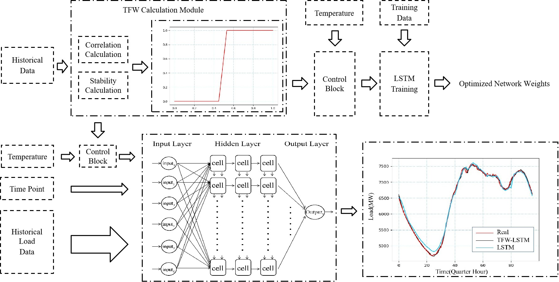
LSTM artificial neural networks are a special type of recurrent neural network (RNN). LSTM mainly solves the phenomenon of “gradient explosion” or “gradient disappearance” in the RNN context, making them better able to deal with the problem of long-distance dependence. A multilayer LSTM network structure model is shown in Figure 1.

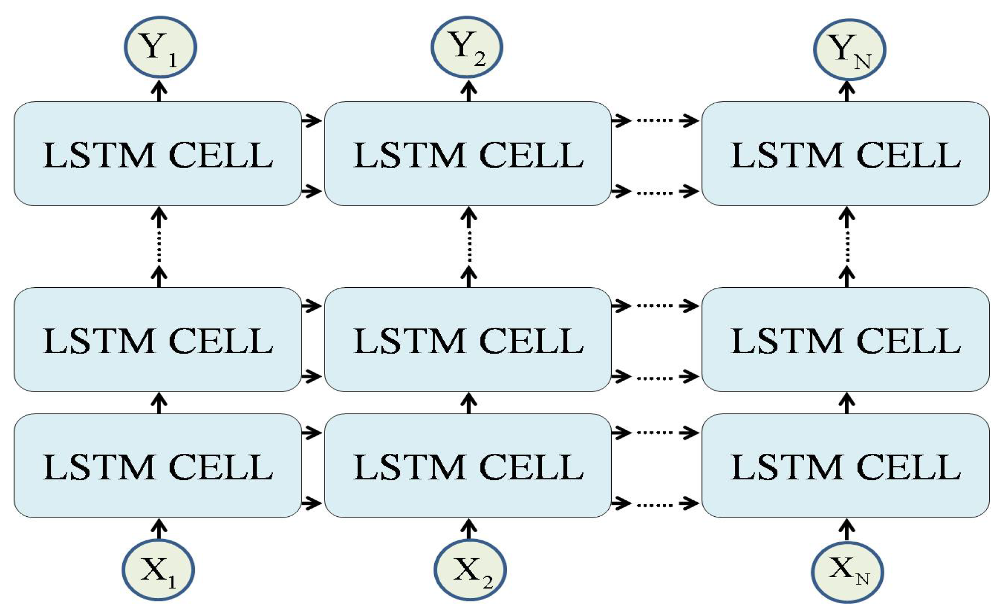
The construction of the LSTM network unit is depicted in Figure 2. Here, C represents the long-term memory of LSTM, which adds new memory in real-time as the network operates. The $h_{t-1}$ denotes the output from the previous point in time, while $h_t$ is the output at the current point in time. Moreover, $X_t$ represents the current input. The internal function modules of the LSTM unit will be introduced below.

• Forget gate: The forget gate determines by the forgetting coefficient, which refers to how much of the long-term memory $C_{t-1}$ of the previous moment should be retained. It further integrates the output $h_{t-1}$ of the previous time point with the input $X_t$ of the current time point into an input matrix $[h_{t-1},X_t]$. Finally, the sigmoid activation function outputs a real number in the range (0,1); here, 1 means that all memories should be stored, while 0 indicates that all memories should be forgotten:

  $$f_t=\sigma (W_f·[h_{t-1},x_t]+b_f)$$

  (1)

  Here, $\sigma$ is the activation function, $W_f$ represents the weight matrix of the fully connected layer network, and $b_f$ indicates the bias matrix of the fully connected layer network; moreover, $f_t$ is the forgetting coefficient.
• Input gate: Function of the input gate: it determines how much of the current input $X_t$ is saved for long-term memory $C_t$:

  $$\left\{\begin{array}{c}{i}_t=\sigma (W_i·[h_{t-1},x_t]+b_i)\hfill \\ \widetilde{C_t}=tanh(W_C·[h_{t-1},x_t]+b_C)\hfill \end{array}\right.$$

  (2)

  Here, $W_i$ and $b_i$ denote the weight and bias parameters, respectively, of the function sigmoid at the fully connection layer, while $W_c$ and $b_C$ are the weight and bias parameters, respectively, of the tanh function of the fully connection layer.
• Output gate: Function of the output gate: the intermediate parameter $o_t$ is used to determine the extent to which the long-term memory $C_t$ affects the current cell output:

  $$\left\{\begin{array}{c}{o}_t=\sigma (W_o·[h_{t-1},x_t]+b_o)\hfill \\ h_t=o_t·tanh\left(C_t\right)\hfill \end{array}\right.$$

  (3)

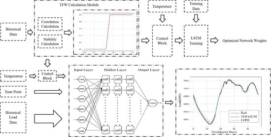
3. TFW-LSTM Method

The traditional USTLF method is not sufficiently comprehensive when temperature is considered. When the correlation between the temperature and power load is strong, temperature can improve the precision of power load prediction; when this correlation is weak, however, this precision will decrease. Similarly, load forecasting that does not consider temperature can in fact achieve higher prediction accuracy, provided that the recent load is stable enough. In order to make better use of the temperature information, we propose an USTLF method that combines TFW and the LSTM model to solve the above problems. Accordingly, we add a TFW calculation module to the LSTM neural network based load forecasting method. After analyzing the historical load and temperature data in the current prediction task, the module feeds back the TFW value which determines whether the system needs to consider the temperature.

3.1. Data Acquisition and Preprocessing

We use the electrical load and temperature data of a city in Hunan province in 2019. The temporal resolution of the load data provided by the power company is 15 min, while the weather data was obtained from an open source weather (website Available: http://www.tianqihoubao.com/lishi/changsha.html) using a web crawler. It is determined that the original electric load data cannot be used directly in the present experiment; there are some missing data, which are marked by the power company using the value −999. Therefore, some missing data are simulated and filled according to the changing trends of the data across time. To accomplish this, a data filling algorithm is proposed to fill in the missing data values so that they are as close as possible to the real values. This filling algorithm, which averages the values in the cells adjacent to the missing data cell to fill in the missing values, is named the adjacent cell average (ACA) method and operates as follows.

Step 1: Get a new Excel cell location (row,col) and check the cell data; repeat this step if the data is normal, and execute step 2 if it is abnormal.

Step 2: Determine whether the data exception is surrounded by data in adjacent cells; if not, record the location and wait for manual processing; if so, perform step 3.

Step 3: Execute the ACA method to calculate the load value of abnormal data points.

Step 4: Determine whether the traversal of all data has been completed; if so, exit the program; if not, return to step 1.

3.2. Construction of LSTM Model

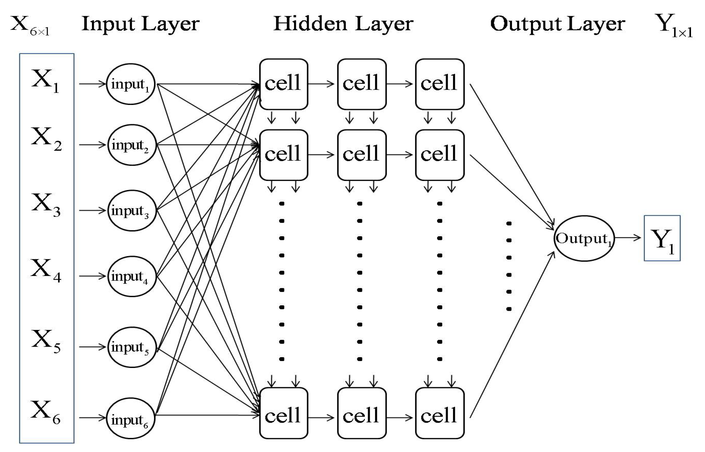
As for the selection of hyperparameters, we use different combinations of hyperparameters for experimental comparison. We select the hyperparameter combination with the lowest error metrics mean absolute percentage error (MAPE%) in

Table 1. The results of hyperparameters selection experimentation.

RNN-Unit	Input Size	Learning Rate	RNN-Hid Layer	Batch Size	Keep-Prob	MAPE%
40	6	0.0006	3	96	1	0.516494
60	7	0.001	4	120	1	0.928832
40	7	0.0001	4	48	0.9	1.87681
80	5	0.001	3	96	1	1.065048
60	4	0.0006	5	96	1	0.586579

. The input data includes the historical load data of the recent four time points, the sampling point and the temperature data of current time point (if the system determines that temperature should not be taken into account, the input value is 5). The parameter keep-prob works to make the neurons working with a certain probability during training. The LSTM neural network structure employed in this paper is illustrated in Figure 3. Here, the number of all hidden layer cells is equal. The LSTM model consists of one input layer, three hidden layers, and one output layer.

3.3. TFW

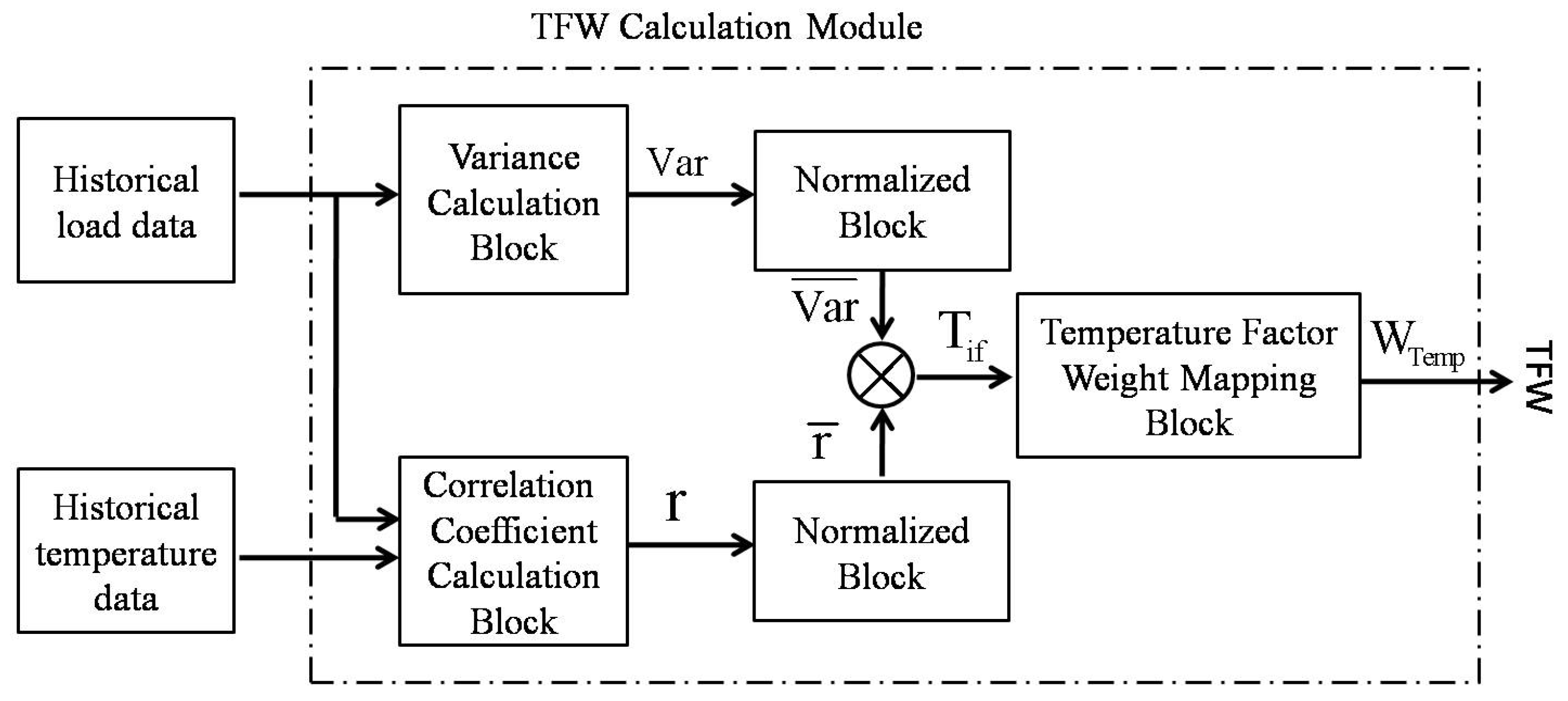
In this paper, a TFW calculation module is proposed to reflect the degree to which it is worth considering temperature in the process of predicting the current power load. The structure diagram of the TFW calculation module is presented in Figure 4. The algorithm flow is shown in Algorithm 1. The module inputs historical temperature data and historical load data. Subsequently, the model outputs the TFW value $W_{temp}$ through the intermediate variable temperature influence coefficient (TIC) $T_{if}$ and the mapping relation $f:T_{if}\to W_{temp}$. The module calculates the variance of the load value at the same time point across all dates in the historical data, while the sum of the corresponding variance of the 96 time points is represented by Var. Here, Var is used to reflect the degree of load fluctuation in the training data. As load fluctuation is mainly derived from weather-sensitive load, this variable can reflect the degree to which abrupt changes in weather-sensitive load are present in the training data. Variance calculation block is used to calculate the Var.

Algorithm 1 TFW Calculation Module.

Input:

Historical load data L;

Historical temperature data T;

Output:

TFW $W_{Temp}$;

1: Initialize: x = 1. 2: for each $j\in [1,96]$ do 3:   Calculate the variance of a sequence of historical data consisting of the jth point of the day; 4:   The calculated results are temporarily stored in x; 5:   sum = sum + x 6: end for 7: Var = sum/96 8: Calculate the covariance $Cov$ between L and T; 9: Calculate the correlation coefficient r between L and T; 10: Standardize r and Var; 11: Calculate Temperature Influence Coefficient $T_{if}$; 12: Calculate the TFW according to the mapping relation; 13: return$W_{temp}$;

Moreover, Var is calculated as Equation (4):

$$Var={\displaystyle \sum _{i=1}^{96}}\frac{{\sum }_{j=1}^N{(L_{ij}-\frac{1}{N}{\sum }_{j=1}^N{L}_{ij})}^2}{N}$$

(4)

Here, N represents the total number of days of historical data used, while $L_{ij}$ represents the load value. The formulas used to calculate the covariance and correlation coefficients are shown in Equations (5) and (6):

$$COV(X,Y)=E\left[\right(X-E\left(X\right)\left)\right(Y-E\left(Y\right)\left)\right]$$

(5)

$$R(X,Y)=\frac{COV(X,Y)}{\sqrt{var\left(X\right)var\left(Y\right)}}$$

(6)

Here, COV represents the covariance, while X and Y denote the temperature and power load, respectively. The normalized module is used to normalize the data. $T_{if}$ is calculated according to Equation (7):

$$T_{if}=\overline{R}·\overline{Var}$$

(7)

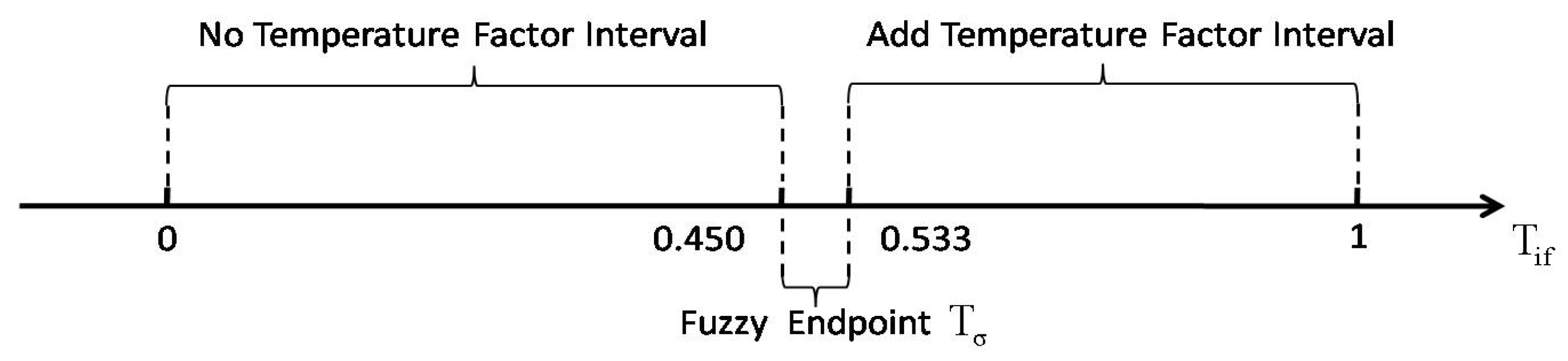
The TFW mapping block maps the corresponding interval according to the calculated TIC value $T_{if}$. As shown in Figure 5, the add temperature factor interval indicates that the TFW $W_{temp}$ is 100%, which indicates that the temperature must be considered in the calculation; moreover, the no temperature factor interval indicates that $W_{temp}$ is 0, which indicates that the temperature should not be considered. However, the fuzzy endpoint $T_{\sigma }$ is a critical value and is characterized by volatility, which is in turn caused by the randomness and volatility of the power load and temperature. In this paper, the floating ranges of the fuzzy endpoints $T_{\sigma }$ are obtained via experimental study.

Here, the TIC $T_{if}$ is located in the probability interval of the fuzzy endpoint $T_{\sigma }$ (0.450, 0.533), while $W_{Temp}$ is calculated according to Equation (8).

$$W_{temp}=\frac{T_{if}-0.45}{0.083}\times 100\%$$

(8)

Finally, the mapping relation $f:T_{if}\to W_{temp}$ between the TIC and the TFW is as presented in

Table 2. Mapping relation table.

Interval	TFW
Add Temperature Factor Interval	100%
NO Temperature Factor Interval	0%
Fuzzy Endpoint $T_{\sigma }$	$12.048·(T_{if}-0.45)\times 100\%$

.

3.4. Implementation of TFW-LSTM Method

3.4.1. Structure of TFW-LSTM Method

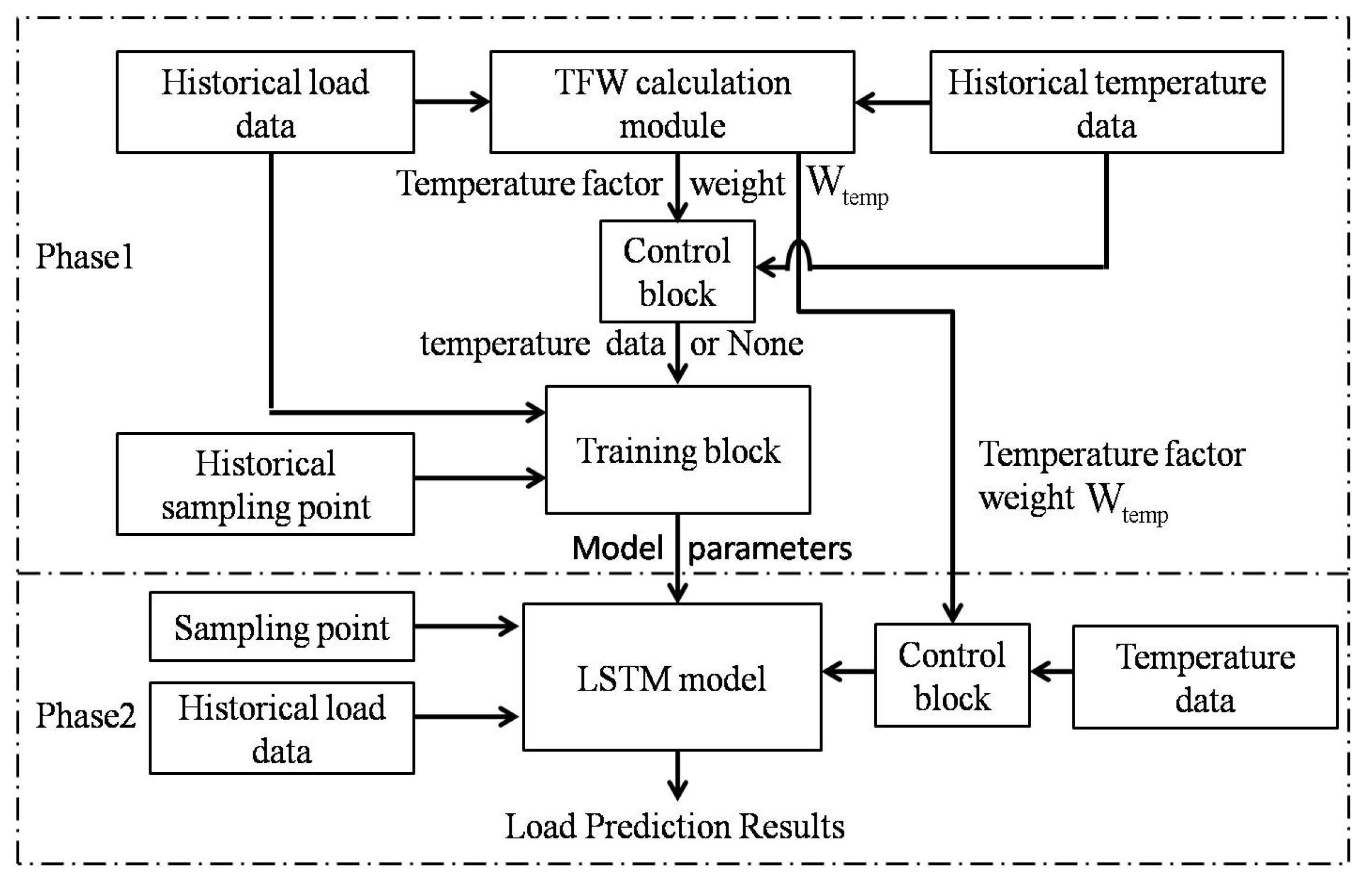
The present paper proposes a short-term power load forecasting method based on TFW and the LSTM model. The block diagram of the method is illustrated in Figure 6. In phase 1, the historical load data and historical temperature data are input into the TFW calculation module, after which the corresponding $W_{Temp}$ is calculated and output to the control block. Here, control block is a logical unit block that controls whether or not historical temperature data will be input into the neural network training module. When the TFW meets $W_{temp}\ge 50\%$, the control block decides that the temperature factor should be considered in the current prediction work, with the result that the historical temperature data will be passed through the control block; otherwise, historical temperature data are not allowed to pass, and the output value is None. In the next step, the training block receives the historical load data and the historical sampling point data simultaneously. The AdamOptimizer, under the tensorflow framework, is used for training so that the optimal parameters of the model can be found. Once the training is completed, the optimal parameters of the output model are sent on to the LSTM model for testing.

The control block of phase 2 receives the $W_{Temp}$ calculated in phase 1 to control the temperature data used in the current forecast. The LSTM model receives the sampling point, the return value of control block and the optimal model parameters as input, then outputs the corresponding power load prediction results.

3.4.2. Experimental Configuration

In this paper, 39 dates are randomly selected in 2019 as testing set. The data of 10 days’ prior to each experimental prediction date are used for training. Therefore, the ratio of the training set to the test set is 10:1. During the experiments, the trained model is used to output the predicted load value corresponding to the predicted time point. Furthermore, the model output value is compared with the label value to calculate the error. Finally, four test sets are extracted to facilitate comparison between the proposed method and the traditional power load forecasting methods. Due to the large number of missing data points, the data for February are not used in this paper.

This article employs three performance metrics to evaluate the results of the model testing: MAPE, mean absolute error (MAE), and root mean square error (RMSE).

The $MAPE$ is defined as follows.

$$MAPE=\frac{1}{n}{\displaystyle \sum _{i=1}^n}\left|\frac{\widetilde{y_i}-y_i}{y_i}\right|\times 100\%$$

(9)

The $MAE$ is defined as follows.

$$MAE=\frac{1}{n}{\displaystyle \sum _{i=1}^n}\left|\widetilde{y_i}-y_i\right|$$

(10)

The $RMSE$ is defined as follows.

$$RMSE=\sqrt{\frac{1}{n}{\displaystyle \sum _{i=1}^n}{\left(\widetilde{y_i}-y_i\right)}^2}$$

(11)

Here, the $\tilde{y}$ denotes the result of the model, while $\tilde{y}$ represents the true value and n is the total number of calculated values.

4. Results and Discussion

In order to verify the performance of the TFW-LSTM method, data from a certain region in Hunan, China in 2019 were selected for comparative experiments. Among them, 39 dates were randomly selected to compare the performance of the proposed method with the traditional LSTM, and the TIC $T_{if}$ in each dates was calculated simultaneously. The experimental data results were shown in

Table 3. Experimental result from January to September.

$\mathbf{Prediction}\mathbf{Date}$	$\mathbf{Proposed}\mathbf{Method}$			$\mathbf{Traditional}\mathbf{LSTM}\mathbf{Model}$			${\mathit{T}}_{\mathit{if}}$
	MAPE%	MAE	RMSE	MAPE%	MAE	RMSE
12 January 2019	1.227	63.163	103.183	1.463	77.701	114.354	0.075
18 January 2019	1.153	56.607	85.589	1.630	83.032	127.219	0.102
24 January 2019	1.241	54.110	84.717	1.946	82.014	117.868	0.206
12 March 2019	1.246	43.658	65.677	1.357	47.994	74.596	0.162
17 March 2019	1.202	42.803	69.275	2.405	85.847	110.384	0.110
20 March 2019	0.790	27.635	38.617	1.981	63.316	84.662	0.039
28 March 2019	1.718	56.029	117.487	2.399	82.745	144.635	0.059
13 April 2019	1.525	49.922	71.111	1.968	65.622	93.890	0.099
20 April 2019	0.918	30.824	43.712	1.654	55.777	76.264	0.012
30 April 2019	1.096	35.621	50.803	1.619	52.045	73.962	0.046
4 May 2019	1.293	42.546	66.575	1.836	61.701	90.558	0.253
12 May 2019	1.118	36.729	54.485	1.597	51.431	70.312	0.126
23 May 2019	1.062	37.021	56.133	1.507	49.843	74.977	0.007
31 May 2019	1.192	39.722	61.448	1.821	57.460	74.052	0.137
12 June 2019	1.451	57.441	78.488	1.526	60.385	82.375	0.578
20 June 2019	1.119	55.520	87.815	1.572	80.519	119.348	0.284
30 June 2019	1.390	56.590	88.353	1.458	58.247	85.244	0.904
13 July 2019	1.564	57.286	80.040	1.583	60.550	94.416	0.637
20 July 2019	1.421	78.423	110.185	1.345	74.223	107.056	0.980
27 July 2019	1.025	66.570	97.223	0.957	61.890	88.563	0.594
31 July 2019	0.502	32.783	42.402	1.159	68.649	86.243	0.533
6 August 2019	0.638	42.122	61.446	0.766	48.252	65.227	0.209
10 August 2019	0.604	36.360	52.501	0.836	49.441	65.596	0.236
20 August 2019	0.726	46.776	66.012	0.882	55.004	75.880	0.281
31 August 2019	1.150	51.518	67.147	1.194	77.397	94.842	0.699
8 September 2019	1.059	55.734	89.783	1.145	61.295	92.147	0.540
24 September 2019	1.313	52.112	78.539	1.510	56.266	85.089	0.450
28 September 2019	1.117	42.166	59.831	1.257	51.505	75.338	0.048
3 October 2019	1.247	46.173	65.438	2.061	69.810	88.587	0.196
13 October 2019	1.215	43.057	66.225	1.926	66.577	89.706	0.336
19 October 2019	1.106	39.967	59.553	1.218	43.722	62.159	0.026
30 October 2019	1.120	40.293	67.258	1.377	47.215	62.717	0.010
7 November 2019	0.651	23.465	29.651	1.205	44.648	69.212	0.038
14 November 2019	0.919	33.960	56.952	1.145	43.583	67.244	0.000
20 November 2019	1.158	43.012	67.328	1.359	52.550	85.253	0.043
30 November 2019	1.918	87.432	117.466	3.755	184.180	244.727	0.000
8 December 2019	0.908	39.555	63.833	1.631	72.002	106.587	0.120
24 December 2019	0.797	38.797	50.369	3.375	156.705	201.106	0.088
31 December 2019	1.402	72.795	106.010	1.636	80.844	112.853	0.093

.

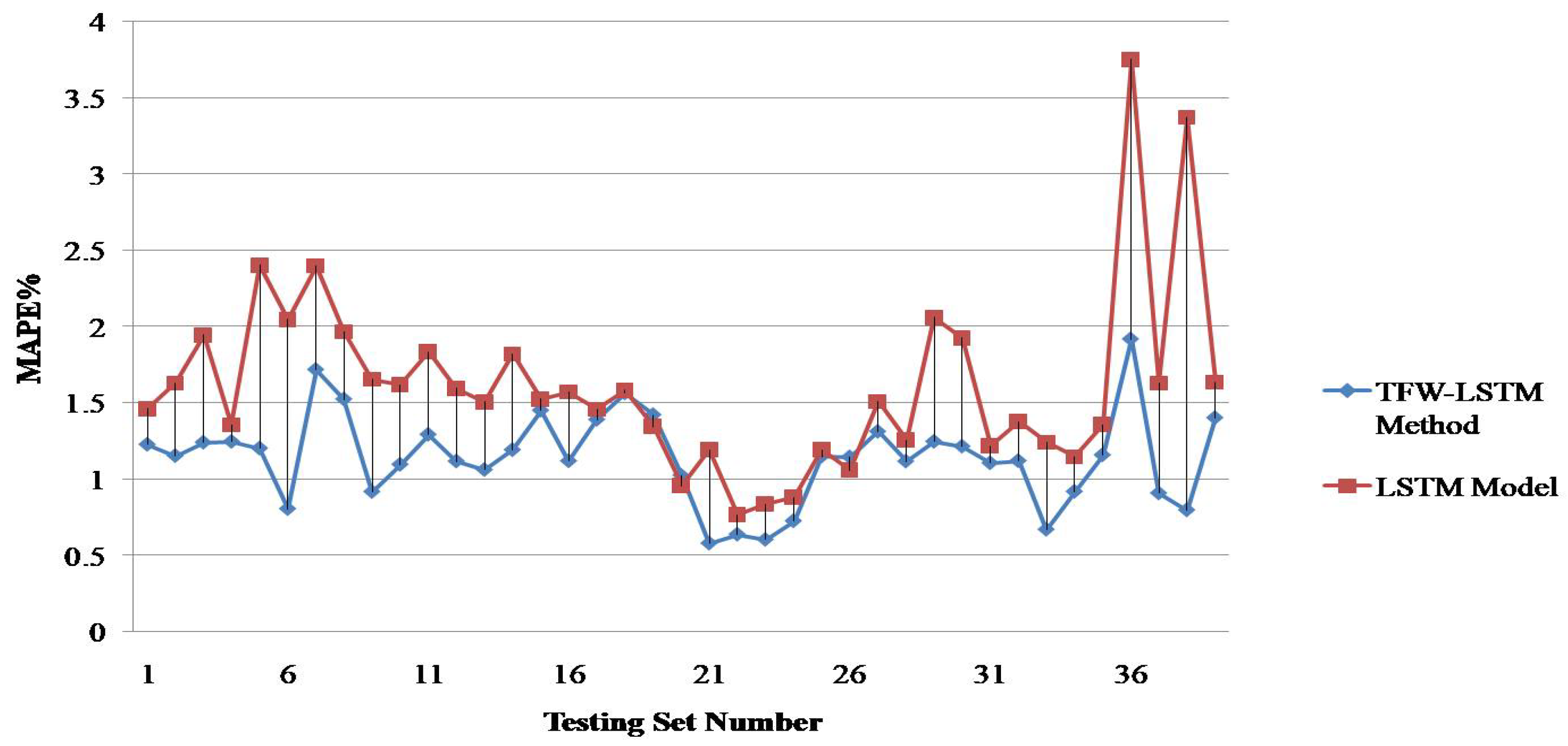
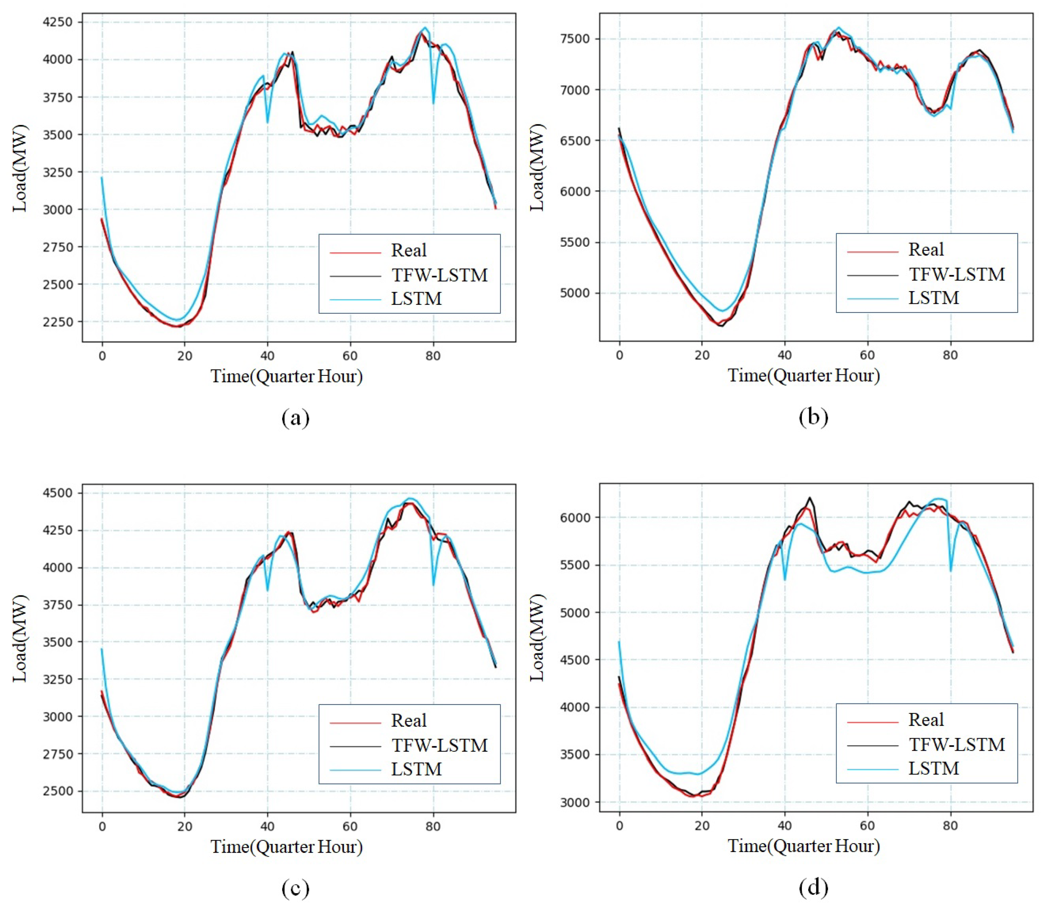
The experiments were conducted on a laptop with Intel(R) Core(TM) i7-8750H CPU 2.20 GHZ, 64-bit Windows 10 operating system and 8GB memory, using Python 3.7.4 in the tensorflow framework. The MAPE% comparison between the TFW-LSTM method and traditional LSTM model were presented in Figure 7, and we also selected 4 typical days for further study. The results of comparison was illustrated in Figure 8.

It can be concluded from the experimental results that the proposed method performs better overall and was generally more stable than the traditional LSTM model. Moreover, because the TFW-LSTM method was able to flexibly apply the temperature factor in the power load forecasting process, it was better able to absorb the advantages of utilizing the temperature factor while avoiding the associated disadvantages.

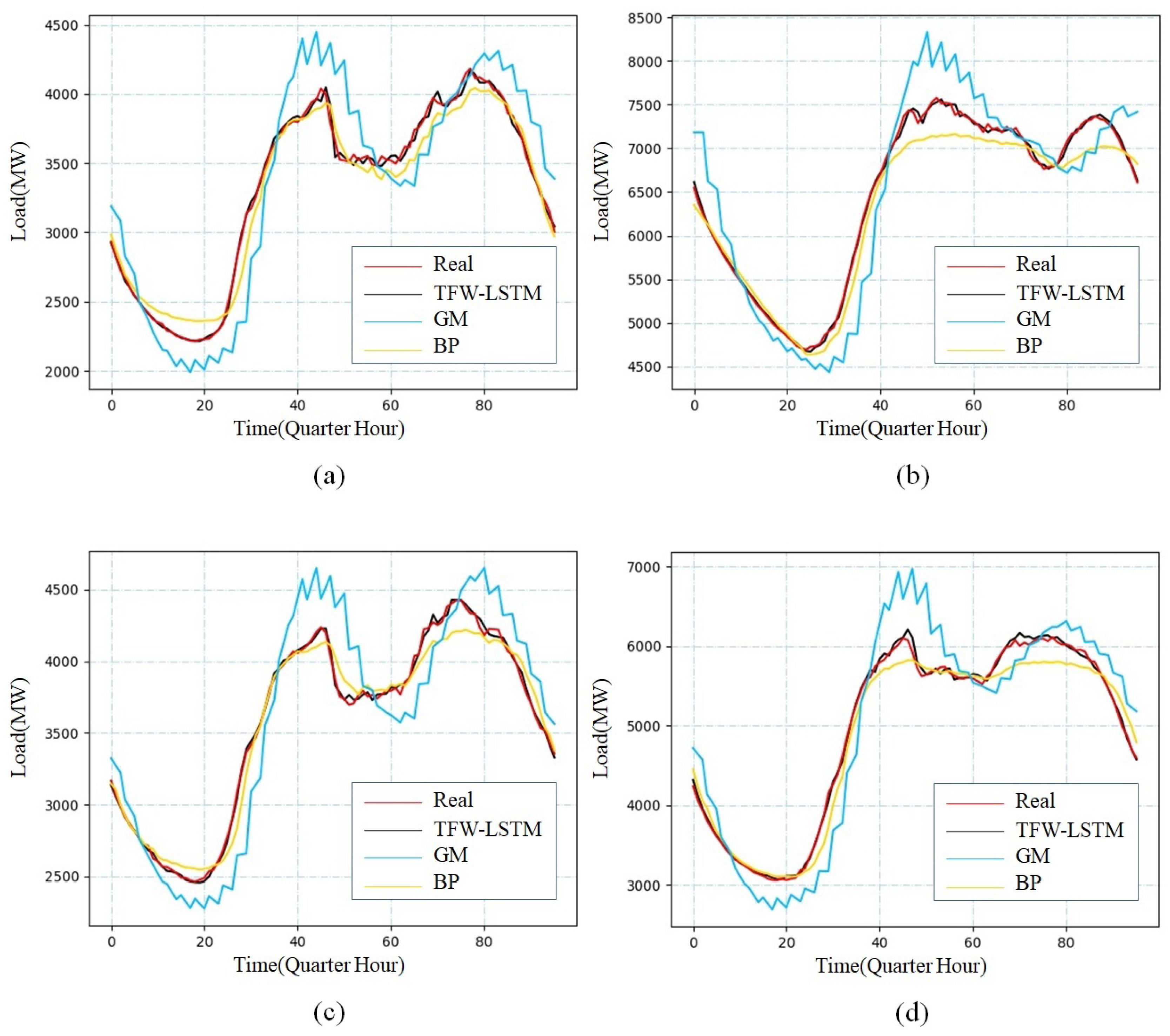
In the next step, so as to more objectively demonstrate the superiority of the proposed method, the proposed method was compared with the BP neural network and traditional grey model in the four typical dates above. The results of metric were listed in

Table 4. The comparison result table of proposed method and traditional method.

$\mathbf{Date}$	$\mathbf{TFW}-\mathbf{LSTM}\mathbf{Method}$			$\mathbf{BP}\mathbf{Neural}\mathbf{Network}$			$\mathbf{Grey}\mathbf{Model}$
	MAPE%	MAE	RMSE	MAPE%	MAE	RMSE	MAPE%	MAE	RMSE
20 March	0.79	27.63	38.61	2.85	89.11	106.56	7.76	252.16	302.10
31 July	0.50	32.78	42.40	2.47	165.66	200.96	5.32	341.48	427.58
7 November	0.65	23.46	29.65	2.04	73.38	96.71	6.80	241.92	286.86
24 December	0.79	39.69	53.18	2.87	144.66	176.36	7.70	362.18	442.44

, and the line graph was presented in Figure 9.

As we can see in the results, the TFW-LSTM method was obviously superior to other traditional methods in each metrics. In the four typical dates, the proposed method reduced MAPE by 1.24%, 1.68% and 6.21% on average, respectively, compared with the traditional LSTM, BP, and GM. Compared with LSTM, the TFW-LSTM method added the dynamic controlling mechanism of feature, and can show higher stability and prediction accuracy in USTLF. In contrast with other traditional prediction methods, the TFW-LSTM method had a great advantage because of its inherent nonlinear processing ability and temporal data processing ability.

5. Conclusions

In order to eliminate the negative influence of temperature on load prediction in USTLF, we propose a method for USTLF based on TFW and the LSTM model. The TFW calculation module is the core of the proposed method, which determines whether the temperature factor should be considered.

The proposed method is based on TFW and the LSTM model, which uses real data from a region in Hunan Province, China in 2019 for performance verification. The results show that compared with the traditional load forecasting method, the proposed method evaluates the importance of temperature to forecasting at the current time. It dynamically avoids the negative impact of temperature, and achieves a higher prediction accuracy by combining with the LSTM model. The performance metrics MAPE, MAE, and RMSE reflect the superiority of the proposed method.

In the future, as deep learning theory comes to be utilized more widely in data processing [32,33,34], we will attempt to use additional methods to improve both the accuracy of power load prediction and the overall model stability. In recent years, with the development of nonlinear system theory and research [35,36], we will try to adopt nonlinear time series forecasting models based on chaos theory for power load forecasting. We will also consider adopting image data processing methods [37,38] for power load forecasting.

References

- Hong, T.; Fan, S. Probabilistic electric load forecasting:a tutorial review. Int. J. Forecast. 2016, 32, 914–938. [Google Scholar] [CrossRef]
- Wang, Q.; Zhang, C.; Ding, Y.; Xydis, G.; Wang, J.; Østergaard, J. Review of real-time electricity markets for integrating distributed energy resources and demand response. Appl. Energy 2015, 138, 695–706. [Google Scholar] [CrossRef]
- Jia, Z.; Fan, Z.; Li, C.; Jiang, M. The Application of Improved Grey GM(1,1) Model in Power System Load Forecast. Future Wirel. Netw. Inf. Syst. 2011, 144, 603–608. [Google Scholar]
- Song, J.; Shu, H.; Dong, J.; Liang, Y.; Li, Y.; Yang, B. Comprehensive Load Forecast Based on GM(1,1) and BP Neural Network. Electr. Power Constr. 2020, 41, 75–80. [Google Scholar] [CrossRef]
- Liu, C.-W.; Zhao, H.-K.; Yan, H.; Wang, J.-H. Power Load Forecasting Based on Fractional GM(1,1) and BP Neural Network. Math. Pract. Theory 2018, 48, 145–151. [Google Scholar]
- Long, Y.; Su, Z.; Wang, Y. Monthly load forecasting model based on seasonal adjustment and BP neural network. Syst. Eng. Theory Pract. 2018, 38, 1052–1060. [Google Scholar] [CrossRef]
- Ge, Q.; Jiang, H.; He, M.; Zhu, Y.; Zhang, J. Power Load Forecast Based on Fuzzy BP Neural Networks with Dynamical Estimation of Weights. Int. J. Fuzzy Syst. 2020, 22, 956–969. [Google Scholar] [CrossRef]
- Hu, Y.-C. Electricity consumption prediction using a neural network based grey forecasting approach. J. Oper. Res. Soc. 2017, 68, 1259–1264. [Google Scholar] [CrossRef]
- Rim, H.; Mourad, Z.; Ousama, B.-S. Short-term electric load forecasting in Tunisia using artificial neural networks. Energy Syst. 2020, 11, 357–375. [Google Scholar] [CrossRef]
- Behm, C.; Nolting, L.; Praktiknjo, A. How to Model European Electricity Load Profiles using Artificial Neural Networks. Appl. Energy 2020, 277, 115564. [Google Scholar] [CrossRef]
- Pal, S.S.; Kar, S. A hybridized forecasting method based on weight adjustment of neural network using generalized type-2 fuzzy set. Int. J. Fuzzy Syst. 2019, 21, 308–320. [Google Scholar] [CrossRef]
- Imtiaz, P.; Arif, S.; Anjan, D.; Temitayo, O.; Md Golam, D. Multi-Layer Perceptron Based Photovoltaic Forecasting for Rooftop PV Applications in Smart Grid. 2020. Available online: https://www.researchgate.net/publication/338852633 (accessed on 26 August 2020).
- Tong, Y.; Liu, Y.; Wang, J.; Xin, G. Text Steganography on RNN-Generated Lyrics. Math. Biosci. Eng. 2019, 16, 5451–5463. [Google Scholar] [CrossRef]
- Xiang, L.; Yang, S.; Liu, Y.; Li, Q.; Zhu, C. Novel Linguistic Steganography Based on Character-Level Text Generation. Mathematics. 2020, 8, 1558. Available online: https://0-doi-org.brum.beds.ac.uk/10.3390/math8091558 (accessed on 17 September 2020). [CrossRef]
- Wang, J.; Qin, J.; Xiang, X.; Tan, Y.; Pan, N. CAPTCHA recognition based on deep convolutional neural network. Math. Biosci. Eng. 2019, 16, 5851–5861. [Google Scholar] [CrossRef]
- Zhang, Y.; Lu, W.; Ou, W.; Zhang, G.; Zhang, X.; Cheng, J.; Zhang, W. Chinese medical question answer selection via hybrid models based on CNN and GRU. Multimed. Tools Appl. 2020, 79, 14751–14776. [Google Scholar] [CrossRef]
- Luo, Y.; Qin, J.; Xiang, X.; Tan, Y.; Liu, Q.; Xiang, L. Coverless real-time image information hiding based on image block matching and Dense Convolutional Network. J. Real-Time Image Proc. 2020, 17, 125–135. [Google Scholar] [CrossRef]
- Hochreiter, S.; Schmidhuber, J. Long short-term memory. Neural Comput. 1997, 9, 1735–1780. [Google Scholar] [CrossRef]
- Muzaffar, S.; Afshari, A. Short-Term Load Forecasts Using LSTM Networks. Energy Procedia 2019, 158, 2922–2927. [Google Scholar] [CrossRef]
- Santra, A.S.; Lin, J.-L. Integrating Long Short-Term Memory and Genetic Algorithm for Short-Term Load Forecasting. Energies 2019, 12, 2040. [Google Scholar] [CrossRef] [Green Version]
- Qing, X.; Niu, Y. Hourly day-ahead solar irradiance prediction using weather forecasts by LSTM. Energy 2018, 148, 461–468. [Google Scholar] [CrossRef]
- Li, S. LSTM Recurrent Neural Network Short-Term Power Load Forecasting Based on TensorFlow. Shanghai Energy Conserv. 2018, 7, 974–977. [Google Scholar]
- Chen, Z.; Liu, J.; Li, C.; Ji, X.; Li, D.; Huang, Y.; Di, F. Ultra Short-term Power Load Forecasting Based on Combined LSTM-XGBoost Model. Power System Technol. 2019, 44, 614–620. [Google Scholar] [CrossRef]
- Zhang, M.; Du, Y.; Hong, G. Application of LSTM in Yichang Short-term Power Load Forecasting. J. Meteorol. Res. Appl. 2019, 40, 72–77. [Google Scholar] [CrossRef]
- Liu, P.; Zheng, P.; Chen, Z. Deep Learning with Stacked Denoising Auto-Encoder for Short-Term Electric Load Forecasting. Energies 2019, 12, 2445. [Google Scholar] [CrossRef] [Green Version]
- Kulkarni, S.; Simon, S.P. A spiking neural network (SNN) forecast engine for short-term electrical load forecasting. Appl. Soft Comput. 2013, 13, 28–35. [Google Scholar] [CrossRef]
- Wang, H.; Xue, W.; Liu, Y.; Peng, J.; Jiang, H. Probabilistic wind power forecasting based on spiking neural network. Energy 2020, 196. [Google Scholar] [CrossRef]
- Udaya, B.R.; Alberto, M.; Anton, S.; Henrik, J.; Calogero, M.O. Cuneate spiking neural network learning to classify naturalistic texture stimuli under varying sensing conditions. Neural Netw. 2020, 123, 273–287. [Google Scholar] [CrossRef]
- Zhang, N.; Li, Z.; Zou, X.; Quiring, S.M. Quiring. Comparison of three short-term load forecast models in Southern California. Energy 2019, 189, 1–11. [Google Scholar] [CrossRef]
- Li, B.; Men, D.; Yang, J.; Zhou, J. Bus load Forecasting Based on Numerical Weather Prediction. Autom. Electr. Power Syst. 2015, 39, 137–140. [Google Scholar] [CrossRef]
- Yuan, S.; Zhang, G.; Zhang, J. Integrated Forecasting Model of Bus Load Based on Numerical Weather Prediction. Power Syst. Autom. 2019, 41, 62–65. [Google Scholar] [CrossRef]
- Wang, J.; Gu, X.; Liu, W. An Empower Hamilton Loop based Data Collection Algorithm with MobileAgent for WSNs. Hum.-Cent. Comput. Inf. Sci. 2019, 9, 1–14. [Google Scholar] [CrossRef]
- Wang, J.; Yang, Y.; Wang, T. Big Data Service Architecture: A Survey. J. Internet Technol. 2020, 21, 393–405. [Google Scholar]
- Zhang, J.; Zhong, S.; Wang, T. Blockchain-Based Systems and Applications: A Survey. J. Internet Technol. 2020, 21, 1–14. [Google Scholar]
- Yu, F.; Liu, L.; Xiao, L.; Li, K.; Ca, S. A robust and fixed-time zeroing neural dynamics for computing time-variant nonlinear equation using a novel nonlinear activation function. Neurocomputing 2019, 350, 108–116. [Google Scholar] [CrossRef]
- Yu, F.; Liu, L.; He, B.; Huang, Y.; Shi, C.; Cai, S.; Song, Y.; Du, S.; Wan, Q. Analysis and FPGA Realization of a Novel 5D Hyperchaotic Four-Wing Memristive System, Active Control Synchronization, and Secure Communication Application. Complexity 2019, 1, 1–18. [Google Scholar] [CrossRef] [Green Version]
- Zhang, D.; Yang, G.; Li, F. Detecting seam carved images using uniform local binary patterns. Multimed. Tools Appl. 2018, 79, 8415–8430. [Google Scholar] [CrossRef]
- Ding, X.; Zhang, D. Detection of motion-compensated frame-rate up-conversion viaoptical flow-based prediction residue. Optik 2020, 207, 1637–1649. [Google Scholar] [CrossRef]
Figure 1.
Long short-term memory (LSTM) network structure.
Figure 2.
Structure diagram of LSTM cell.
Figure 3.
The structure of LSTM neural network.
Figure 4.
Structure of Temperature Factor Weight Calculation Module.
Figure 5.
Significance map of temperature influence coefficient.
Figure 6.
Block diagram of the proposed method.
Figure 7.
The mean absolute percentage error (MAPE%) comparison of TFW-LSTM method and traditional LSTM model.
Figure 8.
Prediction results for (a) 20 March 2019, (b) 31 July 2019, (c) 7 November 2019, and (d) 24 Decmber 2019. The “Real” stands for the actual value, and the TFW-LSTM is our method, the “LSTM” is the traditional LSTM model.
Figure 9.
Prediction results for (a) 20 March 2019, (b) 31 July 2019, (c) 7 November 2019, and (d) 24 Decmber 2019. The “Real” stands for the actual value, the TFW-LSTM is our method, the “GM” is the traditional gray model, and the “BP” is the traditional back propagation neural network model.