Comparison of Profitability of PV Electricity Sharing in Renewable Energy Communities in Selected European Countries


Abstract
:1. Introduction
1.1. Motivation
1.2. State of the Art
1.3. Progress Beyond the State of the Art
1.4. Outline
2. Materials and Methods
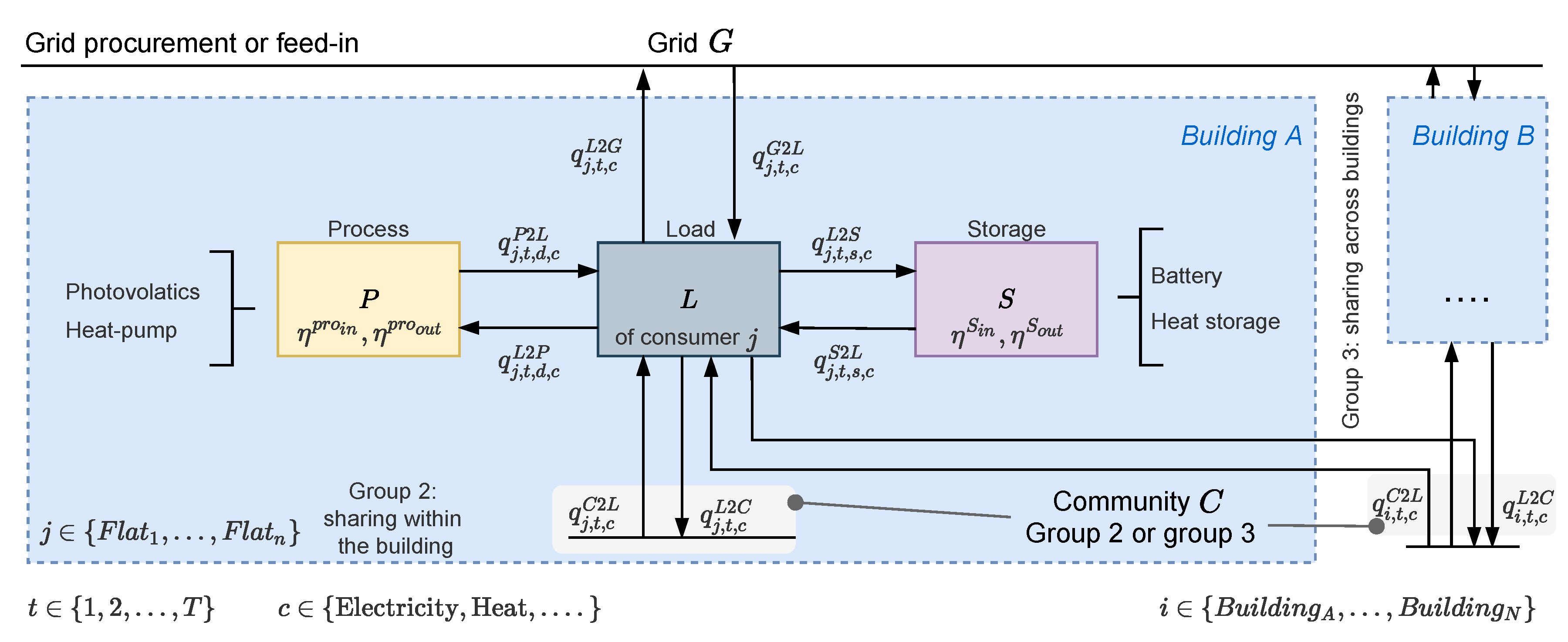
2.1. Optimization Problem and Nomenclature
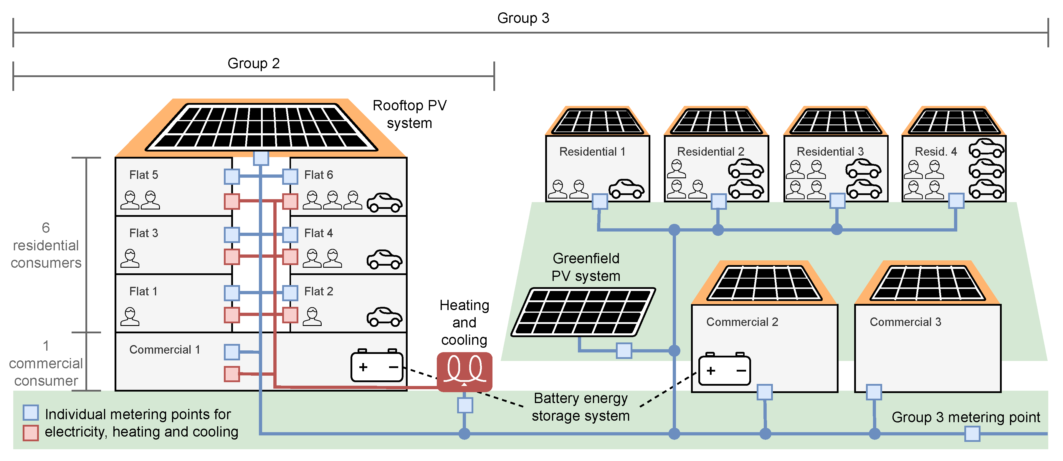
2.2. Definition of Scenarios
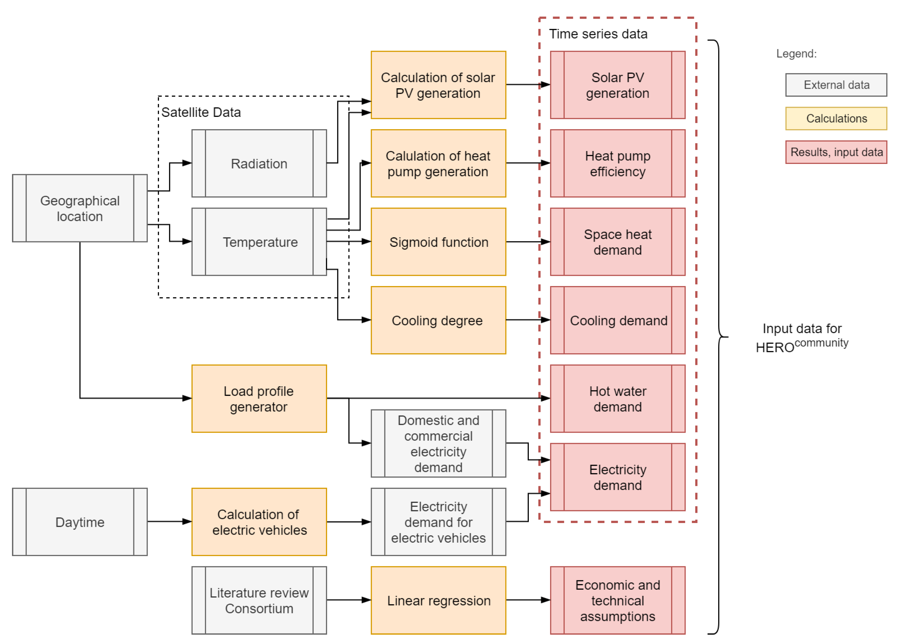
2.3. Input Data and Used Models
2.3.1. Electricity Demand Model
2.3.2. PV Generation Model
2.3.3. Heat Pump Efficiency Model
2.3.4. Heat and Hot Water Demand
2.3.5. Cooling Demand Model
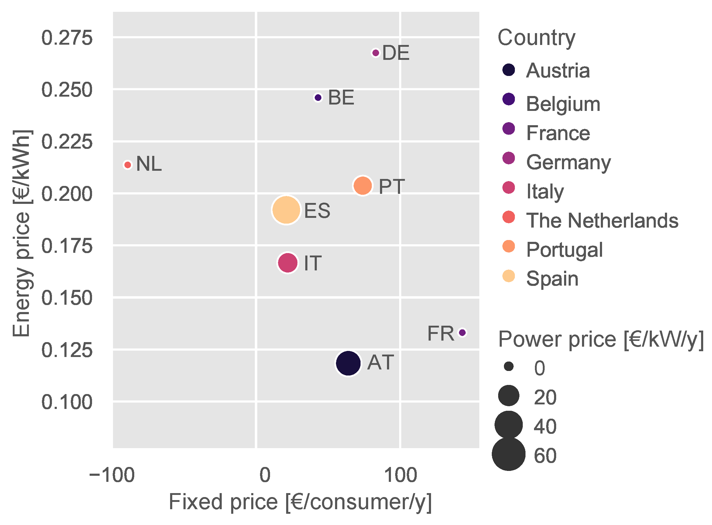
2.3.6. Electricity Procurement Prices and Feed-In Remuneration
- Energy component (€/kWh): The price for procured electric energy.
- Power component (€/kW/y): Price for maximum procured electric power, which is either the contracted or measured power per year.
- Fixed component (€/consumer/y): Annual fixed costs independent of electricity procurement.
2.3.7. Investment Costs
3. Results
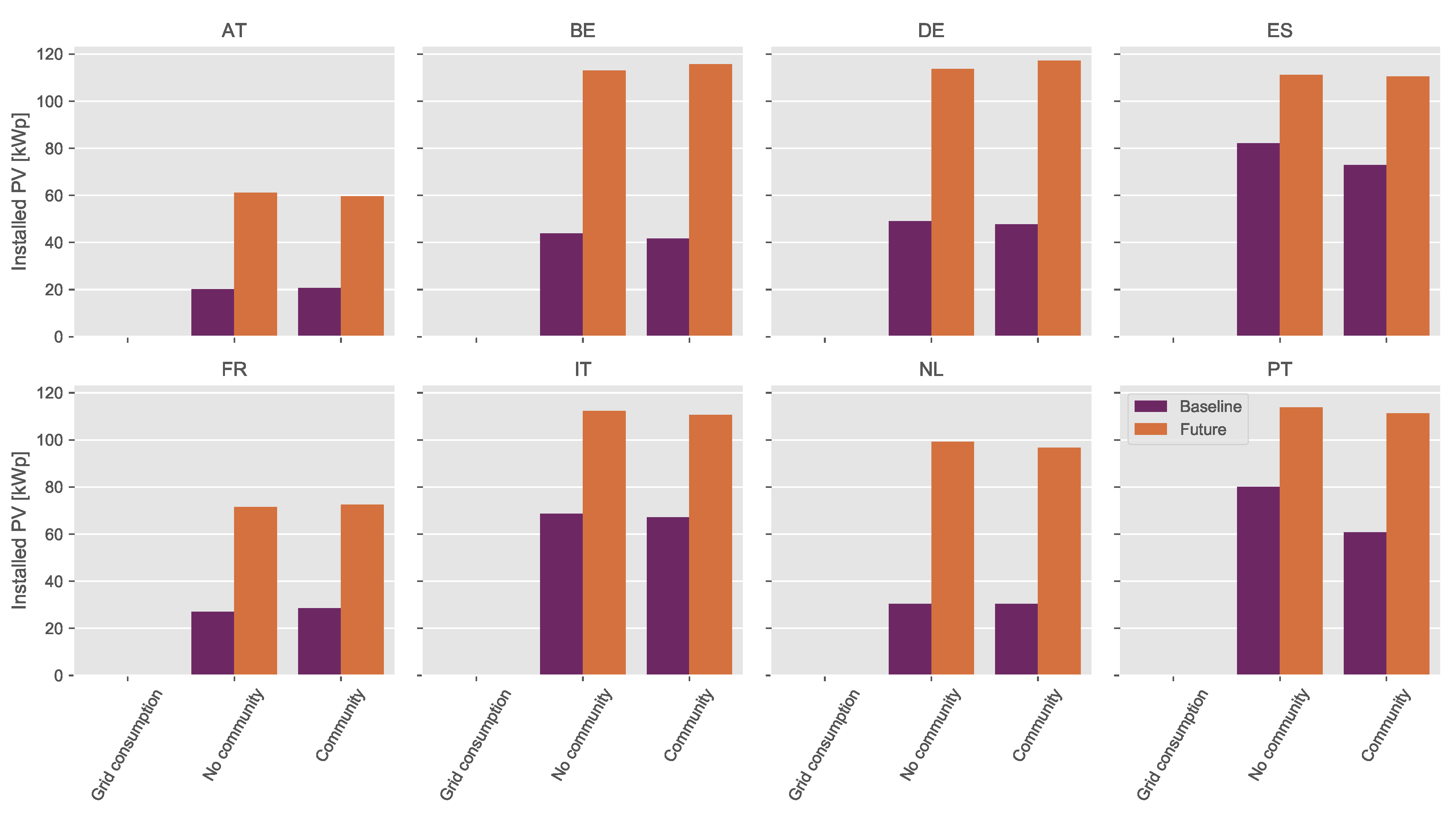
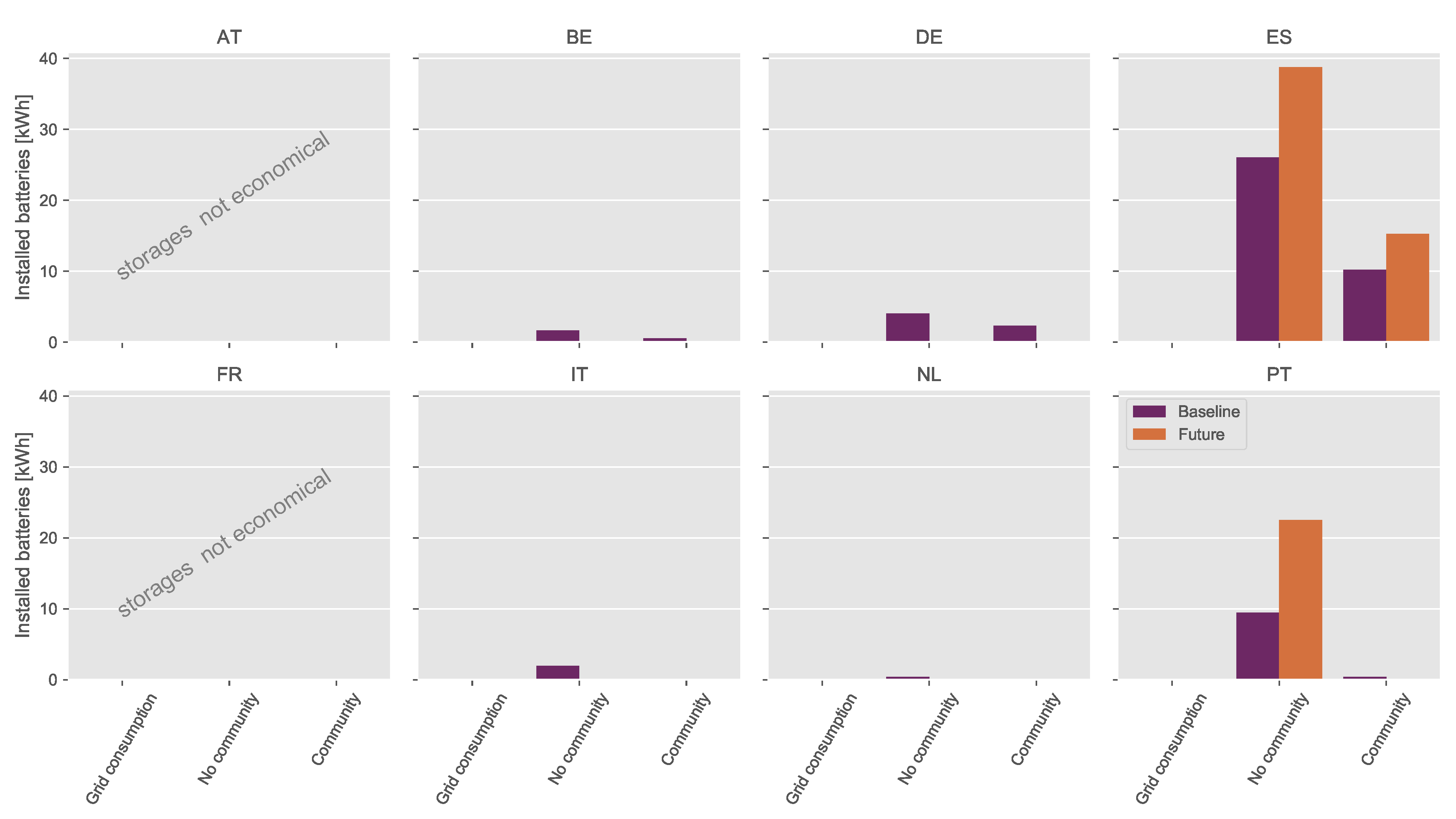
3.1. Investment Patterns
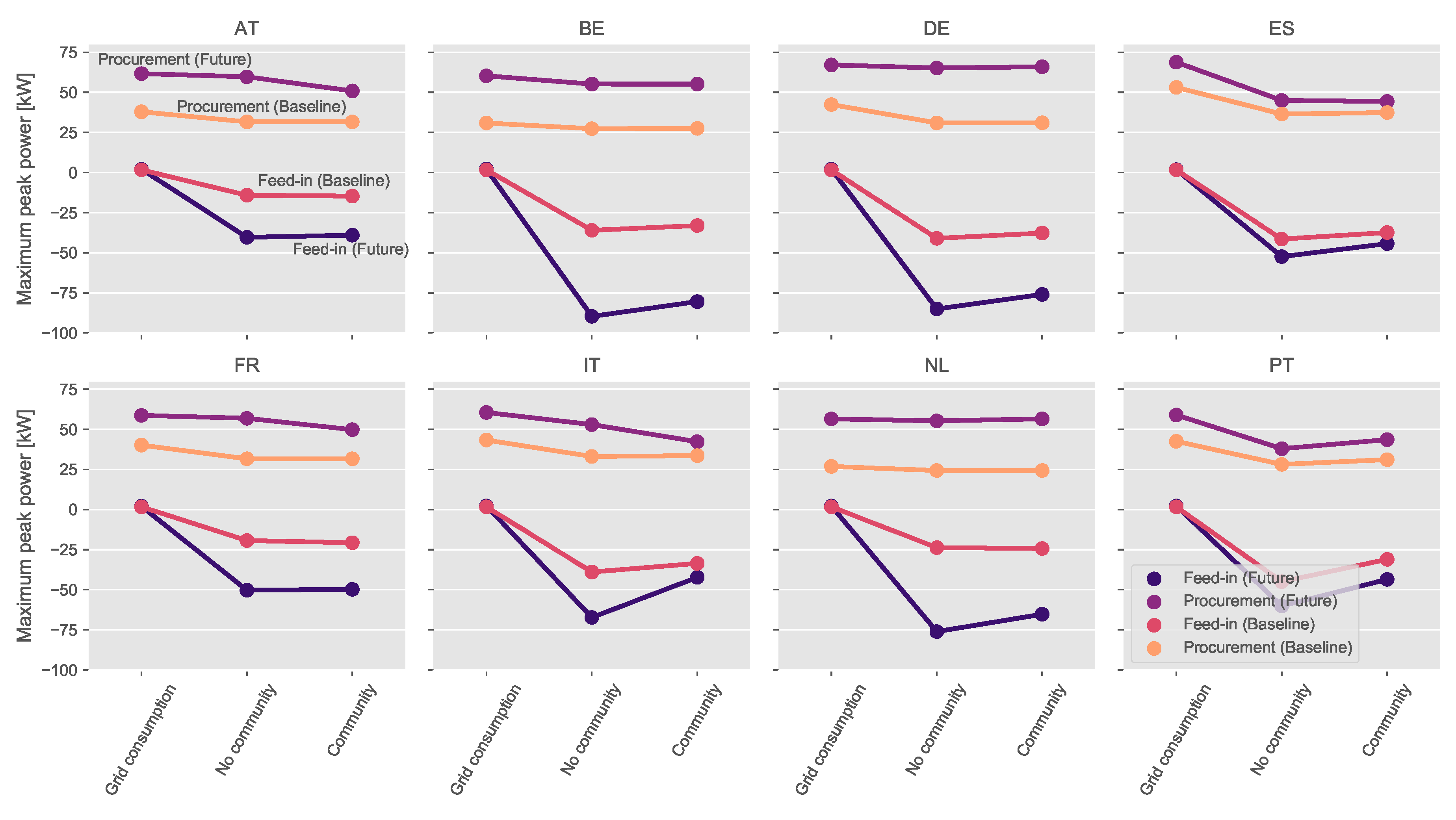
3.2. Peak Power
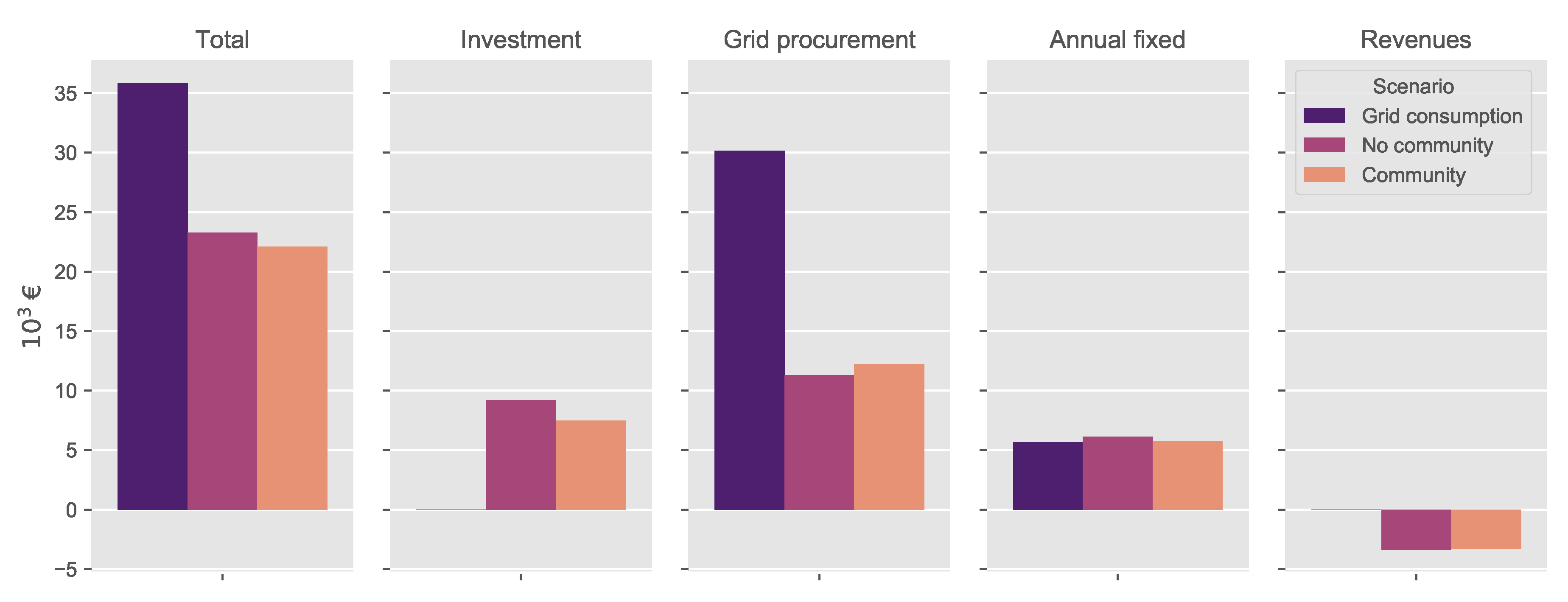
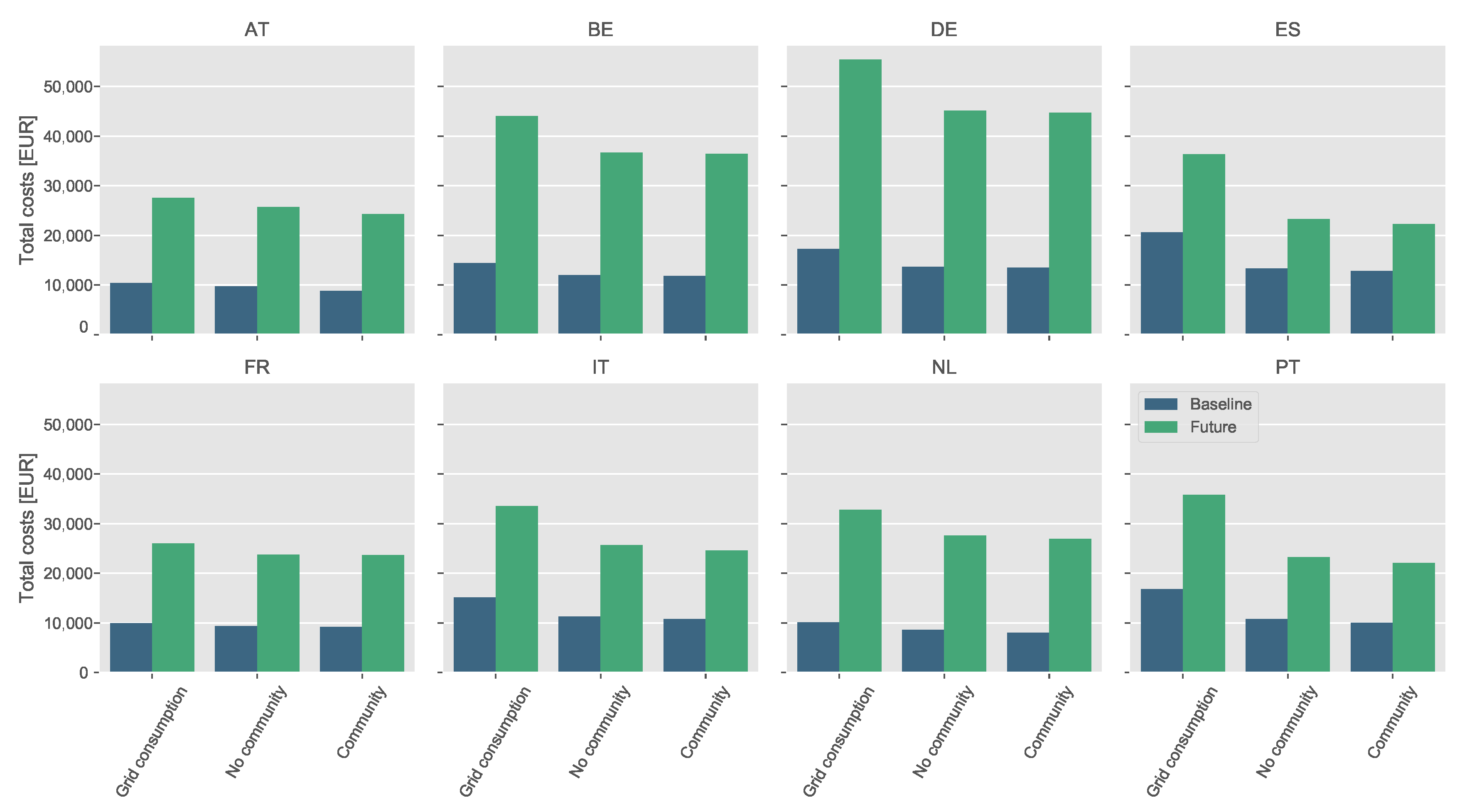
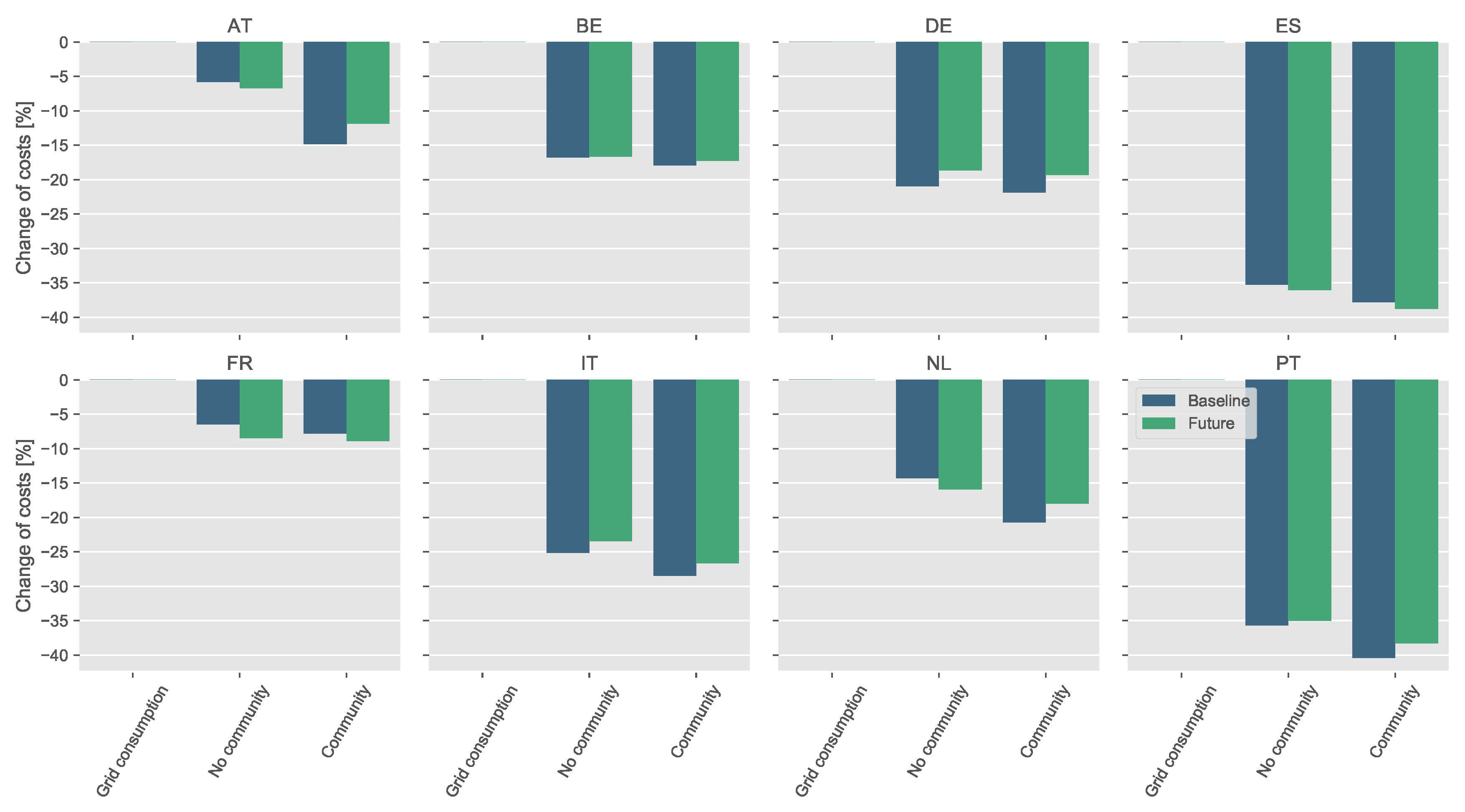
3.3. Costs
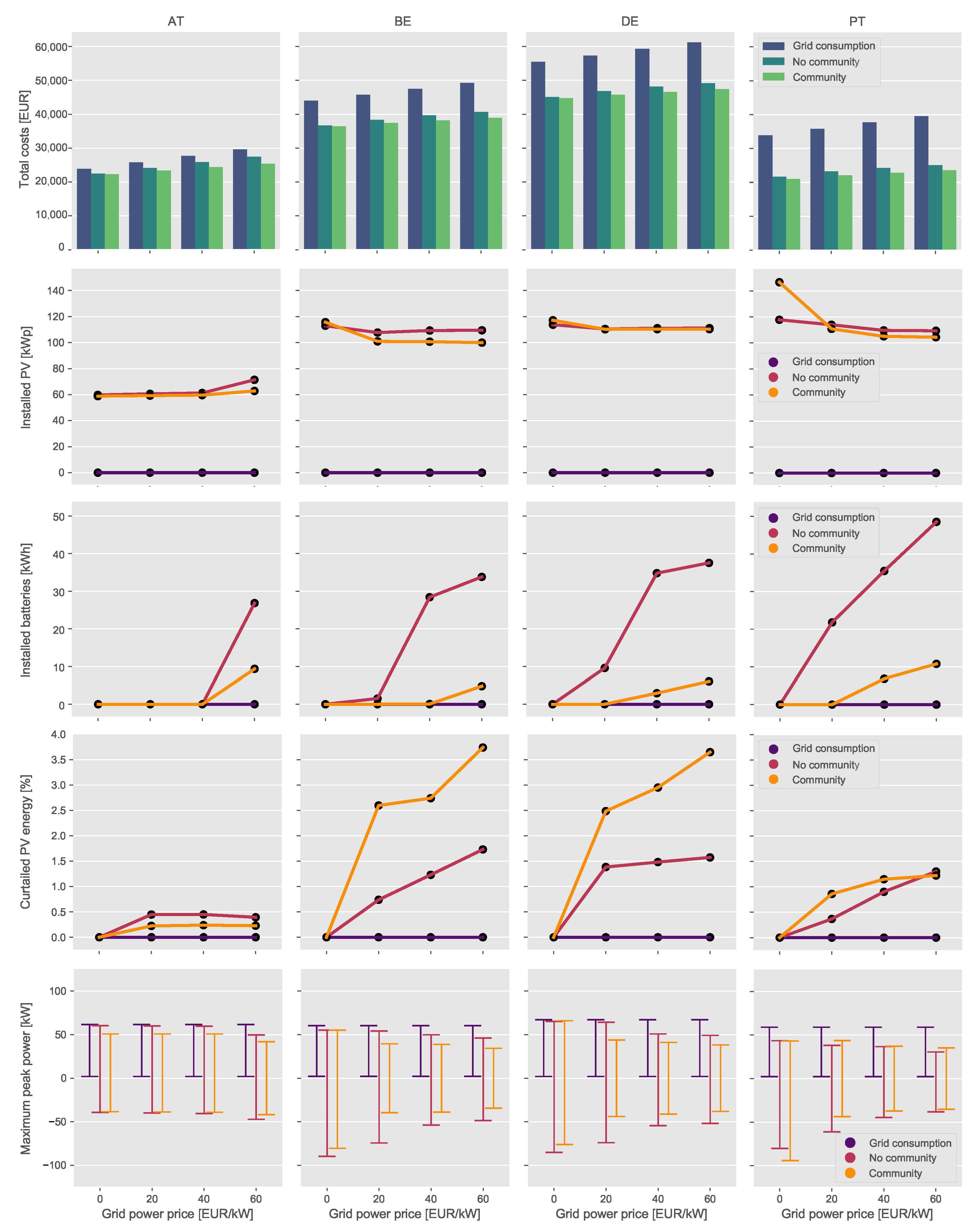
3.4. Sensitivity of Power Prices
3.5. Sensitivity of PV and BESS Prices
4. Discussion and Conclusions
Author Contributions
Funding
Acknowledgments
Conflicts of Interest
Abbreviations
| Nomenclature | |
| BESS | Battery Energy Storage Systems |
| CEC | Citizen Energy Community |
| DER | Distributed Energy Resources |
| DHW | Domestic Hot Water |
| EAC | Equivalent Annual Costs |
| EV | Electric Vehicle |
| P2P | Peer to Peer |
| LPG | Load Profile Generator |
| NPV | Net Present Value |
| PV | Photovoltaic |
| REC | Renewable Energy Community |
| RES | Renewable Energy Systems |
| SH | Space Heating |
| SOC | State-Of-Charge |
| TESS | Thermal Energy Storage Systems |
| Sets | |
| Time period | |
| Set of buildings | |
| Set of flats | |
| Set of energy commodities | |
| Set of storages | |
| Set of processes and DERs | |
| Variables | |
| Total costs per building for PV systems and BESS | |
| Total grid costs per building for power, fixed and energy component | |
| with | Energy flows from/to grid, load, storage, process or community |
| with | Maximum powers of flows from/to grid, load, storage, process or community |
| Binary variable for processes, and storages | |
| Maximum power for processes, and storages for commodity d per flat j | |
| Maximum storage capacity for commodity d per flat j | |
| Storage capacity at t | |
| Parameters | |
| Annual fixed prices for annuities of investments or other costs | |
| Annual power or capacity dependent prices for annuities of investments | |
| Input and output efficiencies for processes and storages | |
| Prices for procurement from the grid, -the community and feed-in remuneration | |
| r | interest rate |
| n | depreciation time |
Appendix A
Appendix A.1. Economic Assumptions

| Feed-In Remuneration | AT | BE | DE | ES | FR | IT | NL | PT |
|---|---|---|---|---|---|---|---|---|
| Average day-ahead price [€/MWh] | 34.19 | 44.58 | 34.19 | 52.24 | 44.97 | 51.61 | 39.31 | 52.48 |
| Exchanging Energy with | AT | BE | DE | ES | FR | IT | NL | PT |
|---|---|---|---|---|---|---|---|---|
| Group 2 [€/kWh] | - | - | - | - | - | - | - | - |
| Group 3 [€/kWh] | 0.048 | 0.098 | 0.094 | 0.071 | 0.053 | 0.059 | 0.071 | 0.071 |
| Outside [€/kWh] | 0.120 | 0.250 | 0.270 | 0.190 | 0.130 | 0.170 | 0.210 | 0.20 |
Appendix A.2. Supplementary Data to the Electricity Demand Model
| Consumer | People | Cars | El. Consumption (baseline) [kWh/yr] | Electricity Profile |
|---|---|---|---|---|
| Flat1 | 1 | 0 | 1245 | LPG |
| Flat2 | 1 | 1 | 1402 | LPG |
| Flat3 | 1 | 0 | 1179 | LPG |
| Flat4 | 2 | 1 | 2264 | LPG |
| Flat5 | 2 | 0 | 2158 | LPG |
| Flat6 | 3 | 1 | 3191 | LPG |
| Commercial1 | - | - | 5719 | G0 |
| Residential1 | 2 | 1 | 2372 | LPG |
| Residential2 | 3 | 2 | 3226 | LPG |
| Residential3 | 4 | 2 | 2968 | LPG |
| Residential4 | 4 | 3 | 3464 | LPG |
| Commercial2 | - | - | 12030 | G1 |
| Commercial3 | - | - | 5719 | G4 |
- Energy consumption of 20 kWh for a distance of 100 km (based on Nissan Leaf ZE1, energy capacity of 62 kWh for max. 385 km, [72])
- Employed residents charge EVs 50% at commercials (work) and 50% when they are back at home
- Non-employed residents charge EVs 50% at commercials and 50% at home
- On weekends, less consumption than during weekdays, but charged also during the day
- Charging always with 3.6 kW (e.g., 16 A single phase, 230 V).
| Country | Passenger Car Density [48] | Traveled Distance [73] | Modeled Average Charging Demand |
|---|---|---|---|
| [Cars/1000 people] | [km/car/yr] | [kWh/car/day] | |
| AT | 555 | 14,311 | 8.8 |
| BE | 503 | 12,997 | 6.8 |
| DE | 555 | 14,107 | 8.6 |
| ES | 492 | 12,535 | 6.8 |
| FR | 479 | 12,997 | 6.8 |
| IT | 625 | 9596 | 6.6 |
| NL | 481 | 14,107 | 6.8 |
| PT | 470 | 12,535 | 6.8 |
Appendix A.3. Supplementary Data to the Investment Costs
| n | i = 1 | i = 2 | i = 3 | i = 4 | i = 5 | i = 6 | i = 7 | i = 8 |
|---|---|---|---|---|---|---|---|---|
| 10 y | 158% | 167% | 176% | 185% | 194% | 204% | 213% | 223% |
| 11 y | 145% | 153% | 162% | 171% | 180% | 190% | 200% | 210% |
| 12 y | 133% | 142% | 151% | 160% | 169% | 179% | 189% | 199% |
| 13 y | 124% | 132% | 141% | 150% | 160% | 169% | 179% | 190% |
| 14 y | 115% | 124% | 133% | 142% | 151% | 161% | 171% | 182% |
| 15 y | 108% | 117% | 126% | 135% | 144% | 154% | 165% | 175% |
| 16 y | 102% | 110% | 119% | 129% | 138% | 148% | 159% | 169% |
| 17 y | 96% | 105% | 114% | 123% | 133% | 143% | 154% | 164% |
| 18 y | 91% | 396 € | 109% | 118% | 128% | 138% | 149% | 160% |
| 19 y | 87% | 96% | 105% | 114% | 124% | 134% | 145% | 156% |
| 20 y | 83% | 92% | 101% | 110% | 120% | 131% | 142% | 153% |
| n | i = 1 | i = 2 | i = 3 | i = 4 | i = 5 | i = 6 | i = 7 | i = 8 |
|---|---|---|---|---|---|---|---|---|
| 10 y | 120% | 126% | 133% | 140% | 147% | 154% | 162% | 169% |
| 11 y | 109% | 116% | 123% | 130% | 137% | 144% | 151% | 159% |
| 12 y | 101% | 107% | 114% | 121% | 128% | 135% | 143% | 151% |
| 13 y | 94% | 326 € | 107% | 114% | 121% | 128% | 136% | 144% |
| 14 y | 87% | 94% | 100% | 107% | 115% | 122% | 130% | 138% |
| 15 y | 82% | 88% | 95% | 102% | 109% | 117% | 125% | 133% |
| 16 y | 77% | 84% | 90% | 97% | 105% | 112% | 120% | 128% |
| 17 y | 73% | 79% | 86% | 93% | 101% | 108% | 116% | 124% |
| 18 y | 69% | 76% | 83% | 90% | 97% | 105% | 113% | 121% |
| 19 y | 66% | 72% | 79% | 86% | 94% | 102% | 110% | 118% |
| 20 y | 63% | 69% | 76% | 84% | 91% | 99% | 107% | 116% |
Appendix A.4. Supplementary Data to the Heat and Hot Water Demand
| Country | Space Heating Demand | Hot Water Demand |
|---|---|---|
| [kWh_therm/m/y] | [kWh_therm/m/y] | |
| AT | 135 | 19 |
| BE | 159 | 16 |
| DE | 179 | 26 |
| ES | 49 | 18 |
| FR | 132 | 20 |
| IT | 117 | 20 |
| NL | 145 | 24 |
| PT | 90 | 23 |
References
- IEA. World Energy Outlook 2019; OECD Publishing: Paris, France, 2019. [CrossRef]
- EU. Renewable energy directive (EU) 2018/2001. Off. J. Eur. Union 2018, 128. [Google Scholar] [CrossRef]
- European Commission. Clean energy for all Europeans. Euroheat Power 2019, 14, 3. [Google Scholar] [CrossRef]
- Heinrichs, H.; Wiek, A.; Martens, P.; Michelsen, G. Introduction; Springer: Amsterdam, The Netherlands, 2016; pp. 1–4. [Google Scholar] [CrossRef]
- Venkatraman, R.; Khaitan, S.K. A survey of techniques for designing and managing microgrids. In Proceedings of the IEEE Power and Energy Society General Meeting, Denver, CO, USA, 26–30 July 2015. [Google Scholar] [CrossRef]
- Rakos, B.; Stumpf, P.; Nagy, I. Investigation of the effects of nonlinear model of super-capacitors in local DC microgrids supplied by renewables. In Proceedings of the 15th International Power Electronics and Motion Control Conference and Exposition, Novi Sad, Serbia, 4–6 September 2012. [Google Scholar] [CrossRef]
- Gui, E.M.; Diesendorf, M.; MacGill, I. Distributed energy infrastructure paradigm: Community microgrids in a new institutional economics context. Renew. Sustain. Energy Rev. 2017, 72, 1355–1365. [Google Scholar] [CrossRef]
- Ali, A.; Li, W.; Hussain, R.; He, X.; Williams, B.W.; Memon, A.H. Overview of current microgrid policies, incentives and barriers in the European Union, United States and China. Sustainability 2017, 9, 1146. [Google Scholar] [CrossRef] [Green Version]
- Gui, E.M.; MacGill, I. Typology of future clean energy communities: An exploratory structure, opportunities, and challenges. Energy Res. Soc. Sci. 2018, 35, 94–107. [Google Scholar] [CrossRef]
- Schram, W.; Louwen, A.; Lampropoulos, I.; Van Sark, W. Comparison of the greenhouse gas emission reduction potential of energy communities. Energies 2019, 12, 4440. [Google Scholar] [CrossRef] [Green Version]
- Roberts, M.B.; Bruce, A.; MacGill, I. A comparison of arrangements for increasing self-consumption and maximising the value of distributed photovoltaics on apartment buildings. Sol. Energy 2019, 193, 372–386. [Google Scholar] [CrossRef]
- Fina, B.; Fleischhacker, A.; Auer, H.; Lettner, G. Economic Assessment and Business Models of Rooftop Photovoltaic Systems in Multiapartment Buildings: Case Studies for Austria and Germany. J. Renew. Energy 2018, 2018, 9759680. [Google Scholar] [CrossRef]
- Roberts, M.B.; Bruce, A.; MacGill, I. Impact of shared battery energy storage systems on photovoltaic self-consumption and electricity bills in apartment buildings. Appl. Energy 2019, 245, 78–95. [Google Scholar] [CrossRef]
- Fan, Y.; Xia, X. A multi-objective optimization model for energy-efficiency building envelope retrofitting plan with rooftop PV system installation and maintenance. Appl. Energy 2017, 189, 327–335. [Google Scholar] [CrossRef] [Green Version]
- Fleischhacker, A.; Lettner, G.; Schwabeneder, D.; Auer, H. Portfolio optimization of energy communities to meet reductions in costs and emissions. Energy 2019, 173, 1092–1105. [Google Scholar] [CrossRef]
- Taşcıkaraoğlu, A. Economic and operational benefits of energy storage sharing for a neighborhood of prosumers in a dynamic pricing environment. Sustain. Cities Soc. 2018, 38, 219–229. [Google Scholar] [CrossRef]
- Zepter, J.M.; Lüth, A.; Crespo del Granado, P.; Egging, R. Prosumer integration in wholesale electricity markets: Synergies of peer-to-peer trade and residential storage. Energy Build. 2019, 184, 163–176. [Google Scholar] [CrossRef]
- Lüth, A.; Zepter, J.M.; Crespo del Granado, P.; Egging, R. Local electricity market designs for peer-to-peer trading: The role of battery flexibility. Appl. Energy 2018, 229, 1233–1243. [Google Scholar] [CrossRef] [Green Version]
- Hahnel, U.J.; Herberz, M.; Pena-Bello, A.; Parra, D.; Brosch, T. Becoming prosumer: Revealing trading preferences and decision-making strategies in peer-to-peer energy communities. Energy Policy 2020, 137, 111098. [Google Scholar] [CrossRef]
- Hackbarth, A.; Löbbe, S. Attitudes, preferences, and intentions of German households concerning participation in peer-to-peer electricity trading. Energy Policy 2020, 138, 111238. [Google Scholar] [CrossRef] [Green Version]
- Sousa, T.; Soares, T.; Pinson, P.; Moret, F.; Baroche, T.; Sorin, E. Peer-to-peer and community-based markets: A comprehensive review. Renew. Sustain. Energy Rev. 2019, 104, 367–378. [Google Scholar] [CrossRef] [Green Version]
- Zhang, C.; Wu, J.; Zhou, Y.; Cheng, M.; Long, C. Peer-to-Peer energy trading in a Microgrid. Appl. Energy 2018, 220, 1–12. [Google Scholar] [CrossRef]
- An, J.; Lee, M.; Yeom, S.; Hong, T. Determining the Peer-to-Peer electricity trading price and strategy for energy prosumers and consumers within a microgrid. Appl. Energy 2020, 261, 114335. [Google Scholar] [CrossRef]
- EU. Directive on Common Rules for the Internal Market for Electricity (EU) 2019/944. 2019. Available online: http://data.europa.eu/eli/dir/2019/944/oj (accessed on 12 June 2019).
- Caramizaru, A.; Uihlein, A. Energy Communities: An Overview of Energy and Social Innovation; Technical Report; Joint Research Centre, Publications Office of the European Union: Luxembourg, 2019. [Google Scholar] [CrossRef]
- Vandebron. Duurzame Energie van Nederlandse Bodem. Available online: https://vandebron.nl/ (accessed on 6 June 2020).
- OurPower. Die Energie Cooperative. Available online: https://www.ourpower.coop/ (accessed on 6 June 2020).
- Piclo. Building Software for a Smarter Energy Future. 2020. Available online: https://piclo.energy/ (accessed on 6 June 2020).
- Brooklyn Microgrid. Community Powered Energy. 2020. Available online: https://www.brooklyn.energy/ (accessed on 6 June 2020).
- Sonnen. Community. 2020. Available online: https://sonnengroup.com/sonnencommunity/ (accessed on 6 June 2020).
- EFriends. eFriends. 2020. Available online: https://www.efriends.at/ (accessed on 6 June 2020).
- P2PQ. Peer2Peer im Quartier—Stadt der Zukunft. 2020. Available online: https://nachhaltigwirtschaften.at/de/sdz/projekte/peer2peer-im-quartier.php (accessed on 6 June 2020).
- Wien Energie. Viertel Zwei. Available online: https://positionen.wienenergie.at/beitraege/viertel-zwei/ (accessed on 3 June 2020).
- FlexiDAO—The New Way of Buying Renewable Energy. Available online: https://www.flexidao.com/ (accessed on 8 June 2020).
- Park, C.; Yong, T. Comparative review and discussion on P2P electricity trading. Energy Procedia 2017, 128, 3–9. [Google Scholar] [CrossRef]
- Zhang, C.; Wu, J.; Long, C.; Cheng, M. Review of Existing Peer-to-Peer Energy Trading Projects. Energy Procedia 2017, 105, 2563–2568. [Google Scholar] [CrossRef]
- Dorfner, J. Urbs–A Linear Programming Optimisation Model for Capacity Expansion Planning and Unit Commitment for Distributed Energy Systems. Available online: https://github.com/tum-ens/urbs (accessed on 1 June 2020).
- Dorfner, J. Rivus—A Mixed Integer Linear Programming Optimisation Model for Capacity Planning for Energy Infrastructure Networks. Available online: https://github.com/tum-ens/rivus (accessed on 1 June 2020).
- Hart, W.E.; Watson, J.P.; Woodruff, D.L. Pyomo: Modeling and solving mathematical programs in Python. Math. Program. Comput. 2011, 3, 219–260. [Google Scholar] [CrossRef]
- Hart, W.E.; Laird, C.; Watson, J.P.; Woodruff, D.L. Pyomo—Optimization Modeling in Python. Adv. Model. Agric. Syst. 2012, 67, 13–28. [Google Scholar] [CrossRef]
- The pandas development Team. Pandas-dev. Zenodo 2020, 21, 1–9. [Google Scholar] [CrossRef]
- McKinney, W. Data Structures for Statistical Computing in Python. In Proceedings of the 9th Python in Science Conference, Austin, TX, USA, 28 June–3 July 2010; pp. 56–61. [Google Scholar] [CrossRef] [Green Version]
- Pflugradt, N. LoadProfileGenerator. Available online: https://www.loadprofilegenerator.de/ (accessed on 12 June 2020).
- Pflugradt, N. Modellierung von Wasser-Und Energieverbräuchen in Haushalten. Ph.D. Thesis, Technische Universität Chemnitz, Chemnitz, Germany, 2016. [Google Scholar] [CrossRef] [Green Version]
- Eurostat. Housing Statistics—Statistics Explained. Available online: https://ec.europa.eu/eurostat/statistics-explained/index.php/Housing{_}statistics (accessed on 20 June 2020).
- APCS. Synthetische Lastprofile APCS—Power Clearing & Settlement. 2019. Available online: https://www.apcs.at/de/clearing/technisches-clearing/lastprofile (accessed on 15 September 2019).
- IEA. Electricity Final Consumption by Sector of EU-28. 2020. Available online: https://www.iea.org/data-and-statisticshttps://www.iea.org/data-and-statistics?country=EU28{&}fuel=Electricityandheat{&}indicator=Electricityfinalconsumptionbysector (accessed on 3 June 2019).
- Eurostat. Passenger Cars in the EU Statistics Explained. 2019. Available online: https://ec.europa.eu/eurostat/statisticsexplained/ (accessed on 15 September 2019).
- Jacobson, M.Z.; Jadhav, V. World estimates of PV optimal tilt angles and ratios of sunlight incident upon tilted and tracked PV panels relative to horizontal panels. Sol. Energy 2018, 169, 55–66. [Google Scholar] [CrossRef]
- Gelaro, R.; McCarty, W.; Suárez, M.J.; Todling, R.; Molod, A.; Takacs, L.; Randles, C.A.; Darmenov, A.; Bosilovich, M.G.; Reichle, R.; et al. The modern-era retrospective analysis for research and applications, version 2 (MERRA-2). J. Clim. 2017, 30, 5419–5454. [Google Scholar] [CrossRef]
- Goddard Earth Sciences Data and Information Services Center (GES DISC). Global Modeling and Assimilation Office (GMAO) (2015), MERRA-2 tavg1_2d_slv_Nx: 2d,1-Hourly, Time-Averaged, Single-Level, Assimilation, Single-Level Diagnostics V5.12.4; Goddard Earth Sciences Data and Information Services Center (GES DISC): Greenbelt, MD, USA, 2015. [Google Scholar] [CrossRef]
- MINES ParisTech and Transvalor Dpt SoDa. HelioClim-3 Irradiation Values: Generated Using Copernicus Atmosphere Monitoring Service Information 2016. 2016. Available online: http://www.soda-pro.com/web-services/radiation/helioclim-3-archives-for-pay/info (accessed on 12 June 2020).
- Skoplaki, E.; Palyvos, J.A. Operating temperature of photovoltaic modules: A survey of pertinent correlations. Renew. Energy 2009, 34, 23–29. [Google Scholar] [CrossRef]
- Nordmann, T.; Clavadetscher, L. Understanding temperature effects on PV system performance. In Proceedings of the 3rd World Conference on Photovoltaic Energy Conversion, Osaka, Japan, 11–18 May 2003; Volume C, pp. 2243–2246. Available online: https://0-ieeexplore-ieee-org.brum.beds.ac.uk/ielx5/9136/28988/01305032.pdf?tp={&}arnumber=1305032{&}isnumber=28988{&}ref=aHR0cHM6Ly9pZWVleHBsb3JlLmllZWUub3JnL2Fic3RyYWN0L2RvY3VtZW50LzEzMDUwMzI=https://0-ieeexplore-ieee-org.brum.beds.ac.uk/abstract/document/1305032 (accessed on 3 June 2019).
- Eicker, U. Solare Technologien für Gebäude—Grundlagen und Praxisbeispiele, 2nd ed.; Vieweg + Teubner Verlag; Springer Fachmedien Wiesbaden GmbH: Wiesbaden, Germany, 2012; p. 401. [Google Scholar] [CrossRef]
- Huld, T.; Gottschalg, R.; Beyer, H.G.; Topič, M. Mapping the performance of PV modules, effects of module type and data averaging. Sol. Energy 2010, 84, 324–338. [Google Scholar] [CrossRef]
- Huld, T.; Friesen, G.; Skoczek, A.; Kenny, R.P.; Sample, T.; Field, M.; Dunlop, E.D. A power-rating model for crystalline silicon PV modules. Sol. Energy Mater. Sol. Cells 2011, 95, 3359–3369. [Google Scholar] [CrossRef]
- Nagl, S.; Fürsch, M.; Lindenberger, D. The costs of electricity systems with a high share of fluctuating renewables: A stochastic investment and dispatch optimization model for europe. Energy J. 2013, 34, 151–179. [Google Scholar] [CrossRef] [Green Version]
- Graabak, I.; Korpås, M. Variability Characteristics of European Wind and Solar Power Resources—A Review. Energies 2016, 9, 449. [Google Scholar] [CrossRef] [Green Version]
- Stiebel Eltron GmbH & Co. KG. Jahresarbeitszahl Wärmepumpe WPL 24AS. Available online: https://www.stiebel-eltron.de/toolbox/jaz/ (accessed on 19 July 2019).
- Lindberg, K.B.; Doorman, G.; Fischer, D.; Korpås, M.; Ånestad, A.; Sartori, I. Methodology for optimal energy system design of Zero Energy Buildings using mixed-integer linear programming. Energy Build. 2016, 127, 194–205. [Google Scholar] [CrossRef] [Green Version]
- Pezzutto, S.; Zambotti, S.; Croce, S.; Zambelli, P.; Garegnani, G.; Scaramuzzino, C.; Pascuas, R.P.; Zubaryeva, A.; Haas, F.; Exner, D.; et al. Hotmaps Project–Heat Data-D2.3 WP2 Report—Open Data Set for the EU28. Available online: www.hotmaps-project.eu (accessed on 1 October 2019).
- Bundesverband der Deutschen Gas- und Wasserwirtschaft (BGW). Praxisinformation P 2006-8 Gastransport—Betriebswirtschaft 2006: Anwendung von Standardlastprofilen zur Belieferung Nicht-Leistungsgemessener Kunden. Available online: www.wvgw.de (accessed on 3 June 2019).
- Fuentes, E.; Arce, L.; Salom, J. A review of domestic hot water consumption profiles for application in systems and buildings energy performance analysis. Renew. Sustain. Energy Rev. 2018, 81, 1530–1547. [Google Scholar] [CrossRef]
- Kalogirou, S.A. (Ed.) 6. Solar Space Heating and Cooling. In Solar Energy Engineering-Processes and Systems; Academic Press: Boston, MA, USA, 2009; pp. 323–395. Available online: http://0-www-sciencedirect-com.brum.beds.ac.uk/science/article/pii/B9780123972705000066https://0-www-sciencedirect-com.brum.beds.ac.uk/science/article/pii/B9780123972705000066 (accessed on 19 July 2019).
- PVP4Grid. PVP4Grid—PV-Prosumers4Grid. Available online: https://www.pvp4grid.eu/ (accessed on 12 June 2020).
- Entso-e. Day-Ahead Prices. Available online: https://transparency.entsoe.eu/ (accessed on 30 May 2019).
- IRENA. Typical Costs for Selected PV Systems. Available online: www.irena.org (accessed on 3 June 2019).
- BSW—Bundesverband Solarwirtschaft e. V. Typical Costs for Selected PV Systems. Available online: www.solarwirtschaft.de (accessed on 3 June 2019).
- TESLA. Tesla Powerwall. Available online: https://www.tesla.com/powerwall (accessed on 8 November 2019).
- Swissgrid. Grid Levels. Available online: https://www.swissgrid.ch/en/home/operation/power-grid/grid-levels.html (accessed on 13 September 2020).
- Ecomento. Neuer Nissan LEAF Schafft 385 WLTP-Kilometer (Bilder)- Ecomento.de. Available online: https://ecomento.de/2019/01/09/nissan-leaf-62-kwh-batterie-2019-reichweite-wltp-preis/ (accessed on 1 September 2019).
- European Environment Agency. Annual Distance Travelled by Cars. Available online: https://www.eea.europa.eu/data-and-maps/data/external/annual-distance-travelled-by-cars (accessed on 20 July 2019).
- Eurostat. Long Term Government Bond Yields. Available online: https://ec.europa.eu/eurostat/databrowser/view/teimf050/default/table?lang=en (accessed on 13 September 2020).
- Zagoras, N.; Assistant, G.R. Battery Energy Storage System (BESS): A Cost/Benefit Analysis for a PV Power Station. Technical Report, Clemson University. 2014. Available online: https://www.nrel.gov/grid/assets/pdfs/second{_}grid{_}sim{_}zagoras.pdf (accessed on 15 September 2019).
- Rahmann, C.; Mac-Clure, B.; Vittal, V.; Valencia, F. Break-Even Points of Battery Energy Storage Systems for Peak Shaving Applications. Energies 2017, 10, 833. [Google Scholar] [CrossRef]


| Load | Baseline | Future |
|---|---|---|
| Common electric load | yes | yes |
| Cooling | yes | yes |
| EVs | no | yes |
| Heating | no | yes, as heat [] |
| Baseline | AT | BE | DE | ES | FR | IT | NL | PT | ||||||||
|---|---|---|---|---|---|---|---|---|---|---|---|---|---|---|---|---|
| Building | NC | C | C | NC | NC | C | NC | C | NC | C | NC | C | NC | C | NC | C |
| Apartm. | 10 | 12 | 16 | 17 | 17 | 18 | 24 | 24 | 12 | 14 | 22 | 23 | 12 | 30 | 23 | 30 |
| Comm.2 | 7 | 8 | 11 | 12 | 12 | 12 | 16 | 17 | 8 | 10 | 15 | 16 | 8 | 0 | 15 | 30 |
| Comm.3 | 3 | 0 | 5 | 5 | 5 | 5 | 7 | 7 | 4 | 4 | 6 | 7 | 4 | 0 | 6 | 0 |
| Resid.1 | 0 | 0 | 2 | 0 | 3 | 0 | 9 | 5 | 0 | 0 | 5 | 4 | 0 | 0 | 8 | 0 |
| Resid.2 | 0 | 0 | 3 | 4 | 4 | 4 | 8 | 6 | 0 | 0 | 6 | 6 | 3 | 0 | 8 | 0 |
| Resid.3 | 0 | 0 | 3 | 0 | 4 | 4 | 9 | 6 | 0 | 0 | 6 | 5 | 0 | 0 | 10 | 0 |
| Resid.4 | 0 | 0 | 4 | 4 | 5 | 5 | 9 | 8 | 3 | 0 | 8 | 7 | 3 | 0 | 9 | 0 |
| Gr. Field | 0 | 0 | 0 | 0 | 0 | 0 | 0 | 0 | 0 | 0 | 0 | 0 | 0 | 0 | 0 | 0 |
| Sum | 20 | 21 | 44 | 42 | 49 | 48 | 82 | 73 | 27 | 29 | 69 | 67 | 30 | 30 | 80 | 61 |
| Future | AT | BE | DE | ES | FR | IT | NL | PT | ||||||||
|---|---|---|---|---|---|---|---|---|---|---|---|---|---|---|---|---|
| Building | NC | C | C | NC | NC | C | NC | C | NC | C | NC | C | NC | C | NC | C |
| Apartm. | 19 | 20 | 30 | 30 | 30 | 30 | 30 | 30 | 22 | 22 | 30 | 30 | 30 | 30 | 30 | 30 |
| Comm.2 | 13 | 14 | 28 | 30 | 28 | 30 | 24 | 26 | 16 | 17 | 25 | 26 | 22 | 30 | 26 | 30 |
| Comm.3 | 8 | 8 | 11 | 11 | 11 | 11 | 11 | 11 | 9 | 9 | 11 | 11 | 11 | 0 | 11 | 0 |
| Resid.1 | 3 | 0 | 7 | 7 | 8 | 8 | 9 | 7 | 4 | 4 | 9 | 7 | 5 | 0 | 9 | 0 |
| Resid.2 | 5 | 5 | 11 | 11 | 11 | 11 | 11 | 10 | 6 | 6 | 11 | 10 | 9 | 0 | 11 | 0 |
| Resid.3 | 5 | 5 | 12 | 12 | 12 | 12 | 12 | 12 | 7 | 7 | 12 | 12 | 10 | 0 | 12 | 0 |
| Resid.4 | 7 | 7 | 14 | 14 | 14 | 14 | 14 | 14 | 8 | 8 | 14 | 14 | 11 | 0 | 14 | 14 |
| Gr. Field | 0 | 0 | 0 | 0 | 0 | 0 | 0 | 0 | 0 | 0 | 0 | 0 | 0 | 36 | 0 | 37 |
| Sum | 61 | 60 | 113 | 116 | 114 | 117 | 111 | 111 | 71 | 73 | 112 | 111 | 99 | 97 | 114 | 112 |
| Change of PV Investment Prices | No Community | Community | ||
|---|---|---|---|---|
| PV Capacity | Costs | PV Capacity | Costs | |
| −25% | 3.57% | -8.53% | 38.51% | −9.65% |
| −10% | 3.57% | −3.39% | 0.00% | −3.38% |
| 0% | 113.74 kWp | 23,264 € | 112.48 kWp | 21,921 € |
| 10% | −3.03% | 3.27% | −12.16% | 3.18% |
| 25% | −6.47% | 8.02% | −12.16% | 7.60% |
| Change of BESS Investment Prices | No Community | Community | ||
|---|---|---|---|---|
| BESS Capacity | Costs | BESS Capacity | Costs | |
| −25% | 130.05% | −4.29% | 347.82% | −2.63% |
| −10% | 38.50% | −1.26% | 69.63% | −0.57% |
| 0% | 38.77 kWh | 23,262 € | 15.22 kWh | 22,261 € |
| 10% | −5.80% | 1.04% | −0.02% | 0.45% |
| 25% | −12.24% | 2.53% | −60.33% | 0.96% |
© 2020 by the authors. Licensee MDPI, Basel, Switzerland. This article is an open access article distributed under the terms and conditions of the Creative Commons Attribution (CC BY) license (http://creativecommons.org/licenses/by/4.0/).
Share and Cite
Radl, J.; Fleischhacker, A.; Revheim, F.H.; Lettner, G.; Auer, H. Comparison of Profitability of PV Electricity Sharing in Renewable Energy Communities in Selected European Countries. Energies 2020, 13, 5007. https://0-doi-org.brum.beds.ac.uk/10.3390/en13195007
Radl J, Fleischhacker A, Revheim FH, Lettner G, Auer H. Comparison of Profitability of PV Electricity Sharing in Renewable Energy Communities in Selected European Countries. Energies. 2020; 13(19):5007. https://0-doi-org.brum.beds.ac.uk/10.3390/en13195007
Chicago/Turabian StyleRadl, Johannes, Andreas Fleischhacker, Frida Huglen Revheim, Georg Lettner, and Hans Auer. 2020. "Comparison of Profitability of PV Electricity Sharing in Renewable Energy Communities in Selected European Countries" Energies 13, no. 19: 5007. https://0-doi-org.brum.beds.ac.uk/10.3390/en13195007