Energy Efficiency Package for Tenant Fit-Out: Laboratory Testing and Validation of Energy Savings and Indoor Environmental Quality


Abstract
:1. Introduction
1.1. Motivation and Context
1.2. The Tenant Fit-Out Package (TFP)
2. Methods
2.1. Objectives of Laboratory Testing
- energy savings;
- thermal and visual comfort;
- technology integration, installation and commissioning procedures.
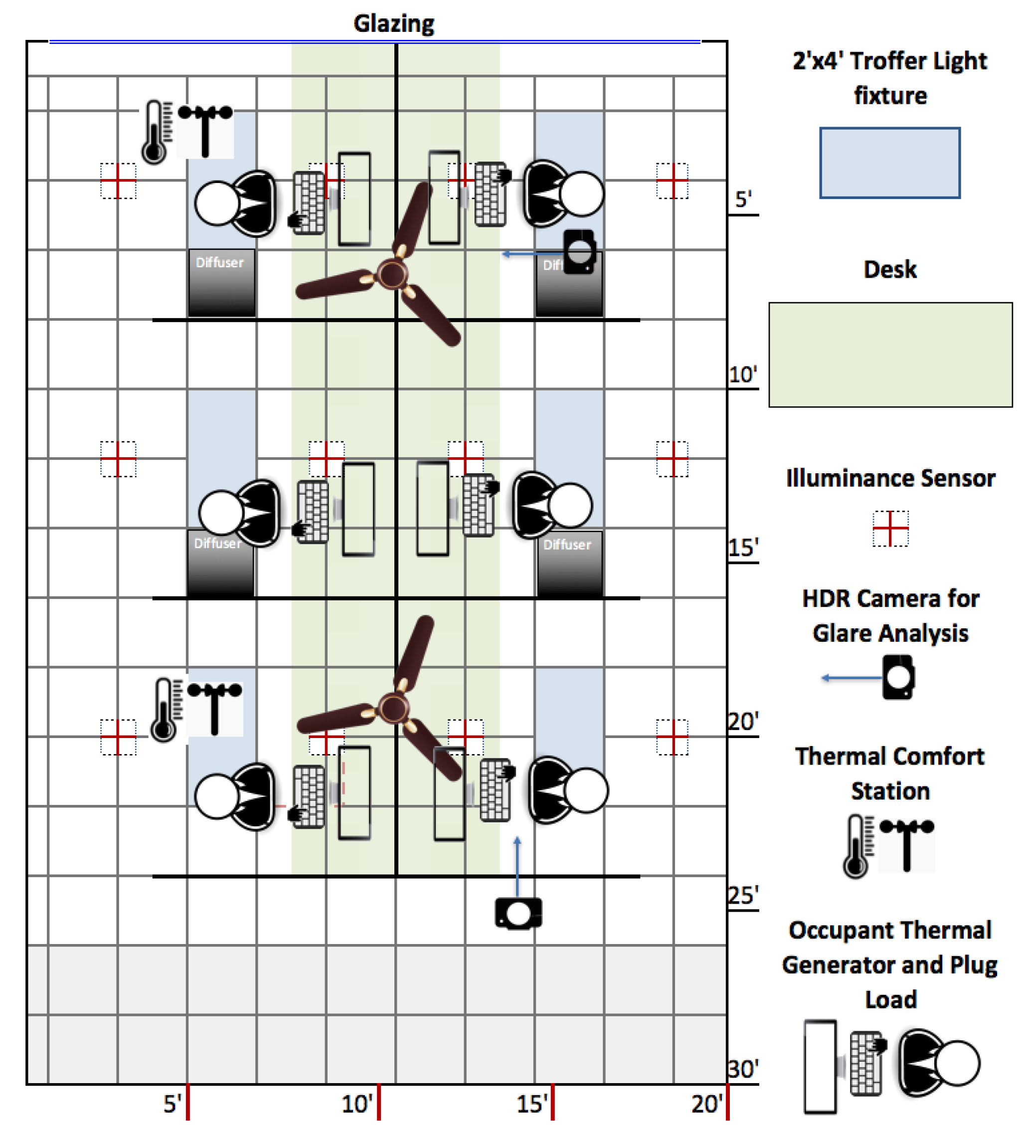
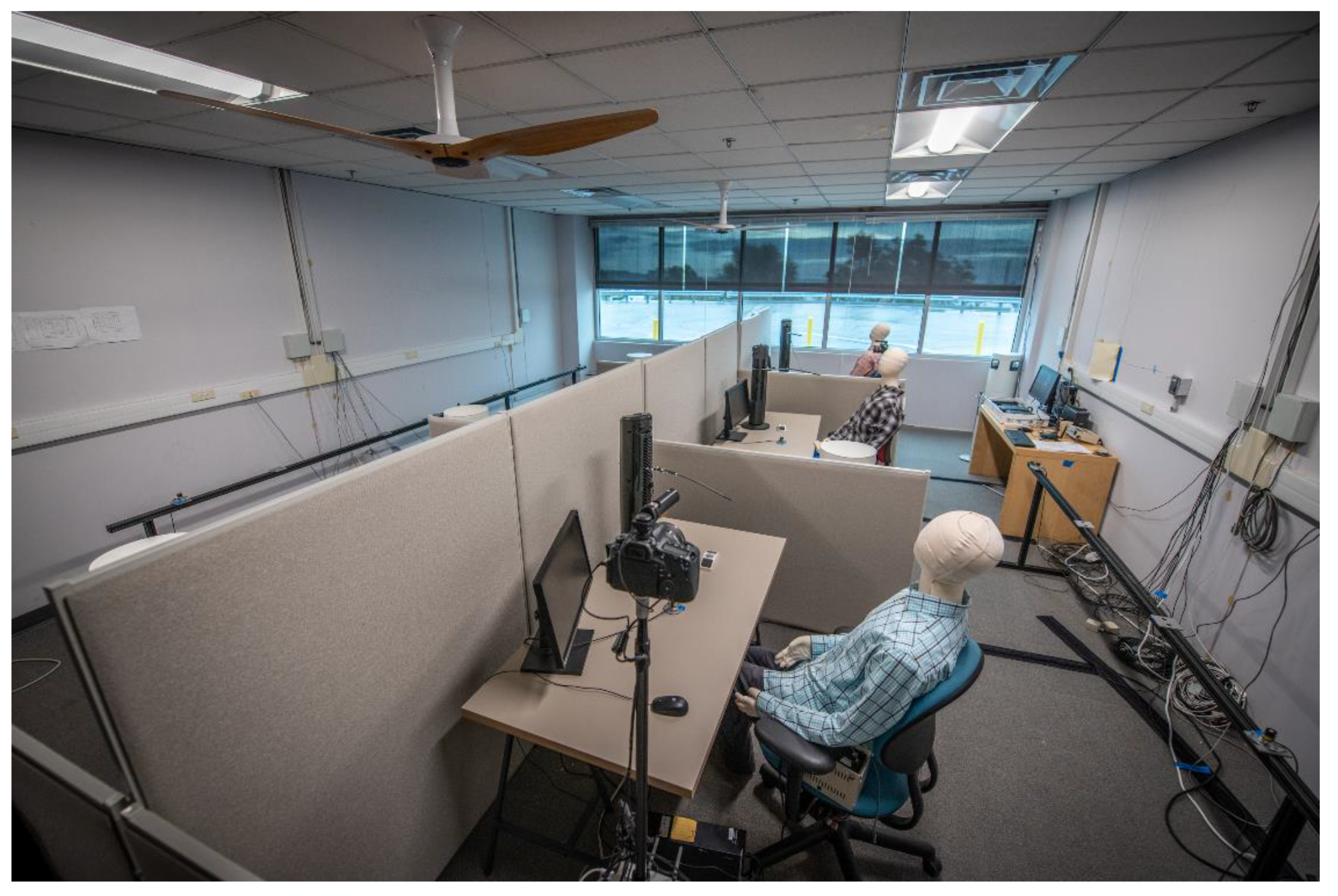
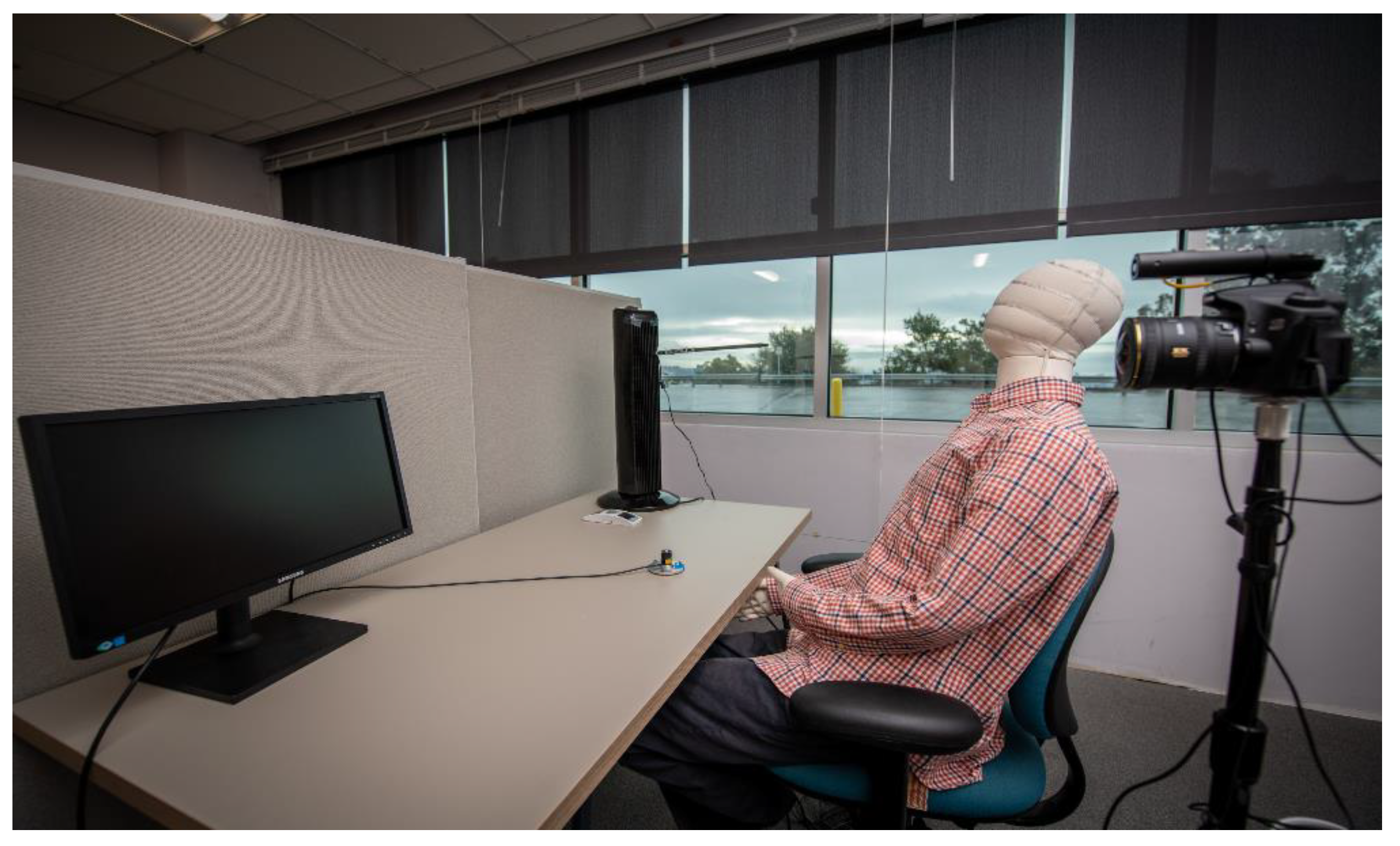
2.2. Laboratory Test Facility
2.3. Test Conditions for Reference and Test Cases
- supply air temperature (SAT) and duct static pressure reset (“trim and respond”);
- intermittent ventilation;
- economizing, with an outside air high-limit set to 23.9 °C (75 F);
- VAV minimum flow rate re-tuned, from 30% to around 15% (56.6 l/s (120 cfm));
- demand controlled ventilation based on occupancy status relayed by the lighting controls system.
2.4. Sensors and Measurements
2.5. Configurations Tested
3. Results and Discussion
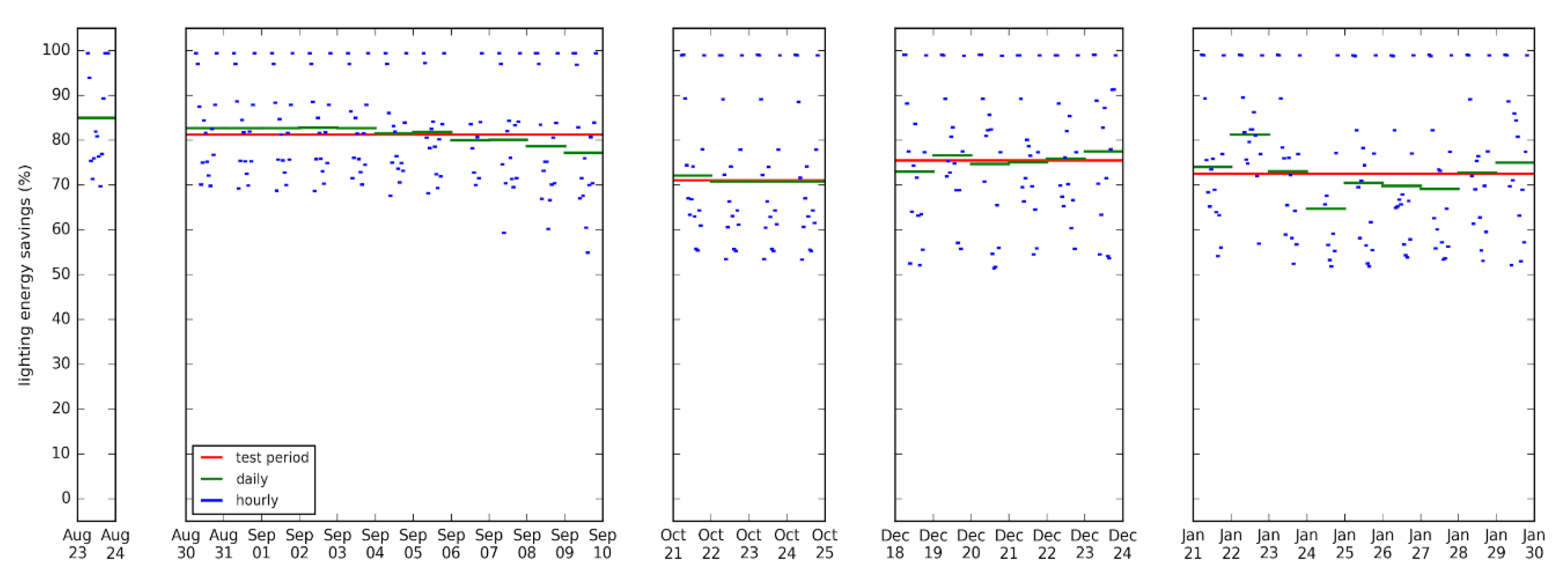
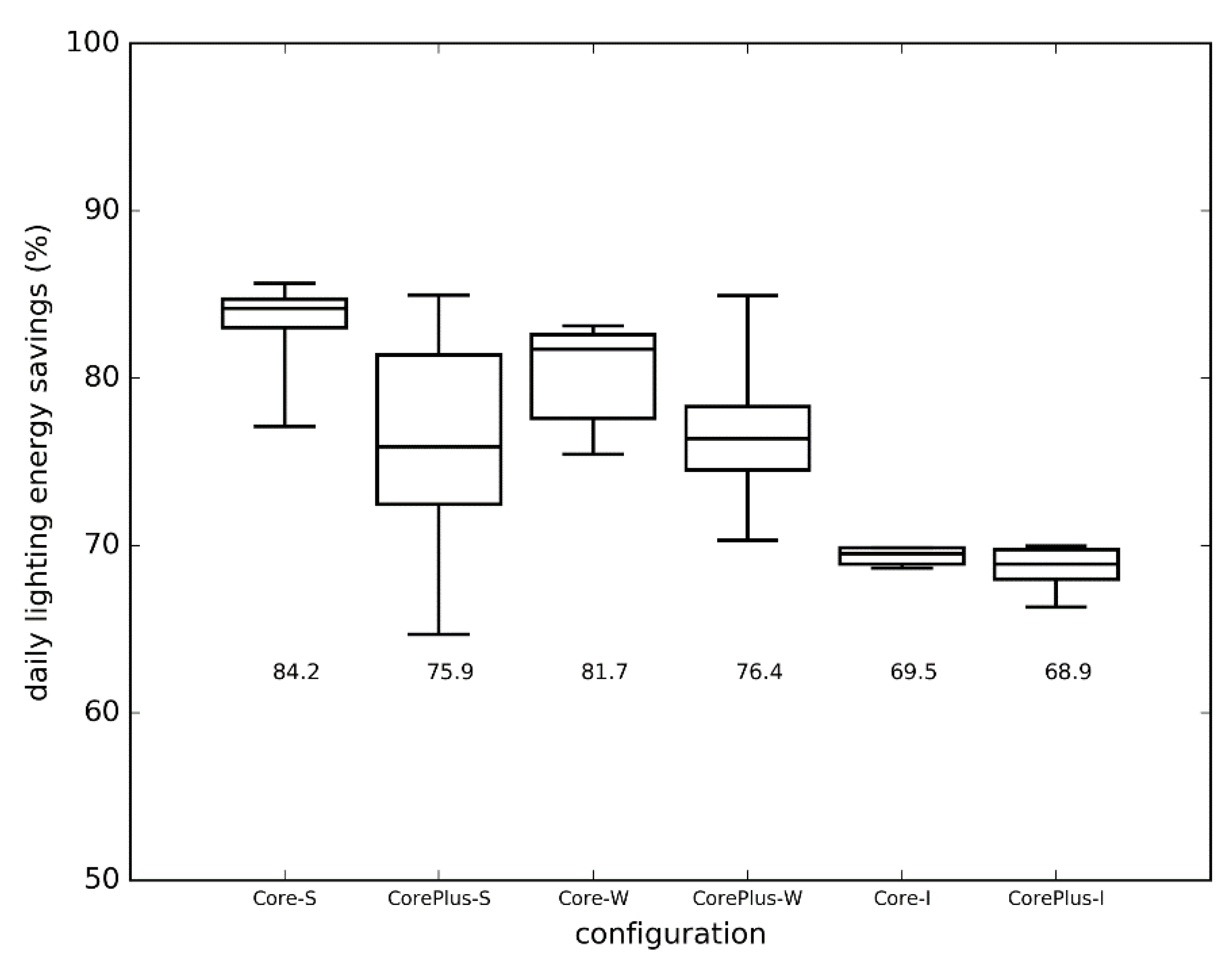
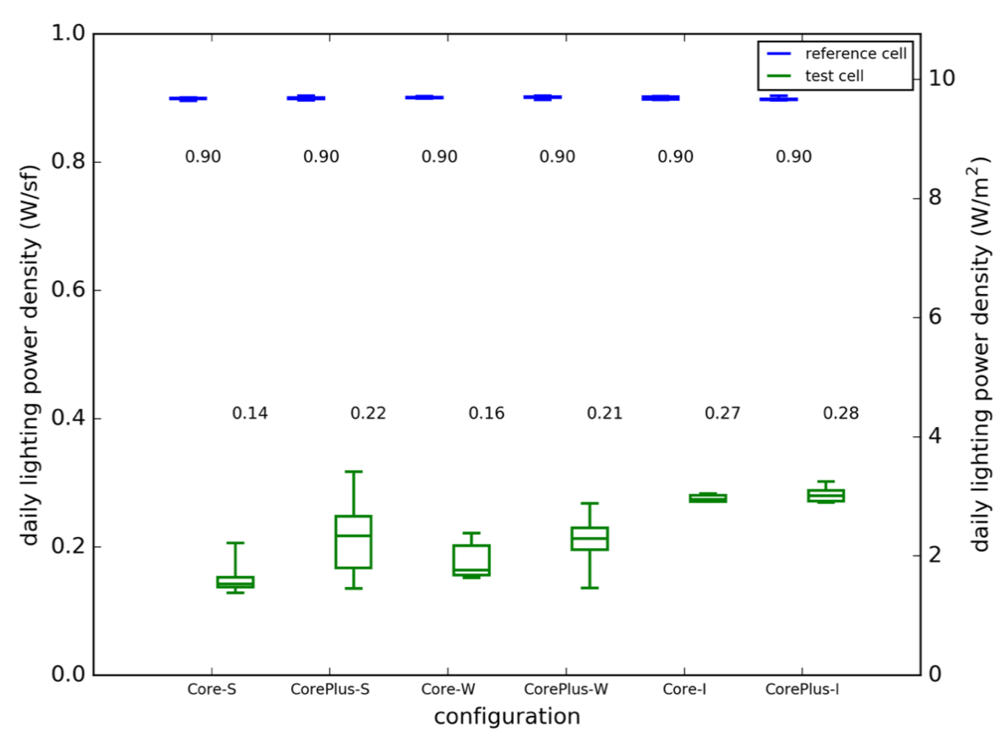
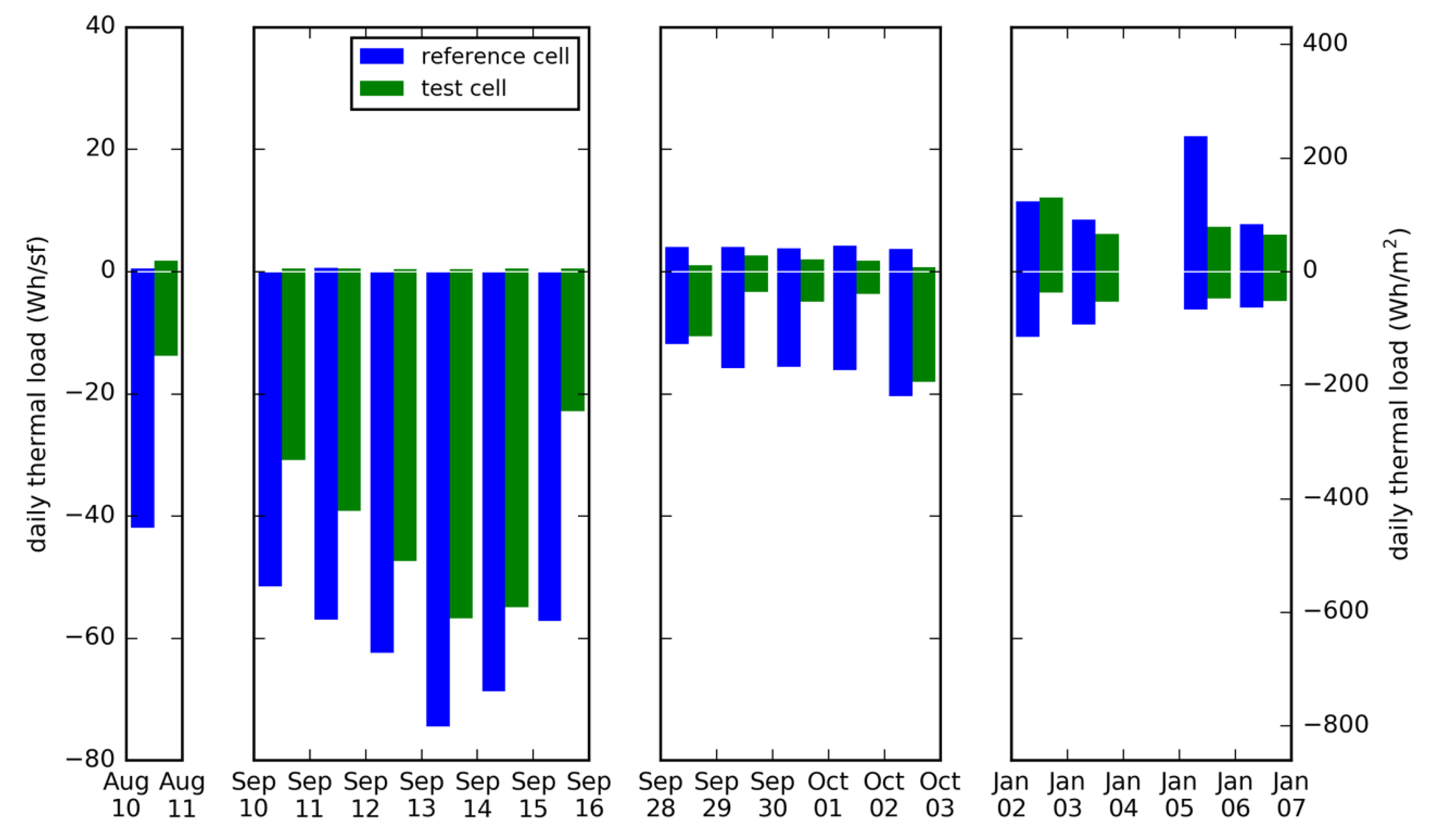
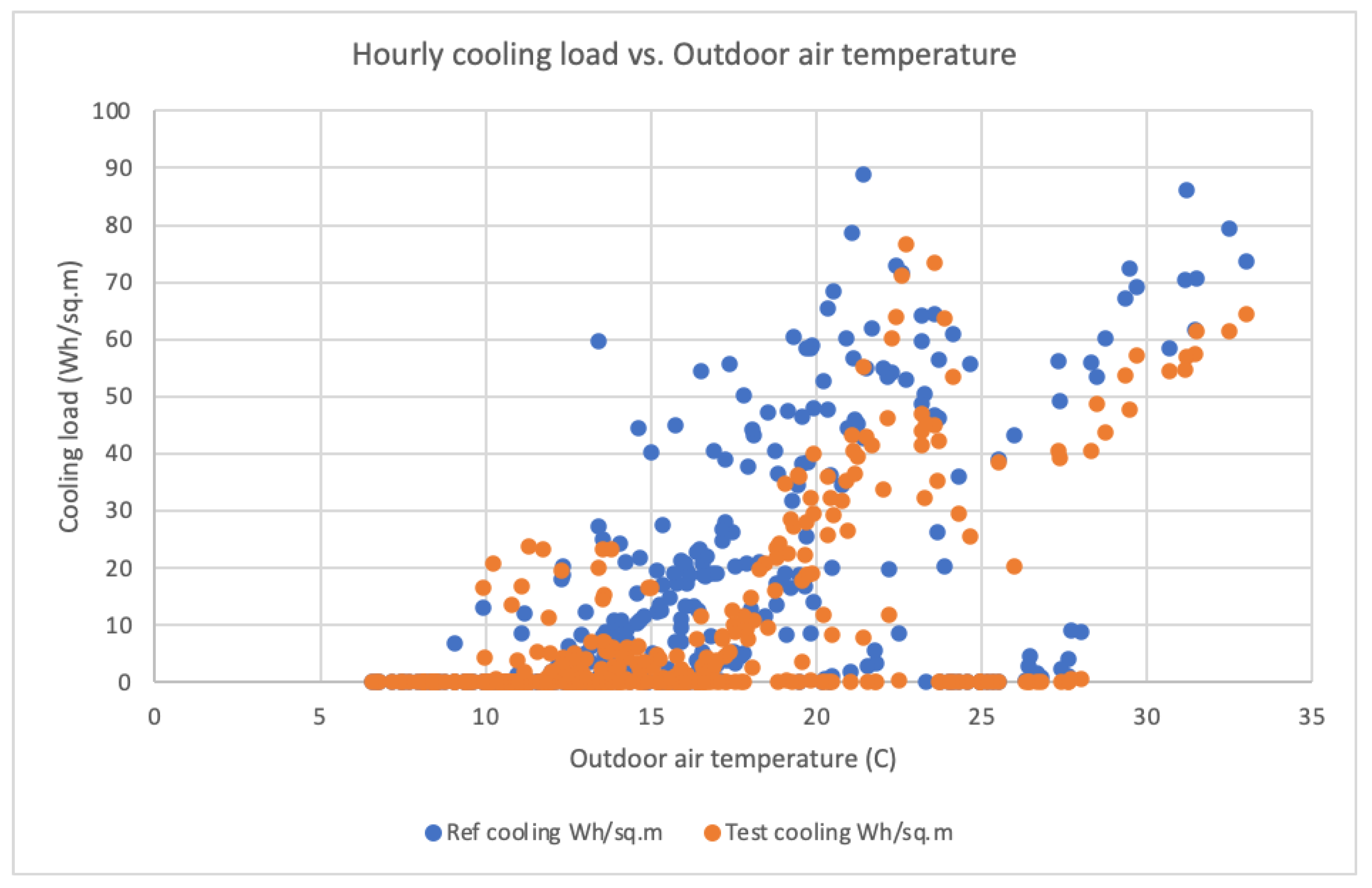
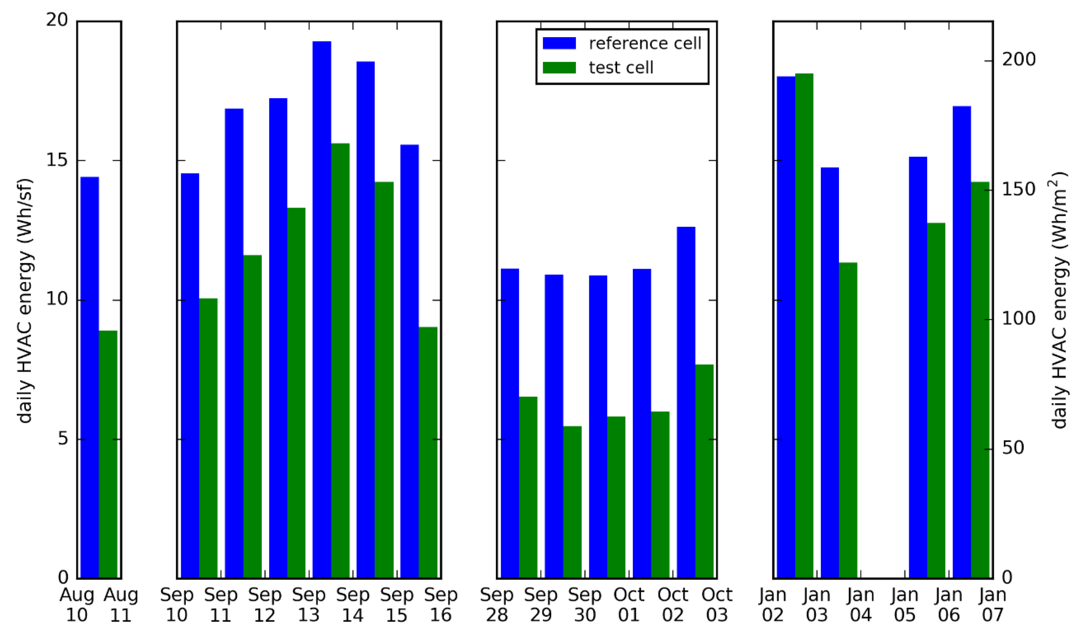
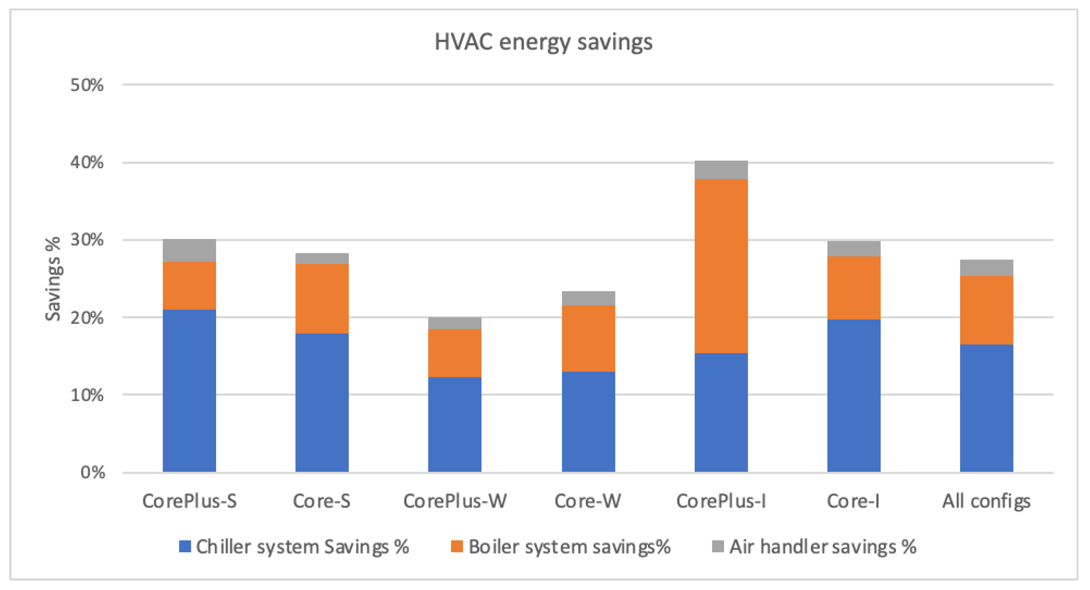
3.1. Energy Savings
3.1.1. Lighting
3.1.2. HVAC
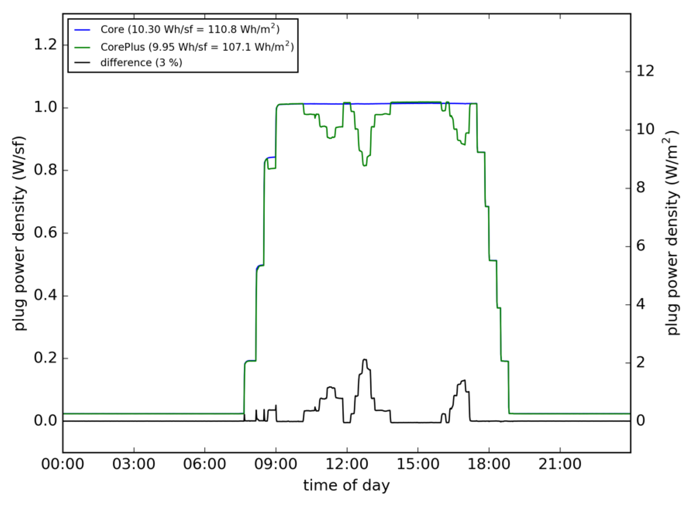
3.1.3. Plug Loads
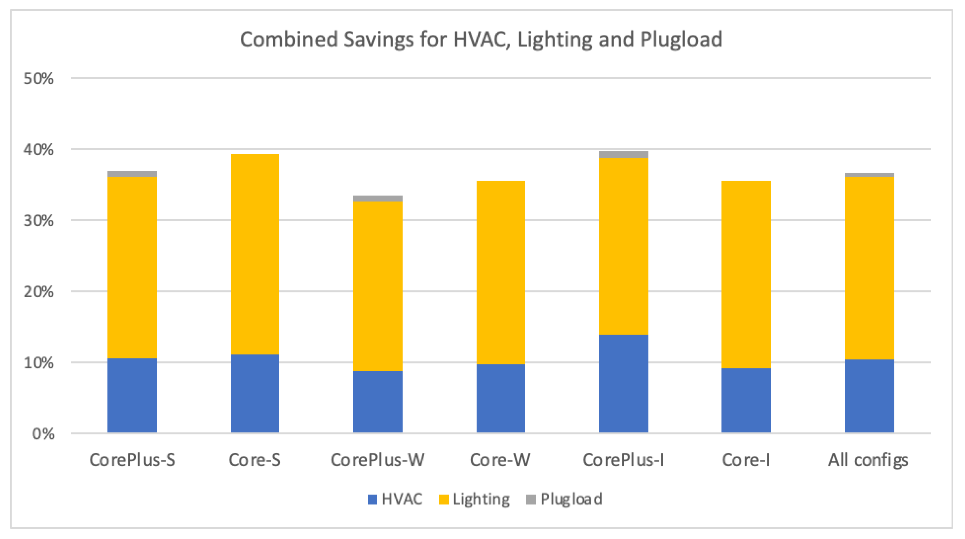
3.1.4. Combined Savings Estimates
3.2. Indoor Environmental Quality
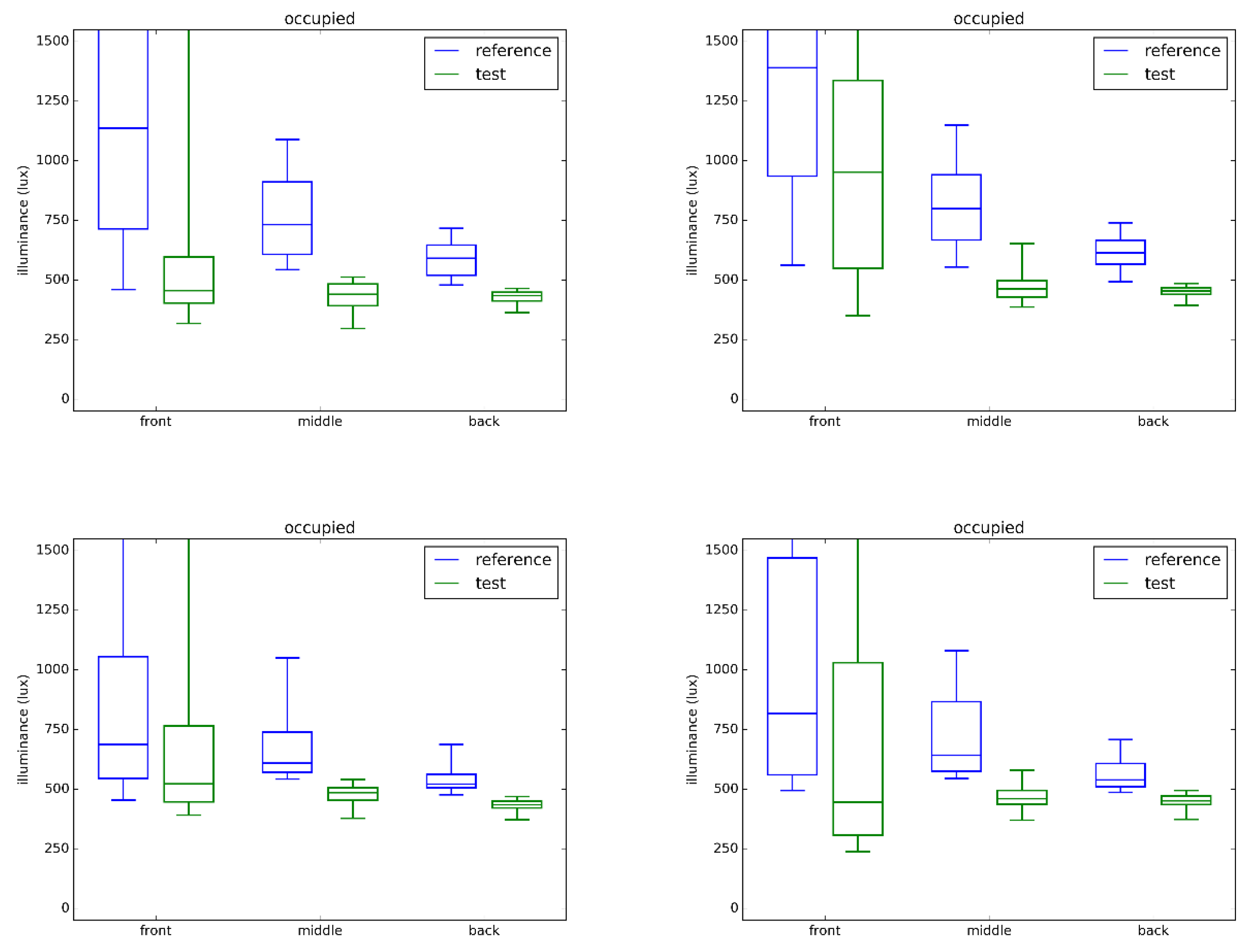
3.2.1. Illuminance
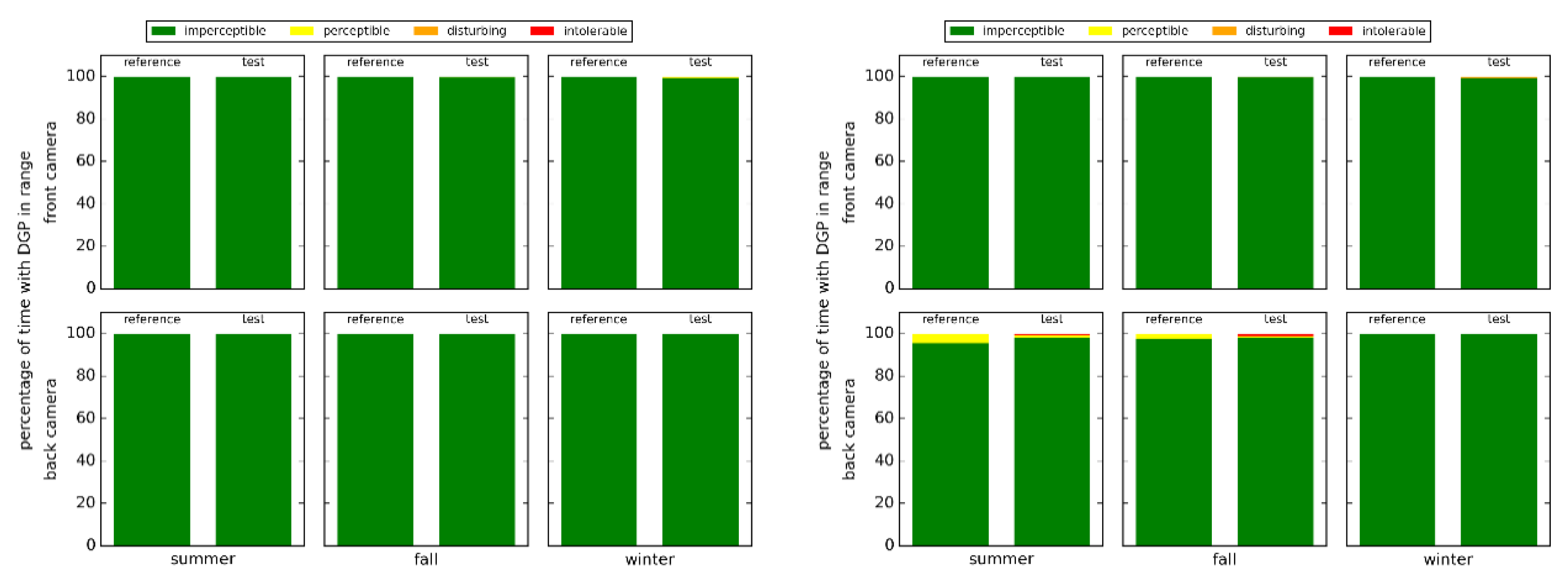
3.2.2. Daylight Glare Probability (DGP)
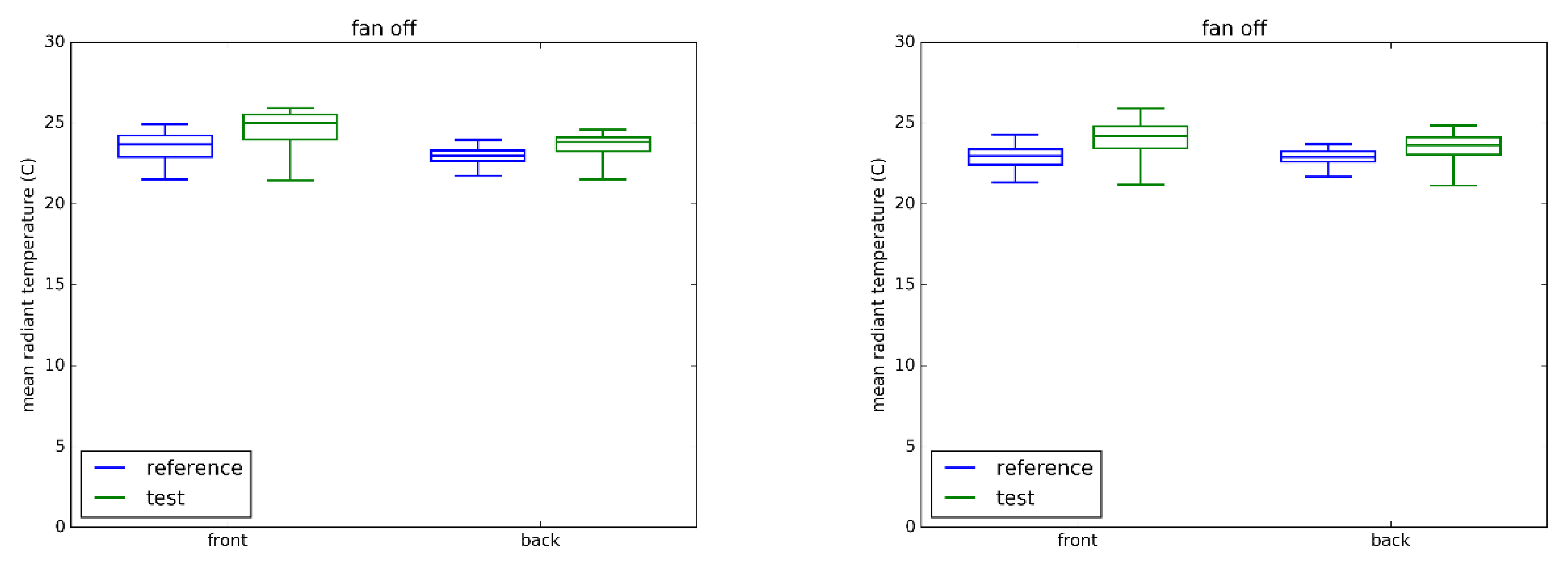
3.2.3. Mean Radiant Temperature
3.3. Installation, Commissioning and Operation
3.3.1. Lighting and HVAC Integration
3.3.2. ASHRAE G36 Controls
3.3.3. Ceiling Fan Controls Integration
3.3.4. Plug Load Controls
4. Conclusions
Supplementary Materials
Author Contributions
Funding
Acknowledgments
Conflicts of Interest
References
- Energy Information Administration (EIA)–Commercial Buildings Energy Consumption Survey (CBECS) Data. Available online: https://www.eia.gov/consumption/commercial/data/2012/ (accessed on 14 September 2020).
- Feierman, A. What’s in a Green Lease? Measuring the Potential Impact of Green Leases in the U.S. Office Sector; Institute for Market Transformation: Washington, DC, USA, 2015. [Google Scholar]
- Amann, J. Unlocking Ultra-Low Energy Performance in Existing Buildings; American Council for an Energy Efficient Economy: Washington, DC, USA, 2017. [Google Scholar]
- Kwatra, S.; Essig, C. The Promise and Potential of Comprehensive Commercial Building Retrofit Programs; American Council for an Energy Efficient Economy: Washington, DC, USA, 2014. [Google Scholar]
- Nadel, S.; Hinge, A. Mandatory Building Performance Standards: A Key Policy for Achieving Climate Goals; American Council for an Energy Efficient Economy: Washington, DC, USA, 2020. [Google Scholar]
- Navigant Energy Efficiency Retrofits for Commercial and Public Buildings. Navigant Consulting Inc., 2014. Available online: https://guidehouseinsights.com/reports (accessed on 12 October 2020).
- Zhai, J.; LeClaire, N.; Bendewald, M. Deep energy retrofit of commercial buildings: A key pathway toward low-carbon cities. Carb. Manag. 2011, 2, 425–430. [Google Scholar] [CrossRef]
- Granade, H.C.; Creyts, J.; Derkach, A.; Farese, P.; Nyquist, S. Unlocking Energy Efficiency in the U.S. Economy; McKinsey & Company: New York, NY, USA, 2009. [Google Scholar]
- PNNL; PECI. Advanced Energy Retrofit Guide–Office Buildings; Pacific Northwest National Laboratory: Washington, DC, USA, 2011. [Google Scholar]
- RMI Deep Energy Retrofits Using Energy Savings Performance Contracts: Success Stories. Available online: https://rmi.org/wp-content/uploads/2017/05/Deep-Energy-Retrofits-Using-ESPC-2015.pdf (accessed on 6 October 2020).
- Regnier, C.; Sun, K.; Hong, T.; Piette, M.A. Quantifying the benefits of a building retrofit using an integrated system approach: A case study. Energy Build. 2018, 159, 332–345. [Google Scholar] [CrossRef] [Green Version]
- Che, W.W.; Tso, C.; Sun, L.; Ip, D.Y.; Lee, H.; Chao, C.Y.; Lau, A.K.H. Energy consumption, indoor thermal comfort and air quality in a commercial office with retrofitted heat, ventilation and air conditioning (HVAC) system. Energy Build. 2019, 201, 202–215. [Google Scholar] [CrossRef]
- Regnier, C.; Mathew, P.A.; Robinson, A.; Shackelford, J.; Walter, T. Systems Retrofit Trends in Commercial Buildings: Opening Up Opportunities for Deeper Savings; Lawrence Berkeley National Laboratory: Beijing, China, 2020. [Google Scholar]
- RMI Deep Retrofit Tools and Resources. Available online: https://rmi.org/our-work/buildings/deep-retrofit-tools-resources/ (accessed on 6 October 2020).
- Lee, S.H.; Hong, T.; Piette, M.A.; Sawaya, G.; Chen, Y.; Taylor-Lange, S.C. Accelerating the energy retrofit of commercial buildings using a database of energy efficiency performance. Energy 2015, 90, 738–747. [Google Scholar] [CrossRef] [Green Version]
- Costa, J.F.W.; Amorim, C.N.D.; Silva, J.C.R. Retrofit guidelines towards the achievement of net zero energy buildings for office buildings in Brasilia. J. Build. Eng. 2020, 32, 101680. [Google Scholar] [CrossRef]
- Jungclaus, M.; Petersen, A.; Carmichael, C. Best Practices for Achieving Zero Over Time for Building Portfolios; Rocky Mountain Institute: Basalt, CO, USA, 2018. [Google Scholar]
- ULI Tenant Energy Optimization Program. Available online: https://tenantenergy.uli.org/10-steps-savings/ (accessed on 14 September 2020).
- Green Leasing Resources. Available online: https://www.greenleaseleaders.com/green-leasing-resources/ (accessed on 14 September 2020).
- Carmichael, C.; Petersen, A. Best Practices for Leased Net-Zero Energy Buildings: An Actionable Guide Explaining the Business Case and Process for Developers and Landlords to Pursue Net-Zero Energy Leased Buildings; Rocky Mountain Institute: Basalt, CO, USA, 2018. [Google Scholar]
- Davis, J.; Cloutier, D.; Ives, D.; Jewell, M.; Klein, A.; Tomey, V. Embedding Energy Efficiency in the Business of Buildings: Commercial Real Estate Contracts & Transactions; American Council for an Energy Efficient Economy: Washington, DC, USA, 2010. [Google Scholar]
- NYSERDA Commercial Tenant Program Case Studies. Available online: https://www.nyserda.ny.gov/All-Programs/Programs/Commercial-Tenant-Program/Resources (accessed on 14 September 2020).
- Mathew, P.; Coleman, P.; Page, J.; Regnier, C.; Shackelford, J.; Hopkins, G.; Jungclaus, M.; Olgyay, V. Energy Efficiency and the Real Estate Lifecycle: Stakeholder Perspectives; Office of Scientific and Technical Information (OSTI): Elza, TN, USA, 2019. [Google Scholar]
- Shackelford, J.; Mathew, P.A.; Regnier, C.; Walter, T. Laboratory Validation of Integrated Lighting Systems Retrofit Performance and Energy Savings. Energies 2020, 13, 3329. [Google Scholar] [CrossRef]
- Roisin, B.; Bodart, M.; Deneyer, A.; D’Herdt, P. Lighting energy savings in offices using different control systems and their real consumption. Energy Build. 2008, 40, 514–523. [Google Scholar] [CrossRef]
- Granderson, J.; Gaddam, V.; DiBartolomeo, D.; Li, X.; Rubinstein, F.; Das, S. Field-Measured Performance Evaluation of a Digital Daylighting System. LEUKOS 2010, 7, 85–101. [Google Scholar] [CrossRef]
- Williams, A.; Atkinson, B.; Garbesi, K.; Page, E.; Rubinstein, F. Lighting Controls in Commercial Buildings. LEUKOS 2012, 8, 161–180. [Google Scholar] [CrossRef]
- Fernandes, L.L.; Lee, E.S.; DiBartolomeo, D.L.; McNeil, A. Monitored lighting energy savings from dimmable lighting controls in The New York Times Headquarters Building. Energy Build. 2014, 68, 498–514. [Google Scholar] [CrossRef] [Green Version]
- ASHRAE. Guideline 36–2018. High-Performance Sequences of Operation for HVAC Systems; ASHRAE, 2018; Available online: https://www.techstreet.com/ashrae/standards/guideline-36-2018-high-performance-sequences-of-operation-for-hvac-systems?product_id=2016214 (accessed on 9 September 2020).
- He, Y.; Chen, W.; Wang, Z.; Zhang, H. Review of fan-use rates in field studies and their effects on thermal comfort, energy conservation, and human productivity. Energy Build. 2019, 194, 140–162. [Google Scholar] [CrossRef] [Green Version]
- Present, E.K.; Raftery, P.; Brager, G.; Graham, L.T. Ceiling fans in commercial buildings: In situ airspeeds & practitioner experience. Build. Environ. 2019, 147, 241–257. [Google Scholar] [CrossRef]
- FLEXLAB. Available online: https://flexlab.lbl.gov/ (accessed on 14 September 2020).
- Commercial Reference Buildings. Available online: https://www.energy.gov/eere/buildings/commercial-reference-buildings (accessed on 14 September 2020).
- ASHRAE. Standard 90.1 Energy Standard for Buildings Except Low-Rise Residential Buildings; ASHRAE, 2019; Available online: https://www.ashrae.org/technical-resources/bookstore/standard-90-1 (accessed on 14 September 2020).
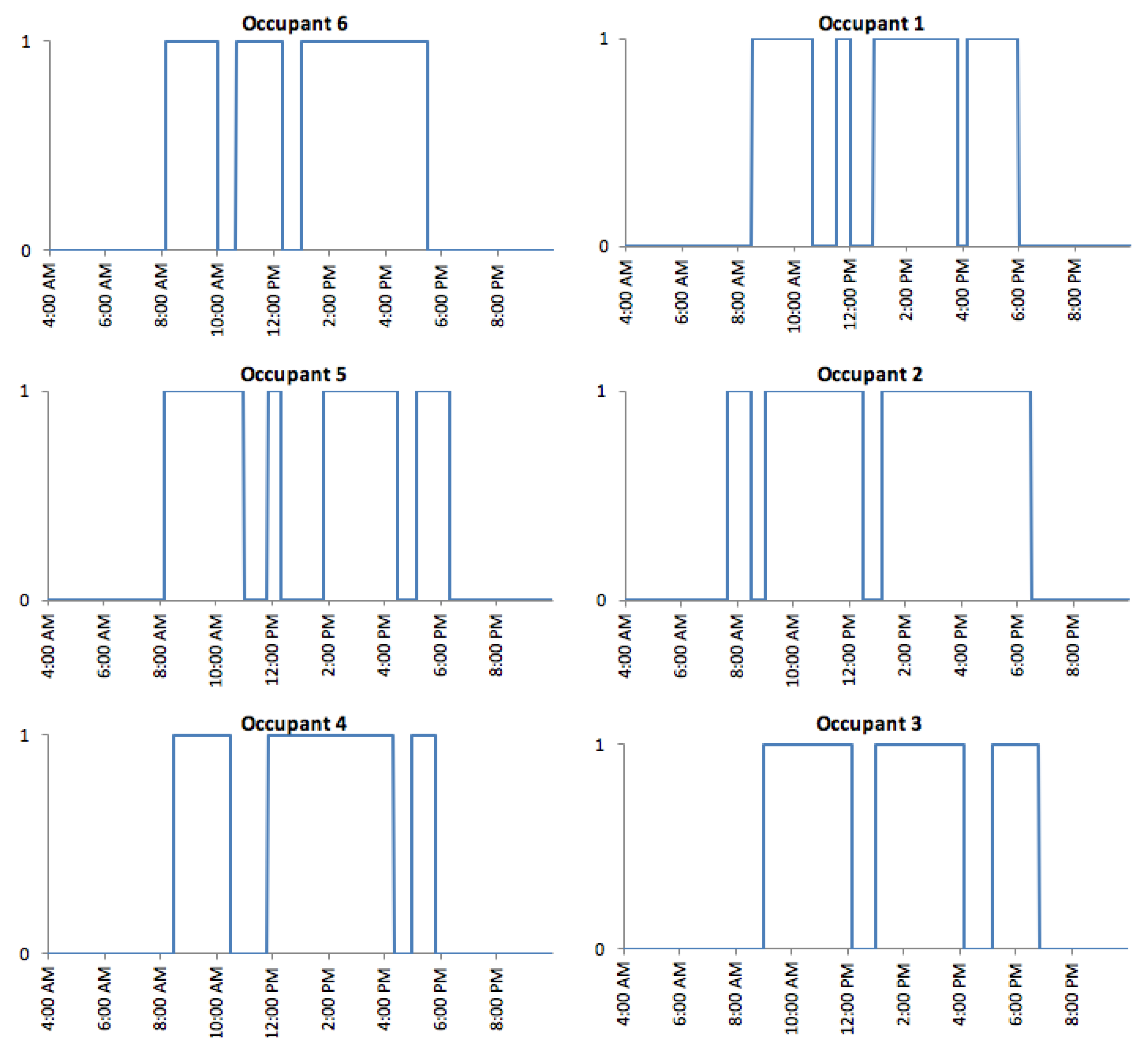
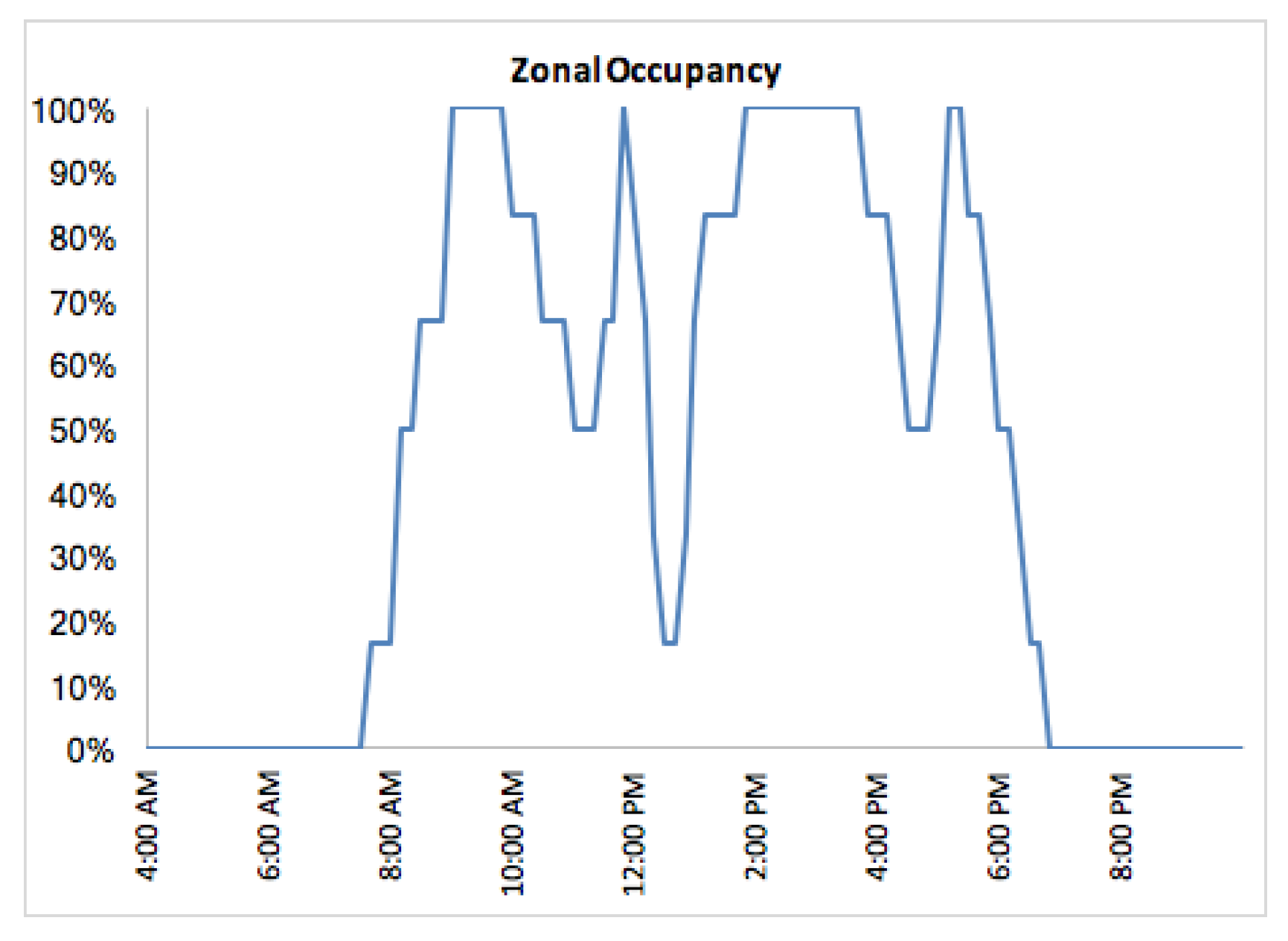
- Chen, Y.; Hong, T.; Luo, X. An agent-based stochastic Occupancy Simulator. Build. Simul. 2017, 11, 37–49. [Google Scholar] [CrossRef]
- Commercial Prototype Building Models. Available online: https://www.energycodes.gov/development/commercial/prototype_models (accessed on 14 September 2020).
- Haleem, S.M.A.; Pavlak, G.S.; Bahnfleth, W.P. Performance of advanced control sequences in handling uncertainty in energy use and indoor environmental quality using uncertainty and sensitivity analysis for control components. Energy Build. 2020, 225, 110308. [Google Scholar] [CrossRef]


| Measure | ⚫ Core ◯ Optional |
|---|---|
| Lighting | |
| LED Fixtures | ⚫ |
| Occupancy-based controls | ⚫ |
| Daylight dimming controls | ⚫ |
| Network lighting controls system | ◯ |
| HVAC | |
| ASHRAE Guideline 36 Controls (trim & respond for supply air temp and duct static pressure, demand-controlled ventilation, intermittent ventilation, VAV box retuning) | ⚫ |
| Ceiling fans w/2.2 °C (4 F) cooling setback | ◯ |
| Other | |
| Automated interior Shades | ◯ |
| Plug load controls | ◯ |
| Metering & monitoring | ⚫ |
| System | Feature | Reference Cell | Test Cell: Core | Test Cell: CorePlus |
|---|---|---|---|---|
| Lighting | Fixtures | 3-lamp T8 fluorescent troffer | LED troffer with integrated sensors and controls | LED troffer with integrated sensors and controls |
| Controls | Scheduled on/off (6 a.m. to 8 p.m.) | Fixture-level occupancy-based dimming, afterhours shut off, fixture-level daylight dimming. Occupancy data shared with HVAC via API. | Fixture-level occupancy-based dimming, afterhours shut off, fixture-level daylight dimming. Occupancy data shared with HVAC via API. | |
| HVAC | System type | VAV Air handling unit with hydronic cooling and heating; VAV with hydronic reheat (emulated) | same | same |
| Heating and cooling setpoints, schedule | Occupied: 21.1 °C/23.3 °C (70 F/74 F) (hours: 7 a.m.–7 p.m.) Unoccupied setback: 15.6 °C/29.4 °C (60 F/85 F) 2-h morning warmup or cooldown based on t-stat and setpoints. | Same heating and cooling setpoints. Same schedule. Morning warmup/cooldown (varies by season: 0.5 h for summer, 1 h for spring/fall, and 1.5 h for winter, conditioning based on t-stat and setpoints). | Same heating and cooling setpoints. Same schedule. Morning warmup/cooldown (varies by season: 0.5 h for summer, 1 h for spring/fall, and 1.5 h for winter, conditioning based on t-stat and setpoints). Automated ceiling fans (on once zone in cooling mode for 1 h, cooling setpoint setback of 2.2 °C (4 F)) | |
| Supply air temp (SAT), VAV min flow | Cooling SAT: 55 F (12.8 °C) (no reset). VAV minimum flow set to 30%, 106 l/s (225 cfm). | SAT reset per ASHRAE Guideline 36, (“trim and respond”). VAV min flow tuned to 15%, 57 l/s (120 cfm). | SAT reset per ASHRAE Guideline 36, (“trim and respond”). VAV min flow tuned to 15%, 57 l/s (120 cfm). | |
| Ventilation | Standard ventilation amount per ASHRAE Standard 62-2016. Does not turn off after hours; outside air damper maintains same position as occupied condition | Standard ventilation amount per ASHRAE Standard 62-2016. Demand controlled ventilation per ASHRAE Guideline 36, based on occupancy % for zone, calculated from lighting system data. Can turn down to zero flow off hours. Intermittent ventilation: 15 min ‘on’ as min supply period, cycles on/off when in minimum flow to provide overall total vent amount needed. | Standard ventilation amount per ASHRAE Standard 62-2016. Demand controlled ventilation per ASHRAE Guideline 36, based on occupancy % for zone, calculated from lighting system data. Can turn down to zero flow off hours. Intermittent ventilation: 15 min ‘on’ as min supply period, cycles on/off when in minimum flow to provide overall total vent amount needed. | |
| Economizer | Temp based, with 18.3 °C (65 F) high limit cutoff. No econ prior to 28 September 2019. | Operation per ASHRAE Guideline 36; outside air high limit cutoff 23.9 °C (75 F). | Operation per ASHRAE Guideline 36; outside air high limit cutoff 23.9 °C (75 F). | |
| Plug Loads | Wattage and operation | Approx. 100 W per workstation (CPU and monitor) on during workday | Same | Same |
| Controls | None | None | Occupancy—based turn off of monitor after 5 min timeout for occupancy sensor | |
| Windows | Glazing | Double-pane tinted U-value of 0.594, SHGC 0.41, vis trans 0.276 | Same | Same |
| Shading | Venetian blinds, seasonally adjusted louver angle adjustment | Venetian blinds, seasonally adjusted louver angle adjustment | Automated rollershades controlled based on solar position and sky condition | |
| Exterior Walls | Wall insulation | Metal stud with R-19 batt insulation and drywall, exterior has cementitious board. | Same | Same |
| Configuration ID | Configuration Details |
|---|---|
| Core-S | Core measures only, south-facing window wall |
| Core-W | Core measures only, west-facing window wall |
| Core-I | Core measures only, interior zone (no window wall) |
| CorePlus-S | Core measures plus optional measures, south-facing window wall |
| CorePlus-W | Core measures plus optional measures, west-facing window wall |
| CorePlus-I | Core measures plus optional measures, interior zone (no window wall) |
| Config | Days per Month per Configuration | Total Days | |||||
|---|---|---|---|---|---|---|---|
| Aug | Sep | Oct | Nov | Dec | Jan | ||
| Core-S | 1 | 9 | 2 | 4 | 16 | ||
| Core-W | 4 | 5 | 2 | 7 | 18 | ||
| Core-I | 4 | 5 | 9 | ||||
| CorePlus-S | 4 * | 6 | 4 | 6 | 7 | 27 | |
| CorePlus-W | 4 | 5 | 6 | 15 | |||
| CorePlus-I | 6 | 5 | 11 | ||||
| Configuration | Cooling Load Savings % | Heating Load Savings % | HVAC Energy Use Savings % |
|---|---|---|---|
| CorePlus-S | 54% | 25% | 30% |
| Core-S | 38% | 37% | 28% |
| CorePlus-W | 52% | 4% | 20% |
| Core-W | 42% | 10% | 23% |
| CorePlus-I | 47% | 54% | 40% |
| Core-I | 62% | 32% | 30% |
| All configs | 48% | 23% | 27% |
| Configuration | Lighting Energy Savings (% of All Three End Uses) | HVAC Energy Savings (% of All Three End Uses) | Plug Load Energy Savings (% of All Three End Uses) | Combined Energy Savings (% of All Three End Uses) |
|---|---|---|---|---|
| CorePlus-S | 26% | 11% | 1% | 37% |
| Core-S | 28% | 11% | 0% | 39% |
| CorePlus-W | 24% | 9% | 1% | 33% |
| Core-W | 26% | 10% | 0% | 36% |
| CorePlus-I | 25% | 14% | 1% | 40% |
| Core-I | 26% | 9% | 0% | 36% |
| All configs | 26% | 10% | 0% | 37% |
© 2020 by the authors. Licensee MDPI, Basel, Switzerland. This article is an open access article distributed under the terms and conditions of the Creative Commons Attribution (CC BY) license (http://creativecommons.org/licenses/by/4.0/).
Share and Cite
Mathew, P.; Regnier, C.; Shackelford, J.; Walter, T. Energy Efficiency Package for Tenant Fit-Out: Laboratory Testing and Validation of Energy Savings and Indoor Environmental Quality. Energies 2020, 13, 5311. https://0-doi-org.brum.beds.ac.uk/10.3390/en13205311
Mathew P, Regnier C, Shackelford J, Walter T. Energy Efficiency Package for Tenant Fit-Out: Laboratory Testing and Validation of Energy Savings and Indoor Environmental Quality. Energies. 2020; 13(20):5311. https://0-doi-org.brum.beds.ac.uk/10.3390/en13205311
Chicago/Turabian StyleMathew, Paul, Cindy Regnier, Jordan Shackelford, and Travis Walter. 2020. "Energy Efficiency Package for Tenant Fit-Out: Laboratory Testing and Validation of Energy Savings and Indoor Environmental Quality" Energies 13, no. 20: 5311. https://0-doi-org.brum.beds.ac.uk/10.3390/en13205311