Article

A Novel Application of Improved Marine Predators Algorithm and Particle Swarm Optimization for Solving the ORPD Problem

1
Electrical Engineering Department, Faculty of Engineering and Technology, Future University in Egypt, Cairo 11835, Egypt
2
Electrical Engineering Department, Faculty of Engineering, Fayoum University, Fayoum 63514, Egypt
3
Electrical Engineering Department, Faculty of Engineering, Jouf University, Sakakah 74331, Saudi Arabia
4
Electrical Power and Machine Department, Faculty of Engineering, Zagazig University, Zagazig 44519, Egypt
5
Department of Electrical Engineering, College of Engineering, King Saud University, P.O. Box 800, Riyadh 11421, Saudi Arabia
6
School of Electrical Engineering Computing and Mathematical Sciences, Curtin University, Perth 6102, Australia
*
Author to whom correspondence should be addressed.
Submission received: 9 October 2020 / Revised: 25 October 2020 / Accepted: 26 October 2020 / Published: 30 October 2020
(This article belongs to the Section F: Electrical Engineering)

Abstract

:
The appropriate planning of electric power systems has a significant effect on the economic situation of countries. For the protection and reliability of the power system, the optimal reactive power dispatch (ORPD) problem is an essential issue. The ORPD is a non-linear, non-convex, and continuous or non-continuous optimization problem. Therefore, introducing a reliable optimizer is a challenging task to solve this optimization problem. This study proposes a robust and flexible optimization algorithm with the minimum adjustable parameters named Improved Marine Predators Algorithm and Particle Swarm Optimization (IMPAPSO) algorithm, for dealing with the non-linearity of ORPD. The IMPAPSO is evaluated using various test cases, including IEEE 30 bus, IEEE 57 bus, and IEEE 118 bus systems. An effectiveness of the proposed optimization algorithm was verified through a rigorous comparative study with other optimization methods. There was a noticeable enhancement in the electric power networks behavior when using the IMPAPSO method. Moreover, the IMPAPSO high convergence speed was an observed feature in a comparison with its peers.

1. Introduction

The electrical power system is a complex system consisting of subsystems, such as generation plants and transmission networks. Therefore, the performance of electric power systems needs to be controlled and evaluated in order to ensure proper and safe system operation. An important problem in power planning and operation is the Optimum Reactive Power Dispatch (ORPD). It has a great effect when studying how to operate the power system economically. Complex power is provided by the generation side, whereas active power is consumed by the demand side, and the reactive power keeps circulating through the network. However, the reactive power is important to keep the voltage within its stable limits. Additionally, reactive power is important for the transmission of the active power through the grid. Hence, the ORPD problem is an important aspect of power system operation.
Many parameters in the power systems are to be kept within certain limits, such as the voltage on the bus or power transmitted through a transmission line. Otherwise, any violation in these limits can lead to a system failure. As a result, these problems were solved by simulating and analyzing power systems, such as the optimal power flow (OPF) problem and the ORPD problem. In general, there are many objectives for the ORPD problem such as transmission cost minimization [1], active power loss minimization [2], improving the voltage profile [3], and voltage stability enhancement. Generally speaking, there are many variables that could be considered as control variables for the ORPD optimization problem, such as the voltages at the generating units, transformer tap settings, and the buses at which the shunt reactive power compensators could be placed. After solving this optimization problem, its constraints must be rechecked to assure that they are already kept within limits and there is no violation in the voltage or power values [4,5,6,7,8,9]. The optimal solution corresponds to the best fit control variables.
The ORPD problem was described through the use of many conventional optimization methods as non-linear and non-convex optimization problems [10,11,12,13,14,15]. Samples of these traditional tools are linear programming (LP) [10], interior point method [11], quadratic programming (QP) [12], and Newton-Raphson [13]. The traditional methods encountered many points that were considered to be weak points. They need many numerical iterations to finish the calculations. This, accordingly, leads to high computational time consumption. Lately, development is taking place and is continuing in the scope of the optimization tools. This resulted in the existence of many optimization techniques that were tested widely on various applications in the scope of optimization, especially in the field of power systems.
There are many meta-heuristic optimization methods used to optimally solve the ORPD. Sunflower optimization [16,17], hybrid firefly and particle swarm optimization [18], gravitational based search optimizer [19], brain storm optimization algorithm [20], tree seed algorithm [21], salp swarm optimization [22,23,24], sine-cosine algorithm [25], coyote optimization algorithm [26], seeker optimization algorithm [27], bacteria foraging optimization [28], cuckoo search algorithm [29,30,31], grasshopper optimization [32], Harris hawks optimization (HHO) [33], artificial bee colony (ABC) [34], gravitational search algorithm (GSA) [35], and the firefly algorithm [36], represent samples of the lately employed methods for the optimization problems. The genetic algorithm (GA) was utilized in [37], and the dynamic PSO was used in [38,39]. GA is fundamentally based on genetic dynamics concepts. The efficiency of such an approach depends mainly on adequate coding of the population. The first population is generated randomly at the beginning. Individuals in this population are seen as likely solutions to the problem of optimization. The progress of the simulation converts the population dynamics partly into future generations. In [40,41,42], GA was applied to the ORPD optimization problem. Differential evolution (DE) optimizer is also one of the optimization methods used in solving the ORPD. The advantage of the DE is that, it can be implemented easily and effectively [43]. Despite the effectiveness in solving the optimization problems, the optimal solutions might not be guaranteed every time they are used. One of the negative points of these strategies is that, they could be restricted to a minimal local. The fine tuning of the tool parameter also affects the convergence speed directly. The no-free-lunch theorem of the mathematical optimization proved that none-of them could be the best option for all possible optimization problems. However, there can be a better one for one specific task. Moreover, the firefly algorithm has a similar weakness as the marine predators and other such algorithm, which uses many iterations in a single step. These two things are summarized in [44]. Therefore, the hybrid evolutionary optimization methods were then introduced to overcome such disadvantages [45,46,47,48,49].
In this circumstance, improved meta-heuristic techniques and hybrid optimization techniques were then introduced and applied to the ORPD problem to find better solutions to the problem. In [50], a new modification was inserted to the sine-cosine algorithm and applied to the ORPD problem [45], which also introduced a hybrid modified imperialist competitive algorithm (MICA) and invasive weed optimization (IWO) for the same target. An enhancement was made to the firefly optimization algorithm to solve a multi-objective ORPD in [51]. More hybrid optimization techniques were proposed in [52,53,54,55,56,57,58,59]. In [52], the ORPD problem was solved using the hybrid GA and interior point method [53], which introduced a solution to the ORPD problem using hybrid artificial bee colony and differential evolution algorithm tested with the IEEE 14-bus, 30-bus, and 57-bus systems. Deferential Evolution itself needs a large number of agents to avoid premature settlement, which takes a long time. Moreover, the results were compared with DE itself. In [54], hybrid teaching learning and a double DE algorithm was proposed and applied to a single objective function, which is power losses minimization in the IEEE 14-, 30-, and 118-bus systems. Moreover, a comparison between the results were provided. In [55], modifications were made to the social spider optimization (SSO) method on how the algorithm generates new solutions. Then, this was used for solving the ORPD problem with the IEEE 30- and 118-bus systems. The weak point of the SSO itself was that it contains many control parameters, which increases the implementation complexity and execution time. Two single objective functions were studied. In [56], hybrid multi-swarm PSO was introduced to solve a multi-objective ORPD. The idea was that, each swarm was divided into sub-swarms, then a PSO was used as a search engine for the sub-swarms. Additionally, the DE method was used to enhance the best of the particles themselves. The studied systems were the IEEE 30-bus and practical 75-bus Indian systems. In [57], ORPD was solved using a hybrid Nelder–Mead simplex and a firefly optimization method (FA). The weak point of the FA was the trapping into local optima. Two single objectives were studied; power loss minimization and voltage deviation minimization. The research was applied to the IEEE 30-, and 118-bus systems. In [59], ORPD was solved by the proposed modified NSGA-II algorithm. The problem was a multi-objective function, which minimized power loss, besides maximizing the voltage stability. The systems tested in that work were the IEEE 30- and 118- bus systems. The single objective function optimization problem focused only on getting the best solution for one target at a time. On the other hand, in the multi-objective optimization problems, more than one objective was to be targeted simultaneously. Accordingly, introducing a more flexible algorithm with minimal adjustable paragliders was the motivated key for developing a new hybrid algorithm.
The marine predators algorithm (MPA) is a population-based technique [60] that was inspired mainly by the foraging strategies of the ocean predators and their interactions with the prey. The MPA was applied to solve several optimization problems in the field of solar energy. The MPA was applied to large scale photovoltaic (PV) array reconfiguration [61] and for PV modeling [62,63]. Furthermore, the MPA confirmed an efficient performance for forecasting COVID19 cases [64]. The simplicity of MPA in the implementation attracted the researchers to examine it with their applications, whereas the MPAs main disadvantage was that, the number of iterations was divided between the main phases of the algorithm. Therefore, it required huge number of iterations, especially with nonlinear optimization problems. For solving this point, an improved version of the MPA was proposed, based on distribution and particle swarm optimization. As a result, an improved marine predators algorithm and particle swarm optimization (IMPAPSO) method was introduced in this study. This was a salient and new contribution of this research work.
This study introduces an inspection to the newly developed MPA with some modifications and hybridization between the MPA and PSO, in order to optimize the decision variables of the ORPD. The proposed algorithm was examined with three systems of the IEEE 30 bus, IEEE 57 bus, and IEEE 118 bus, and compared with recent reported techniques in literatures. The effectiveness of the IMPAPSO was verified as an optimization tool to be utilized in solving the problem of ORPD for three bus systems of the IEEE 30 bus, IEEE 57 bus, and IEEE 118 bus. Moreover, the proposed algorithm was performed competitively, in comparison with the MPA itself and other optimization tools. Therefore, the research study focused on selecting the best possible decision variables to achieve the lowest possible active power loss in the grid. This paper also demonstrated how the voltage of the PQ buses could be optimized. In this analysis, the competence of the proposed optimization methodology was verified by different test systems. The objective functions studied in this research are single ones.
The remaining parts of the manuscript are organized as follows. Section 2 describes the mathematical formula of the proposed objective function. The overview representation of the MPA and IMPAPSO was documented in Section 3. Section 4 presents the simulation and results, and finally, Section 5 summarizes the main outcomes and the future work.

2. Problem Formulation

Generally speaking, the ORPD target was to optimize a non-linear function [63]. The constraints must be guided within their maximum and minimum boundaries, through the process of optimization [65]. It could be represented mathematically by Equations (1) and (2):
Min   F ( x , u )
Subject   to :   g ( x , u )   =   0 , h ( x , u )     0
The symbol F is used to refer to the objective to be minimized. Meanwhile u and x are selected to refer to the preset control variables as well as the dependent variables.
There are three variables defined as control variables in this study. They are—(1) the voltage of the generator bus, (2) the tapping of the transformers, and finally, (3) the reactive power entering the studied electric power system from the VAR compensators. They are represented by Equations (3) and (4):
u T   =   [ V G 1 V G NGen , Q C 1 Q C NCom , T 1 T NTr ]
Additionally, the dependent variables are mathematically represented in Equation (4):
x T   =   [ V L 1 V L NLB , Q G 1 Q G NGen , S l 1 S l Nline ]
The ORPD objective function seeks the minimum active power losses. Additionally, the constraints must be considered during the simulation process. The optimal solution was found by varying the decision variables mentioned in Equation (3). There are three defined dependent variables in this problem, which are expressed as shown in Equation (4). These dependent variables were—(1) the active power generation at the slack bus and (2) the reactive output power at the voltage bus. Finally, the third one was the voltage at every load bus. The ORPD is illustrated in [34] as:

2.1. Objectives

This study focused on two single objective functions, which were—(1) active power losses minimization, and (2) voltage deviation minimization at the load buses. The first objective is expressed mathematically in Equation (5):
min   P L = k N l P k loss = k N l G k ( V i 2 + V j 2 - 2 V i V j cos θ k )
where Vi and Vj are the voltages of the buses i and j, respectively, Gk is the mutual conductance between bus i and j, and θ k is the voltage angle difference between buses i and j.
The second aim was to reduce the voltage deviation at the load buses to a minimum value. This is mathematically represented by Equation (6):
min   F 2 = VD = i = 1 N Load | V i - V ref |
where V ref is the reference of the buses voltages, and N Load is the number of PQ buses.

2.2. Network Limitations

2.2.1. The Equality Limitations

The equality constraints are represented in Equations (7) and (8):
P gi - P di - V i j = 1 N B V j ( G k cos θ k + B k sin θ k ) = 0
Q gi + Q ci Q di V i j = 1 N B V j ( G k sin θ k B k cos θ k ) = 0   ,   i ϵ N pq
where Bk is the susceptance between buses i and j; Pgi and Qgi are the real and reactive generated powers at bus i; P d i , Q d i represent the active as well as the reactive load of the bus i ,   Q c i represents the reactive power of the shunt compensator at bus i, N B represents the bus number, and N p q stands for the PQ buses number.

2.2.2. The Inequality Constraints

The defined inequality constraints of the ORPD problem could be found in Equations (9)–(14):
V i min V i V i max ,   i ϵ N B  
T m min T m T m max   , m ϵ N t  
Q gi min Q gi Q gi max   ,   i ϵ N pv  
  Q ci min Q ci Q ci max   ,   i ϵ N c  
P s min P s P s max   ,
  S k S k max   ,   k ϵ N l  
where T m is the transformer ‘m’ tapping variation, N p v defines the number of PV buses in the electric power system that was under study, N t defines the number of on-load tap changing transformers. Moreover, the symbol N c defines the number of shunt VAR compensator in the system, N l is the branches number, P s is the real power at the slack bus, P s m i n besides P s m a x represent the minimum and maximum boundaries of the power at the slack bus. Additionally, S l defines the apparent power transmitted over a branch l.

3. The Proposed IMPAPSO Approach

In this section, a novel version of the marine predators algorithm (MPA) is introduced to enhance the algorithm’s main cores. The MPA is a novel meta-heuristic algorithm developed to emulate the foraging strategies of the ocean predators and their interactions with the prey. The predators determine the most convenient strategy for maximizing the rate of encounter with their victims according to the theory of the “survival of the fittest”. The MPA could be performed via three main phases across the number of iterations. Each phase’s control equation was varied based on the relative velocity between the predator and the prey. The details of the proposed approach of IMPAPSO was described as:

3.1. MPA Formulation

The MPA is mainly inspired by the ocean predators’ drilling strategy. Depredators determine the most convenient strategy for maximizing the rate of encounter with their victims according to the theory of “survival of the fittest”. Generally, a hazardous walking strategy, is the forging style of many predators.
Like many metaheuristic optimization techniques, the MPA optimization technique is considered to be a population-based optimization method. The initial distribution of the first population over the exploration field was consistent:
X 0 = X m i n + r a n d   ( X m a x X m i n )
where X m i n and X m a x are the minimum and maximum limits of the variables; rand stands for a random vector whose values were between 0 and 1.
According to the concept that the fittest ones survive, the top predators have the highest skills in foraging. Hence, the fittest population is chosen to be the most skilled predator when constructing the Elite matrix. Elements of the matrix supervise exploration and catching the victims, according to their locations.
E l i t e = [ X 1 , 1 I X 1 , 2 I X 1 , d I X 2 , 1 I X 2 , 2 I X 2 , d I X n , 1 I X n , 2 I X n , d I ] n x d
where X I is the vector of the most skilled predator. This was simulated n times to form the Elite matrix, where n is the population size while d is the problem dimension. Both predator and prey were considered to be population. At the end of every iteration, the Elite would be modified if the fittest predator was replaced by a better one.
Prey is a matrix of the same dimension as Elite. The predators change their locations accordingly. The prey is represented as follows [61]:
P r e y = [ X 1 , 1 X 1 , 2 X 1 , d X 2 , 1 X 2 , 2 X 2 , d X 3 , 1 X 3 , 2 X 3 , d X n , 1 X n , 2 X n , d ] n x d
The process of the simulations by the MPA was strongly related to the Prey and Elite matrices.

3.1.1. MPA Phases

The MPA simulation consisted of three major phases. Each phase was defined by a specific range of velocity ratio—(1) the first phase was the one in which the velocity ratio was high, during this phase, the victim was considered to be faster than the predator; (2) in the second phase the velocity ratio was assumed to be in units and (3) in the third phase, the velocity ratio was assumed to be lower. The predator’s velocity was higher than the victim. There is a preset period of iterations for each phase.
Phase 1: This was considered in the initial iterations of the simulation process in which the exploration matters. In this phase, the prey moved with Brownian distribution, while the predator did not move at all, accordingly the velocity ratio between them was high. This phase was mathematically represented as:
While Iter < 1 3 M a x _ I t e r  
s t e p s i z e i = R B ( E l i t e i R B P r e y i )                       i = 1 , n P r e y i = P r e y i + P . R s t e p s i z e i
where R B represents a random-numbers vector. The multiplication of R B by prey mimics its motion. P = 0.5 is an arbitrary constant. R represents a random numbers vector between 0 and 1. The iterations were assumed to be divided into three groups. Phase one was applied to the first group. The step size was assumed to be high in this phase. Iter stands for the ongoing iteration and Max_iter stands for the maximum iteration.
Phase 2: In the second phase, the exploration as well as the exploitation were considered. The population was divided into two parts. The first part was selected for the exploration and the second one was selected for the exploitation process. Prey is responsible for the exploitation process. On the other hand, the predator is responsible for the exploration process.
While 1 3 M a x _ I t e r < Iter < 2 3 M a x _ I t e r  
Equation (19) represents the rule applied to the first half of the population
s t e p s i z e i = R L ( E l i t e i R L P r e y i )                         i = 1 , , n / 2     P r e y i = P r e y i + P . R s t e p s i z e i
where R L is a vector of random numbers. The multiplication of R L and the Prey mimics the prey motion. The rule applied to the second half of the populations is mathematically represented in Equation (20):
s t e p s i z e i = R B ( R B E l i t e i P r e y i )                         i = n / 2 , , n                           P r e y i = E l i t e i + P . C F s t e p s i z e i  
While the adaptive parameter is C F = ( 1 I t e r M a x _ I t e r ) ( 2 I t e r M a x _ I t e r )   . The step size for the predator is controlled by this adaptive parameter. The Multiplication of R B by the Elite matrix mimics the motion of the predator. The prey also changes its position according to the motion of predators.
Phase 3: This is the final stage of the simulation. It is the phase of high exploitation. The last stage is mathematically represented as follows:
While Iter > 2 3 M a x _ I t e r  
s t e p s i z e i = R L ( R L E l i t e i P r e y i )                         i = 1 , , n                             P r e y i = E l i t e i + P . C F s t e p s i z e i  
Multiplication of R L and Elite mimics the motion of the predator.

3.1.2. FADs’ Effect

The environmental issues affect the behavior of the marine predators. Fish aggregating devices (FADs) are an example of the environmental issues. The FADs can represent local optima in the exploration field. Assumption of longer jumps through the optimization process could avoid trapping in the local optima. Equation (22) represents the FADs effect in a mathematical form:
P r e y i = { P r e y i + C F [ X m i n + R ( X m a x X m i n ) ] U                   i f   r F A D s P r e y i + [ F A D s ( 1 r ) + r ] ( P r e y r 1 P r e y r 2 )                   i f   r > F A D s
where FADs = 0.2 stands for how probable FADs affect the simulation progress ,   U is a binary vector. It changes the array to zero in case that the array is less than 0.2 and changes to one in case the array is higher than 0.2. The symbol ‘r’ defines a random number between [0, 1]. X m i n and X m a x is the vector of the minimum and maximum limits of the dimensions. r1 and r2 are random indices in the prey matrix.

3.1.3. Marine Predator Memory

Marine predators are known by their good memory. They remember the position in which they succeeded in foraging. The ability to remember the positions is represented by memory saving. First, the prey is updated as well as the FADs. The objective function is then measured and the Elite is revised. The flowchart of the MPA is shown in Figure 1.

3.2. Particle Swarm Optimizer (PSO)

The PSO is a very commonly utilized swarm optimization technique, which was inspired by the behavior patterns of swarms, such as their communication strategy while exchanging information, chasing victims, traveling, and gathering, as introduced in [66]. The particles are the population seeking a solution by using experience to update themselves [66]. These particles are initially randomly diversified through the exploration field having positions ( x i ) and velocities ( v i ) in the j t h dimension. After that through the simulation process, they update positions according to the individual and global best locations [67]. It is mathematically represented as follows:
x i j   t + 1   = x i j t + v i j t + 1
  v i j t + 1 = w v i j t + c 1 r 1 ( x i j p ( t ) x i j t ) + c 2 r 2 ( x j g ( t ) x i j t )  
where x i j and v i j are the location and the velocity of the i t h particle in the j t h dimension, respectively. The symbol t refers to the ongoing iteration, w represents the inertia weight. The symbols c 1 and c 2 denote acceleration coefficients. x i j p ( t ) is the best location of the i agent, while the x j g ( t ) is the global best agent. The values r1 and r2 are random numbers within 0 and 1 . The fitness function is evaluated iteratively then; the best and global best candidates are consequently updated. The aforementioned sequence is repeated until the stopping criteria are reached. The best solution is then obtained, as shown in Figure 2.

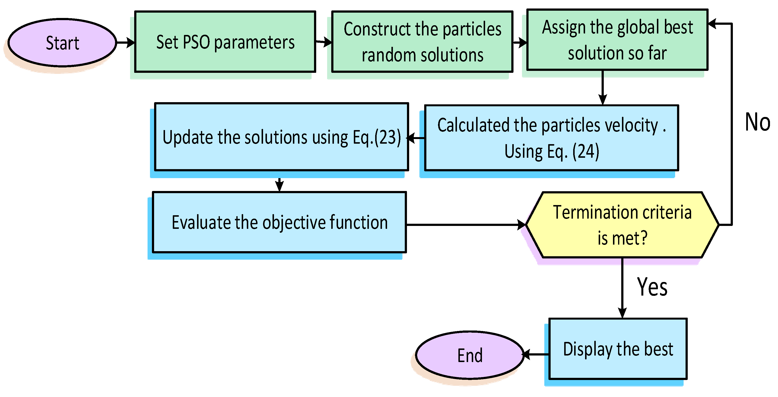
3.3. The Proposed IMPAPSO Structure

The profile that the agents follow while modifying their positions is one of the essential factors that reflect the algorithm response. Therefore, in this work two strategies are applied to enhance the MPA behavior, where the random walk of the predictor is boosted by the high-tailed Weibull distribution and its exploitation phase is strengthened by the PSO operator, as described in the following points and described in Algorithm 1.
In the first modification, the random walk of the agents in MPA that is controlled by Brownian movement to modify the predator movement is replaced by the high-tailed Weibull distribution (WD) [68], to boost the exploration stage, based on the following formula:
W D ( U ) = e x p ( u v   ) ζ
where v and ζ are the scale and shape parameters. In the current work, the tuned values of v and ζ are 2 and 1, respectively.
In the second modification, the PSO operator is utilized to enhance the exploitation phase of the basic MPA as a trial, to enhance the convergence behavior of the algorithm. In phase 3 of the MPA, the agents can follow MPA or PSO operators, based on a probability value, as explained below:
X i = { O p e r a t o r   o f   M P A                     p r o b i < r a n d i O p e r a t o r   o f   P S O             o t h e r w i s e
where p r o b i is a generated value on basis of the fitness function p r o b i = f i t n e s s i   i = 1 N F i t n e s s i , r a n d i is a random vector drawn from uniform distribution [0, 1]. If the value of prob i < rand i , then the operators of MPA of Equation (20) will be implemented; otherwise the operator of PSO of Equations (23) and (24) is executed.
Algorithm 1: Pseudo code of the proposed IMPAPSO
1.  Determine the MPAPSO parameters; N agents, T m a x maximum number of iteration and optimization problem bounds; X m a x   , X m i n .
2.  Compute the initial random solutions using Equation (15).
3.  Set t = 1.
4.  While (t > = T m a x )
5.  Evaluate the fitness function ( f i t n e s s i ).
6.  Determine the Elite matrix (best solution obtained so far).
7.  Use Equation (25) to calculate the Weibull distribution ( W D ) .
8.  If (t < T m a x 3 )
9.  Update the agents’ positions using Equation (18).
10. If ( T m a x 3   < t   <   2   T m a x 3 .)
11. For ( I =   1 , , N / 2 ) .
12. Update the agents’ positions using Equation (19)
13. End for
14. For ( i = N / 2 , , N ) .
15. Update the agents’ positions using Equation (20).
16. End for
17. Elseif (t > 2   T m a x 3 .)
18. If prob i   < rand i
19. Update the agents’ positions using Equation (21).
20. Else
21. Update the agents’ positions using Equations (23) and (24).
22. End if
23. End if
24. Using FADs effect and Equation (22) to update current agent.
25. T = t + 1
26. End while
27. Display the best solution

4. Simulation Results

In this study, the three systems are tested, these are IEEE 30-bus, 57-bus, and 118-bus standard test networks. The main reason for choosing these systems is that, they are the most popular systems used for the ORPD problem. Moreover, the MPA quality can be tested with increasing dimension systems. The standard IEEE 30-bus system contains 5 voltage buses, 21 loads, 41 branches, 4 changers, as well as 3 shunt capacitors [68]. Regarding the IEEE 57- bus test system, it contains 6 voltage buses, 41 loads, 80 branches, 17 tap changers, and 3 shunt VAR compensators. Additionally, in the IEEE 118-bus system, there are 54 voltage buses, 99 loads, 186 branches, 9 tap changers, and 14 shunt VAR compensators. The proposed IMPAPSO is inspected when applied to the aforementioned test systems for solving the ORPD Problem. Each system is studied from two points of view. These are named—‘case 1’ and ‘case 2’. Case 1, meanwhile, decreases the active power losses, and case 2 aims to reduce the deviation in voltage. To put constraints into their limits, penalty functions are inserted with constants of high value to the objective function.

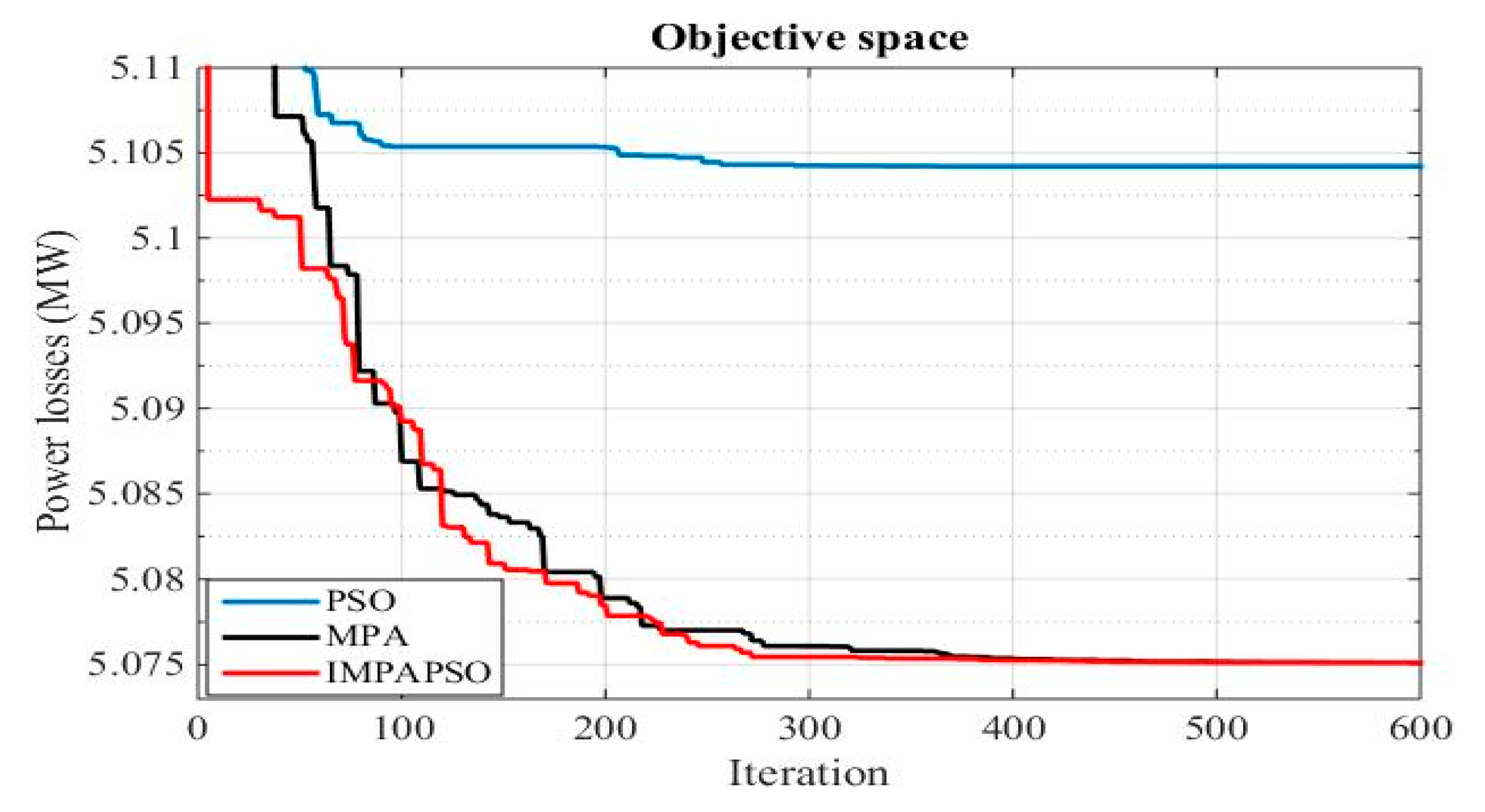
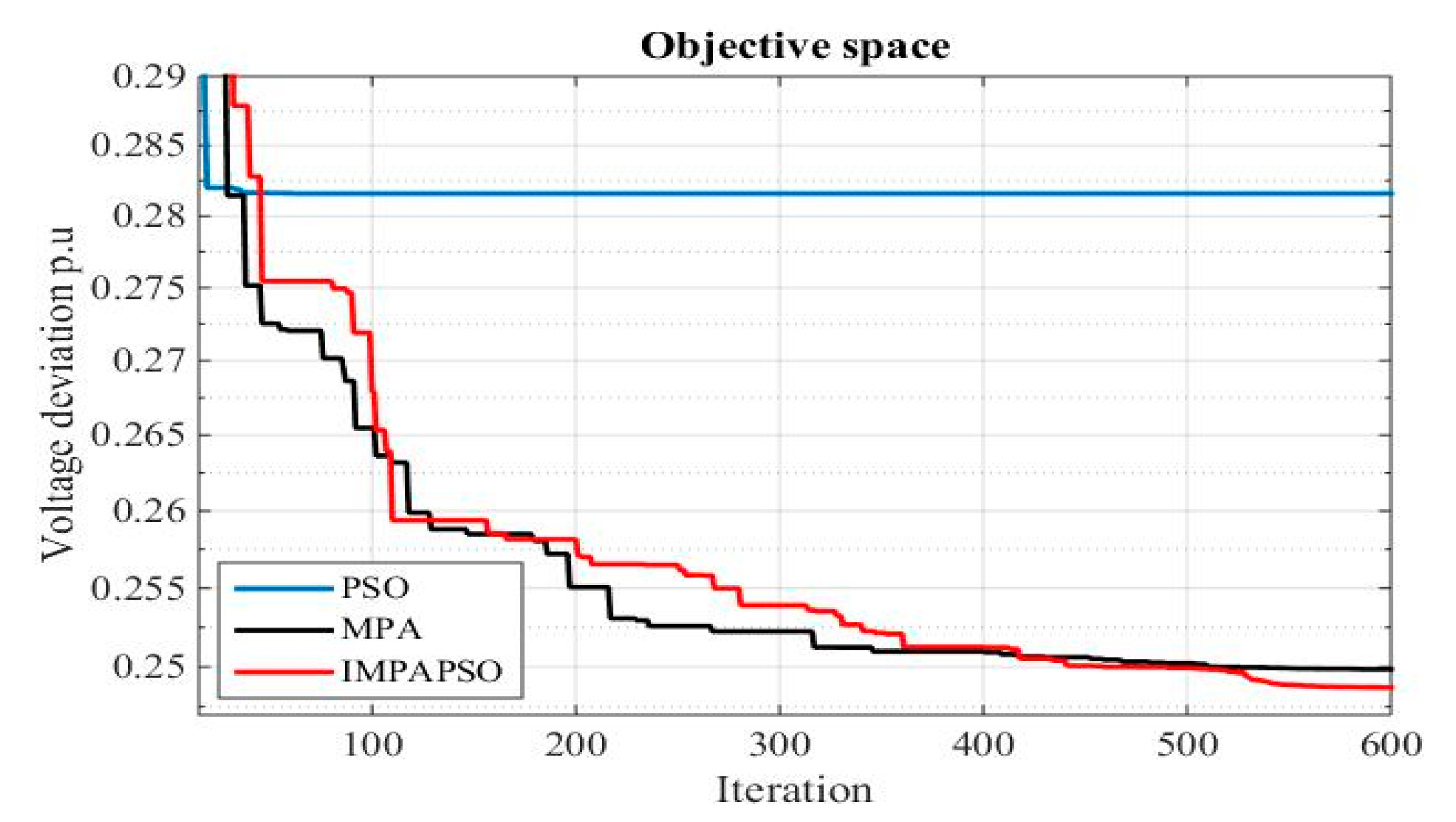
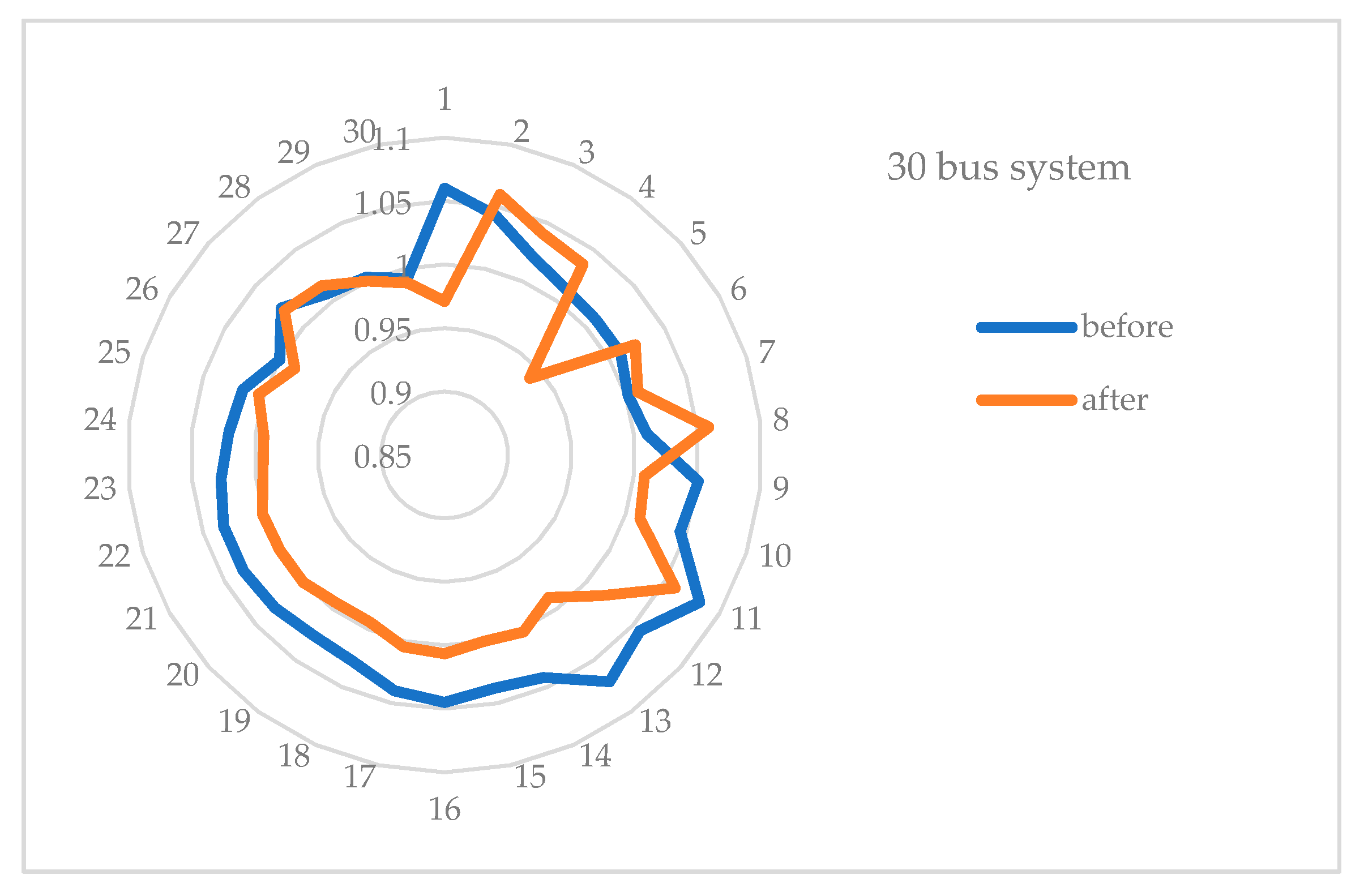
4.1. Results of the IEEE 30-Bus System

The system data are stated in [35,67]. In this network, nineteen control variables are considered. These can be stated as follows—the voltage of the generator at buses 1, 2, 5, 8, 11, and 13, transformer tap settings between the buses 6–9, 6–10, 4–12, and 28–27, in addition to the reactive power of the VAR compensators at buses 10, 12, 15, 17, 20, 21, 23, 24, and 29. The maximum and minimum values of the voltages are 1.06 and 0.94 p.u., respectively. The maximum and minimum limits of the transformer taps are 1.1 and 0.9, respectively. The minimum limit of the VAR compensators is 0 while the maximum limits are—6, 20, 6, 7, 6, 10, 6, 10, and 6 MVARs respectively. In Table 1, the results of the objective targeted in case 1 are presented in comparison with the other methods’ results. Moreover, Table 2 represents the results of the tuned decision parameters in case one, when handled by the proposed IMPAPSO. The results of these variables are compared with the results of other methods such as the HHO [66] as well as the PSO.
In the second case, the IMPAPSO is compared with other optimization methods, it reaches the minimum voltage deviation. Numerical results confirming this superiority are presented in Table 3 and Table 4. To affirm that the IMPAPSO is dependable on solving the ORPD problem, many trials are done for the two objectives under study. The convergence curves of the objective functions handled by the proposed IMPAPSO versus PSO and MPA for both the first and the second cases during 600 iterations are shown in Figure 3 and Figure 4. It could be observed that, the solution convergence of the objective functions was efficient and competitive. The values of the two objectives optimized by the IMPAPSO were the best among the methods compared.
The results of power losses in the 30 bus system obtained by different optimization methods are presented in bar chart, as shown in Figure 5. A comparison of these results showed that the value of power losses obtained by the proposed IMPAPSO optimization algorithm was the best among the results obtained by the other algorithms, especially the BFOA.
The value of the voltage at every bus in the 30-bus system is shown in Figure 6. A comparison was carried out between the bus voltage, before and after performing the ORPD problem, using the proposed IMPAPSO optimization algorithm. It was clear that the voltage profiles improved and came closer to 1 p.u., after using the IMPAPSO in the simulation process.

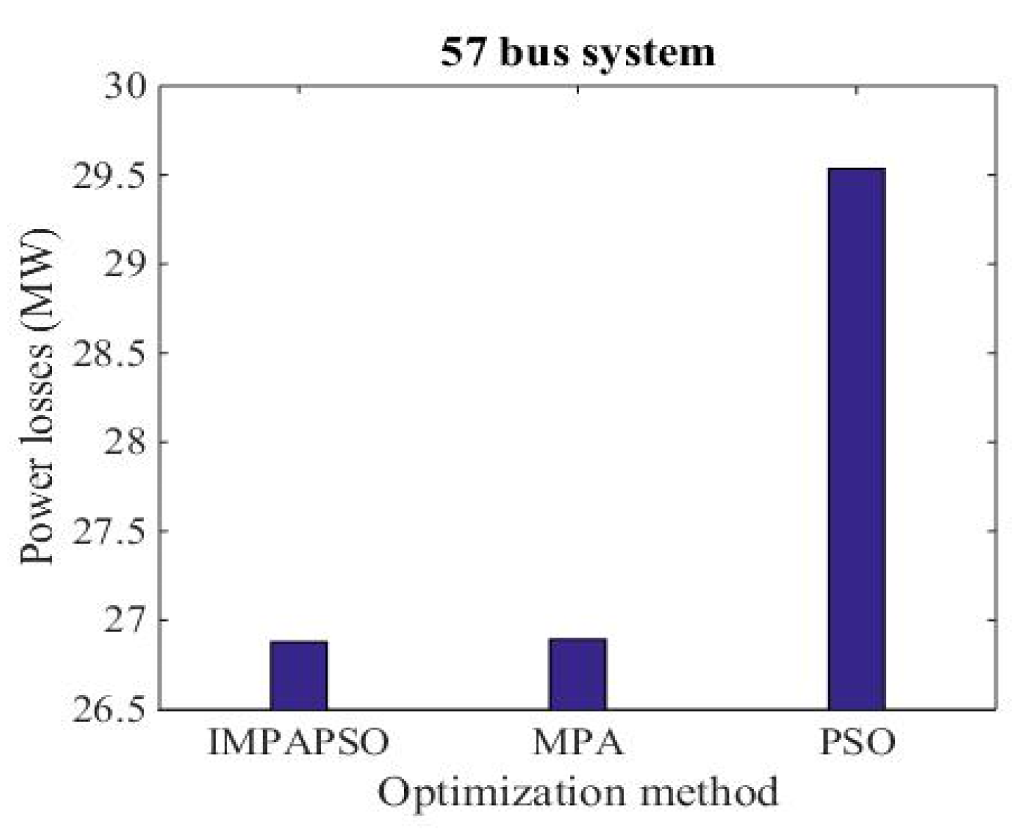
4.2. Results of the IEEE 57-Bus System

In this network, the number of control variables was 27. These could be stated as follows: generators’ voltages at buses 1, 2, 3, 6, 8, 9, and 12, transformers between the buses 4–18, 7–29, 9–55, 10–51, 11–43, 11–41, 13–49, 14–46, 15–45, 21–20, 24–26, 24–25, 34–32, 39–57, and 40–56, in addition to the reactive power of the shunt compensators at buses 18, 25, and 53. The maximum and minimum values of the voltages were 1.06 and 0.94 p.u., respectively. The maximum and minimum limits of the transformer taps were 1.1 and 0.9, respectively. The limits of the VAR compensators varied between –20 and 20 MVARs. Table 5 displays the effects of the objective function in case 1, in accordance with the results of other approaches. Moreover, Table 6 represents the results of the decision parameters in case one when handled by the IMPAPSO.
In case 2, the proposed IMPAPSO was compared with other optimization methods, it reached a minimum voltage deviation. Numerical results confirming this superiority are presented in Table 7 and Table 8. To affirm that the IMPAPSO depended on solving the ORPD problem, many trials were done for the two objectives under study. The convergence curves of the objective functions handled by the proposed IMPAPSO, MPA, and PSO for both the first and the second cases during 600 iterations are shown in Figure 7 and Figure 8. The convergence of the objective functions solutions was competitive. The values of the two objectives optimized by the IMPAPSO were the best, compared to the MPA and PSO methods.
The results of power losses in the 57 bus system obtained by different optimization methods are presented in the bar chart, as shown in Figure 9. A comparison of these results showed that the value of power losses obtained by the proposed IMPAPSO optimization algorithm was the best among the results obtained by other algorithms especially, the PSO.
Similarly, as provided in the 30 bus system, the value of the voltage at every bus in the 57 bus system is shown in Figure 10. The bus voltages were compared, before and after performing the ORPD problem, using the proposed IMPAPSO optimization algorithm. It could be noticed that the voltage values improved and came closer to 1 p.u., after using the IMPAPSO in the simulation process.

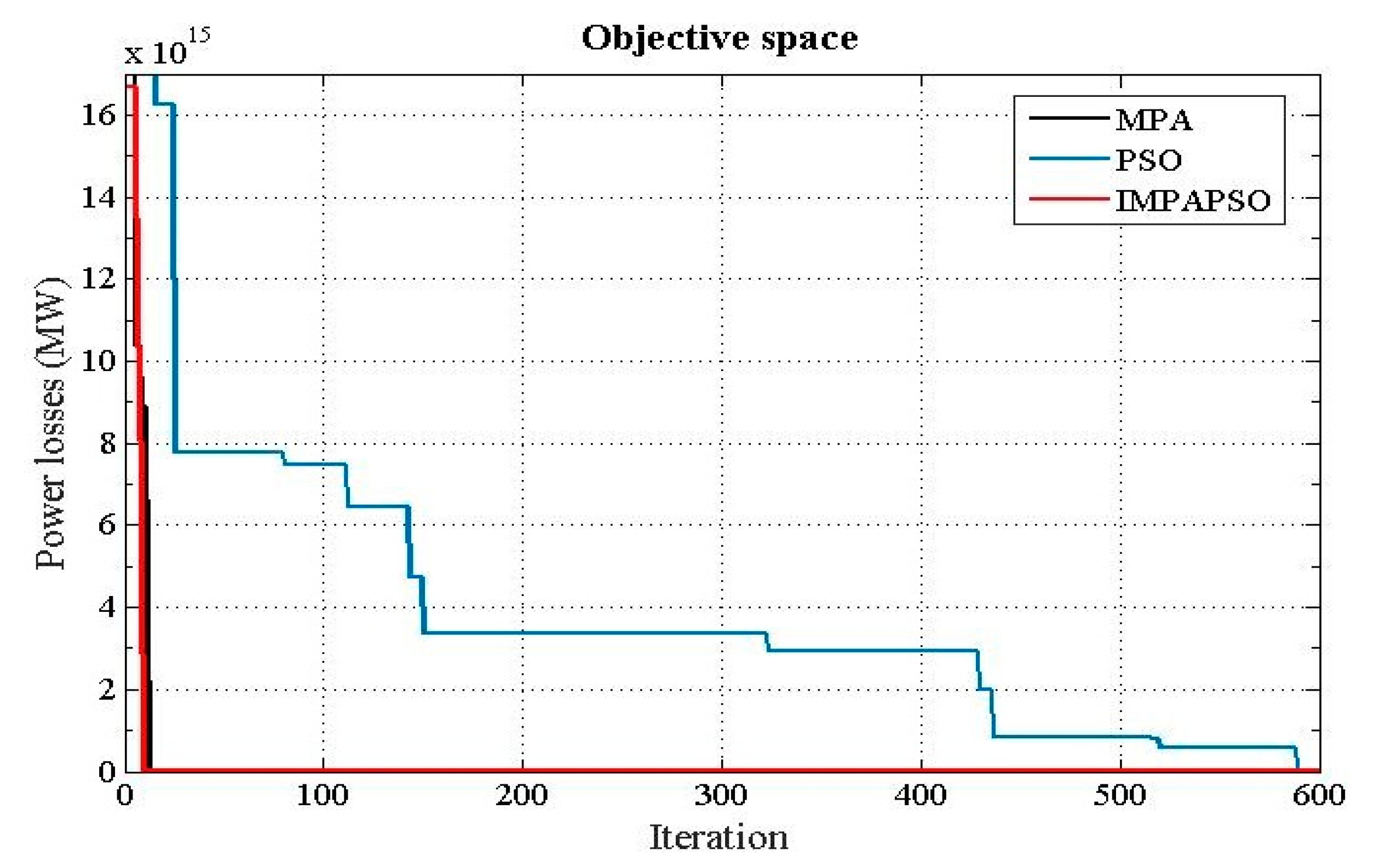
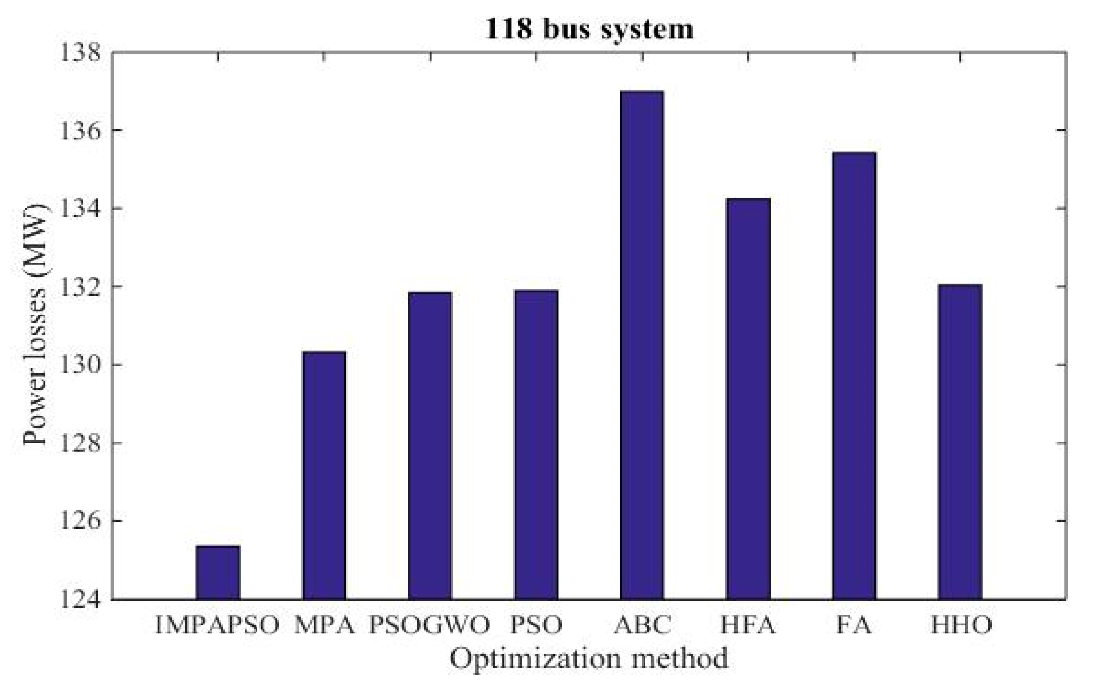
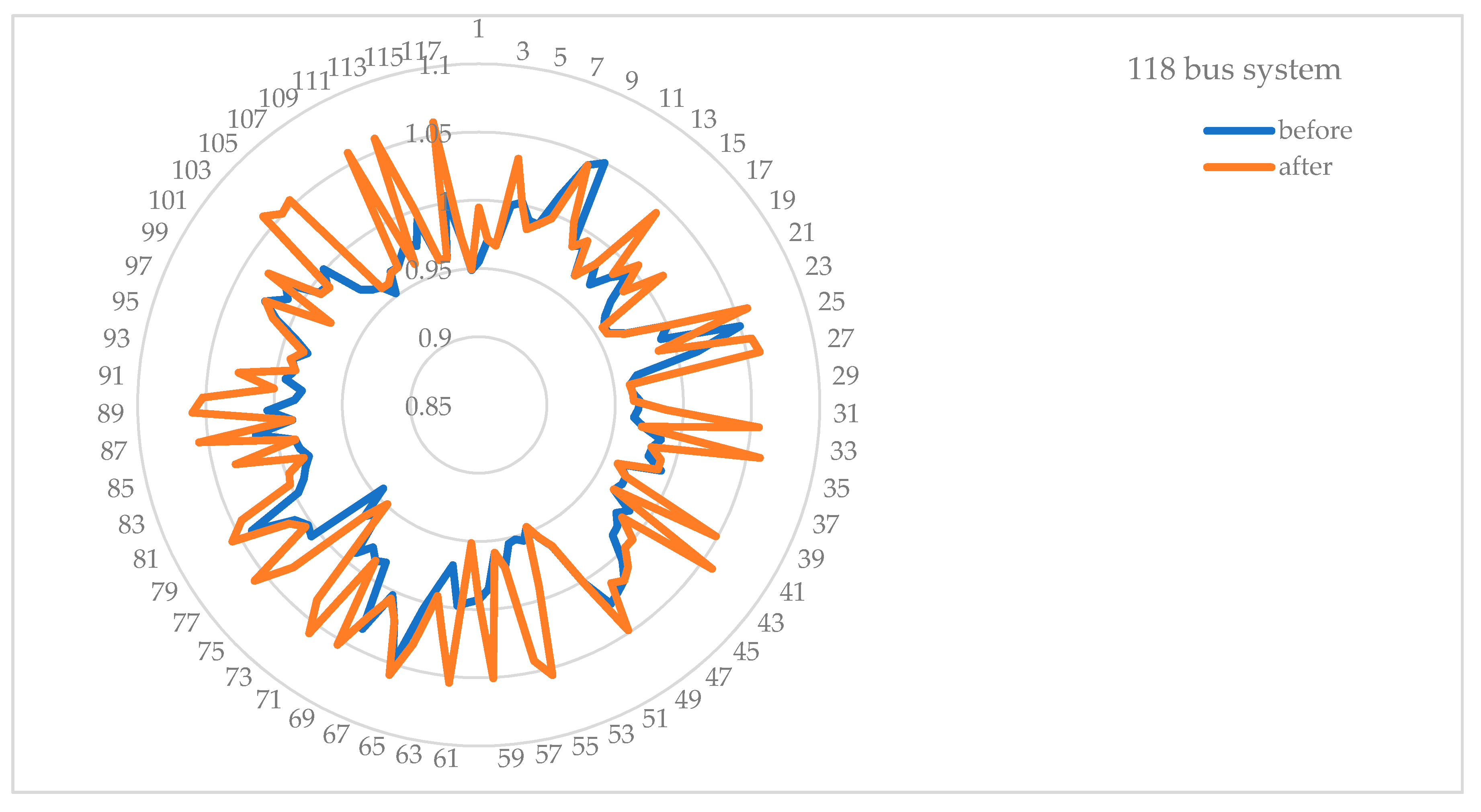
4.3. Results of the IEEE 118-Bus System

The system data are stated in [35], the number of control variables considered in this system was seventy-seven. The maximum and minimum values of the voltages were 1.06 and 0.94 p.u., respectively. The maximum and minimum limits of the transformer taps were 1.1 and 0.9, respectively. The limits of the VAR compensators varied between −20 and 20 MVARs. In Table 9, the results of the objective function in case 1 are presented in comparison with the other methods’ results. Moreover, Table 10 represents the results of the adjusted control variables in case 1 when handled by the IMPAPSO. The findings are compared with the results of other approaches, including FA, ABC, and PSO. In case 2, the IMPAPSO was compared with other optimization methods, where it reached a minimum voltage deviation. Numerical results confirming this superiority are presented in Table 11 and Table 12. To affirm that the IMPAPSO was dependent on solving the ORPD problem, many trials were done for the two objectives under study. The convergence curves in case 1 and case 2 of the objective functions handled by the proposed IMPAPSO, MPA, and PSO are shown in Figure 11 and Figure 12. It could be observed that, the convergence of the solution of the objective functions was efficient and competitive. The values of the two objectives optimized by the IMPAPSO were the best among the methods compared.
The results of power losses in the 118 bus system obtained by different optimization methods are presented in the bar chart, as shown Figure 13. A comparison of these results showed that the value of power losses obtained by the IMPAPSO algorithm was the best among the results obtained by other algorithms, especially the ABC and the FA.
The voltage at every bus in the 118-bus system is shown in Figure 14. The bus voltages were compared before and after performing the ORPD problem, using the IMPAPSO algorithm. Notably, the voltage values were improved after using the IMPAPSO in the simulation.

5. Conclusions

The paper presented a new application of the IMPAPSO to solve the ORPD problem. The objective functions were also mathematically formulated and introduced. The optimization technique was inspected with 30, 57, and 118 bus test systems. The review observed that, it was mostly studied to minimize real power losses in power systems, especially in transmission networks for the ORPD problem. Therefore, in this article, two case studies were evaluated where the ORPD problem was solved by IMPAPSO, MPA, and PSO. Two points of view optimized the objective functions of the problem. First, the active power losses must be minimized. In addition, the second goal was to minimize the deviation in voltage. The performance of IMPAPSO was compared with other well-known methods incorporated optimizers. The tool in this paper, as shown by the simulation results, was able to find improved solutions to the ORPD problem. The advantages and superiority were investigated on various test systems. The employment of the proposed method resulted in an improvement in power loss minimization up to 96% in the 30-bus system, 10% in the 57-bus system, and 9% in the 118-bus system. Additionally, the improvement in voltage deviation minimization due to the usage of IMPAPSO was up to 18% in the 30-bus system, 33% in the 57-bus system, and 12% in the 118-bus system. Furthermore, the results of the simulation confirmed that, the IMPAPSO could be applied to additional electricity grid problems. Last, the results obtained by other optimization algorithms were statistically presented to compare the performance of the discussed algorithms. It is expected that the proposed IMPAPSO would be a magnet for the researchers who are interested in optimization of different power engineering problems.

Author Contributions

H.M.H.: Formal analysis, Investigation of the results and the proposed algorithm, Methodology suggestion, Supervisor of the team, Validation to the results, review & editing the article; A.A.: Funding acquisition, financial support through the reseach project stated in the acknowledgement, Simulation, review; D.Y.: Methodology suggestion, Software modification to get enhanced results, Writing and editing the section of the proposed algorithm, reviewing the introduction part; A.F.: Investigation of the results, review and editing; S.M.M.: review and editing. Eng. M.A.M.S.: Software modification, Simulation, writing, and editing. All authors have read and agreed to the published version of the manuscript.

Funding

This research was funded by Researchers Supporting Project number (RSP-2020/258), King Saud University, Riyadh, Saudi Arabia.

Acknowledgments

The authors would like to thank Researchers Supporting Project number (RSP-2020/258), King Saud University, Riyadh, Saudi Arabia.

Conflicts of Interest

The authors declare no conflict of interest.

References

  1. Vlachogiannis, J.G.; Lee, K.Y. Quantum-Inspired Evolutionary Algorithm for Real and Reactive Power Dispatch. IEEE Trans. Power Syst. 2008, 23, 1627–1636. [Google Scholar] [CrossRef] [Green Version]
  2. Dommel, H.W.; Tinney, W.F. Optimal Power Flow Solutions. IEEE Trans. Power Appar. Syst. 1968, 10, 1866–1876. [Google Scholar] [CrossRef]
  3. Robbins, B.A.; Dominguez-Garcia, A.D. Optimal Reactive Power Dispatch for Voltage Regulation in Unbalanced Distribution Systems. IEEE Trans. Power Syst. 2016, 31, 2903–2913. [Google Scholar] [CrossRef]
  4. Shaheen, A.M.; Farrag, S.M.; El-Sehiemy, R.A. MOPF solution methodology. IET Gener. Transm. Distrib. 2017, 11, 570–581. [Google Scholar] [CrossRef]
  5. Sakr, W.S.; El-Sehiemy, R.A.; Azmy, A.M. Adaptive differential evolution algorithm for efficient reactive power management. Appl. Soft Comput. 2017, 53, 336–351. [Google Scholar] [CrossRef]
  6. Singh, H.; Srivastava, L. Modified Differential Evolution algorithm for multi-objective VAR management. Int. J. Electr. Power Energy Syst. 2014, 55, 731–740. [Google Scholar] [CrossRef]
  7. Mehdinejad, M.; Mohammadi-Ivatloo, B.; Dadashzadeh-Bonab, R.; Zare, K. Solution of optimal reactive power dispatch of power systems using hybrid particle swarm optimization and imperialist competitive algorithms. Int. J. Electr. Power Energy Syst. 2016, 83, 104–116. [Google Scholar] [CrossRef]
  8. Saddique, M.S.; Bhatti, A.R.; Haroon, S.S.; Sattar, M.K.; Amin, S.; Sajjad, I.A.; Haq, S.S.U.; Awan, A.B.; Rasheed, N. Solution to optimal reactive power dispatch in transmission system using meta-heuristic techniques―Status and technological review. Electr. Power Syst. Res. 2020, 178, 106031. [Google Scholar] [CrossRef]
  9. Polprasert, J.; Ongsakul, W.; Vo, D.N. Optimal Reactive Power Dispatch Using Improved Pseudo-gradient Search Particle Swarm Optimization. Electr. Power Compon. Syst. 2016, 44, 518–532. [Google Scholar] [CrossRef]
  10. Lee, K.; Yang, F. Optimal reactive power planning using evolutionary algorithms: A comparative study for evolutionary programming, evolutionary strategy, genetic algorithm, and linear programming. IEEE Trans. Power Syst. 1998, 13, 101–108. [Google Scholar] [CrossRef]
  11. Zhu, J.; Xiong, X. Optimal reactive power control using modified interior point method. Electr. Power Syst. Res. 2003, 66, 187–192. [Google Scholar] [CrossRef]
  12. Quintana, V.H.; Santos-Nieto, M. Reactive-power dispatch by successive quadratic programming. IEEE Trans. Energy Convers. 1989, 4, 425–435. [Google Scholar] [CrossRef]
  13. Jan, R.-M.; Chen, N. Application of the fast Newton-Raphson economic dispatch and reactive power/voltage dispatch by sensitivity factors to optimal power flow. IEEE Trans. Energy Convers. 1995, 10, 293–301. [Google Scholar] [CrossRef]
  14. Wu, Q.; Cao, Y.; Wen, J. Optimal reactive power dispatch using an adaptive genetic algorithm. Int. J. Electr. Power Energy Syst. 1998, 20, 563–569. [Google Scholar] [CrossRef]
  15. El-Ela, A.A.A.; Kinawy, A.M.; El Sehiemy, R.A.; Mouwafi, M.T. Optimal reactive power dispatch using ant colony optimization algorithm. Electr. Eng. 2011, 93, 103–116. [Google Scholar] [CrossRef]
  16. Shaheen, M.A.M.; Hasanien, H.M.; Mekhamer, S.F.; Talaat, H.E.A. Optimal Power Flow of Power Systems Including Distributed Generation Units Using Sunflower Optimization Algorithm. IEEE Access 2019, 7, 109289–109300. [Google Scholar] [CrossRef]
  17. Qais, M.H.; Alghuwainem, S.; Alghuwainem, S. Identification of electrical parameters for three-diode photovoltaic model using analytical and sunflower optimization algorithm. Appl. Energy 2019, 250, 109–117. [Google Scholar] [CrossRef]
  18. Shaheen, M.A.M.; Mekhamer, S.F.; Hasanien, H.M.; Talaat, H.E.A. Optimal Power Flow of Power Systems Using Hybrid Firefly and Particle Swarm Optimization Technique. In Proceedings of the 2019 21st International Middle East Power Systems Conference (MEPCON), Cairo, Egypt, 17–19 December 2019; pp. 232–237. [Google Scholar]
  19. Duman, S.; Sonmez, Y.; Guvenc, U.; Yorukeren, N. Optimal reactive power dispatch using a gravitational search algorithm. IET Gener. Transm. Distrib. 2012, 6, 563. [Google Scholar] [CrossRef]
  20. Lenin, K.; Reddy, B.R.; Kalavathi, M.S. Brainstorm optimization algorithm for solving optimal reactive power dispatch problem. Int. J. Res. Electron. Commun. Technol. 2014, 1, 25–30. [Google Scholar]
  21. El-Fergany, A.A.; Hasanien, H.M. Tree-seed algorithm for solving optimal power flow problem in large-scale power systems incorporating validations and comparisons. Appl. Soft Comput. 2017, 64, 307–316. [Google Scholar] [CrossRef]
  22. El-Fergany, A.A.; Hasanien, H.M. Salp swarm optimizer to solve optimal power flow comprising voltage stability analysis. Neural Comput. Appl. 2019, 32, 5267–5283. [Google Scholar] [CrossRef]
  23. Hasanien, H.M.; El-Fergany, A.A. Salp swarm algorithm-based optimal load frequency control of hybrid renewable power systems with communication delay and excitation cross-coupling effect. Electr. Power Syst. Res. 2019, 176, 0378–7796. [Google Scholar] [CrossRef]
  24. Qais, M.H.; Alghuwainem, S.; Alghuwainem, S. Enhanced salp swarm algorithm: Application to variable speed wind generators. Eng. Appl. Artif. Intell. 2019, 80, 82–96. [Google Scholar] [CrossRef]
  25. Attia, A.-F.; El-Sehiemy, R.A.; Hasanien, H.M. Optimal power flow solution in power systems using a novel Sine-Cosine algorithm. Int. J. Electr. Power Energy Syst. 2018, 99, 331–343. [Google Scholar] [CrossRef]
  26. Qais, M.H.; Hasanien, H.M.; Alghuwainem, S.; Nouh, A.S. Coyote optimization algorithm for parameters extraction of three-diode photovoltaic models of photovoltaic modules. Energy 2019, 187, 15. [Google Scholar] [CrossRef]
  27. Dai, C.; Chen, W.; Zhu, Y.; Zhang, X. Seeker Optimization Algorithm for Optimal Reactive Power Dispatch. IEEE Trans. Power Syst. 2009, 24, 1218–1231. [Google Scholar] [CrossRef]
  28. Amjady, N.; Fatemi, H.; Zareipour, H. Solution of Optimal Power Flow Subject to Security Constraints by a New Improved Bacterial Foraging Method. IEEE Trans. Power Syst. 2012, 27, 1311–1323. [Google Scholar] [CrossRef]
  29. Yousri, D.; Mirjalili, S. Fractional-order cuckoo search algorithm for parameter identification of the fractional-order chaotic, chaotic with noise and hyper-chaotic financial systems. Eng. Appl. Artif. Intell. 2020, 92, 103662. [Google Scholar] [CrossRef]
  30. Mujtaba, M.; Masjuki, H.; Kalam, M.; Ong, H.C.; Gul, M.; Farooq, M.; Soudagar, M.E.M.; Ahmed, W.; Harith, M.; Yusoff, M. Ultrasound-assisted process optimization and tribological characteristics of biodiesel from palm-sesame oil via response surface methodology and extreme learning machine—Cuckoo search. Renew. Energy 2020, 158, 202–214. [Google Scholar] [CrossRef]
  31. Kalaam, R.N.; Muyeen, S.; Al-Durra, A.; Hasanien, H.M.; Al-Wahedi, K. Optimisation of controller parameters for grid-tied photovoltaic system at faulty network using artificial neural network-based cuckoo search algorithm. IET Renew. Power Gener. 2017, 11, 1517–1526. [Google Scholar] [CrossRef]
  32. ElAzab, O.S.; Alghuwainem, S.; Alsaidan, I.; Abdelaziz, A.Y.; Khalid, H.M. Parameter Estimation of Three Diode Photovoltaic Model Using Grasshopper Optimization Algorithm. Energies 2020, 13, 497. [Google Scholar] [CrossRef] [Green Version]
  33. Qais, M.H.; Hasanien, H.M.; Alghuwainem, S. Parameters extraction of three-diode photovoltaic model using computation and Harris Hawks optimization. Energy 2020, 195, 117040. [Google Scholar] [CrossRef]
  34. Li, Y.; Wang, Y.; Li, B. A hybrid artificial bee colony assisted differential evolution algorithm for optimal reactive power flow. Int. J. Electr. Power Energy Syst. 2013, 52, 25–33. [Google Scholar] [CrossRef]
  35. Shaheen, M.A.; Hasanien, H.M.; Alkuhayli, A. A novel hybrid GWO-PSO optimization technique for optimal reactive power dispatch problem solution. Ain Shams Eng. J. 2020. [Google Scholar] [CrossRef]
  36. Gafar, M.G.; El Sehiemy, R.A.; Hasanien, H.M. A Novel Hybrid Fuzzy-JAYA Optimization Algorithm for Efficient ORPD Solution. IEEE Access 2019, 7, 182078–182088. [Google Scholar] [CrossRef]
  37. Liang, R.-H.; Wang, J.-C.; Chen, Y.-T.; Tseng, W.-T. An enhanced firefly algorithm to multi-objective optimal active/reactive power dispatch with uncertainties consideration. Int. J. Electr. Power Energy Syst. 2015, 64, 1088–1097. [Google Scholar] [CrossRef]
  38. Devaraj, D.; Roselyn, J.P. Genetic algorithm based reactive power dispatch for voltage stability improvement. Int. J. Electr. Power Energy Syst. 2010, 32, 1151–1156. [Google Scholar] [CrossRef]
  39. Hasanien, H.M. Particle Swarm Design Optimization of Transverse Flux Linear Motor for Weight Reduction and Improvement of Thrust Force. IEEE Trans. Ind. Electron. 2011, 58, 4048–4056. [Google Scholar] [CrossRef]
  40. Badar, A.Q.; Umre, B.; Junghare, A. Reactive power control using dynamic Particle Swarm Optimization for real power loss minimization. Int. J. Electr. Power Energy Syst. 2012, 41, 133–136. [Google Scholar] [CrossRef]
  41. Zhihuan, L.; Yinhong, L.; Xianzhong, D. Non-dominated sorting genetic algorithm-II for robust multi-objective optimal reactive power dispatch. IET Gener. Transm. Distrib. 2010, 4, 1000. [Google Scholar] [CrossRef]
  42. Biswas, P. Genetic Algorithm Based Multiobjective Bilevel Programming for Optimal Real and Reactive Power Dispatch Under Uncertainty. In Computational Intelligence Applications in Modeling and Control; Springer: Berlin/Heidelberg, Germany, 2015; pp. 171–203. [Google Scholar]
  43. Varadarajan, M.; Swarup, K. Differential evolutionary algorithm for optimal reactive power dispatch. Int. J. Electr. Power Energy Syst. 2008, 30, 435–441. [Google Scholar] [CrossRef]
  44. Orosz, T.; Rassõlkin, A.; Kallaste, A.; Arsénio, P.; Pánek, D.; Kaska, J.; Karban, P. Robust Design Optimization and Emerging Technologies for Electrical Machines: Challenges and Open Problems. Appl. Sci. 2020, 10, 6653. [Google Scholar] [CrossRef]
  45. Ghasemi, M.; Ghavidel, S.; Ghanbarian, M.M.; Habibi, A. A new hybrid algorithm for optimal reactive power dispatch problem with discrete and continuous control variables. Appl. Soft Comput. 2014, 22, 126–140. [Google Scholar] [CrossRef]
  46. Das, D.B.; Patvardhan, C. Reactive power dispatch with a hybrid stochastic search technique. Int. J. Electr. Power Energy Syst. 2002, 24, 731–736. [Google Scholar] [CrossRef]
  47. Das, D.B.; Patvardhan, C. A new hybrid evolutionary strategy for reactive power dispatch. Electr. Power Syst. Res. 2003, 65, 83–90. [Google Scholar] [CrossRef]
  48. Yan, W.; Lu, S.; Yu, D. A Novel Optimal Reactive Power Dispatch Method Based on an Improved Hybrid Evolutionary Programming Technique. IEEE Trans. Power Syst. 2004, 19, 913–918. [Google Scholar] [CrossRef]
  49. Chung, C.; Liang, C.; Wong, K.; Duan, X. Hybrid algorithm of differential evolution and evolutionary programming for optimal reactive power flow. IET Gener. Transm. Distrib. 2010, 4, 84. [Google Scholar] [CrossRef]
  50. Abdel-Fatah, S.; Ebeed, M.; Kamel, S. Optimal reactive power dispatch using modified sine cosine algorithm. In Proceedings of the 2019 International Conference on Innovative Trends in Computer Engineering (ITCE), Aswan, Egypt, 2–4 February 2019; pp. 510–514. [Google Scholar]
  51. Yan, W.; Liu, F.; Chung, C.; Wong, K. A Hybrid Genetic Algorithm–Interior Point Method for Optimal Reactive Power Flow. IEEE Trans. Power Syst. 2006, 21, 1163–1169. [Google Scholar] [CrossRef] [Green Version]
  52. Ghasemi, M.; Ghanbarian, M.M.; Ghavidel, S.; Rahmani, S.; Moghaddam, E.M. Modified teaching learning algorithm and double differential evolution algorithm for optimal reactive power dispatch problem: A comparative study. Inf. Sci. 2014, 278, 231–249. [Google Scholar] [CrossRef]
  53. Nguyen, T.T.; Vo Ngoc, D. Improved social spider optimization algorithm for optimal reactive power dispatch problem with different objectives. Neural Comput. Appl. 2019, 32, 5919–5950. [Google Scholar] [CrossRef]
  54. Srivastava, L.; Singh, H. Hybrid multi-swarm particle swarm optimisation based multi-objective reactive power dispatch. IET Gener. Transm. Distrib. 2015, 9, 727–739. [Google Scholar] [CrossRef]
  55. Rajan, A.; Malakar, T. Optimal reactive power dispatch using hybrid Nelder–Mead simplex based firefly algorithm. Int. J. Electr. Power Energy Syst. 2015, 66, 9–24. [Google Scholar] [CrossRef]
  56. Prasad, D.; Banerjee, A.; Singh, R.P. Optimal reactive power dispatch using modified differential evolution algorithm. In Advances in Computer, Communication and Control; Springer: Singapore, 2019; pp. 275–283. [Google Scholar]
  57. Jeyadevi, S.; Baskar, S.; Babulal, C.; Iruthayarajan, M.W. Solving multiobjective optimal reactive power dispatch using modified NSGA-II. Int. J. Electr. Power Energy Syst. 2011, 33, 219–228. [Google Scholar] [CrossRef]
  58. Faramarzi, A.; Heidarinejad, M.; Mirjalili, S.; Gandomi, A.H. Marine Predators Algorithm: A nature-inspired metaheuristic. Expert Syst. Appl. 2020, 152, 113377. [Google Scholar] [CrossRef]
  59. Yousri, D.; Babu, T.S.; Beshr, E.; Eteiba, M.B.; Allam, D. A Robust Strategy Based on Marine Predators Algorithm for Large Scale Photovoltaic Array Reconfiguration to Mitigate the Partial Shading Effect on the Performance of PV System. IEEE Access 2020, 8, 112407–112426. [Google Scholar] [CrossRef]
  60. Yousri, D.; Elaziz, M.A.; Oliva, D.; Abualigah, L.; Al-Qaness, M.A.A.; Ewees, A.A. Reliable applied objective for identifying simple and detailed photovoltaic models using modern metaheuristics: Comparative study. Energy Convers. Manag. 2020, 223, 113279. [Google Scholar] [CrossRef]
  61. Soliman, M.A.; Hasanien, H.M.; Alkuhayli, A. Marine Predators Algorithm for Parameters Identification of Triple-Diode Photovoltaic Models. IEEE Access 2020, 8, 155832–155842. [Google Scholar] [CrossRef]
  62. Al-Qaness, M.A.A.; Ewees, A.A.; Fan, H.; Abualigah, L.; Elaziz, M.A. Marine Predators Algorithm for Forecasting Confirmed Cases of COVID-19 in Italy, USA, Iran and Korea. Int. J. Environ. Res. Public Health 2020, 17, 3520. [Google Scholar] [CrossRef]
  63. Russell, E.; Kennedy, J. “A new optimizer using particle swarm theory” MHS’95. In Proceedings of the Sixth International Symposium on Micro Machine and Human Science, Nagoya, Japan, 4–6 October 1995. [Google Scholar]
  64. El Sehiemy, R.A.; El Ela, A.A.A.; Shaheen, A. A Multi-Objective Fuzzy-Based Procedure for Reactive Power-Based Preventive Emergency Strategy. Int. J. Eng. Res. Afr. 2014, 13, 91–102. [Google Scholar] [CrossRef]
  65. Bhattacharya, A.; Chattopadhaya, P.K. Solution of optimal reactive power flow using biogeography-based optimization. Int. J. Electr. Electron. Eng. 2010, 4, 568–576. [Google Scholar]
  66. Omid, K. Generalized weighted Weibull distribution. J. Math. Ext. 2016, 10, 89–118. [Google Scholar]
  67. Qasem, S.N.; Shamsuddin, S.M.; Hassanien, A.E. Hybrid learning enhancement of RBF network with particle swarm optimization. In Foundations of Computational, Intelligence Volume 1; Springer: Berlin/Heidelberg, Germany, 2009; pp. 381–397. [Google Scholar]
  68. Matpower. Available online: https://matpower.org/ (accessed on 20 March 2018).
Figure 1. Flow diagram of the marine predators algorithm (MPA).
Energies 13 05679 g001
Figure 2. Flow diagram of the Particle Swarm Optimizer (PSO) algorithm.
Energies 13 05679 g002
Figure 3. Convergence of PSO, MPA, and IMPAPSO in the first case of the IEEE 30-bus system.
Energies 13 05679 g003
Figure 4. Convergence of PSO, MPA, and IMPAPSO in the second case of the IEEE 30-bus system.
Energies 13 05679 g004
Figure 5. Power losses obtained by different optimization methods for 30 bus system.
Energies 13 05679 g005
Figure 6. Bus voltages of the 30-bus system before and after ORPD.
Energies 13 05679 g006
Figure 7. Convergence of PSO, MPA, and IMPAPSO in the first case of the IEEE 57-bus system.
Energies 13 05679 g007
Figure 8. Convergence of PSO, MPA, and IMPAPSO in the second case of the IEEE 57-bus system.
Energies 13 05679 g008
Figure 9. Power losses obtained by different optimization methods for the 57 bus system.
Energies 13 05679 g009
Figure 10. Bus voltages of 57 bus system before and after optimal reactive power dispatch (ORPD).
Energies 13 05679 g010
Figure 11. Convergence of PSO, MPA, and IMPAPSO in the first case of the IEEE 118-bus system.
Energies 13 05679 g011
Figure 12. Convergence of PSO and IMPAPSO in the second case of the IEEE 118-bus system.
Energies 13 05679 g012
Figure 13. Power losses obtained by different optimization methods for 118 bus system.
Energies 13 05679 g013
Figure 14. Bus voltages of 118 bus system before and after ORPD.
Energies 13 05679 g014
Table 1. IEEE 30-bus system’s first case objective performance.
Optimization TechniqueIMPAPSOMPAPSOGWO [35]PSO [35]GA [35]HHO [35]SFO [35]FA [36]ABC [36]BFOA [36]
Ploss (MW)5.075109415.075120465.0903705.14405.09805.14405.10705.605.79010.010
Table 2. 30-bus system decision variables for the first case.
Control VariablesVoltage at Bus 10.969730674
21.059513441
50.973780336
81.038276148
110.989374409
131.04492558
Shunt Capacitor at Bus 100.000849981
120.022132174
154.360122795
174.605427221
203.555960479
218.766802937
231.669302394
242.780276654
292.071843038
Transformer Setting at Branch 110.975423173
121.038573785
150.967390297
360.942683073
Table 3. IEEE 30-bus system’s second case objective performance.
Optimization TechniqueIMPAPSOMPAPSOGWO [35]PSO [35]GA [35]SFO [36]GSA [36]
VD (p.u)0.2487072983750.2498495310.27800.281600.455300.398300.46720
Table 4. 30-bus system decision variables for the second case.
Control VariablesVoltage at Bus 10.971114325
21.059773514
50.940273757
81.059266477
111.059803329
130.989082988
Shunt Capacitor at Bus 100.008843572
120.032670671
150.073551739
170.001407284
203.972302965
210.03376219
230.337955988
240.005442228
290.016140404
Transformer Setting at Branch 111.099993675
120.977432649
151.08684784
360.962519663
Table 5. IEEE 57-bus system’s first case objective performance.
Optimization TechniqueIMPAPSOMPAPSO [35]
Ploss (MW)26.878828016327626.8927602429.535
Table 6. 57-bus system decision variables for the first case.
Control VariablesVoltage at Bus 10.9785146
21.052823232
30.974021524
61.011493737
81.057673755
91.018774788
121.010605445
Shunt Capacitor at Bus 182.221922839
259.245578409
537.19914277
Transformer Setting at Branch 190.958381183
200.904800844
311.006567915
350.98703182
361.023725329
371.001223982
410.928721206
460.9501672
540.900034255
580.929622764
590.917319339
650.935144142
660.90000018
710.910289969
731.004015592
760.971722216
800.921100395
Table 7. IEEE 57-bus system’s second case objective performance.
Optimization TechniqueIMPAPSOMPAPSO [35]
VD (p.u)0.681058821284250.6852172690.90660
Table 8. 57-bus system decision variables for the second case.
Control VariablesVoltage at Bus 11.051118197
21.006268088
31.055046116
61.016574856
81.039084119
90.986277586
121.053706517
Shunt Capacitor at Bus 1819.989606
2517.41486434
5319.99677651
Transformer Setting at Branch 191.036557631
201.037392917
310.972303544
351.099043364
361.08965409
371.008104923
410.984263129
460.918450377
540.900000712
580.917622635
590.959332835
650.989726479
660.900000408
710.916607993
731.016134546
760.900040954
800.9708587
Table 9. IEEE 118-bus system’s first case objective performance.
Optimization TechniqueIMPAPSOMPAPSOGWO [35]PSO [35]ABC [36]HFA [36]FA [36]HHO [35]
Ploss (MW)125.354105139297130.3235948131.84580131.89750136.990134.240135.420132.03940
Table 10. 118-bus system decision variables for the first case.
Control VariablesVoltage at Bus 11.059999971891.043844801
41.016416799901.059992049
61.06911.051300073
81.054076587920.985511829
101.059994707991.039516442
120.994109181000.949906401
151.0599949531031.012269278
181.059998621041.059986665
191.0258835951050.940166842
241.057645731071.059968135
251.0463456451101.059984578
261.059869191110.954159655
270.9656205281121.0599967
311.0007351261131.014186953
321.0583888971161.059999935
340.985688654Shunt Capacitor at Bus 53.380169875
361.05979013434-2.821486649
400.940000553379.324728941
421.058036022444.426816441
460.9400011024519.99999749
491.059922276468.73004765
541.059983552484.575662665
551.0599999447411.57140726
561.03942602779-0.964210364
591.005329927820.990696573
611.05981758383-5.073112353
621.0599999111051.021595682
650.9558352731070.999709578
661.061100.986601382
691.059395276Transformer Setting at Branch 81.016684284
701.056639777320.959359111
721.000774907361.054434837
731.058904539510.904481479
741.002748512931.082529747
760.949002597951.078129104
771.0596087331021.1
800.9400022461070.972662338
851.0595727171271.099804308
871.054263227
Table 11. IEEE 118-bus system’s second case objective performance.
Optimization TechniqueIMPAPSOMPAPSOGWO [35]HHO [35]PSO [35]
VD (p.u)1.258667409535671.26103431.266548351.359201.4090
Table 12. 118-bus system decision variables for the second case.
Control VariablesVoltage at Bus 10.994744207891.059872194
41.032754573901.052362524
60.983468712911.000606645
80.996835667921.027502208
101.000996814990.974053361
120.9940560751001.031654994
151.0414119621031.059959876
180.9846475911041.050964784
191.0149961571051.054261795
241.0591720721070.960638959
250.9877161761101.058150059
261.0557715891110.963489053
271.0594889421121.059578383
310.9875118631131.002132787
321.0558989941161.059829228
341.059602516Shunt Capacitor at Bus 515.28908452
360.98933012834-15.47848546
401.0486352683719.81999374
421.058931563445.309899212
461.011354054514.44671525
491.048205061467.474022543
540.99051842948-19.89917294
551.05524590774-19.98714174
561.0419527777919.99555592
591.050709535820.999385959
610.9514046918319.52520002
621.0547681671050.982597669
651.03115811071.002484969
661.0583800641101.01887486
691.024901644Transformer Setting at Branch 80.995503204
701.054006711320.963829517
721.058519122360.900014144
731.035636318510.947148952
740.948833087931.099941872
761.030934246950.952418082
771.0587796161020.92300055
801.0564377851070.900249471
851.0334873711271.058883247
871.056857442
Publisher’s Note: MDPI stays neutral with regard to jurisdictional claims in published maps and institutional affiliations.

