Potential Energy, Demand, Emissions, and Cost Savings Distributions for Buildings in a Utility’s Service Area


Oak Ridge National Laboratory, Oak Ridge, TN 37831, USA
*
Author to whom correspondence should be addressed.
Energies 2021, 14(1), 132; https://0-doi-org.brum.beds.ac.uk/10.3390/en14010132
Submission received: 1 November 2020
/
Revised: 10 December 2020
/
Accepted: 14 December 2020
/
Published: 29 December 2020
(This article belongs to the Special Issue Designing, Modeling and Optimizing Energy and Environmental Systems for Buildings)
Abstract
:Several companies, universities, and national laboratories are developing urban-scale energy modeling that allows the creation of a digital twin of buildings for the simulation and optimization of real-world, city-sized areas. Prior to simulation-based assessment, a baseline of savings for a set of utility-defined use cases was established to clarify the initial business case for specific energy efficient building technologies. In partnership with a municipal utility, 178,337 OpenStudio and EnergyPlus models of buildings in the utility’s 1400 km2 service area were created, simulated, and assessed with measures for quantifying energy, demand, cost, and emissions reductions of each building. The method of construction and assumptions behind these models is discussed, definitions of example measures are provided, and distribution of savings across the building stock is provided under a maximum technical adoption scenario.
1. Introduction
In 2019, approximately 125 million buildings in the United States accounted for USD 412 billion in energy bills, 40% of national energy consumption, 73% of electrical consumption, 80% of peak demand, and 39% of emissions. The United States (US) Department of Energy (DOE) has set aggressive goals for energy-efficiency in buildings—a 30% reduction in average energy use intensity of all US buildings by 2030 compared to a 2010 baseline [1].
Urban building energy modeling (UBEM) is a useful tool in accomplishing this goal as it informs decision makers regarding optimal savings at scale. Building energy modeling at an urban scale is primarily carried out using a bottom-up approach (compared to top-down distributions) as individual building simulations allow for more specific results and decision making. This method requires data collection on an individual building scale including building geometry, height, building type, building age, and any of the approximately 3000 parameters that constitute a building energy model. Building prototypes or archetypes can be used to assign building parameters that may be unknown (e.g., Heating, Ventilation, and Air Conditioning (HVAC) type and efficiency). The methodology for collecting data that are used is among the primary factors in distinguishing UBEM approaches as more data used to describe a building often lead to more accurate results. The data are then used to create and simulate building energy models. If available, the results can be calibrated to actual data which can make simulation findings more impactful.
Various UBEM analyses have been performed in different geographic areas and using different methodologies. A study of 332 residential buildings in Kuwait City introduced a Bayesian calibration method or archetype assignment with improved error rates compared to deterministic approaches [2]. A similar Bayesian approach was taken on 2663 buildings in Cambridge, Massachusetts, where annual and monthly calibration approaches were compared [3]. A smaller analysis of 22 California urban buildings evaluated a Data-driven Urban Energy Simulation method which aimed to capture the inter-building dynamics of dense urban areas. The results indicated that the framework was able to adequately predict energy consumption at various time intervals and partially capture inter-building dynamics [4]. A study in Boston modeled 83,541 building to outline a workflow for a large number of buildings. This analysis was not calibrated but was roughly crosschecked using US national consumption data. Metered energy data were the main inhibitor of using these models to guide energy policy [5]. While measured energy use is a frequent limitation for most studies, the models in this paper benefited from empirical validation of the models with comparison to sub-hourly, building-specific, whole-building electrical use.
To coordinate commercial building research across multiple disciplines, Commercial Reference Building Models were developed for the most common buildings [6,7] and later adapted as Commercial Prototype Building Models for use in code update development [8]. The current suite of Commercial Prototype Building Models covers 16 common building types—offices, hotels, schools, mercantile, food service, healthcare, apartments, and warehouse—in 17 ASHRAE climate zones [9] and represents different construction vintages (pre-1980, 1980–2004) and building energy standards (ASHRAE Standards 90.1-2004, 2007, 2010, 2013 and 2016; and International Energy Conservation Code 2006, 2009, 2012 and 2015). The current combination results in an overall set of 2448 building models that covers 80% of the US commercial floorspace [8]. These models have been used to analyze the energy savings and cost impacts of energy-efficiency code updates [9,10]; develop prescriptive new construction and retrofit design guides [11,12]; create technical potential scales for building asset scores [13,14]; develop typical energy-conservation measure savings estimates for up-front incentives through utility programs [15]; create performance, cost, lifetime and time-to-market targets for new technologies to inform DOE’s technology investment portfolio [16]; and many other applications [17,18,19,20,21].
Many previously published articles and reports thoroughly document the energy-related parameters of prototypical building models and sometimes even the data sources, statistical findings, or assumptions underlying those models [6,7,8]. However, a scientific process is needed to enable the definition, collection, and modeling of real buildings at scale in a way that reduces the building energy performance gap (i.e., the error rate between measured and modeled energy use). The range of acceptable error rates is often specific to a certain use case and can lead to objections for use in building codes, informing standards development, utility program rollout, energy efficiency investments, or other decision-making criteria.
Objectives
This paper reports statistical distribution of potential energy, demand, emissions, and cost savings across building type and vintage for a sample of 178,337 empirically validated building energy models for several utility-prioritized building technologies. It describes a systematic approach for creating urban-scale building energy models, defines a utility’s primary use cases, demonstrates scalable analysis of building energy models, and showcases the distribution of potential savings from energy efficient building technologies. Traditionally, power generating companies own bulk transmission lines that operate at high voltages, whereas local power companies own and maintain the lower-voltage power lines that connect to most homes and businesses. The service area for this study was the Electric Power Board of Chattanooga, Tennessee (EPB), an electrical distributor that purchases bulk energy from the Tennessee Valley Authority (TVA). The information presented here is a portion of a broader work involving additional technologies, valuations for new utility business models, microclimate variation, resilience, and empirical validation to 15 min data from each building, climate change, and land use impacts. As such, these topics are beyond the scope of the current paper.
2. Use Cases and Measures
The utility prioritized 98 different use cases with the top five involving peak rate structures, demand side management, emissions, energy efficiency, and customer empowerment. For these use cases, nine monetization scenarios (Table 1) were defined to identify critical questions that could be readily converted into a revenue stream that could be defined in terms of local currency USD) for relevant time periods (e.g., monthly, annually). This more intelligent deployment, maintenance, and operation of the distribution network reduce utility overhead/costs that are passed on to the consumer. Such techniques have allowed the utility’s customers to avoid the three previous rate increases by the transmission utility in their territory.
While traditional literature focuses on Energy Conservation Measures (ECMs), some of the technologies simulated save demand, emissions, or cost rather than energy, so we use the more general term “measures” that were implemented using OpenStudio [24], EnergyPlus [25], or custom tools implemented in C/C++ for quickly modifying building energy models (BEM) at scale. Each use case and monetization scenario (Table 1) is described, along with the implemented measures (Table 2) to quantify the performance benefits (Table 3). In subsequent analysis, mathematical or statistical operations are performed on these fields to determine items of interest such as average wholesale/retail cost difference (i.e., average revenue recovery per building by the electrical distributor), maximum peak contribution (i.e., which building drives utility’s peak demand), top 10% of electricity savings (i.e., low-hanging fruit for energy efficiency), and average energy savings/average demand savings per technology (i.e., what is the energy/demand synergy or tradeoff for each technology).
2.1. Peak Rate Structure
Utilities and related service companies are beginning to leverage grid-interactive efficient building (GEB) technologies and aggregate load from these intelligent, connected devices in sufficient quantity to be compelling to the traditional business model of electrical distributors. Reducing the use of energy during a utility’s times of peak demand offers the possibility of reducing demand, emissions, and costs for both utilities and their rate-payers. If trends continue, dynamic building responses to user cost/comfort tolerances and electric grid needs may replace the need for new power plants.
In order to assess the demand-saving potential of a GEB technology, it is both important and challenging to find the timing and peak contribution of each building, and its end uses, to the relevant rate structure for energy and demand charges that signals the value of dispatchable loads. With this information, the buildings with the highest peak contribution can be targeted for demand and energy reduction measures. The peak demand hour of each month supplied by EPB and the hourly simulation output for all buildings in the service area were used to estimate the peak demand contribution of each building for each month.
The cost difference between TVA’s charges to EPB and EPB’s charges to its customers—effectively, the difference between the wholesale and retail prices of electricity—was investigated in this use case. Analysis of these cost differences was performed with the intent of identifying more equitable rate structures and better resilience against potential rate structure changes (e.g., interconnect impacts for new solar installations). We leveraged 16 building types and 5 vintages in our study to analyze demand impacts for both residential and commercial buildings, even though very few residential customers currently opt-in to a time-of-use tariff.
Wholesale costs were estimated as a 30% reduction from retail costs for the purposes of this study. Analysis of the minimum and maximum monthly demand charges and total electricity energy usage indicated that a utility’s GSA2 rate structure may, on average, be a good surrogate for utility-specific saving estimations for commercial buildings if full rate structure tariff and block rates are not easily applied. In the future, as more accurate building types and other building information are layered into the analysis, the correct rate structure for each building will need to be reevaluated. This is especially true for residential buildings. To address business-sensitive concerns, we used a straight 30% reduction from retail prices to derive wholesale prices to simplify sensitive data processing and facilitate the open sharing of results.
2.2. Demand Side Management
By better managing demand, utilities can reduce use of the most expensive and dirty generation assets, potentially passing on significant savings on to their customers. There are many ways for utilities to reduce demand including conservative voltage reduction, deployment of storage devices, or aggregated signaling to intelligent building devices. In this study, several building measures may reduce demand, but the only ones explicitly designed to do so are smart thermostat and smart water heaters implemented in simulation through the use of OpenStudio Measures [26].
For this utility, measures which reduce the utility-wide peak demand hour of each calendar month are studied. This peak hour is defined in terms of both the transmission and distribution peaks, TVA and EPB peaks, respectively. The purpose of the smart thermostat is to use the thermal capacity of the building as a thermal battery to “coast” through the peak demand period. This is aided by pre-cooling or pre-heating the building, as appropriate for each of building’s thermal zones given the building state and active weather, prior to the peak hour.
For this study’s analysis, we altered the thermostat values in all thermal zones by 2.2 or 4.4 °C at the request of the utility, with the realization that these relatively large values could impact comfort. For the 2.2 °C scenario, a two hour pre-conditioning period was used where the thermostat setpoint was set to the average of the existing cooling and heating setpoint temperature with an added 0.5 °C deadband to avoid hysteresis. Then, for the peak demand hour and the following four hours after the peak, the cooling setpoint increased by 2.2 °C and heating setpoint decreased by 2.2 °C. For the 4.4 °C scenario, the approach was the same except the pre-conditioning began four hours prior to peak onset.
The smart water heater measure functions similarly. In this scenario, the measure only turns off the heating coil during the peak demand hour. This is accomplished by reducing the water heater setpoint temperature schedule for the peak hour to 12.78 °C. Because this value is so much lower than the normal 60 °C setpoint temperature, the heating coils will never turn on for the single hour.
To investigate the opportunity of leveraging demand management for deferred maintenance or upgrade costs, we took a subset of the total service area specific to a certain feeder. Utility-provided GPS coordinates of every electrical meter were compared with building centroids using Euclidean distance to match the utility’s customer-oriented PremiseID with the building-oriented Building ID. Because of this customer/building mismatch prevalent for most utilities, it should be explicitly noted that an individual customer may span multiple buildings, and multiple customers may reside in an individual building. Sum and average fields in Table 4 are across all buildings for the utility’s service territory.
2.3. Emissions
Emissions do not typically have a cost (e.g., carbon tax) explicitly associated with them today but are often of concern due to regulatory compliance requirements, environment, and social costs. To determine the contribution to various emissions outputs per building in the service area, we used the Environmental Protection Agency’s (EPA) Emissions & Generation Resource Integrated Database (eGRID) [23]. This database provides emission outputs for the United States with dynamic querying. The state of Tennessee’s 2016 data were used for several emission types as summarized in Table 5. These values are in pounds per megawatt-hour, to assess energy-equivalent pounds of pollutants released per building per year.
2.4. Energy Efficiency
Energy efficient building technologies can reduce demand and emissions, but also cut into the energy used to recover costs of transmission and distribution from ratepayers. The measures studied (Table 2) consist mostly of traditional energy efficiency measures.
Adding roof/attic insulation is among the first energy efficiency measures many people consider. It can often be cost-effective and acts primarily to improve the thermal performance of the envelope so more of the conditioned air can make the occupied space more comfortable for a longer duration. For roof insulation, this study increased the R-value of 16.12 to 28.57, the prescribed R-value by International Energy Conservation Code (IECC) 2012 for Chattanooga’s climate zone [9]. This change in R-value is independent of the roof construction type and alters the default insulation level inherent to all the building type roof constructions.
Often more cost-effective than insulation is reduction in space infiltration. Reducing air exchange between the outside and the conditioned inside through the sealing of attic wall joists and weatherstripping of doors/windows can result in significant energy savings, especially for older, leakier buildings. While insulation reduces conduction pathways, sealing to reduce infiltration reduces the pathways for convective heat transfer. This study reduced infiltration in each of the buildings by 25%, arrived at through a combination of engineering knowledge and EnergyStar’s assumptions for whole house air sealing [23].
The Heating, Ventilation, and Air Conditioning (HVAC) equipment that conditions temperature and relative humidity of air in a building’s conditioned space uses a significant amount of energy. In the US, the average building’s energy use for space conditioning is 54% for residential and 32% for commercial. This study defines the baseline for HVAC savings by changing to an 80% efficient natural gas heating coil as prescribed by IECC 2012. HVAC efficiency can be measured in terms of the unitless Coefficient of Performance (COP), and this study increased cooling and heating COPs to 3.55 and 3.3, respectively. These align with IECC 2012 requirements for air source heat pumps [22]. No other HVAC parameters were changed.
Many homeowners may be familiar with the shift from incandescent to compact fluorescent lightbulbs (CFLs), and light emitting diode (LED) bulbs. There are similar technology shifts for commercial buildings. For the same lighting output, CFLs use approximately 1/3 of the energy of incandescents, and LEDs use approximately 1/3 of the energy of CFLs. For an incandescent, approximately 94% of the energy is radiated as heat with only 6% light in the visible spectrum. Older lighting technologies are essentially efficient space heaters that happen to give off light as a by-product. As such, swapping to a more efficient lighting technology often results in less internal heat gain with a corresponding lower cooling bill and higher heating bill. The assessment of this lighting/thermal coupling of paired-measure tradeoffs is as easily done by spreadsheet as by whole-building energy modeling, but care should be taken as this thermal effect may or may not be captured in some analyses. The measure used changes the lighting power density (LPD) to 0.85 W/sf in all spaces in the building, which is the LPD prescribed by IECC 2012, and considers the thermal impact of this more efficient lighting.
Most buildings use a tank for water storage with heating for hot water provided by either an electric or natural gas heating coil. To assist assessment of maximum technical adoption potential, the prototype building’s default water heating system is first converted to all-electric coils with awareness that these savings may overestimate actual savings. To assess savings, the measure converts from the electric resistance water heater to natural gas. The natural gas water heater is changed to an 80% efficient natural gas heating coil, which is the efficiency prescribed by IECC 2012. This measure may or may not result in energy savings, but always results in a reduction in peak electricity demand.
In addition to the eight measures previously described and summarized in Table 2, other measures can and have been addressed including photovoltaic potential (PV) at each building using EnergyPlus’ PVWatts integration, partially-managed scenarios for Electrical Vehicle (EV) charging, islandable microgrid formulation, future load shifts with climate change scenarios, and other use cases beyond the scope of the current publication. The existing models and software framework allow flexible energy, demand, emissions, and cost assessments for large numbers of buildings. The only technical gap for any specific technology is to ensure that the measure is developed flexibly and accurately applies to all building types, locations, and vintages—especially the different HVAC system types and layouts. Analysis of other equipment options has also been evaluated. Equipment has included conversion of an electric resistance water heater to one with an air to water heat pump. This type of system can be more efficient than electric resistance since it is moving heat from the thermal zone or outside into the water heater. A COP of 2.2 is used for the heat pump water heater where the heat is exchanged with the outdoor air instead of inside a thermal zone. This example is shared as a way that flexible measure code can be simplified and made more easily generalizable to all building types.
2.5. Customer Empowerment
While utilities necessarily collect energy use data, and building owners having billing or energy use data for their own home or building, homeowners necessarily lack the data necessary to gauge whether they are an energy saver or energy waster compared to similar buildings in the area. Even utilities lack the data to determine the impact of specific building technologies or packages in shaping the demand on their electrical network, or a means to assign building types/vintages (beyond land use common in tax assessor’s data) for program formulation. In a time when energy use data are more regularly being reported or analyzed for better decision-making, the utility was interested in quantifying the percent each building is contributing to monthly peaks not just for the current year but in typical weather conditions and for each of the measures listed in Table 2. For building owners, there was interest in publicly sharing each building’s energy percentile, or percentage of buildings that fall below their energy use.
For this analysis, we ranked the contribution of each building to the total service area as a percentile ranking, effectively breaking the sum of monthly demand from buildings into a pie chart with 178,337 slices. This was performed for the baseline buildings using the Actual Meteorological Year (AMY), or Meteorological Year (MY), weather file for calendar year 2015 and compared to actual demand use measured during that time. Since results were comparable, we simulated all buildings using the Typical Meteorological Year (TMY) weather file for Chattanooga (USA_TN_Chattanooga- Lovell.Field.AP.723240_TMY3.epw) to generate expected building contributions to demand in a typical year for the utility, and (electrical) Energy Use Intensity (kWh/m2) for each building. EUI was used to normalize for building size and the percentile calculation compares each building only against buildings with the same building type and vintage. The same was simulated for each measure under a typical weather scenario to quantify best building + technology targets for saving systemwide demand or emissions for the utility, and total savings of each technology for building owners.
A web-based visualization platform was created to publicly share and quickly identify specific energy, demand, and emission reduction opportunities for each building. The resulting database of simulation scenarios was integrated with EPB’s operational systems to generate business intelligence including Return on Investment (ROI) when considering programmatic deployment cost of individual technologies (e.g., smart thermostats); roll up actual cost savings to the customer and utility based on the building’s rate/tariff structure; and aggregate these simulation-based projection of savings up to critically-loaded feeders, substations, or the entire service territory.
3. Urban-Scale Modeling Approach
To create a digital twin of the utility’s service area, a building energy model had to be created for each of the 178,337 premises. The team developed a method for accomplishing this task called Automatic Building detection and Energy Model creation (AutoBEM) [28,29]. While a full description of the data sources and algorithms used to develop these models is beyond the scope of this publication, we attempt to provide a brief description for context, references for the interested reader, and a public location where results can be viewed. A 2D building footprint was extracted using multiple sources (satellite, LiDAR, and other data sources) and compared to available data (tax-assessor data). The building geometry was defined by extruding this 2D building footprint to a height defined by LiDAR and partially by street-view imagery. This study assigned only one thermal zone per floor, and it is a matter of potential future work to apply perimeter-core techniques for better assignment of both thermal zones and space types. One thermal zone per floor allows loads, solar gains, and thermal mass effects which may cancel each other out. Therefore, our approach tends to under-predict demand savings, and is therefore, conservative in this respect [30,31].
The physical structure was associated with the location (latitude, longitude) of the premise’s electrical meter by closest Euclidean distance between each building’s centroid and utility-provided electrical meter locations, noting many complications of the one-to-many or many-to-one challenges of mapping buildings-to-meters. Building type and vintage were assigned to these models using several data sources. First, utility rate classes were used to group buildings into residential or commercial building types. Second, tax assessor data for the building parcel’s land use were used to map to building type where possible. Third, and relevant for most buildings, the type and vintage were assigned by comparing actual annual 15 min electrical use intensity (EUI-15) of each building to 97 prototype buildings and vintage combinations. To obtain prototype building EUI-15, the prototype building and vintage combinations were simulated with the (actual) Meteorological Year (MY) for calendar year 2015, corresponding to the time period that whole-building electricity use was collected for this study. The building type and vintage combination was assigned by minimizing Euclidean distance between the actual building and the prototype. The building characteristics from the prototype building and vintage model were then assigned to each building [32]. This can result in a vintage and building type assignment that may not match a human-defined building type, but has the advantage of most closely matching the energy signature between the actual and simulated building. Once building type and vintage were assigned, the DOE prototypes were used to set insulation levels, HVAC efficiency, lighting power density, and all internal characteristics required for simulation. Savings for each building technology were simulated using TMY weather for this climate region (ASHRAE-169-2006-4A) [9].
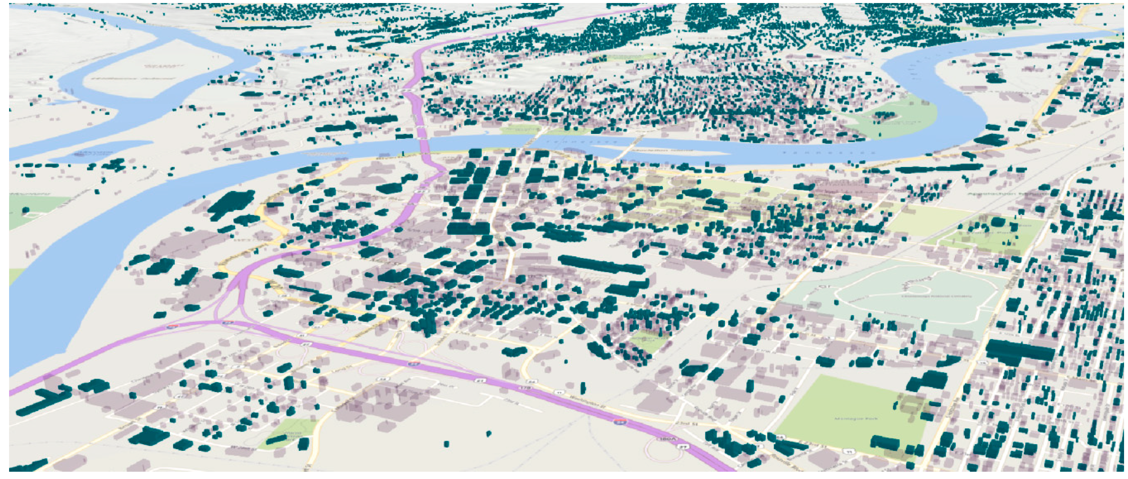
All buildings were converted to all-electric HVAC and water heating to define an upper-bound of maximum technical adoption potential. AutoBEM was used to create a unique baseline model for each of the 178,337 buildings captured in this study. Complicated measures (e.g., smart thermostat and smart water heater) leveraged OpenStudio measures to modify the models. For simpler measures (e.g., lighting and insulation), a C++ executable using faster text matching and string replacement was created and used to modify the model parameters. Simulation-based results including EUI, CO2 emissions, annual energy, annual demand, and energy/demand/cost savings for each building technology (individually and in aggregate) is provided publicly for each building in an updatable web platform (Figure 1).
4. Simulation and Analysis
There is a relatively broad and mature field of study which extends and leverages building energy modeling software to enable performance simulation for energy efficient technologies in the context of whole-building operation. Even prior to the increasing proliferation of urban-scale energy modeling studies, scalable application of technology measures in different building types, locations, and vintages for the purposes of building codes and standards was, and remains, a well-established use case that significantly impacts long-term energy use of the building stock [2,3,4,5]. Such use cases typically involve hundreds to thousands of individual models. Extending this to the hundreds of thousands of individual models used in this study, both for application of the measures and simulation, was non-trivial and required developing new technologies for world-class high performance computing (HPC) resources.
The models were originally simulated using Oak Ridge National Laboratory’s Titan, the world’s fastest supercomputer at the time of this project. A licensable software was created to handle the distribution and simulation of the models on High Performance Computing (HPC) resources called AutoSIM. This software demonstrated scalability for performing 524,288 annual simulations using 131,072 compute cores and writing 45 TB of data to permanent storage in 68 min. With the stated HPC resource and software pipeline constructed, the 178,337 models can be created, modified, simulated, transferred, analyzed, and summarized with interactive visualization tools online in less than 6.5 h. This software was then deployed on Argonne National Laboratory’s Theta supercomputer. Theta, the world’s 34th fastest supercomputer at the time of this writing, is focused primarily on Central Processing Units (CPU) rather than Graphical Processing Units (GPUs). DOE’s EnergyPlus simulation engine also primarily leverages CPUs rather than GPUs. As such, AutoSIM leveraged 114,688 compute cores to simulate 458,752 buildings (the equivalent of this utility for 2.5 technologies) and write 880 GB of results to disk in 28 min. Such HPC resources are publicly funded and can be acquired by anyone, anywhere, if an application is made detailing a sufficiently compelling scientific problem and computational readiness for such a resource. The baseline simulation results with AMY weather from 2015 were compared to each building’s 15 min electricity data from that year to ensure the models were of sufficient quality [32].
5. Results
Urban-scale building energy modeling is growing quickly and offering increasingly compelling capabilities for assessing demand-savings opportunities or evaluation of new business models for utilities, independent energy savings estimates for building owners, or actionable roadmaps for cities’ sustainability plans. In this study, we started by simply summarizing the number of buildings that could benefit from the technologies discussed. For each measure, there were a number of buildings in which the measure resulted in an increase in energy or demand. These buildings were omitted from the measure-aggregated results reported. The number of positive energy and demand savings observations for the reported distributions are summarized in Table 6.
5.1. Peak Contribution
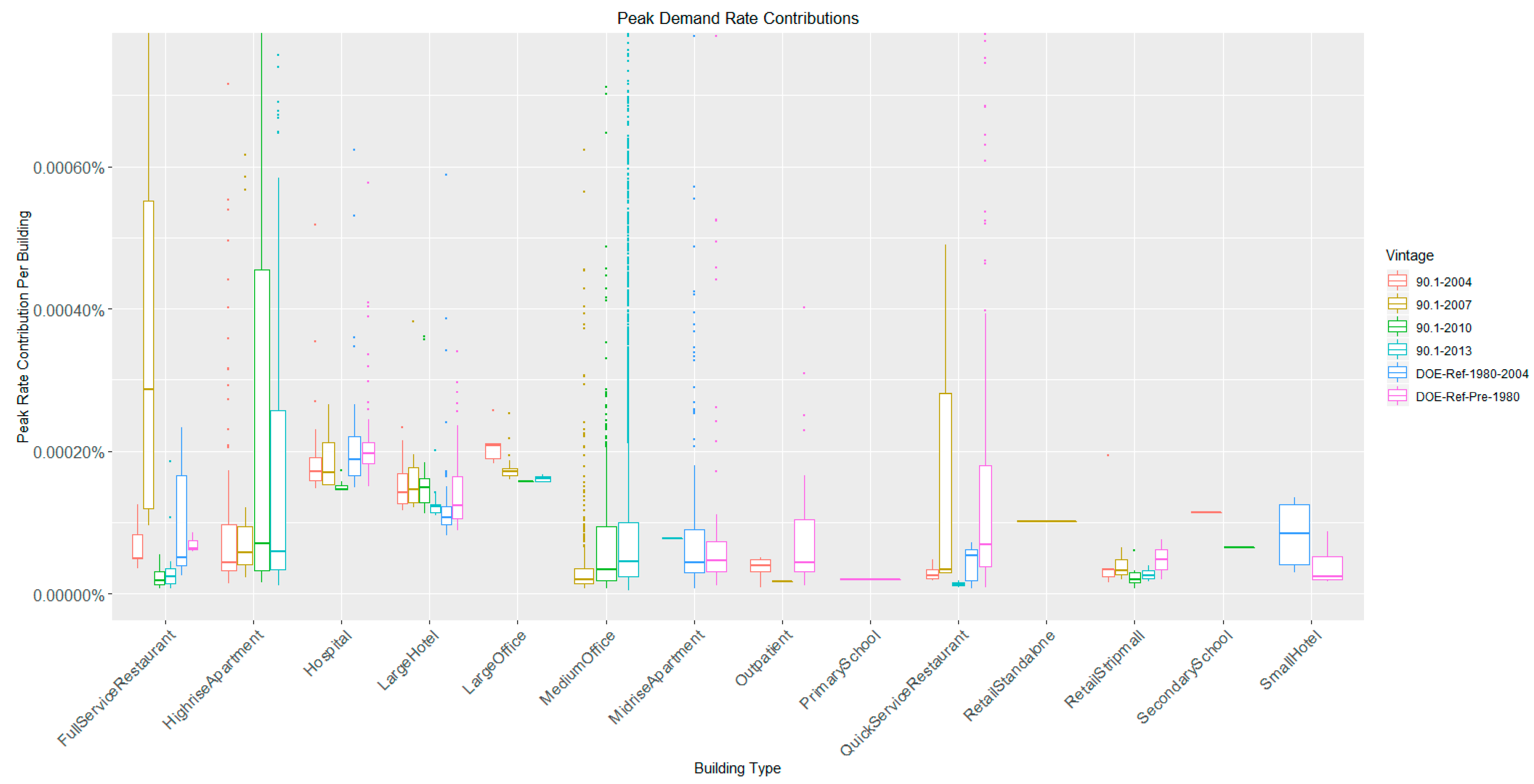
As previously described regarding customer empowerment, there was interest by the utility in breaking down contributions of each building to the peak hours of generation and provide some comparison of each building’s EUI to similar buildings (i.e., same type and vintage). Breaking down the peak demand contribution by building type and vintage can allow a utility to better formulate an energy efficiency program to target buildings and vintages that are disproportionate contributors to the dirtiest and most expensive hour of generation. As one might expect, larger buildings such as hospital, large hotel, and large office have the highest average peak demand reduction potential per building (result not shown for brevity). However, when accounting for the number of buildings, more common buildings with high energy intensity use such as restaurants, apartments, and medium offices become the primary contributors.
In Figure 2, box-and-whisker plots are used where the line in the middle indicates the median, the bottom and top of the rectangle are the lower/25th quartile and upper/75th quartile (meaning 25% and 75% of the data points lie below those values, respectively), and then the solid line indicates min and max while not accounting for outliers (individual dots). Since this study involves 178,377 premises, if every building contributed equally to demand, all data would lie on a line with y-axis of 0.000005607%. However, with a unit of 0.0001%, buildings at this level would contribute 18× more toward peak than such an average building. In this figure, in an attempt to make the distributions visible, some outliers are not represented even though those buildings have the best technical adoption potential for demand management. Likewise, flat lines indicate building type-vintage combinations where there was not a significant number of buildings (e.g., PrimarySchool). There are more buildings of these types within the region, but are not assigned as such since their energy use profile more closely matches another building type and vintage combination.
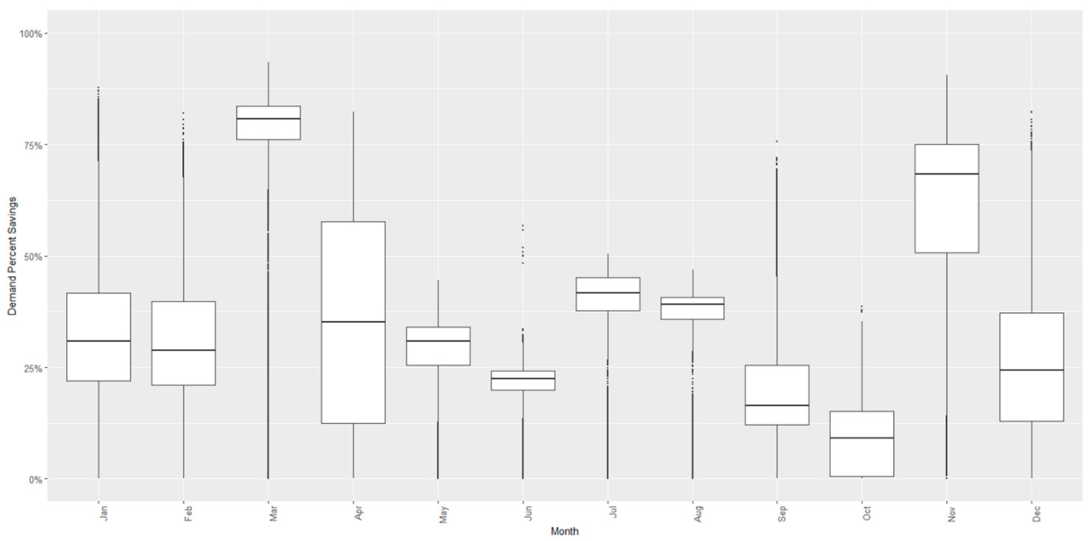
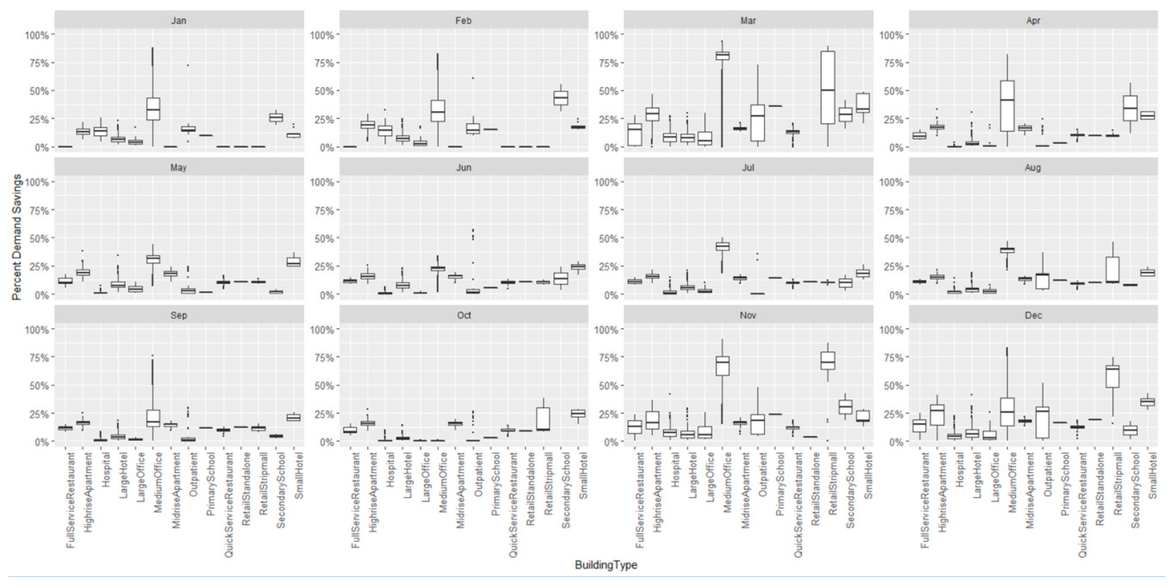
While utility programs may target specific building types, there is also a temporal dimension to consider (Figure 3) where peak management may not be the same in summer and winter months, that is, the most cost-effective demand management technique may vary by building type, vintage, technology, and monthly weather.
5.2. Demand Side Management
Smart thermostats, for pre-conditioning buildings as thermal batteries prior to peak hour demand, is among the traditional demand management technologies that may be cost effective for utility programs to implement. While utility-managed thermostats can lower energy, demand, emissions, and costs for the utility, these are often passed on, either directly or indirectly, to the program participant or rate payer. Additionally, technologies such as smart thermostat settings that could affect comfort always allow setpoint override so as not to participate at that time. Figure 4 shows the wide range of potential demand savings for over 100,000 buildings under a maximum technical adoption scenario where the percentage reported is the percent of kW during the building’s peak that could be reduced through pre-conditioning.
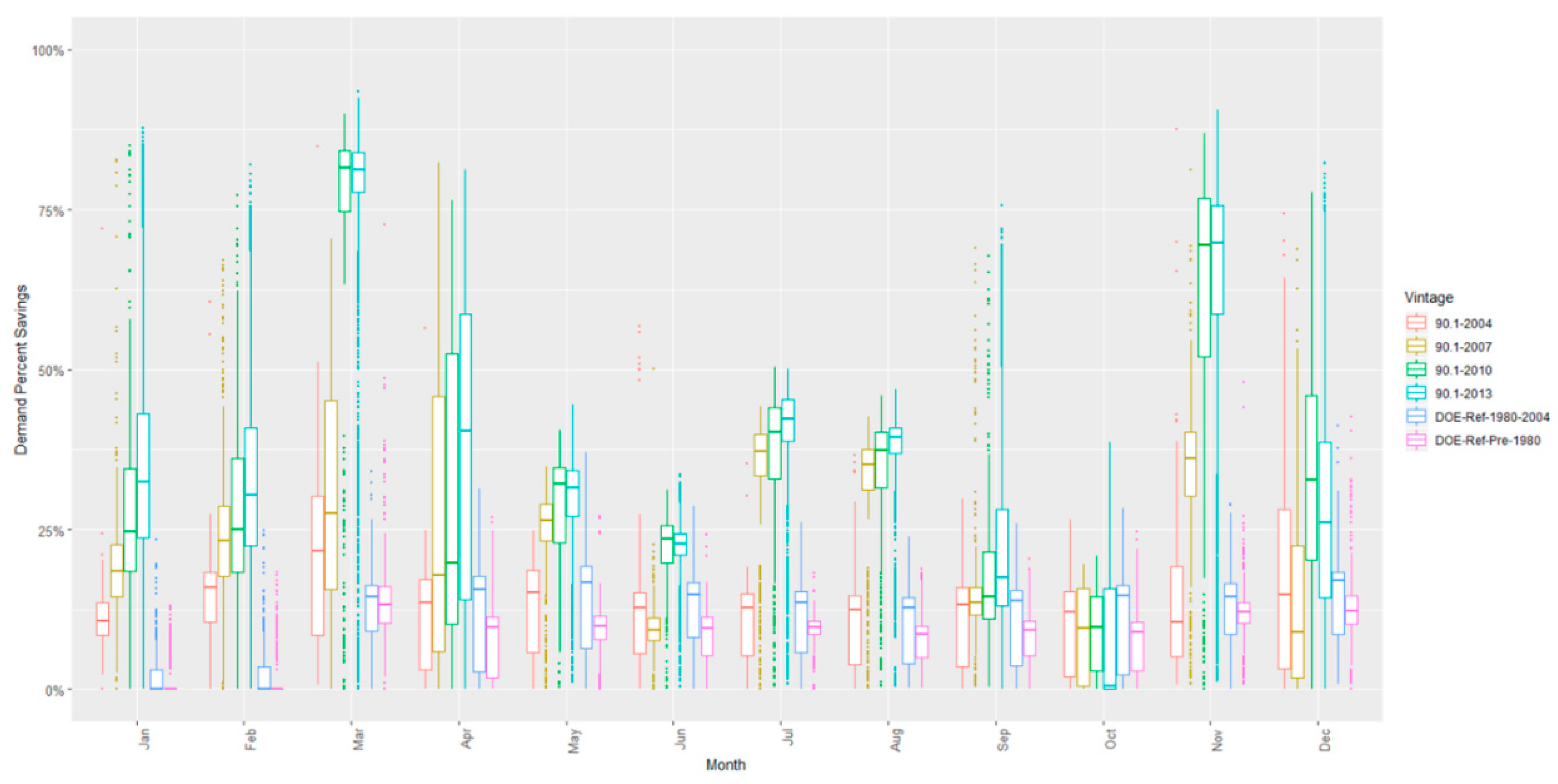
Figure 5 and Figure 6 demonstrate the power of building-specific, bottom-up aggregation to allow visual analytics of demand savings by vintage or building type. In these figures, demand reduction is instead a percentage of kW reduction for the entire service territory. As an example, March and November with vintages of 90.1-2010 and 90.1-2013 are relatively high due to the lower energy demand during those shoulder months combined with the fact that those are the two most popular vintages of buildings in the utility’s service territory.
Smart thermostat savings opportunities grouped by building type explain the aggregate results even more thoroughly. Again March and November have significantly more savings opportunities in the medium office of which there are many in the EPB service area. The other building type with significant demand savings potential is the retail stripmall.
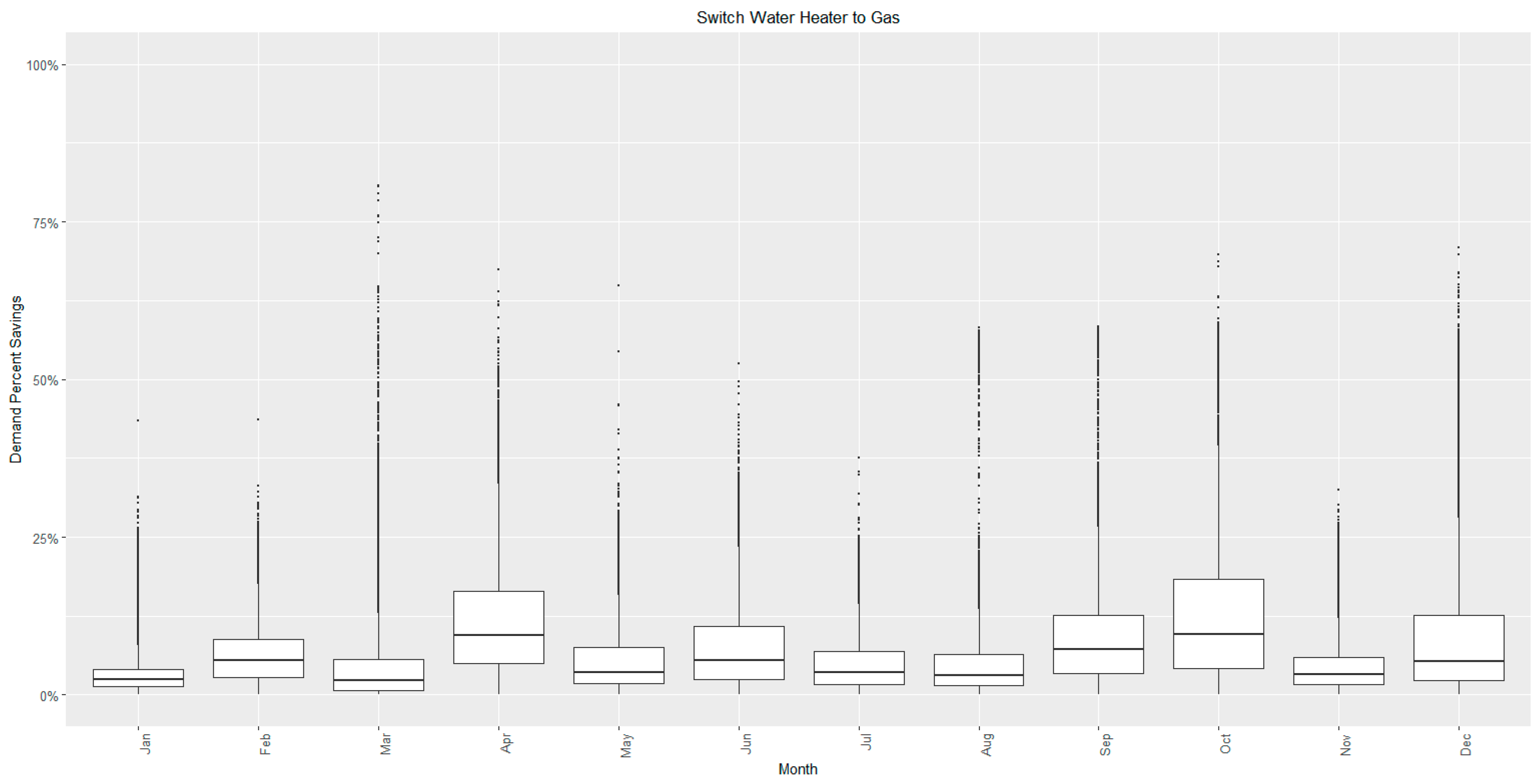
Switching a building’s water heater from electric to natural gas or other fuel type is another strategy that could reduce peak electric demand. This study indicates the greatest savings opportunities (Figure 7) in the utility’s service territory for such a strategy in April and October.
HVAC systems can also be changed from electricity to natural gas for heating. In fact, there are dual-fuel systems that offer additional resilience with the potential for a utility-controlled signal to request the equipment dynamically swap between electricity or natural gas for heating. Such a demand management strategy will be most effective in the winter months. Results, shown in Figure 8, indicate that older buildings have the greatest average savings potential throughout the winter and even have some savings opportunity in the summer. Newer buildings have close to zero savings opportunity in the summer and much lower savings opportunities in the winter months with greater savings potential from older commercial vintages (90.1-2004). While not shown here, the study found Quickservice restaurants to be the only building type that consistently showed potential demand savings from this strategy during summer months.
5.3. Energy Efficiency
While demand management remains one of the biggest opportunities for today’s utilities, traditional energy efficiency remains one of the most cost-effective opportunities for long-term savings for building owners. In the utility’s territory, if the system-wide annual bill was shared equally among all buildings and cost USD 5 per year, USD 1 would be for demand and USD 4 for energy.
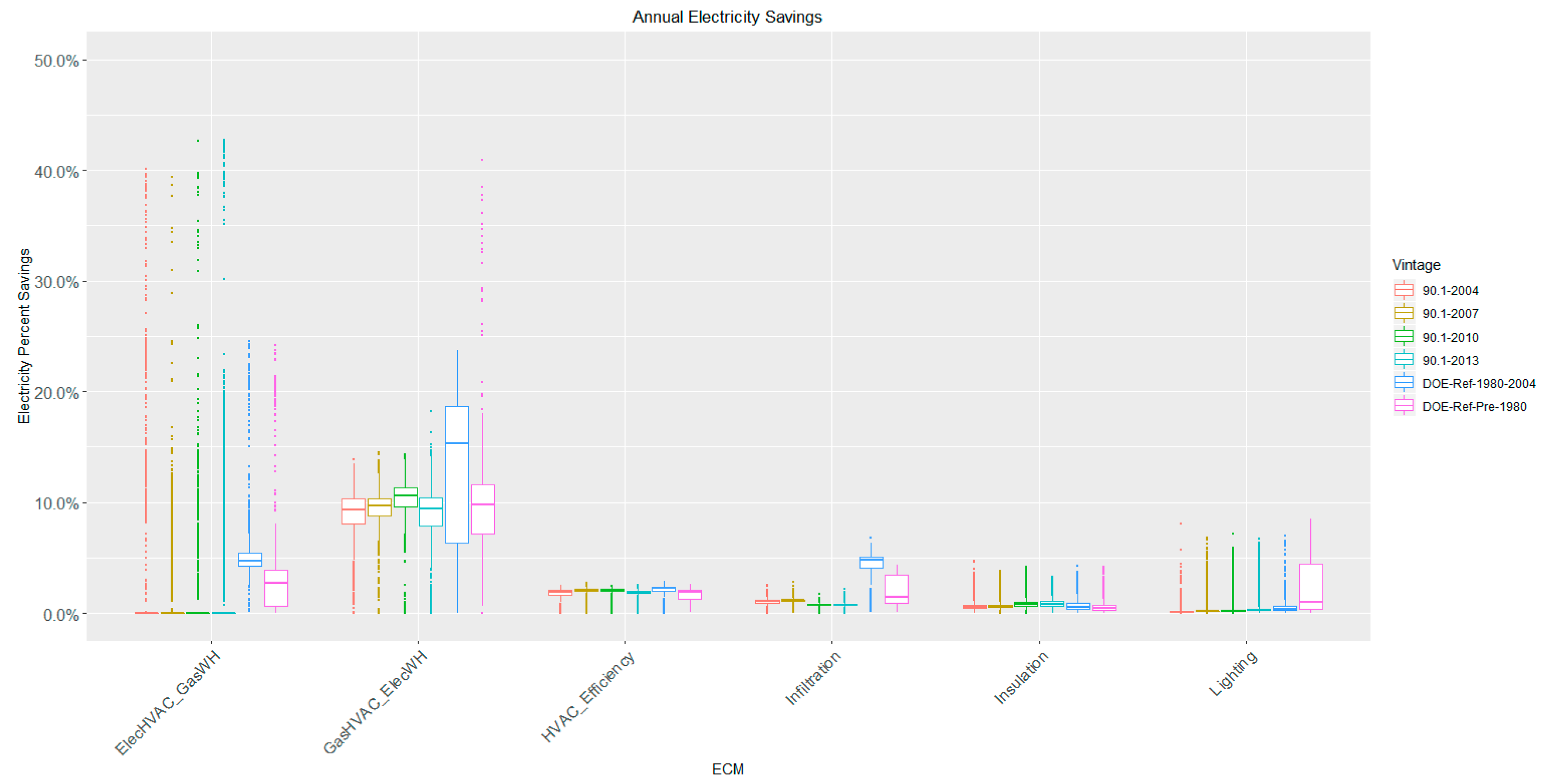
Technologies 1–6, presented initially in Table 2, are among the most common and cost-effective building energy efficiency measures considered. Annual electricity savings by vintage are shown in Figure 9. It should be noted that swapping the water heater or HVAC (two columns on the left) results in higher electricity energy savings by shifting related costs to other fuel types. This study shows that the oldest buildings have the most electricity savings potential. While not shown here, preliminary results from the study indicate that annual electricity savings are greatest for newer vintages when considering only commercial buildings.
From a total energy and cost perspective, the traditional energy efficiency measures of a more efficient HVAC (typically at end-of-life), reducing infiltration (sealing leaks between the indoors and outdoors), adding insultation (further reducing conductive heat transfer), and swapping to more efficient lighting technologies, often are at the top of most building efficiency discussions.
5.4. Emissions
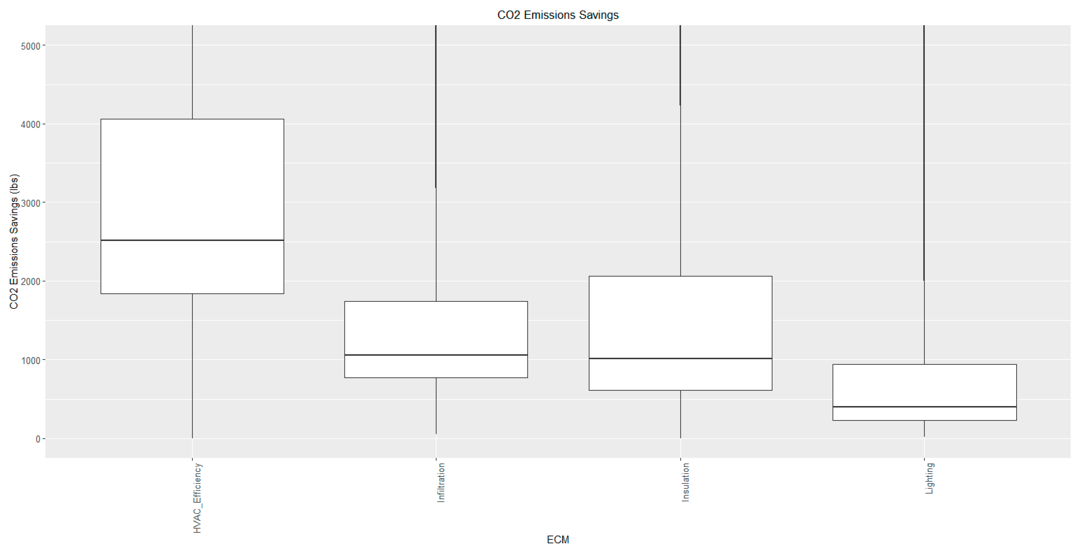
Long-term environmental impact of the building stock may be better considered via greenhouse gas emissions required for the creation and operation of a building. Many activities relevant to urban-scale energy modeling are in service of individual cities defining sustainability plans with activities for curbing emissions of buildings and vehicles. In this study, annual emissions savings were calculated directly from annual electricity savings using EPA’s eGRID [27] and thus identical except for lbs/MWh scaling factor and resulting emissions unit. In reality, peak demand electricity generation often has higher emissions than typical generation so peak demand shaving would result in higher values of emissions savings. This is not accounted for in this analysis. Changing from electric to gas ECMs is also not shown in the emissions figure, as the total savings from reducing electricity savings would not be realized as gas would entail emissions as well. As all emission plots are similar in shape with a different scale, only CO2 emissions are shown in Figure 10.
5.5. Cost Savings
While demand, energy, and emissions vary considerably in relative importance by stakeholder, almost all stakeholders consider potential cost savings. In these results, retail-rate electricity cost savings were calculated using the US national average for 2015 of USD 0.1041/kWh and USD 10.5/kW. Since residential buildings largely do not elect a demand-sensitive (e.g., time-of-use) pricing structure, these results show limited cost savings for demand response compared to annual electricity savings. The utility-wide total potential retail cost savings for both electricity and demand of each technology is shown in Figure 11. It should be noted that not all savings could be realized for the switch from electricity to gas as the additional cost of gas, and concomitant potential loss of revenue for the utility, is not considered here.
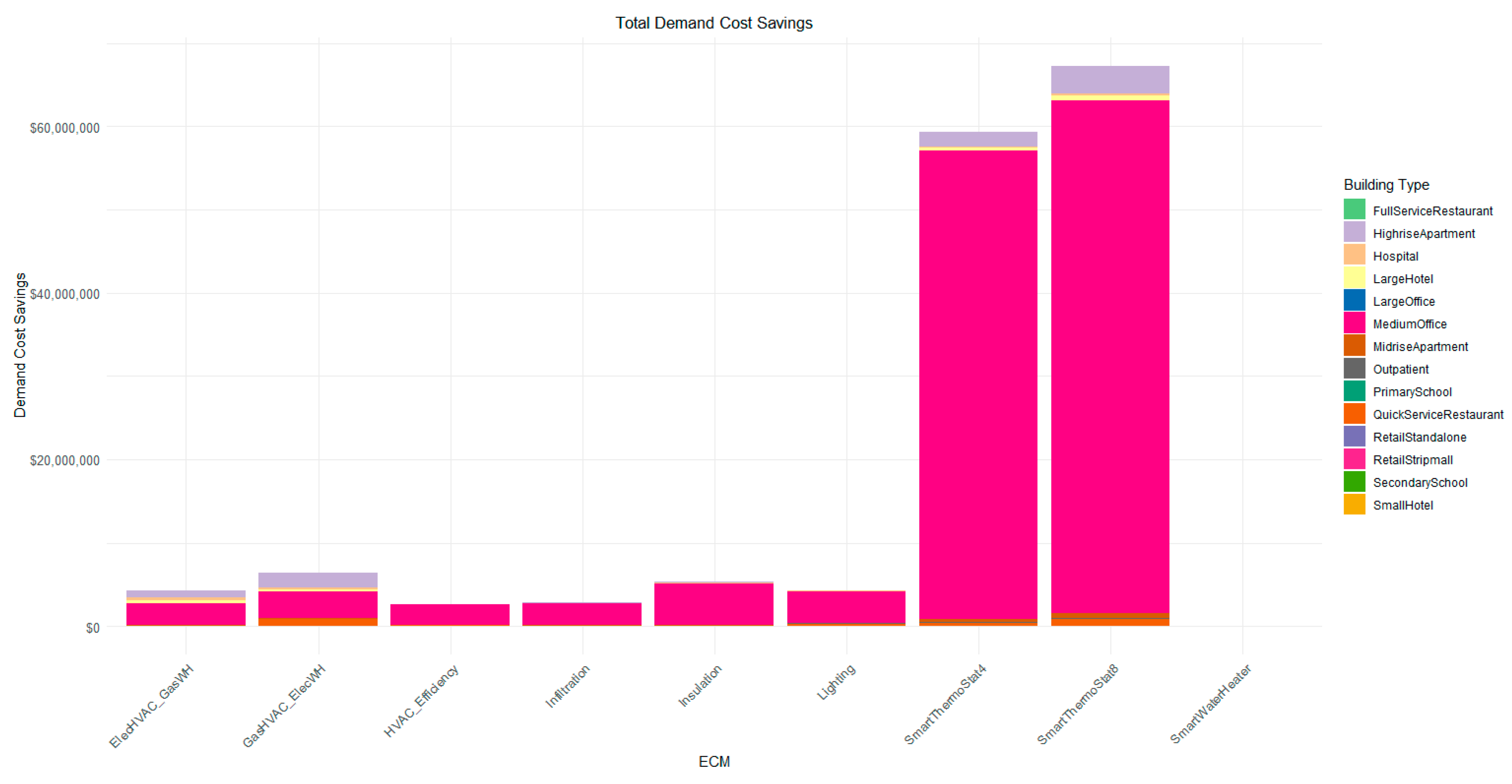
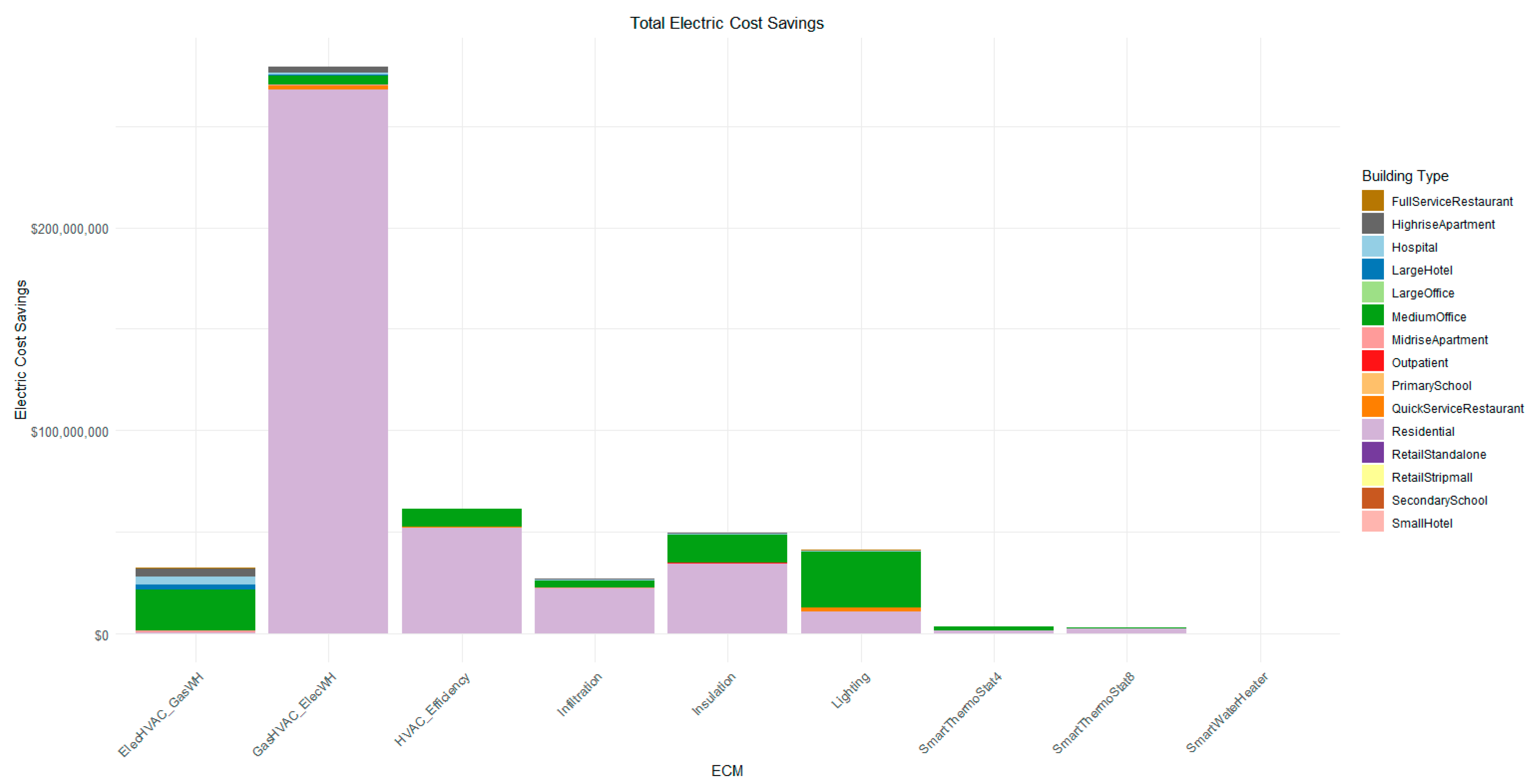
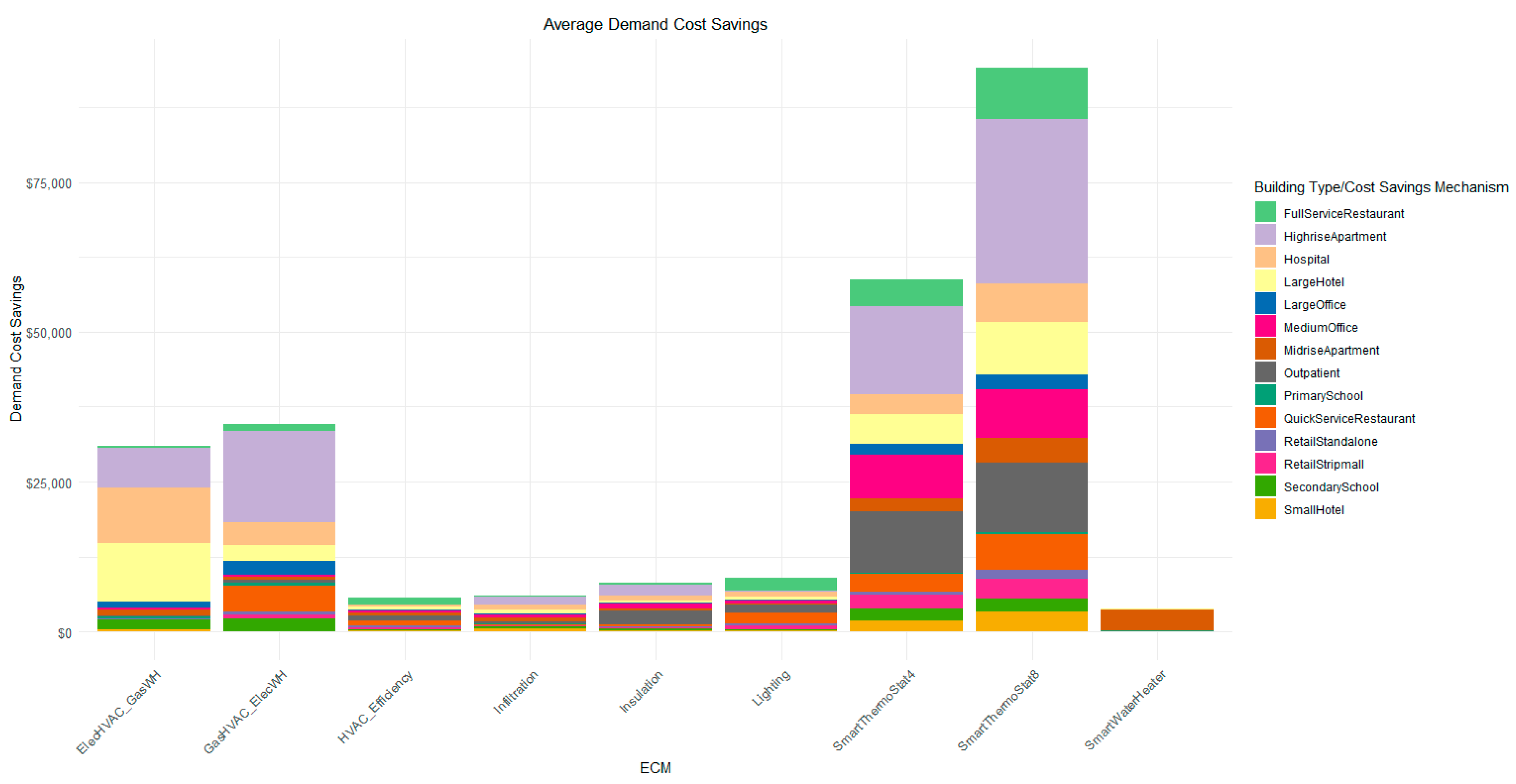
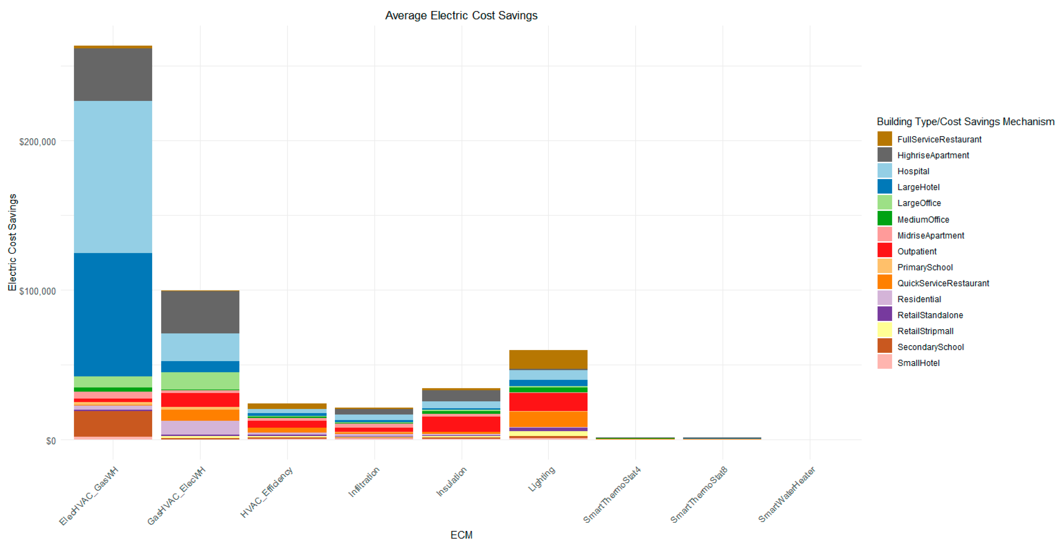
While Figure 11, Figure 12 and Figure 13 constitute business intelligence that can lead to long-term program formulation and utility activities, the domination of individual building types at utility-scale can obfuscate the short-term, per-building cost effectiveness for deployment. Figure 14 and Figure 15 normalize the demand and energy potential cost savings, respectively, while normalizing for number of buildings to achieve the savings that could be seen at an individual building. In these results, it may be interesting to note reversal of trends from the totals. For example, switching to a gas water heater is actually a more effective cost reduction than switching to gas HVAC, while the totals indicated the opposite. High-rise apartments appear to be excellent candidates for demand-related cost savings for several measures. When considering energy-related cost savings, switching to a gas water heater has a significant amount of savings in large hotel buildings as well as hospitals. Lighting efficiency is estimated to have the greatest average potential savings opportunity for quick-service restaurants, outpatients, and full-service restaurants. However, since there are particular building types that lack a significant number of actual buildings in the utility’s service area, these averages may be biased.
In addition to demand- and energy-related cost savings, many older buildings may be reaching end-of-life for existing equipment or ready for a retrofit to modernize/upgrade the building, further increasing the timeliness and likelihood of deployment for energy efficient building technologies. Figure 16 and Figure 17 show similar average per-building potential cost savings for demand and energy, respectively, broken down by vintage. Generally, and perhaps counter-intuitively, older buildings are estimated to have lower demand savings potential for most technologies other than gas HVAC swapout for DOE-Ref-Pre-1980. In contrast to previous results, there are some cost savings for the smart water heater ECM, the DOE-Ref-1980-2004 vintage in particular had savings.
6. Summary
While there are currently a plethora of data sources, algorithms, software packages, and capable people behind the scientific and technological advancements, urban-scale energy modeling still has much to gain from cross-study comparative analysis as well as empirical validation against measured energy sources and building details before maturing toward the establishment of best practices and guidelines. In this study, a utility’s top five use cases and nine monetization scenarios for a digital twin of buildings were reported. OpenStudio and EnergyPlus empirically validated building energy models of 178,337 buildings were constructed and used to assess the maximum technical adoption potential for distributions of energy, demand, emissions, and cost savings of several building technologies. For brevity, only eight measures and a limited set of results summarizing distributions of various performance metrics by month, vintage, and building type for some of these measures were discussed.
For the limited set of eight energy efficient building technologies evaluated, the authors found energy savings in 99% and demand savings in 78% of the 100,000+ buildings included in this study. Combining residential and commercial energy savings, an average 7.5% COP increase in HVAC efficiency resulted in a per-building electrical savings of 270 kWh and annual energy costs of USD 28,500, when averaged across 177,307 buildings. For demand savings, 2.2 °C of building pre-conditioning 2 h before peak hour has the potential to save an average of 27% of a building’s demand and annual demand costs of USD 5200, but varied from 0 to 93% over a sample of 101,082 buildings. When taken individually, improved HVAC efficiency, space sealing, insulation, or lighting have the potential to offset 500 to 3000 lbs. of CO2 per building. This study provides detailed breakdowns by month, building type, vintage, in aggregate, and at the per-building level to facilitate use by utility efficiency programs, sustainability officers, and those making investment decisions in upgrading the nation’s building stock.
Significant demand savings were available in the transition months (March/November) for smart thermostats, while changing water heaters from electric to gas had the greatest savings potential in April and October. Changing HVAC from electricity to gas offers significant demand savings throughout the winter for previously electrically heated buildings. The majority of energy efficiency savings came from older vintages with greater room for efficiency improvement. Regarding cost, electricity cost savings dominated demand cost savings for all ECMs other than the smart thermostats.
The authors are hopeful that such results will be useful for comparison with other studies involving explicit data, distributions, or evolving metrics of urban-scale building characteristics, energy use, end use loads demand management (especially synergies/tradeoffs), emissions reductions, or estimated savings.
Author Contributions
Conceptualization, J.N. and W.C.; methodology, J.N.; software, B.B.; validation, W.C.; resources, J.N.; data curation, J.N., W.C., and B.B.; writing—original draft preparation, J.N. and B.B.; writing—review and editing, W.C.; visualization, B.B.; supervision, J.N.; project administration, J.N.; funding acquisition, J.N. and W.C. All authors have read and agreed to the published version of the manuscript.
Funding
This work was funded by field work proposal CEBT105 under US Department of Energy Building Technology Office Activity Number BT0305000, as well as Office of Electricity Activity Number TE1103000.
Acknowledgments
The authors would like to thank Amir Roth and Madeline Salzman for their support and review of this project. The authors would also like to thank Mark Adams for his contributions to the AutoBEM software for model generation, Jibonananda Sanyal for AutoSIM contributions for scalable simulation, and Tianjing Guo for implementation of measures used in this study.
Conflicts of Interest
This manuscript was authored by UT-Battelle, LLC under Contract No. DE-AC05-00OR22725 with the U.S. Department of Energy. The United States Government retains and the publisher, by accepting the article for publication, acknowledges that the United States Government retains a non-exclusive, paid-up, irrevocable, world-wide license to publish or reproduce the published form of this manuscript or allow others to do so, for United States Government purposes. The Department of Energy will provide public access to these results of federally sponsored research in accordance with the DOE Public Access Plan (http://energy.gov/downloads/doe-public-access-plan).
References
- Building Technologies Office Multi-Year Program Plan, Fiscal Years 2016–2020; US Department of Energy: Washington, DC, USA, 2016.
- Cerezo, C.; Sokol, J.; AlKhaled, S.; Reinhart, C.; Al-Mumin, A.; Hajiah, A. Comparison of four building archetype characterization methods in urban building energy modeling (UBEM): A residential case study in Kuwait City. Energy Build. 2017, 154, 321–334. [Google Scholar] [CrossRef]
- Sokol, J.; Cerezo Davila, C.; Reinhart, C.F. Validation of a Bayesian-based method for defining residential archetypes in urban building energy models. Energy Build. 2017, 134, 11–24. [Google Scholar] [CrossRef]
- Nutkiewicz, A.; Yang, Z.; Jain, R.K. Data-driven Urban Energy Simulation (DUE-S): A framework for integrating engineering simulation and machine learning methods in a multi-scale urban energy modeling workflow. Appl. Energy 2018, 225, 1176–1189. [Google Scholar] [CrossRef]
- Cerezo Davila, C.; Reinhart, C.F.; Bemis, J.L. Modeling Boston: A workflow for the efficient generation and maintenance of urban building energy models from existing geospatial datasets. Energy 2016, 117, 237–250. [Google Scholar] [CrossRef]
- Deru, M.; Field, K.; Studer, D.; Benne, K.; Griffith, B.; Torcellini, P.; Liu, B.; Halverson, M.; Winiarski, D.; Rosenberg, M.; et al. U.S. Department of Energy Commercial Reference Building Models of the National Building Stock; NREL/TP-5500-46861; National Renewable Energy Laboratory: Lakewood, CO, USA, 2011. [Google Scholar]
- Commercial Reference Buildings. Energy.gov. n.d. Available online: https://www.energy.gov/eere/buildings/commercial-reference-buildings (accessed on 5 October 2020).
- Commercial Prototype Building Models. 2018. Available online: https://www.energycodes.gov/development/commercial/prototype_models (accessed on 17 October 2020).
- ASHRAE. Climatic Data for Building Design Standards; ASHRAE Standard 169-2013; ASHRAE: Atlanta, GA, USA, 2013. [Google Scholar]
- ASHRAE. Energy Standard for Buildings Except Low-Rise Residential Buildings; Standard 90.1-2019; ASHRAE: Atlanta, GA, USA, 2019. [Google Scholar]
- Lee, S.H.; Hong, T.; Sawaya, G.; Chen, Y.; Piette, M.A. DEEP: A Database of Energy Efficiency Performance to Accelerate Energy Retrofitting of Commercial Buildings; LBNL-180309; Lawrence Berkeley National Laboratory: Berkeley, CA, USA, 2015. [Google Scholar]
- Levine, M.; Feng, W.; Ke, J.; Hong, T.; Zhou, N. A Retrofit Tool for Improving Energy Efficiency of Commercial Buildings. In Proceedings of the 2012 ACEEE Summer Study on Energy Efficiency in Buildings, Pacific Grove, CA, USA, 12–17 August 2012; Volume 3, pp. 213–224. [Google Scholar]
- Wang, N.; Goel, S.; Srivastava, V.; Makhmalbaf, A. Building Energy Asset Score, Program. Overview and Technical Protocol (Version 1.2); PNNL-22045 Rev. 1.2; Pacific Northwest National Laboratory: Richland, WA, USA, 2015.
- Karpman, M.; Wang, N.; Eley, C.; Goel, S. Comparative Analysis of ASHRAE Building EQ As-Designed, DOE Building Energy Asset Score and ASHRAE 90.1 Performance Rating Method Asset Ratings. In Proceedings of the Building Simulation 2017, San Francisco, CA, USA, 7–9 August 2017. [Google Scholar]
- Roth, A.; Brackney, L.; Parker, A.; Beitel, A. OpenStudio: A Platform for Ex Ante Incentive Programs. In Proceedings of the 2016 ACEEE Summer Study on Energy Efficiency in Buildings, Pacific Grove, CA, USA, 21–26 August 2016; Volume 4, pp. 1–12. [Google Scholar]
- Scout. Energy.gov. n.d. Available online: https://www.energy.gov/eere/buildings/scout (accessed on 20 October 2020).
- Roth, A. Building Energy Modeling 101: Stock-Level Analysis Use Case. 18 April 2017. Available online: https://www.energy.gov/eere/buildings/articles/building-energy-modeling-101-stock-level-analysis-use-case (accessed on 22 October 2020).
- Wang, N.; Makhmalbaf, A.; Srivastava, V.; Hathaway, J.E. Simulation-Based Coefficients for Adjusting Climate Impact on Energy Consumption of Commercial Buildings. Build. Simul. 2017, 10, 309–322. [Google Scholar] [CrossRef]
- Ng, L.C.; Quiles, N.O.; Dols, W.S.; Emmerich, S.J. Weather Correlations to Calculate Infiltration Rates for U. S. Commercial Building Energy Models. Build. Environ. 2018, 127, 47–57. [Google Scholar] [CrossRef] [PubMed]
- Shrestha, S.; Hun, D.; Ng, L.; Desjarlais, A.; Emmerich, S.; Dalgliesh, L. Online Airtightness Savings Calculator for Commercial Buildings in the US, Canada and China. In Proceedings of the Thermal Performance of the Exterior Envelopes of Whole Buildings XIII International Conference, Clearwater Beach, FL, USA, 4–8 December 2016; pp. 152–160. [Google Scholar]
- Irwin, R.; Chan, J.; Frisque, A. Energy Performance for ASHRAE 90.1 Baselines for a Variety of Canadian Climates and Building Types; Stantec Consulting Ltd.: Vancouver, BC, Canada, 2016. [Google Scholar]
- IECC. International Energy Conservation Code 2012. C403(2). Available online: https://codes.iccsafe.org/content/IECC2012 (accessed on 24 October 2020).
- ICF International. Seal and Insulate with ENERGY STAR® Savings Analysis Measure Upgrade Assumptions. (I. I. STAR®, Producer). 2014. Available online: https://www.energystar.gov/ia/home_improvement/home_sealing/Measure_Upgrade_Assumptions.pdf (accessed on 25 October 2020).
- Guglielmetti, R.; Macumber, D.; Long, N. OpenStudio: An Open Source Integrated Analysis Platform. In Proceedings of the Building Simulation, Sydney, Australia, 14–16 November 2011. Preprint NREL/CP-5500-51836. [Google Scholar]
- Crawley, D.B. EnergyPlus: Creating a new-generation building energy simulation program. Energy Build. 2001, 33, 319–331. [Google Scholar] [CrossRef]
- Roth, A. New OpenStudio-Standards Gem Delivers One Two Punch. 15 September 2016. Available online: https://www.energy.gov/eere/buildings/articles/new-openstudio-standards-gem-delivers-one-two-punch (accessed on 25 October 2020).
- U.S. EPA. Emissions & Generation Resource Integrated Database (eGRID). 2017. Available online: https://www.epa.gov/energy/emissions-generation-resource-integrated-database-egrid (accessed on 28 October 2020).
- New, J.R.; Adams, M.; Im, P.; Yang, H.; Hambrick, J.; Copeland, W.; Bruce, L.; Ingraham, J. Automatic Building Energy Model Creation (AutoBEM) for Urban-Scale Energy Modeling and Assessment of Value Propositions for Electric Utilities. In Proceedings of the International Conference on Energy Engineering and Smart Grids (ESG), Cambridge, UK, 25–26 June 2018. [Google Scholar]
- New, J.R.; Bhandari, M.; Shrestha, S.; Allen, M. Creating a Virtual Utility District: Assessing Quality and Building Energy Impacts of Microclimate Simulations. In Proceedings of the International Conference on Sustainable Energy and Environmental Sensing (SEES), Cambridge, UK, 18–19 June 2018. [Google Scholar]
- Dogan, T.; Reinhart, C.; Michalatos, P. Autozoner: An algorithm for automatic thermal zoning of buildings with unknown interior space definitions. J. Build. Perform. Simul. 2015, 9, 1–14. [Google Scholar] [CrossRef]
- Smith, L.; Bernhardt, K.; Jezyk, M. Automated energy model creation for conceptual design. In Proceedings of the 2011 Symposium on Simulation for Architecture and Urban Design Society for Computer Simulation International, Boston, MA, USA, 3–7 April 2011; pp. 13–20. [Google Scholar]
- Garrison, E.; New, J.R.; Adams, M. Accuracy of a Crude Approach to Urban Multi-Scale Building Energy Models Compared to 15-min Electricity Use. In Proceedings of the ASHRAE Winter Conference, Atlanta, GA, USA, 12–16 January 2019. Ph.D. Student Paper award. [Google Scholar]
Figure 1.
All 178,337 buildings and simulation results can be searched, selected, and visualized using flexible regular expressions that can query and combine any number of data fields (bit.ly/virtual_epb).
Figure 1.
All 178,337 buildings and simulation results can be searched, selected, and visualized using flexible regular expressions that can query and combine any number of data fields (bit.ly/virtual_epb).

Figure 2.
Box-and-whisker plot indicates statistical distribution of each building’s contribution to the utility’s twelve monthly peak hours added together, broken down by building type and vintage.
Figure 2.
Box-and-whisker plot indicates statistical distribution of each building’s contribution to the utility’s twelve monthly peak hours added together, broken down by building type and vintage.

Figure 3.
Distribution of potential demand contribution by building type for each month.

Figure 4.
Smart thermostats with utility-signaled 2.2 °C of building pre-conditioning 2 h before peak hour has the potential to save an average of 27% of a building’s demand, but this sample of 101,082 buildings varies from 0–93% by individual building and time of year.
Figure 4.
Smart thermostats with utility-signaled 2.2 °C of building pre-conditioning 2 h before peak hour has the potential to save an average of 27% of a building’s demand, but this sample of 101,082 buildings varies from 0–93% by individual building and time of year.

Figure 5.
Potential demand reduction achievable with 2.2 °C pre-conditioning by building vintage.

Figure 6.
Potential monthly demand reduction achievable with 2.2 °C pre-conditioning by building type.
Figure 6.
Potential monthly demand reduction achievable with 2.2 °C pre-conditioning by building type.

Figure 7.
Changing water heaters from electricity to natural gas can relieve peak electric demand. This study found that a building’s demand could be reduced as much as 80% but averages approximately 5% of building peak.
Figure 7.
Changing water heaters from electricity to natural gas can relieve peak electric demand. This study found that a building’s demand could be reduced as much as 80% but averages approximately 5% of building peak.

Figure 8.
Distributions of potential demand reduction for a building, broken down by month and building vintage, achievable with swapping HVAC equipment from electricity to natural gas or dual-fuel equipment with a utility signal to reduce electricity use during peak hour.
Figure 8.
Distributions of potential demand reduction for a building, broken down by month and building vintage, achievable with swapping HVAC equipment from electricity to natural gas or dual-fuel equipment with a utility signal to reduce electricity use during peak hour.

Figure 9.
Distribution of potential annual electricity savings for two fuel-switching technologies (water heater and HVAC), and four traditional energy efficiency measures.
Figure 9.
Distribution of potential annual electricity savings for two fuel-switching technologies (water heater and HVAC), and four traditional energy efficiency measures.

Figure 10.
Distribution across buildings in the utility’s service area of operational emissions savings for four traditional energy efficiency measures.
Figure 10.
Distribution across buildings in the utility’s service area of operational emissions savings for four traditional energy efficiency measures.

Figure 11.
Combined utility-scale energy and demand annual retail-rate electricity cost savings.

Figure 12.
Medium office buildings, the most prevalent commercial building type, account for the majority of total, utility-scale, demand-related cost savings. Smart thermostats have very little or negative annual electricity savings.
Figure 12.
Medium office buildings, the most prevalent commercial building type, account for the majority of total, utility-scale, demand-related cost savings. Smart thermostats have very little or negative annual electricity savings.

Figure 13.
Residential and medium office commercial buildings, due to number of buildings, dominate utility-scale potential electricity cost savings.
Figure 13.
Residential and medium office commercial buildings, due to number of buildings, dominate utility-scale potential electricity cost savings.

Figure 14.
Average demand-related electricity cost savings by building type can indicate cost-conscious opportunities for short-term wins in demand management.
Figure 14.
Average demand-related electricity cost savings by building type can indicate cost-conscious opportunities for short-term wins in demand management.

Figure 15.
Average energy-related electricity cost savings by building type are on average 4× higher than demand-related savings and typically offer the best cost savings for building owners.
Figure 15.
Average energy-related electricity cost savings by building type are on average 4× higher than demand-related savings and typically offer the best cost savings for building owners.

Figure 16.
Average demand-related electricity cost savings by building vintage can indicate cost-conscious opportunities for short-term wins in demand management.
Figure 16.
Average demand-related electricity cost savings by building vintage can indicate cost-conscious opportunities for short-term wins in demand management.

Figure 17.
Average energy-related electricity cost savings potential by building vintage indicates significant savings opportunities. By combining building type and vintage for energy and demand, an initial estimate of cost savings can be used to determine if purchase and installation of these technologies may be cost-effective.


Table 1.
Use cases and potential sources of savings considered in this study for each building technology further defined in Table 2.
Table 1.
Use cases and potential sources of savings considered in this study for each building technology further defined in Table 2.
| Number | Use Case | Monetization |
|---|---|---|
| 1a | Peak Rate Structure | Identify buildings that contribute disproportionately to energy/demand costs |
| 1b | Peak Rate Structure | Quantify wholesale vs. retail cost/year for all buildings under different rate structures |
| 2a | Demand Side Management | Monthly peak demand savings, annual energy savings, and dollar savings based on rate structure for each building |
| 2b | Demand Side Management | Location-specific deferral of infrastructure (e.g., feeder, substation) cost savings potential |
| 3 | Emissions | Emissions footprints for each building |
| 4a | Energy Efficiency | Optimal retrofit savings of each independent building technology |
| 4b | Energy Efficiency | Optimal retrofit package savings of dependent building technologies |
| 5a | Customer Empowerment | Percentile ranking of each building’s Energy Use Intensity for similar building type and vintage |
| 5b | Cost Savings | Monthly peak demand savings, annual energy savings, and dollar savings based on rate structure for each building |
Table 2.
Building technologies/controls (measures) simulated in each of the 178,337 building energy models to quantify savings defined in Table 3. Acronyms: IECC (International Energy Conservation Code), HVAC (Heating, Ventilation, and Air Conditioning).
Table 2.
Building technologies/controls (measures) simulated in each of the 178,337 building energy models to quantify savings defined in Table 3. Acronyms: IECC (International Energy Conservation Code), HVAC (Heating, Ventilation, and Air Conditioning).
| Number | Description | Category | Values | Source |
|---|---|---|---|---|
| 1 | Insulate Roof | Envelope | R-16.12 to R-28.57 | IECC-2012 [22] |
| 2 | Reduce Space Infiltration | Envelope | Reduce 25% from building vintage | EnergyStar whole-house [23] |
| 3 | Smart Thermostat (2.2 °C) | HVAC | 2.2 °C, 2 h prior to peak | Utility request |
| 4 | Smart Thermostat (4.4 °C) | HVAC | 4.4 °C, 4 h prior to peak | Utility request |
| 5 | Change Electric HVAC COP | HVAC | COP to 3.55 (heating) 3.2 (cooling) | IECC-2012 |
| 6 | Change Lighting Power Density | Lighting | LPD 0.85 W/ft2 | IECC-2012 |
| 7 | Change to Gas Water Heater | Water | Efficiency 80% (assumes electric baseline) | IECC-2012 |
| 8 | Change to Gas HVAC | HVAC | Efficiency 80% (assumes electric baseline) | IECC-2012 |
Table 3.
Consolidated simulation outputs calculated for each measure. Acronym: ECM (Energy Conservation Measure).
Table 3.
Consolidated simulation outputs calculated for each measure. Acronym: ECM (Energy Conservation Measure).
| Category | Description |
|---|---|
| building ID | Unique identifier of each building |
| electricity (kWh) | Total simulated electrical consumption. (Default: Annual, monthly, daily, 15 min unless stated otherwise) |
| demand (kW) | Total annual energy demand summed over building’s simulated monthly peaks. (Annual, monthly) |
| energy (GJ) | Total electricity + gas consumption |
| emissions (lbs) | Total emissions based on simulated energy use for Carbon Dioxide (CO2), Sulfur Dioxide (SO2), Nitrogen Oxides (NOx), Nitrous oxide (N2O), and Methane (CH4). |
| cost (USD) | Wholesale and retail costs combining simulated energy and demand. A simplified block rate structure is employed. |
| cost difference (USD) | Cost difference between wholesale and retail electricity rate. Wholesale is treated as a 30% reduction from the retail rate. |
| (electricity, demand, energy, emissions, cost) savings | Savings = Baseline − ECM |
Table 4.
Average demand savings, both absolute (kW) and relative (% peak), for 178,337 buildings from a utility-controlled smart thermostat under a 2.2 °C pre-conditioning scenario.
Table 4.
Average demand savings, both absolute (kW) and relative (% peak), for 178,337 buildings from a utility-controlled smart thermostat under a 2.2 °C pre-conditioning scenario.
| Commercial | Residential | Total (Residential and Commercial) | |
|---|---|---|---|
| Average Savings (kW/bldg) | 408.4 kW | 52.46 kW | 92.02 kW |
| Relative Savings (% of peak) | 39.49% | 11.15% | 14.30% |
Table 5.
Conversion factors from energy to emission type defined by EPA’s eGRID [27].
Table 5.
Conversion factors from energy to emission type defined by EPA’s eGRID [27].
| Symbol | Description | Emission Rate (lb/MWh) | CO2 Equivalent (lbs/MWh) |
|---|---|---|---|
| NOx | Nitrogen Oxides | 0.513 | NA |
| SO2 | Sulfur dioxide | 0.803 | NA |
| CO2 | Carbon dioxide | 992.271 | 992.271 |
| CH4 | Methane | 0.074 | 1.85 |
| N2O | Nitrous oxide | 0.015 | 4.47 |
Table 6.
Number of buildings/observations of positive energy or demand savings.
| Number | Description | Number of Buildings with Energy Savings | Number of Buildings with Demand Savings |
|---|---|---|---|
| 1 | Insulate Roof | 177,781 (99.7%) | 163,485 (91.7%) |
| 2 | Reduce Space Infiltration | 177,779 (99.7%) | 158,306 (88.8%) |
| 3 | Smart Thermostat (2.2 °F) | 177,401 (99.5%) | 101,082 (56.7%) |
| 4 | Smart Thermostat (4.4 °F) | 172,136 (96.5%) | 100,225 (56.2%) |
| 5 | Change Electric HVAC COP | 177,781 (99.7%) | 163,485 (91.7%) |
| 6 | Change Lighting Power Density | 177,781 (99.7%) | 167,284 (93.8%) |
| 7 | Change to Gas Water Heater | 177,781 (99.7%) | 135,647 (76.1%) |
| 8 | Change to Gas HVAC | 174,862 (98.0%) | 126,764 (71.1%) |
Publisher’s Note: MDPI stays neutral with regard to jurisdictional claims in published maps and institutional affiliations. |
© 2020 by the authors. Licensee MDPI, Basel, Switzerland. This article is an open access article distributed under the terms and conditions of the Creative Commons Attribution (CC BY) license (http://creativecommons.org/licenses/by/4.0/).
Share and Cite
MDPI and ACS Style
Bass, B.; New, J.; Copeland, W. Potential Energy, Demand, Emissions, and Cost Savings Distributions for Buildings in a Utility’s Service Area. Energies 2021, 14, 132. https://0-doi-org.brum.beds.ac.uk/10.3390/en14010132
AMA Style
Bass B, New J, Copeland W. Potential Energy, Demand, Emissions, and Cost Savings Distributions for Buildings in a Utility’s Service Area. Energies. 2021; 14(1):132. https://0-doi-org.brum.beds.ac.uk/10.3390/en14010132
Chicago/Turabian StyleBass, Brett, Joshua New, and William Copeland. 2021. "Potential Energy, Demand, Emissions, and Cost Savings Distributions for Buildings in a Utility’s Service Area" Energies 14, no. 1: 132. https://0-doi-org.brum.beds.ac.uk/10.3390/en14010132
Note that from the first issue of 2016, this journal uses article numbers instead of page numbers. See further details here.