On Multiple-Resonator-based Implementation of IEC/IEEE Standard P-Class Compliant PMUs

Abstract

This article deals with the implementation of the P-Class PMU compliant with IEC/IEEE Standard 60255-118-1:2018 by usage of a multiple-resonator (MR)-based approach for harmonic analysis having been proposed recently. In previously published articles, it has been shown that a trade-off between opposite requirements is possible by shifting a measurement time stamp along the filter window. Positioning the time stamp in a proximity of the time window center assures flat-top frequency responses. In this article, through simulation tests carried out under various conditions, it is shown that requirements of the IEC/IEEE Standard 60255-118-1:2018 can be satisfied by the second and third order MR structure for particular conditions of the time stamp location.

1. Introduction

Phasor measurement units (PMUs) are time-synchronized measurement devices designed to estimate both the amplitude and phase angle of the harmonic phasors, together with frequency and rate of change of frequency (ROCOF) of electrical sinusoids in power networks [1]. New intelligent electronic devices (IEDs) and multipurpose platforms (MPP) are also being enabled to work as PMU devices [2,3,4]. In addition to that, open platforms units for the PMU development have been also proposed [5].

The IEC/IEEE Standard 60255-118-1:2018 Part 118-1 [6] prescribes the PMUs requirements. This standard is an update of the IEEE Standard C37.118.1TM-2011 for synchrophasor measurements for power systems [7] and its addendum IEEE Standard C37.118.1aTM-2014 [8]. The standard [6] prescribes accuracy limits for estimation algorithms for the total vector error (TVE), the frequency error (FE) and the rate of change of frequency error (RFE), under different test conditions (steady state and dynamic). It has introduced two PMU performance classes—P and M. P-class requires a quick response, such as the case with the power system protection, whereas M-class is aimed for applications demanding greater precision and do not require a fast response time [9].

A huge number of various algorithms for synchrophasor, frequency, and ROCOF estimation have been proposed. These algorithms use different estimation techniques, including discrete Fourier transform (DFT) [10,11,12,13,14,15], interpolated DFT (IpDFT) [16,17,18,19,20,21], Kalman filtering [22], sine-fit algorithms (SF) [23], sinc interpolation functions [24,25], Taylor Fourier transformation (TFT) [26,27,28], adaptive Taylor-based bandpass filters [29], Taylor-Kalman filters [30,31,32], phase-locked loop (PLL) [33,34,35,36], techniques based on least-squares method [37,38,39], weighted least squares [40], non-recursive linear and non-linear least squares fitting [41,42], wavelet transform (WT) [43], demodulation-based techniques [44], the iterative-loop approaching algorithm (ILA) [45], the recursive-least-squares (RLS) techniques [46,47,48] and its numerically more efficient modification—a decoupled RLS (DRLS) [49], the least-mean-squares (LMS)-based algorithm [50], adaptive filter banks [51,52,53], Prony’s method [54], compressive sensing for frequency resolution enhancement [55], and interharmonic frequencies identification and removal [56], a space vector transformation [57]. A good survey of related articles is presented in [58].

In [59], a new estimation technique convenient for applications in dynamic conditions and based on the multiple-resonator (MR) structure was proposed. This technique has an advantage that, according to the actual resonator multiplicity, allows estimation of the first, second, etc. derivatives of the harmonic phasors. In addition. in [60], the algorithms were modified by usage of the quasi- instead of the true MR-based estimation technique, in order to ease design significantly.

While more and more PMUs can provide harmonic phasor values together with fundamental one, the standard 60255-118-1:2018 deals with the fundamental phasor only. To provide PMUs capable to accurately estimate harmonic phasors, extension of the estimation algorithms has been recently carried out [22,25,29,53,55]. Techniques proposed in [59,60] provide also the estimation of harmonic phasors simultaneously with the fundamental one.

In [61], it was proposed an extended recursive MR-based estimation technique by shifting reference point (measurement time stamp) along the filter window which provides maximally flat (MF) frequency responses. A shifting of the time stamp reshapes the frequency responses of the filter, allowing an optimal trade-off between estimator parameters. In this article, it is shown that the second-order ($K=1$ type) estimator is with capability to simultaneously meets IEC/IEEE Standard 60255-118-1:2018 test conditions for P class as long as the time stamp is placed up to one quarter of the window around the window center. Even more, for the third-order ($K=2$ type) estimator, the standard requirements can be satisfied when the time stamp is placed in the center of the time window.

2. MR-Filter Structure

The estimation structure is decoupled to two modules. The first part is the basic one and it is already described in [59,60,61]. The order of the overall system is $\left(K+1\right)N$, $N=2M+1$ where $M{\mathsf{\Omega }}_0<\pi$; ${\mathsf{\Omega }}_0=2\pi f_0/f_S$, ${\omega }_0=2\pi f_0$ is a fundamental component angular frequency. $T=1/f_S$ is sampling period and $M$ is the highest harmonic order m being analyzed.

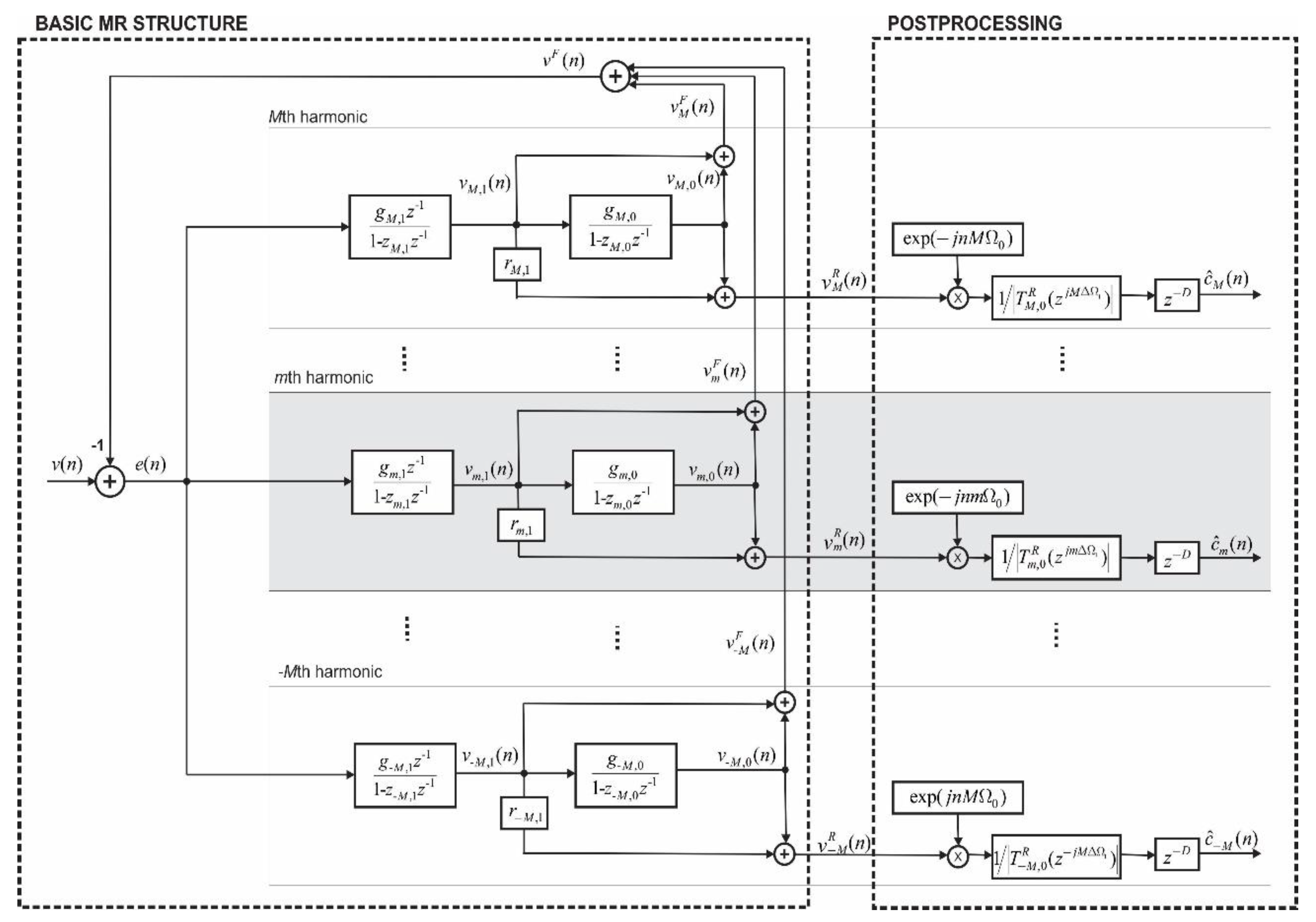
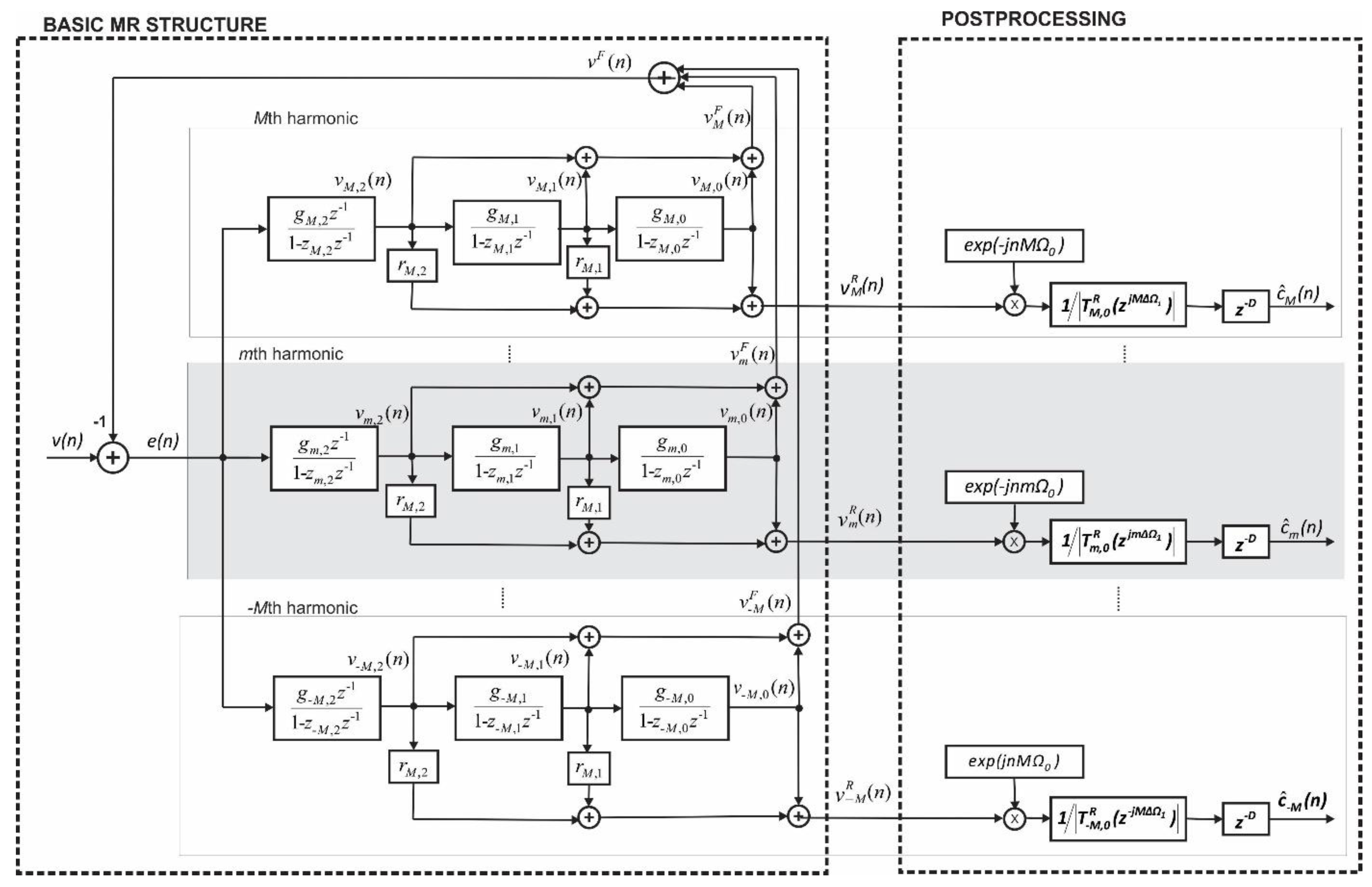
The block diagrams of the second-order and the third-order MR-based harmonic analyzers are shown in Figure 1 and Figure 2, respectively.

The cascade in the m-th channel consists of two (for $K=1$) or three (for $K=2$) resonators which poles are distributed closely on the unit circle around the pole of the mth harmonic frequency. In case of the true MR-based harmonic analyzer, all poles in the cascade are identical, i.e.:

$$z_{m,0}=z_{m,1}=\cdots =z_{m,K}=z_m=\exp \left(jm{\mathsf{\Omega }}_0\right)$$

(1)

where $m=-M,\dots ,0,\dots ,M$, $f_S$ is a sampling rate, and ${\mathsf{\Omega }}_0=2\pi f_0/f_S$ is a normalized angular frequency of the basic component.

To the resonators in the cascade are assigned corresponding complex gains $g_{m,k}$, $m=-M,\dots ,0,\dots ,M$, $k=0,\cdots ,K$.

Input signal is represented as follows:

$$v(n)={\displaystyle \sum _{m=-M}^M{v}_m(n)=}{\displaystyle \sum _{m=-M}^M{V}_m(n)\exp (jnm{\mathsf{\Omega }}_1)}$$

(2)

Outputs of the resonators are:

$$v_{m,k}(n)=c_{m,k}(n)\exp (jnm{\Omega }_1)$$

(3)

$m=-M,\dots ,0,\dots ,M$, $k=0,\cdots ,K$. The output signal $v_{m,k}(n)$ consists of the harmonic phasor complex envelope $c_{m,k}(n)$ and constantly rotating vector $\exp (jnm{\Omega }_1)$. Further, we suppose:

$$c_{m,k}(n)=a_{m,k}(n)\exp (j{\phi }_{m,k}(n))$$

(4)

and:

$$\begin{gathered} v_m^R\left(n\right)=v_{m,0}\left(n\right)+{{\displaystyle \sum }}_{k=1}^K{r}_{m,k}{v}_{m,k}\left(n\right) \\ {c}_m^R\left(n\right)=c_{m,0}\left(n\right)+{{\displaystyle \sum }}_{k=1}^K{r}_{m,k}{c}_{m,k}\left(n\right) \end{gathered}$$

(5)

The overall system orders are $\left(K+1\right)N$, $N=2M+1$ where $M{\mathsf{\Omega }}_0<\pi$.

2.1. K = 1. Type (The Second-Order) Harmonic Analyzer

In case of the dead-beat (all zero) observer, the transfer function assigned to the differentiators of the harmonic component $m$, for $K=1$, is as follows:

$$T_{m,0}\left(z\right)=\frac{V_{m,0}\left(z\right)}{V\left(z\right)}=\frac{g_{m,0}^{\prime }z{P}_m\left(z\right)}{z^{2N}}$$

(6)

$$T_{m,1}\left(z\right)=\frac{V_{m,1}\left(z\right)}{V\left(z\right)}=\frac{g_{m,1}^{\prime }\left(z-z_{m,0}\right)P_m\left(z\right)}{z^{2N}}$$

(7)

where:

$$P_m\left(z\right)={{\displaystyle \prod }}_{\begin{array}{c}i=-M\\ i\ne m\end{array}}^M\left(z-z_{i,0}\right)\left(z-z_{i,1}\right),$$

(8)

$z_i=\exp \left(j{\mathsf{\Omega }}_i\right)$, ${\mathsf{\Omega }}_i=i{\mathsf{\Omega }}_0,$ and:

$$g_{m,0}^{\prime }=g_{m,0}{g}_{m,1},g_{m,1}^{\prime }=g_{m,1}$$

(9)

In [59,60], closed-form solutions for gains ${\dot{g}}_{m,k}$, $k=0\dots K$, for true and quasi MRs, respectively, are given (see Appendix A).

In order to modify the dynamic properties, instead of $T_{m,0}\left(z\right)$ the linear combination of the differentiators can be used [61]:

$$T_{m,0}^R\left(z\right)=T_{m,0}\left(z\right)+r_{m,1}{T}_{m,1}\left(z\right)$$

(10)

In case of the dead-beat (all zero) observer, the transfer function $T_{m,0}\left(z\right)$ can be written as follows:

$$T_{m,0}\left(z\right)=z^{-D}{\acute{T}}_{m,0}\left(z\right)=z^{-D}\left[{\acute{T}}_{m,0}\left(z\right)+r_{m,1}{\acute{T}}_{m,1}\left(z\right)\right]$$

(11)

where:

$${\acute{T}}_{m,0}\left(z\right)=\frac{g_{m,0}^{\prime }z{P}_m\left(z\right)}{z^{2N-D}}$$

(12)

$${\acute{T}}_{m,1}\left(z\right)=\frac{g_{m,1}^{\prime }\left(z-z_{m,0}\right)P_m\left(z\right)}{z^{2N-D}}$$

(13)

It follows:

$$T_{m,0}^R\left(z\right)=z^{-D}{\acute{T}}_{m,0}^R\left(z\right)=z^{-D}\frac{Q_m\left(z\right)P_m\left(z\right)}{z^{2N-D}}$$

(14)

where:

$$Q_m\left(z\right)=g_{m,0}^{\prime }z+r_{m,1}{g}_{m,1}^{\prime }\left(z-z_m\right)$$

(15)

is a first-order compensation filter:

$${\acute{T}}_{m,0}^R\left(z\right)=\frac{Q_m\left(z\right)P_m\left(z\right)}{z^{2N-D}}$$

(16)

From the condition ${d{\acute{T}}_{m,0}^R\left(z\right)/dz|}_{z=z_m}=0$, it follows that [61]:

$$r_{m,1}=-g_{m,0}\left[1+\frac{z_m{\mathsf{\Psi }}_m\left(z_m\right)}{P_m\left(z_m\right)}\right]$$

(17)

See Appendix B. ${\acute{T}}_{m,0}^R\left(z\right)$ is noncausal and cannot be implemented real-time. A real-time implementation would require calculation $D$ samples cycle before the latest allowed sampling point. However, it can be implemented postpone at least $D$ samples delayed. Thus, measurement time stamp is defined by $D$. These $D$ samples are part of the latency. Another part of the latency is processing and communication time.

2.2. K = 2. Type (The Third-Order) Harmonic Analyzer

In case of the dead-beat (all zero) observer, the transfer function assigned to the differentiator of the harmonic component $m$, for $K=2$, is as follows:

$$T_{m,0}\left(z\right)=\frac{V_{m,0}\left(z\right)}{V\left(z\right)}=\frac{g_{m,0}^{\prime }{z}^2{P}_m\left(z\right)}{z^{3N}}$$

(18)

$$T_{m,1}\left(z\right)=\frac{V_{m,1}\left(z\right)}{V\left(z\right)}=\frac{g_{m,1}^{\prime }z\left(z-z_{m,0}\right)P_m\left(z\right)}{z^{3N}}$$

(19)

$$T_{m,2}\left(z\right)=\frac{V_{m,2}\left(z\right)}{V\left(z\right)}=\frac{g_{m,2}^{\prime }\left(z-z_{m,0}\right)\left(z-z_{m,1}\right)P_m\left(z\right)}{z^{3N}}$$

(20)

where $P_m\left(z\right)={{\displaystyle \prod }}_{\begin{array}{c}i=-M\\ i\ne m\end{array}}^M\left(z-z_{i,0}\right)\left(z-z_{i,1}\right)\left(z-z_{i,2}\right),$ $z_i=\exp \left(j{\mathsf{\Omega }}_i\right)$, ${\mathsf{\Omega }}_i=i{\mathsf{\Omega }}_0$ and:

$$g_{m,0}^{\prime }=g_{m,0}{g}_{m,1}{g}_{m,2},g_{m,1}^{\prime }=g_{m,1}{g}_{m,2},g_{m,2}^{\prime }=g_{m,2}$$

(21)

In [59,60], closed-form solutions for gains ${\dot{g}}_{m,k}$, $k=0\dots K$, for true and quasi MRs, respectively, are given (see Appendix C).

The linear combination of the differentiators has the following form:

$$T_{m,0}^R\left(z\right)=T_{m,0}\left(z\right)+r_{m,1}{T}_{m,1}\left(z\right)+r_{m,2}{T}_{m,2}\left(z\right)$$

(22)

Further, it is:

$$T_{m,0}^R\left(z\right)=z^{-D}{\acute{T}}_{m,0}^R\left(z\right)=z^{-D}\frac{Q_m\left(z\right)P_m\left(z\right)}{z^{3N-D}}$$

(23)

$$Q_m\left(z\right)=g_{m,0}^{\prime }{z}^2+r_{m,1}{g}_{m,1}^{\prime }z\left(z-z_{m,0}\right)+r_{m,2}{g}_{m,2}^{\prime }\left(z-z_{m,0}\right)\left(z-z_{m,1}\right)$$

(24)

From ${d{\acute{T}}_{m,0}^R\left(z\right)/dz|}_{z=z_m}=0$, it follows that [61]:

$$r_{m,1}=-g_{m,0}\left[2+\frac{z_m{\mathsf{\Psi }}_m\left(z_m\right)}{P_m\left(z_m\right)}\right]$$

(25)

Further, from the condition ${d^2{\acute{T}}_{m,0}^R\left(z\right)/d{z}^2|}_{z=z_m}=0$, it follows that [61]:

$$r_{m,2}=-g_{m,1}\left[z_m\frac{2\left(2g_{m,0}+r_{m,1}\right){\mathsf{\Psi }}_m\left(z_m\right)+g_{m,0}{z}_m{\mathsf{\Phi }}_m\left(z_m\right)}{2P_m\left(z_m\right)}+g_{m,0}+r_{m,1}\right]$$

(26)

See Appendix D.

2.3. Frequency Responses of the Selected Characteristic Cases

Table 1. Coefficients for Considered Values of D for $K=1$.

Estimator type	$\mathit{D}$	${\mathit{r}}_{\mathit{m},1}$
$D_{1,1}$	16	0.0000
$D_{1,2}$	20	−0.2500

and

Table 2. Coefficients for Considered Values of D for $K=2$.

Estimator type	$\mathit{D}$	${\mathit{r}}_{\mathit{m},1}$	${\mathit{r}}_{\mathit{m},2}$
$D_{2,1}$	24	−0.0213	−0.1250

summarize values of the coefficients applied for the second-order ($K=1$) estimator for $D_{1,1}=16$, and $D_{1,2}=20$, and the third-order ($K=2$) estimator, for $D_{2,1}=24$, with $f_1=50\mathrm{Hz}$ and $f_S=800\mathrm{Hz}$ ($N=16$). It should be mentioned that for the coherent sampling conditions, parameters determined by Equations (17), (25) and (26) are equal for all harmonics [61].

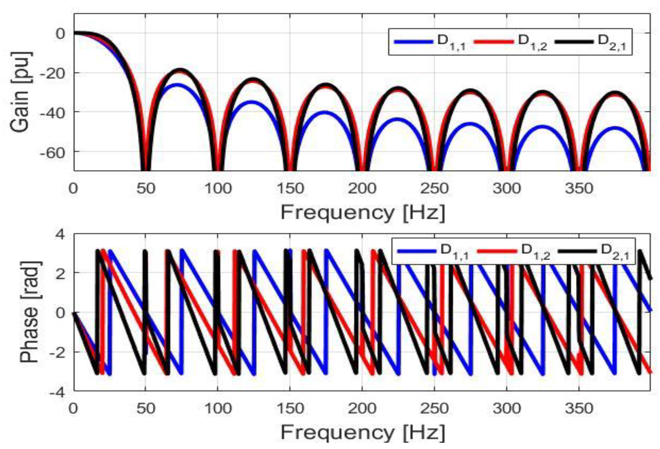
Figure 3 shows the frequency responses of the transfer function of DC component $T_{m,0}^R\left(z\right)$ in $K=1$ and $K=2$ cases, for the values of $D$ selected in the Table 1 and Table 2. The frequency responses for DC component ($m=0$) are depicted only. Frequency responses for other harmonics show the same performances.

The flatness of the amplitude frequency responses around the harmonic frequency is wider for $K=2$. In addition to that, multiple zeros ensure zero-flat gains at the harmonics but at cost of the increase of sidelobe levels with the decrease of the delay $D$. At the same time, the group delay rises with the increase of $K$.

For $K=1$ and $D_{1,1}=16$ the amplitude frequency response shows narrow flatness in the passband. The frequency responses in this case corresponds to the frequency response of a two-cycle triangular weighted FIR reference filter [6] (Appendix D) suggested by the IEC/IEEE Standard. The wider flatness exists for $D_{1,2}=20$.

3. Postprocessing

The second part of the structure deals with the postprocessing and includes demodulation of the resonators output signals. Note that the postprocessing can be carried out for selected harmonics, e.g., the fundamental component and significant harmonics.

3.1. Harmonic Phasor Estimation

A harmonic signal is present as an output of the resonators cascade as:

$$v_m^R\left(n\right)=v_{m,0}\left(n\right)+{{\displaystyle \sum }}_{k=1}^K{r}_{m,k}{v}_{m,k}\left(n\right)=c_m^R\left(n\right)\exp \left(jnm{\mathsf{\Omega }}_1\right)$$

(27)

From this signal, an estimation of the phasor $c_m\left(n\right)$ it can be obtained by demodulation with:

$${\widehat{c}}_m\left(n\right)=c_m^R\left(n\right)\exp \left(jnm{\mathsf{\Omega }}_1\right)\exp \left(-jnm{\mathsf{\Omega }}_0\right)=c_m^R\left(n\right)e^{i{\phi }_m\left(n\right)}$$

(28)

where ${\phi }_m\left(n\right)=nm\mathsf{\Delta }{\mathsf{\Omega }}_1$, $\mathsf{\Delta }{\mathsf{\Omega }}_1={\mathsf{\Omega }}_1-{\mathsf{\Omega }}_0$.

Frequency deviation from the nominal one creates errors in magnitude and phase spectrum responses and have drooping passband gains. It changes the magnitude and phase of the components of the signal. To eliminate the side effect of the proposed filter, multiplication (division) with correction factors is necessary. In addition to that, the time stamp of the measurement allocation for $D$ steps is implemented by time-shifting operation:

$${\widehat{c}}_m\left(n-D\right)=c_m^R\left(n\right)/\left|T_{m,0}^R\left(z^{jm\mathsf{\Delta }{\mathsf{\Omega }}_1}\right)\right|$$

(29)

The correction factors can be calculated offline and conveniently retrieved online. This way, the computational burden can be reduced.

3.2. Frequency and ROCOF Estimation

Estimation of the frequency and ROCOF is convenient to consider separately since it depends on the chosen algorithm. It can be considered as a whole together with the phasor measurement, can be a separate postprocessing step following the phasor estimation or, more generally, it can be a completely different estimation unit [1].

The frequency and ROCOF are given by the first- and second-order time-derivative of the estimated phase angle, respectively, as follows:

$$\widehat{f}=f_0+\frac{1}{2\pi }\frac{d\phi }{dt}$$

(30)

$$\widehat{ROCOF}=\frac{d\widehat{f}}{dt}=\frac{1}{2\pi }\frac{d^2\phi }{d^{2}t}$$

(31)

The MR-based filter structure has an advantage that the fundamental and harmonic phasors derivatives involve the fundamental and harmonic frequencies and their ROCOFs and, thus, they can be estimated simultaneously. The first phasor derivative $c_{1,1}\left(n\right)$ and the second phasor derivative $c_{1,2}\left(n\right)$ can be used for frequency and ROCOF estimation. For both K = 1 and K = 2, the frequency deviation can be calculated as follows:

$$\widehat{f}-f_0\cong \frac{\mathrm{Im}\left\{c_{1,1}\left(n\right)c_{1,0}^{*}\left(n\right)\right\}}{2\pi {\left|c_{1,0}\left(n\right)\right|}^2}{f}_0=\frac{\mathrm{Im}\left\{v_{1,1}\left(n\right)v_{1,0}^{*}\left(n\right)\right\}}{2\pi {\left|v_{1,0}\left(n\right)\right|}^2}{f}_0$$

(32)

where * denotes the conjugate operation, and $\widehat{}$ estimation.

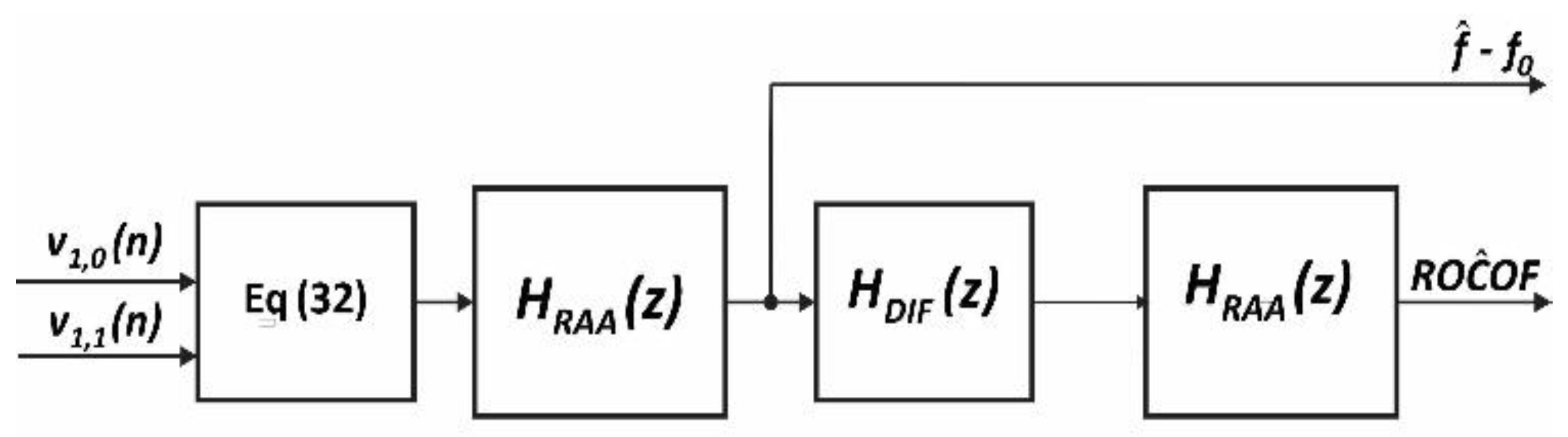
The ROCOF can also be estimated using the estimates of the phasor derivatives. In this case, the presence of the wideband noise decreases the accuracy of the method significantly [25]. In this article the FIR differentiators of order seven is used. Output of the differentiators are further filtered by the following recursive averaging algorithm (RAA):

$$H_{RAA}(N_{RAA},z)=\frac{1}{N_{RAA}}\frac{\left(1-z^{-N_{RAA}}\right)}{1-z^{-1}}$$

(33)

The window length $N_{RAA}$ has to be selected in compliance with the expected variation range and bandwidth of ROCOF. Figure 4 shows block diagram of the frequency and the ROCOF estimator. $N_{RAA}$ for RAA after differentiators for ROCOF estimation are chosen to be equal 16. RAA with $N_{RAA}=8$ after the block for frequency estimation is used only for $K=1$.

The performances of the frequency and ROCOF estimators strongly depends on the filters (both inherent in the basic resonator structure and the filters for the postprocessing). Consequently, for low ROCOF errors, longer latencies are needed. For low latency, larger ROCOF ripple and errors are expected.

4. Simulation Results

The frequency response approach presented in the previous section is useful to clarify the harmonic phasor estimates behavior, particularly when the input signal contains disturbances which are not involved into the signal model such as noise and/or interharmonic components. In this section, extensive simulation tests are performed to evaluate and compare the performance of the selected cases in accordance with the IEC/IEEE Standard specifications. The IEC/IEEE Standard specifies the compliance requirements for steady state and dynamic conditions. The estimates for the second-order ($K=1$) estimator for $D_{1,1}=16$, $D_{1,2}=20$, and the third-order ($K=2$) estimator, for $D_{2,1}=24$, and with $f_1=50\mathrm{Hz}$ and $f_S=800 \mathrm{Hz}$ ($N=16$), are shown in Figure 5, Figure 6, Figure 7, Figure 8, Figure 9 and Figure 10.

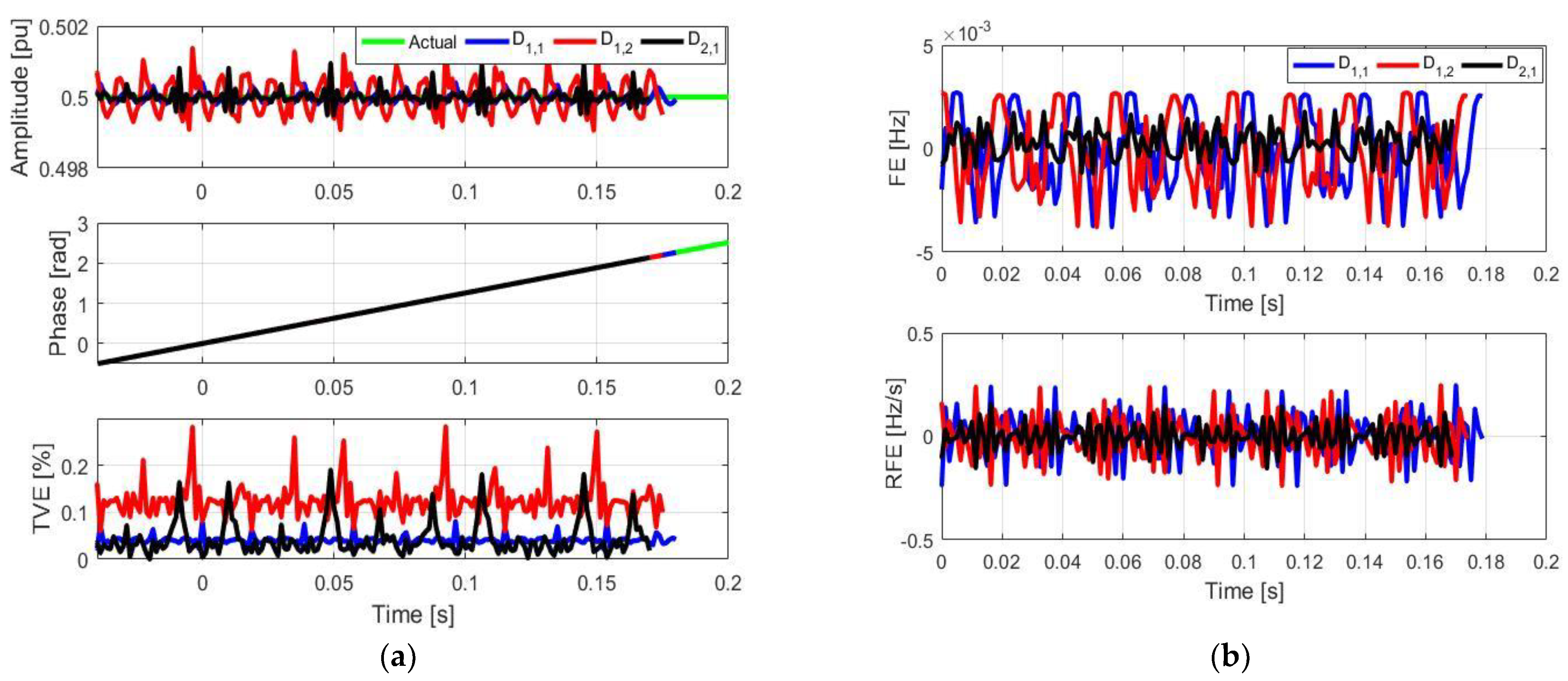
4.1. Steady-State Characteristic

The compliance of the MR algorithm has been proofed through reproducing test conditions in different Class P testing conditions specified in the IEC/IEEE Standard 60255-118-1:2018 [6] in case the waveform is affected by both off-nominal frequency deviations within ± 2 Hz and steady-state harmonics (up to seventh), taken simultaneously at a time, each of amplitude equal to 1%. The estimates for the fundamental component are depicted only since the waveforms of estimates for harmonic phasors have similar shapes. Figure 5 shows estimates of the TVE, FE and ROCOF for the fundamental component for $K=1$ (for $D_{1,1} \mathrm{and} D_{1,2}$) and $K=2$ (for $D_{2,1}$) type estimators with $f_1=52 \mathrm{Hz}$ and $f_S=800 \mathrm{Hz}$. The estimation results comply with the frequency responses shown in Figure 4. $T_{m,0}^R\left(z\right)$ for $D_{1,2}$ and $D_{2,1}$ provides larger TVE due to higher sidelobes. Errors obtained by $D_{1,1}$ are smaller, due to the lower level of sidelobes and narrower passband.

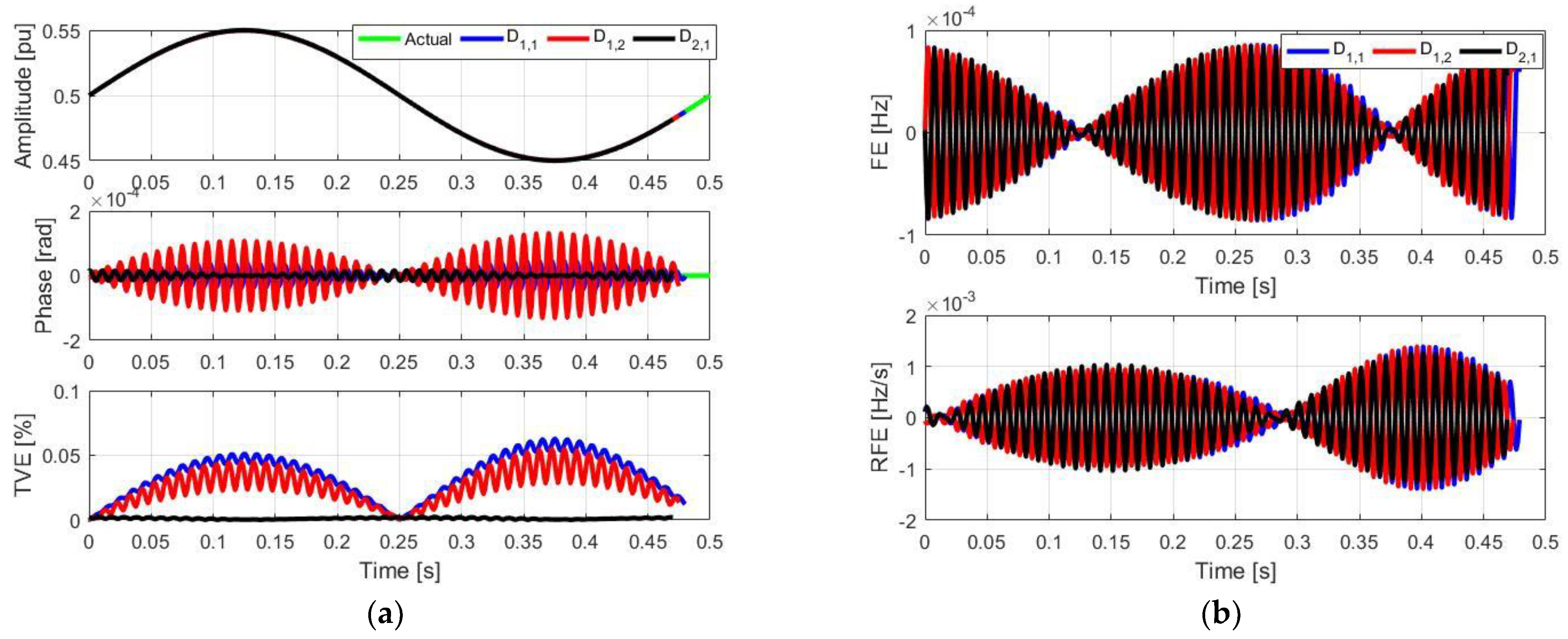
4.2. Amplitude and Phase Modulated Signals

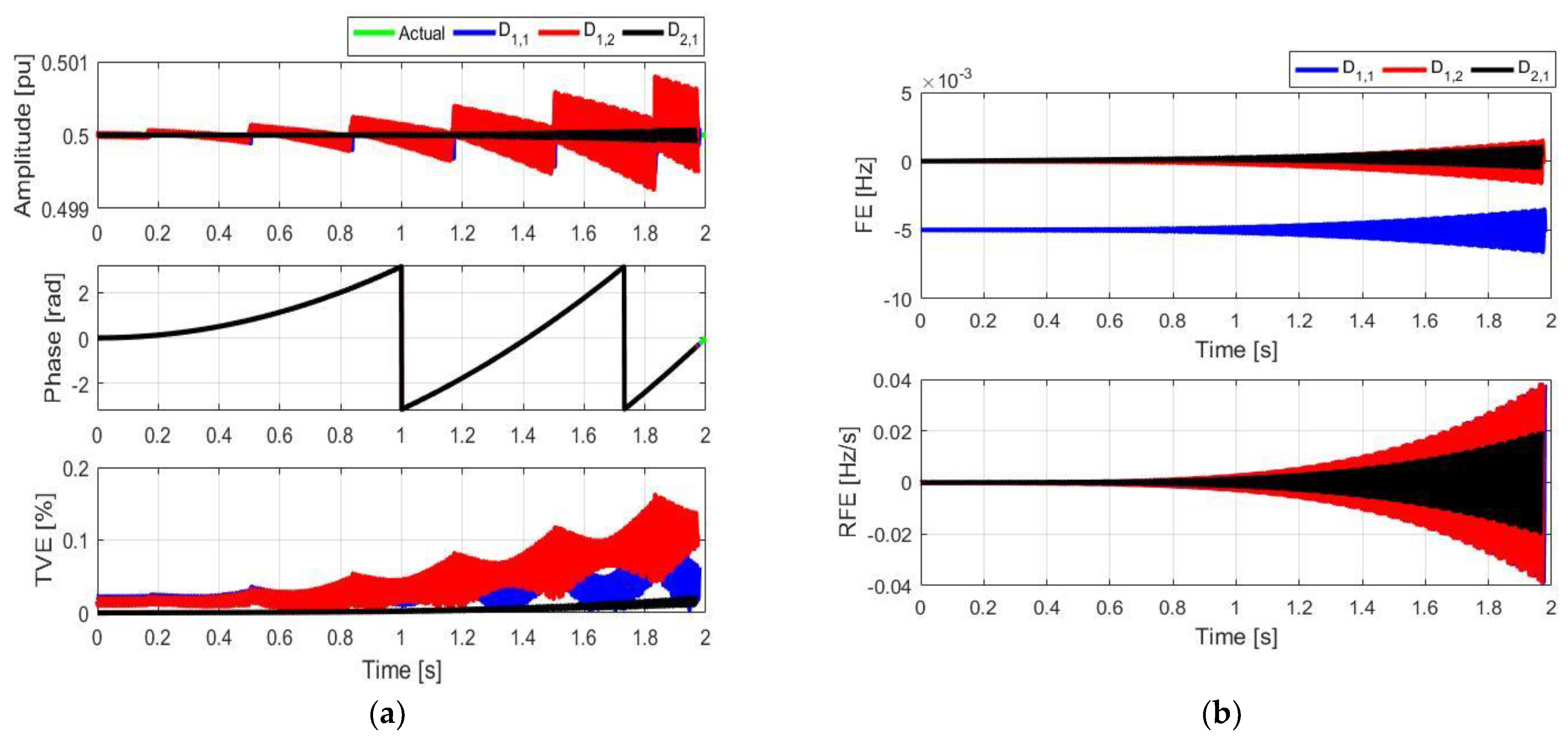
Tests with the amplitude and phase modulated signals are applied to determine PMU measurement bandwidth. The test signal defined by the standard is as follows:

$$s\left(t\right)=X_m\left[1+k_x\cos \left(2\pi f_{m}t\right)\right]\cos \left[2\pi f_{1}t+k_a\cos \left(2\pi f_{m}t-\pi \right)\right]$$

(34)

where $X_m$ is the fundamental component amplitude, the amplitude and phase modulation depths are denoted as $k_{x }$ and $k_a$, respectively, and $f_m$ is the modulating signal frequency. Values of modulated signals are chosen in line with the suggestion of the PMU IEC/IEEE Standard 60255-118-1:2018-2011 [6]. The amplitude and phase angle modulation depths of $k_x=0.1$ p.u. and $k_a=0.1 \mathrm{rad}$ are considered. For P class test, the maximum modulation frequency is $f_m=2\mathrm{Hz}$. The fundamental frequency is constant during time and equals $50 \mathrm{Hz}$. $X_m=1 \left(\mathrm{p}.\mathrm{u}.\right)$.

The influence of a modulation of the sinusoidal amplitude of magnitude amounting 10% of the fundamental one and the modulation frequency equal to 2 Hz is shown in Figure 6. In Figure 6, it is notable that the TVE obtained by $D_{2,1}=24$ is very low (smaller than 0.002%) and negligible in relation to the standards limit of 3%. The FE and RFE are similar in all cases and their maxima are 0.1 mHz and 1.5 mHz/s, respectively. It is notable that the limits of 30 mHz for FE and 600 mHz/s allowed by the standard are much higher.

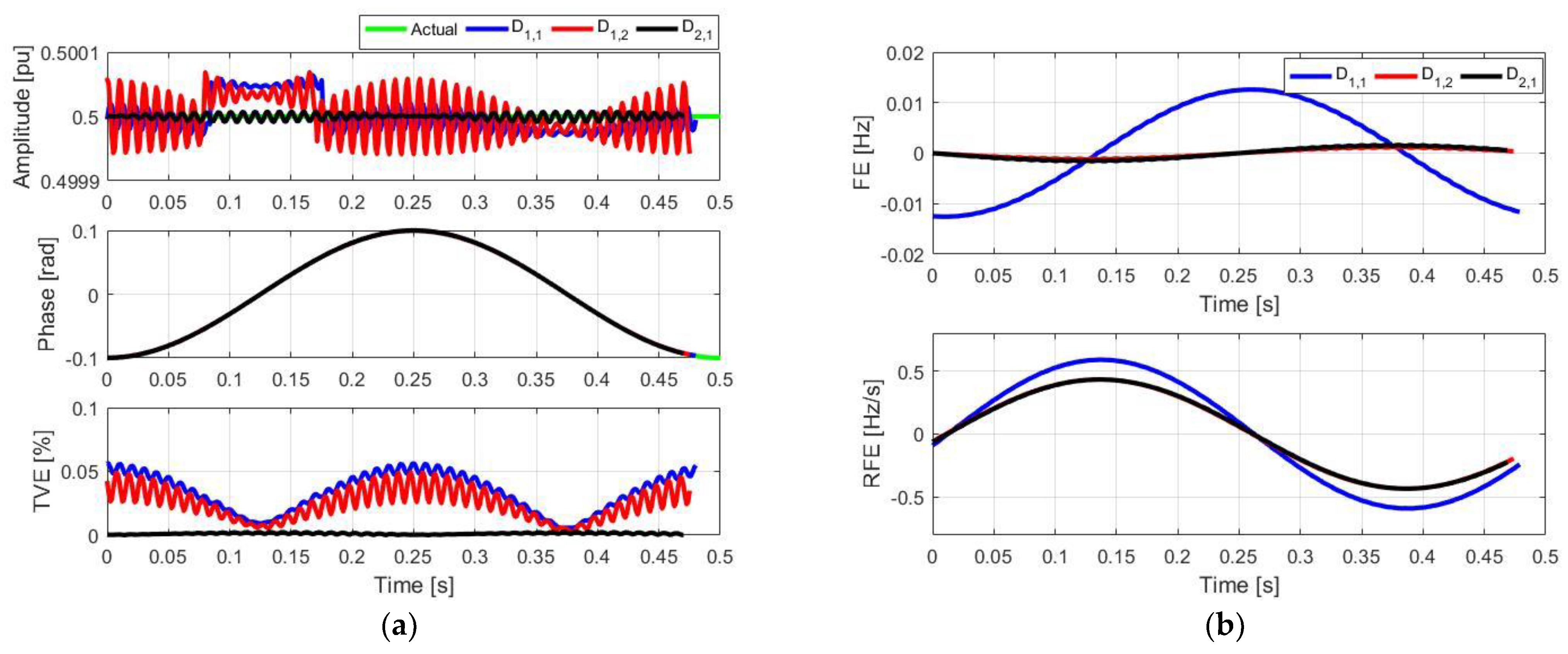
Secondly, the influence of a sinusoidal phase modulation of amplitude equal to 0.1 rad and the modulation frequency amounting $f_m=2 \mathrm{Hz}$ is illustrated in Figure 7. Figure 7 shows that all of three cases satisfy the standards requirements. The algorithm satisfies the measurement bandwidth TVE compliance up to modulation frequency of $2 \mathrm{Hz}$ since the maximum value of the determined TVE is much less than 3%, but again the case $K=2$ for $D_{2,1}=24$ outperforms both $K=1$ cases. From Figure 7b it is noticeable that $K=2$ for $D_{2,1}=24$ and $K=1$ for $D_{1,2}=20$ provide smaller FEs than $K=1$ for $D_{1,1}=16$, thanks to the wider passband. It should be noted that the performances of the frequency and ROCOF estimators strongly depends on the postprocessing filters. A higher order of RAA influences larger FE and RFE and vice versa.

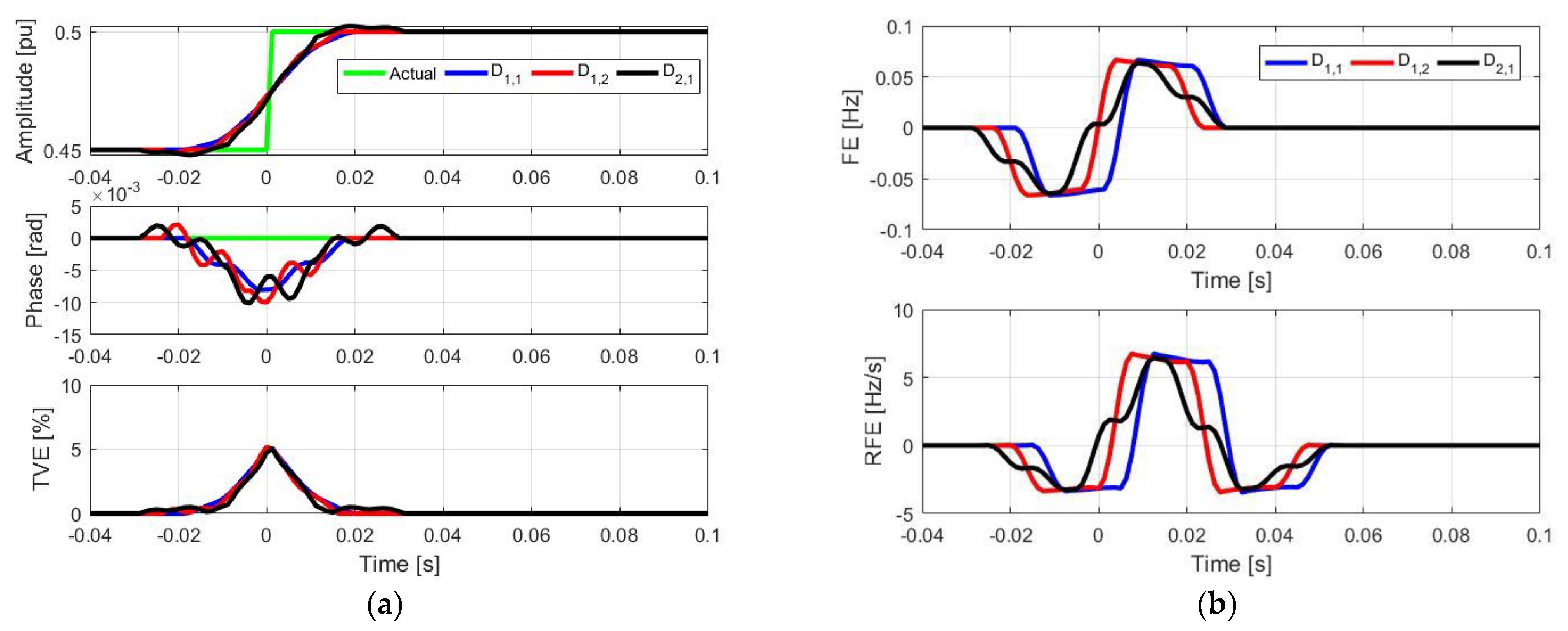
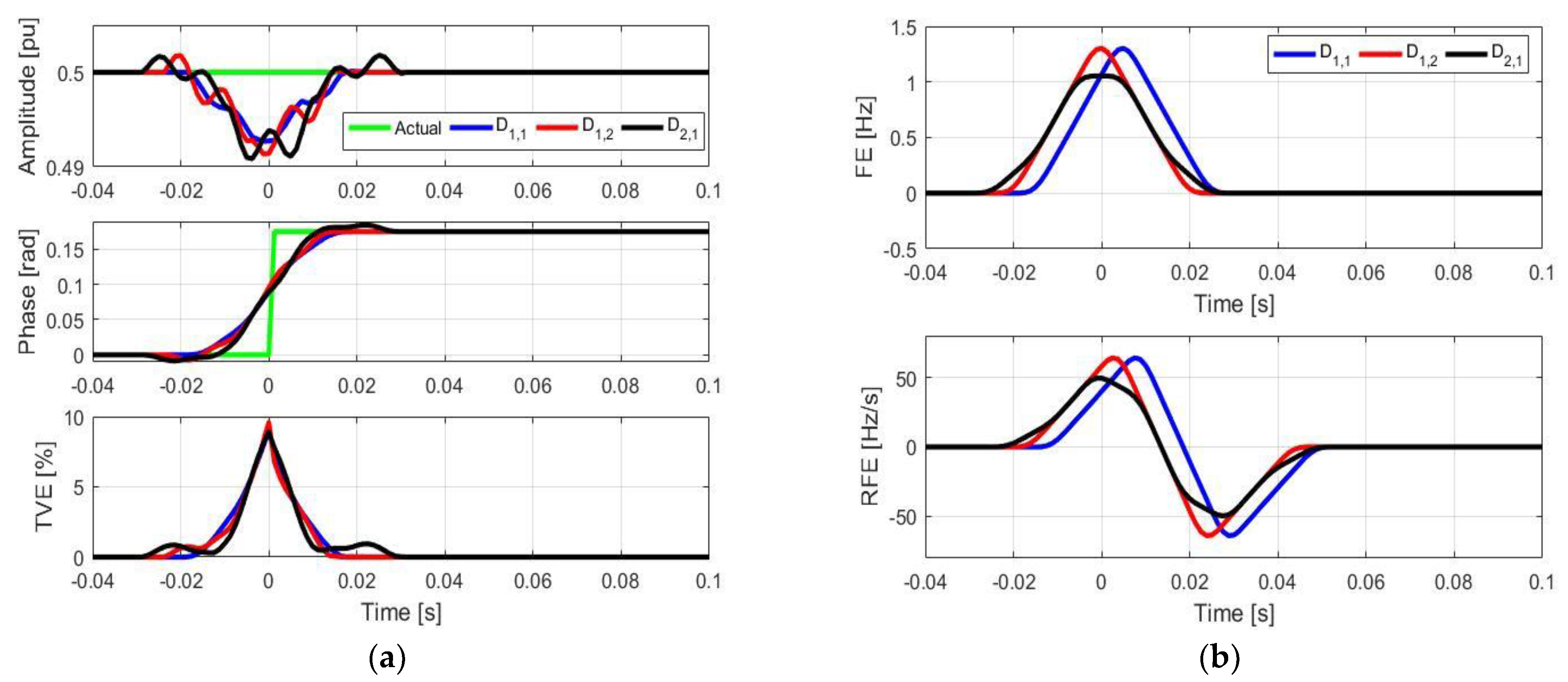
4.3. Amplitude and Phase Step Signals

In these tests, signals with the phase angle shift equal 10° and the step change from 0.9 to 1 p.u. of the amplitude in the fundamental component, respectively, are fed to the estimator. The test signal defined by the standard is as follows:

$$s\left(t\right)=X_m\left[1+k_x\cos \left(2\pi f_{m}t\right)\right]\cos \left[2\pi f_{1}t+k_a\cos \left(2\pi f_{m}t-\pi \right)\right]$$

(35)

where $u\left(t\right)$ is the unit step function and $t_S$ is an instant time of the step. The amplitude step is given with $k_x=0.1$ and phase step with $k_a=\pi /18$ (10° phase angle step). The fundamental frequency is constant during time and equals 50 Hz. Figure 8 illustrates a convergence in the amplitude shift (with $k_x=0.1$ and $k_a=0$). It is possible to note overshoots of about 5% in case of $K=1$, for $D_{1,2}=20$, and $K=2$ for $D_{2,1}=24$. This overshoot is maximally allowed overshoots by the standard for P-Class PMUs.

Figure 9 shows the time responses corresponding to the phase shift (with $k_x=0$ and $k_a=\pi /18$). Again, overshoots are about 5% in case of $K=1$, for $D_{1,2}=20$, and $K=2$ for $D_{2,1}=24$. This overshoot is maximally allowed overshoots by the standard for P-Class PMUs.

A maximum allowed frequency response time for both amplitude and phase steps according the standard is 90 ms. It is notable that actual frequency response times are a half of that. Obtained ROCOF response times are about 80 ms, while maximum allowed ones per standard are 120 ms. It is important to note that the phase steps are a major challenge for ROCOF measurements.

4.4. Frequency Ramp

In the following frequency ramp test, the frequency of a voltage signal is ramped up keeping the amplitude of the signal constant. For simulation purposes, $v\left(t\right)=\cos \left(2\pi f_{0}t+\pi R_f{t}^2\right)$ is used, where $R_f=1$ $\mathrm{Hz}/\mathrm{s}$ is the rate of change of the fundamental frequency. The range of the fundamental frequency variation is from 50 to 52 Hz. In Figure 10, the corresponding obtained results are given. For the amplitude and TVE calculation, a correction of the amplitude of the signal is applied according an actual frequency estimation. Since the gains of the frequency responses are previously calculated with a resolution of $1/3$ Hz, small discontinuities are present. Again, the maximum TVEs, FEs, and RFEs obtained with the proposed algorithm are smaller for $D_{2,1}$.

The standard prescribes the TVE, FE, and RFE limits for the P-class PMUs as 1%, 0.01 Hz, and 0.4 Hz/s, respectively. The maximum achieved FE and RFE are smaller than the limits of the standard. It should be noted that for low ROCOF errors, higher orders of RAA filters are needed causing longer latencies. For low latency, large ROCOF ripple and errors are expected.

5. Conclusions

In this article, it is shown that recursive MR-based estimation technique exhibiting MF frequency responses can be efficiently used for implementation of P-Class Compliant PMUs in accordance with IEC/IEEE Standard 60255-118-1:2018. The proposed algorithm is very convenient for a real-time digital implementation due to its parallel structure and the recursive computation. Computer simulation tests have been performed under different conditions, considering the presence of up to 64 harmonics, presenting algorithms performances and compatibility with 60255-118-1:2018. The proposed method for $K=1$ and $K=2$ confirmed to be compliant with IEC/IEEE Standard 60255-118-1:2018 test specification for P-class, for both the fundamental component together with significant low-order harmonic phasors.

Due to its wider passband, $K=2$ case provides better dynamics performances, while $K=1$ for $D_{1,1}$ shown better accuracy in steady state conditions. For $K=1$ for $D_{1,2}$ obtained performances are between these two.

References

- Monti, A.; Muscas, C.; Ponci, F. Phasor Measurement Units and Wide Area Monitoring Systems: From the Sensors to the System; Elsevier Inc.: Amsterdam, The Netherlands, 2016. [Google Scholar] [CrossRef]
- Castello, P.; Ferrari, P.; Flammini, A.; Muscas, C.; Rinaldi, S. A New IED with PMU Functionalities for Electrical Substations. IEEE Trans. Instrum. Meas. 2013, 62, 3209–3217. [Google Scholar] [CrossRef]
- Jain, A.; Samantaray, S.R.; Geoffroy, L.; Kamwa, I. Synchrophasors Data Analytics Framework for Power Grid Control and Dynamic Stability Monitoring. Eng. Technol. Ref. 2016, 1. [Google Scholar] [CrossRef]
- Atalik, T.; Çadirci, I.; Demirci, T.; Ermis, M.; Inan, T.; Kalaycioglu, A.S.; Salor, Ö. Multipurpose Platform for Power System Monitoring and Analysis with Sample Grid Applications. IEEE Trans. Instrum. Meas. 2014, 63, 566–582. [Google Scholar] [CrossRef]
- Laverty, D.M.; Best, R.J.; Brogan, P.; Al Khatib, I.; Vanfretti, L.; Morrow, D.J. The OpenPMU Platform for Open-Source Phasor Measurements. IEEE Trans. Instrum. Meas. 2013, 62, 701–709. [Google Scholar] [CrossRef] [Green Version]
- IEC/IEEE Standard 60255-118-1:2018 Part 118-1: Synchrophasor Measurements for Power Systems; IEEE STD23444; International Electrotechnical Commission: Geneva, Switzerland, 2018; ISBN 978-1-5044-5361-5. [CrossRef]
- IEEE Std C37.118.1-2011, IEEE Standard for Synchrophasor Measurements for Power Systems; IEEE STD97167; IEEE Inc.: New York, NY, USA, 2011; ISBN 978-0-7381-6811-1. [CrossRef]
- IEEE Std C37.118.1a-2014, IEEE Standard for Synchrophasor Measurements for Power Systems—Amendment 1: Modification of Selected Performance Requirements; IEEE STD98573; IEEE Inc.: New York, NY, USA, 2014; ISBN 978-0-7381-8978-9. [CrossRef]
- Martin, K.E.; Goldstein, A.R.; Adamiak, M.G.; Antonova, G.; Begovic, M.; Benmouyal, G.; Brunello, G.; Dickerson, B.; Hu, Y.; Jalali, M.; et al. Synchrophasor Measurements under the IEEE Standard C37.118.1-2011 with Amendment C37.118.1a. IEEE Trans. Power Deliv. 2015, 30, 1514–1522. [Google Scholar] [CrossRef]
- Premerlani, W.; Kasztenny, B.; Adamiak, M. Development and Implementation of a Synchrophasor Estimator Capable of Measurements under Dynamic Conditions. IEEE Trans. Power Deliv. 2007, 23, 109–123. [Google Scholar] [CrossRef]
- Phadke, A.G.; Kasztenny, B. Synchronized Phasor and Frequency Measurement under Transient Conditions. IEEE Trans. Power Deliv. 2008, 24, 89–95. [Google Scholar] [CrossRef]
- Mai, R.K.; He, Z.Y.; Fu, L.; Kirby, B.; Bo, Z.Q. A Dynamic Synchrophasor Estimation Algorithm for Online Application. IEEE Trans. Power Deliv. 2010, 25, 570–578. [Google Scholar] [CrossRef]
- Barchi, G.; MacIi, D.; Petri, D. Synchrophasor Estimators Accuracy: A Comparative Analysis. IEEE Trans. Instrum. Meas. 2013, 62, 963–973. [Google Scholar] [CrossRef]
- Belega, D.; MacIi, D.; Petri, D. Fast Synchrophasor Estimation by Means of Frequency-Domain and Time-Domain Algorithms. IEEE Trans. Instrum. Meas. 2013, 63, 388–401. [Google Scholar] [CrossRef]
- De Carvalho, J.R.; Duque, C.A.; Lima, M.A.A.; Coury, D.V.; Ribeiro, P.F. A Novel DFT-Based Method for Spectral Analysis under Time-Varying Frequency Conditions. Electr. Power Syst. Res. 2014, 108, 74–81. [Google Scholar] [CrossRef]
- Belega, D.; Dallet, D. Multifrequency Signal Analysis by Interpolated DFT Method with Maximum Sidelobe Decay Windows. Measurement 2009, 42, 420–426. [Google Scholar] [CrossRef]
- Belega, D.; Petri, D. Accuracy Analysis of the Multicycle Synchrophasor Estimator Provided by the Interpolated DFT Algorithm. IEEE Trans. Instrum. Meas. 2013, 62, 942–953. [Google Scholar] [CrossRef]
- Romano, P.; Paolone, M. Enhanced Interpolated-DFT for Synchrophasor Estimation in FPGAs: Theory, Implementation, and Validation of a PMU Prototype. IEEE Trans. Instrum. Meas. 2014, 63, 2824–2836. [Google Scholar] [CrossRef]
- Petri, D.; Fontanelli, D.; Macii, D. A Frequency-Domain Algorithm for Dynamic Synchrophasor and Frequency Estimation. IEEE Trans. Instrum. Meas. 2014, 63, 2330–2340. [Google Scholar] [CrossRef]
- Derviskadic, A.; Romano, P.; Paolone, M. Iterative-Interpolated DFT for Synchrophasor Estimation: A Single Algorithm for P-and M-Class Compliant PMUs. IEEE Trans. Instrum. Meas. 2017, 67, 547–558. [Google Scholar] [CrossRef] [Green Version]
- Tosato, P.; Macii, D.; Luiso, M.; Brunelli, D.; Gallo, D.; Landi, C. A Tuned Lightweight Estimation Algorithm for Low-Cost Phasor Measurement Units. IEEE Trans. Instrum. Meas. 2018, 67, 1047–1057. [Google Scholar] [CrossRef]
- Chakir, M.; Kamwa, I.; Le Huy, H. Extended C37.118.1 PMU Algorithms for Joint Tracking of Fundamental and Harmonic Phasors in Stressed Power Systems and Microgrids. IEEE Trans. Power Deliv. 2014, 29, 1465–1480. [Google Scholar] [CrossRef]
- Belega, D.; Petri, D. Accuracy of Synchrophasor Measurements Provided by the Sine-Fit Algorithms. In Proceedings of the 2012 IEEE International Energy Conference and Exhibition, ENERGYCON 2012, Florence, Italy, 9–12 September 2012; pp. 921–926. [Google Scholar] [CrossRef]
- Chen, L.; Zhao, W.; Wang, Q.; Wang, F.; Huang, S. Dynamic Harmonic Synchrophasor Estimator Based on Sinc Interpolation Functions. IEEE Trans. Instrum. Meas. 2018, 68, 3054–3065. [Google Scholar] [CrossRef]
- Chen, L.; Zhao, W.; Wang, F.; Huang, S. Harmonic Phasor Estimator for P-Class Phasor Measurement Units. IEEE Trans. Instrum. Meas. 2020, 69, 1556–1565. [Google Scholar] [CrossRef]
- Platas-Garza, M.A.; De La O Serna, J.A. Dynamic Harmonic Analysis through Taylor-Fourier Transform. IEEE Trans. Instrum. Meas. 2010, 60, 804–813. [Google Scholar] [CrossRef]
- Platas-Garza, M.A.; De La O Serna, J.A. Polynomial Implementation of the Taylor-Fourier Transform for Harmonic Analysis. IEEE Trans. Instrum. Meas. 2014, 63, 2846–2854. [Google Scholar] [CrossRef]
- Petrović, P.; Damljanović, N. Dynamic Phasors Estimation Based on Taylor-Fourier Expansion and Gram Matrix Representation. Math. Probl. Eng. 2018, 2018, 7613814. [Google Scholar] [CrossRef] [Green Version]
- Zecevic, Z.; Krstajic, B. Dynamic Harmonic Phasor Estimation by Adaptive Taylor-Based Bandpass Filter. IEEE Trans. Instrum. Meas. 2021, 70, 1–9. [Google Scholar] [CrossRef]
- De La O Serna, J.A.; Rodríguez-Maldonado, J. Instantaneous Oscillating Phasor Estimates with TaylorK-Kalman Filters. IEEE Trans. Power Syst. 2011, 26, 2336–2344. [Google Scholar] [CrossRef]
- De La O Serna, J.A.; Rodríguez-Maldonado, J. Taylor-Kalman-Fourier Filters for Instantaneous Oscillating Phasor and Harmonic Estimates. IEEE Trans. Instrum. Meas. 2012, 61, 941–951. [Google Scholar] [CrossRef]
- Liu, J.; Ni, F.; Pegoraro, P.A.; Ponci, F.; Monti, A.; Muscas, C. Fundamental and Harmonie Synchrophasors Estimation Using Modified Taylor-Kaiman Filter. In Proceedings of the 2012 IEEE International Workshop on Applied Measurements for Power Systems, AMPS 2012 Proceedings, Aachen, Germany, 26–28 September 2012; IEEE Inc.: New York, NY, USA, 2012; pp. 30–35. [Google Scholar] [CrossRef]
- Karimi-Ghartemani, M.; Ooi, B.T.; Bakhshai, A. Application of Enhanced Phase-Locked Loop System to the Computation of Synchrophasors. IEEE Trans. Power Deliv. 2010, 26, 22–32. [Google Scholar] [CrossRef]
- McNamara, D.M.; Ziarani, A.K.; Ortmeyer, T.H. A New Technique of Measurement of Nonstationary Harmonics. IEEE Trans. Power Deliv. 2006, 22, 387–395. [Google Scholar] [CrossRef]
- De La O Serna, J.A. Synchrophasor Measurement with Polynomial Phase-Locked-Loop Taylor-Fourier Filters. IEEE Trans. Instrum. Meas. 2015, 64, 328–337. [Google Scholar] [CrossRef]
- Messina, F.; Marchi, P.; Vega, L.R.; Galarza, C.G.; Laiz, H. A Novel Modular Positive-Sequence Synchrophasor Estimation Algorithm for PMUs. IEEE Trans. Instrum. Meas. 2016, 66, 1164–1175. [Google Scholar] [CrossRef]
- de la O Serna, J.A. Dynamic Phasor Estimates for Power System Oscillations. IEEE Trans. Instrum. Meas. 2007, 56, 1648–1657. [Google Scholar] [CrossRef]
- Badrkhani Ajaei, F.; Sanaye-Pasand, M.; Davarpanah, M.; Rezaei-Zare, A.; Iravani, R. Mitigating the Impacts of CCVT Subsidence Transients on the Distance Relay. IEEE Trans. Power Deliv. 2012, 27, 497–505. [Google Scholar] [CrossRef]
- Das, S.; Sidhu, T. A Simple Synchrophasor Estimation Algorithm Considering IEEE Standard C37.118.1-2011 and Protection Requirements. IEEE Trans. Instrum. Meas. 2013, 62, 2704–2715. [Google Scholar] [CrossRef]
- Platas-Garza, M.A.; De La O Serna, J.A. Dynamic Phasor and Frequency Estimates through Maximally Flat Differentiators. IEEE Trans. Instrum. Meas. 2009, 59, 1803–1811. [Google Scholar] [CrossRef]
- Giarnetti, S.; Leccese, F.; Caciotta, M. Non Recursive Multi-Harmonic Least Squares Fitting for Grid Frequency Estimation. Measurement 2015, 66, 229–237. [Google Scholar] [CrossRef]
- Giarnetti, S.; Leccese, F.; Caciotta, M. Non Recursive Nonlinear Least Squares for Periodic Signal Fitting. Measurement 2017, 103, 208–216. [Google Scholar] [CrossRef]
- Ren, J.; Kezunovic, M. An Adaptive Phasor Estimator for Power System Waveforms Containing Transients. IEEE Trans. Power Deliv. 2012, 27, 735–745. [Google Scholar] [CrossRef]
- Marques, C.A.G.; Ribeiro, M.V.; Duque, C.A.; Ribeiro, P.F.; Da Silva, E.A.B. A Controlled Filtering Method for Estimating Harmonics of Off-Nominal Frequencies. IEEE Trans. Smart Grid 2011, 3, 38–49. [Google Scholar] [CrossRef]
- Lin, H.C. Fast Tracking of Time-Varying Power System Frequency and Harmonics Using Iterative-Loop Approaching Algorithm. IEEE Trans. Ind. Electron. 2007, 54, 974–983. [Google Scholar] [CrossRef]
- Terzija, V.V. Improved Recursive Newton-Type Algorithm for Frequency and Spectra Estimation in Power Systems. IEEE Trans. Instrum. Meas. 2003, 52, 1654–1659. [Google Scholar] [CrossRef] [Green Version]
- Terzija, V.V.; Stanojević, V. Two-Stage Improved Recursive Newton-Type Algorithm for Power-Quality Indices Estimation. IEEE Trans. Power Deliv. 2007, 22, 1351–1359. [Google Scholar] [CrossRef]
- Singh, S.K.; Sinha, N.; Goswami, A.K.; Sinha, N. Robust Estimation of Power System Harmonics Using a Hybrid Firefly Based Recursive Least Square Algorithm. Int. J. Electr. Power Energy Syst. 2016, 80, 287–296. [Google Scholar] [CrossRef]
- Sadinezhad, I.; Agelidis, V.G. Real-Time Power System Phasors and Harmonics Estimation Using a New Decoupled Recursive-Least-Squares Technique for DSP Implementation. IEEE Trans. Ind. Electron. 2012, 60, 2295–2308. [Google Scholar] [CrossRef]
- Ray, P.K.; Puhan, P.S.; Panda, G. Real Time Harmonics Estimation of Distorted Power System Signal. Int. J. Electr. Power Energy Syst. 2016, 75, 91–98. [Google Scholar] [CrossRef]
- Yang, J.Z.; Yu, C.S.; Liu, C.W. A New Method for Power Signal Harmonic Analysis. IEEE Trans. Power Deliv. 2005, 20, 1235–1239. [Google Scholar] [CrossRef]
- Sohn, S.W.; Lim, Y.B.; Yun, J.J.; Choi, H.; Bae, H.D. A Filter Bank and a Self-Tuning Adaptive Filter for the Harmonic and Interharmonic Estimation in Power Signals. IEEE Trans. Instrum. Meas. 2011, 61, 64–73. [Google Scholar] [CrossRef]
- Duda, K.; Zielinski, T.P.; Bien, A.; Barczentewicz, S.H. Harmonic Phasor Estimation with Flat-Top FIR Filter. IEEE Trans. Instrum. Meas. 2019, 69, 2039–2047. [Google Scholar] [CrossRef]
- De La O Serna, J.A. Synchrophasor Estimation Using Prony’s Method. IEEE Trans. Instrum. Meas. 2013, 62, 2119–2128. [Google Scholar] [CrossRef]
- Bertocco, M.; Frigo, G.; Narduzzi, C.; Tramarin, F. Resolution Enhancement by Compressive Sensing in Power Quality and Phasor Measurement. IEEE Trans. Instrum. Meas. 2014, 63, 2358–2367. [Google Scholar] [CrossRef]
- Bertocco, M.; Frigo, G.; Narduzzi, C.; Muscas, C.; Pegoraro, P.A. Compressive Sensing of a Taylor-Fourier Multifrequency Model for Synchrophasor Estimation. IEEE Trans. Instrum. Meas. 2015, 64, 3274–3283. [Google Scholar] [CrossRef] [Green Version]
- Toscani, S.; Muscas, C. A Space Vector Based Approach for Synchrophasor Measurement. In Proceedings of the Conference Record-IEEE Instrumentation and Measurement Technology Conference, Montevideo, Uruguay, 12–15 May 2014; pp. 257–261. [Google Scholar] [CrossRef] [Green Version]
- Aminifar, F.; Fotuhi-Firuzabad, M.; Safdarian, A.; Davoudi, A.; Shahidehpour, M. Synchrophasor Measurement Technology in Power Systems: Panorama and State-of-the-Art. IEEE Access 2014, 2, 1607–1628. [Google Scholar] [CrossRef]
- Kusljevic, M.D.; Tomic, J.J. Multiple-Resonator-Based Power System Taylor-Fourier Harmonic Analysis. IEEE Trans. Instrum. Meas. 2014, 64, 554–563. [Google Scholar] [CrossRef]
- Kušljević, M.D. Quasi Multiple-Resonator-Based Harmonic Analysis. Measurement 2016, 94, 471–473. [Google Scholar] [CrossRef]
- Kusljevic, M.D.; Tomic, J.J.; Poljak, P.D. Maximally Flat-Frequency-Response Multiple-Resonator-Based Harmonic Analysis. IEEE Trans. Instrum. Meas. 2017, 66, 3387–3398. [Google Scholar] [CrossRef]
Figure 1.
Structure of the second-order () estimator.
Figure 2.
Structure of the third-order () estimator.
Figure 3.
Frequency responses of the zeroth differentiators (transfer functions ) obtained by for and and for estimators related to the DC component () for and (): (a) amplitude, and (b) phase.
Figure 4.
Block diagram of the frequency and ROCOF estimator.
Figure 5.
Simulation results obtained for the fundamental component (), for for and and for , with and (: (a) amplitude, phase and TVE, and (b) FE and RFE.
Figure 6.
Simulation results obtained for the amplitude modulated signal with , for for and , and for with and (): (a) amplitude, phase and TVE, and (b) FE and RFE.
Figure 7.
Simulation results obtained for the phase modulated signal with , for for and , and for with and (: (a) amplitude, phase and TVE, and (b) FE and RFE.
Figure 8.
Simulation results obtained for the amplitude step signal, for for and , and for with and (): (a) amplitude, phase and TVE, and (b) FE and RFE.
Figure 9.
Simulation results obtained for the phase angle step signal, for for and , and for with and (): (a) amplitude, phase and TVE, and (b) FE and RFE.
Figure 10.
Simulation results obtained for the frequency ramp of 1 Hz/s, for for and , and for with and (): (a) amplitude, phase and TVE, and (b) FE and RFE.