Article

Home Energy Management System Embedded with a Multi-Objective Demand Response Optimization Model to Benefit Customers and Operators

1
Electrical Engineering Department, Qatar University, Doha 2713, Qatar
2
Computer Science and Engineering Department, Qatar University, Doha 2713, Qatar
*
Author to whom correspondence should be addressed.
Submission received: 12 November 2020 / Revised: 27 December 2020 / Accepted: 29 December 2020 / Published: 6 January 2021

Abstract

:
This paper proposes a Home Energy Management System (HEMS) that optimizes the load demand and distributed energy resources. The optimal demand/generation profile is presented while considering utility price signal, customer satisfaction, and distribution transformer condition. The electricity home demand considers electric vehicles (EVs), Battery Energy Storage Systems (BESSs), and all types of non-shiftable, shiftable, and controllable appliances. Furthermore, PV-based renewable energy resources, EVs, and BESSs are utilized as sources of generated power during specific time intervals. In this model, customers can only perform Demand Response (DR) actions with contracts with utility operators. A multi-objective demand/generation response is proposed to optimize the scheduling of various loads/supplies based on the pricing schemes. The customers’ behavior comfort level and a degradation cost that reflects the distribution transformer Loss-of-Life (LoL) are integrated into the multi-objective optimization problem. Simulation results demonstrate the mutual benefits that the proposed HEMS provides to customers and utility operators by minimizing electricity costs while meeting customer comfort needs and minimizing transformer LoL to enhance operators’ assets. The results show that the electricity operation cost and demand peak are reduced by 31% and 18%, respectively, along with transformer LoL % which is reduced by 28% compared with the case when no DR was applied.

1. Introduction

The primary aim of Demand Response (DR) schemes is to match electrical power supply with consumption. Traditionally, utilities adjust generation rates according to changes in demand. This practice is costly as it leads to turning generation units on and off, importing power from other utilities, or applying load-shedding. The smart grid’s advent is technologically enabled for the utilities to adjust demands to match generation. For instance, non-essential loads can be reduced and the energy consumption is shifted from peak hours to lower-demand times. This is principally done with customers’ approval and based on time-based dynamic pricing. Along with these smart grid features, other new and highly penetrating components need to be considered. For example, the development in Energy Storage Systems (ESSs) and Renewable Energy Sources (RESs) such as Photovoltaics (PVs) energy-harvesting technologies have led to a rapid increase in the integration of PV systems into residential and commercial premises. Moreover, electric vehicles (EVs) are widely used, particularly when considering grid-to-vehicle (G2V) and vehicle-to-grid (V2G) operations.
DR schemes also aim to maximize the utility profit by the optimal deployment of expensive and critical assets, such as transformers, as they impact the power system’s adequacy and reliability, and their high utilization efficiency is essential to receive a reasonable return on investments. Any failures in the transformer may lead to significant problems such as power outages and costly and time-consuming repairs and replacements. DR is vital to effectively increase the smart grid performance while considering all these components and utilizing the enabling technologies. A well-designed DR scheme can give value beyond what traditional DR models could accomplish such as balancing electricity supply and demand, optimizing the deployment of utility assets, minimizing energy generation cost, reducing reliance on fossil fuels, and increasing the accommodation of RESs [1].
Home Energy Management Systems (HEMSs) are utilized to control appliances and oversee an entire facility’s energy and data flow [2]. HMESs facilitate communications with customers through various channels to confirm their participation in a DR program and inform them about an event, energy usage, pricing, etc. Several researchers have proposed HEMSs with price-based DR algorithms for cutting the consumption cost. This is done by shifting different loads from high price periods to periods with low prices. A HEMS is presented in [3] to shift the customer load to reduce electricity cost and power peak to average ratio (PAR). In order to meet the electricity demand of the consumers, the HEMS schedules the ON/OFF status of the household appliances on a day-ahead and real-time basis using Mixed-Integer Linear Programming (MILP). MILP is also used to minimize electricity costs in [4,5]. These studies considered only house appliances with thermostatically controlled loads and ignored others that can have their loads shifted as well as prevailed smart grid apparatus such as RESs, EVs, and ESSs. A more comprehensive and general optimization-based HEMS is presented in [6]. The model integrates several types of smart appliances, including thermal, shiftable, curtailable, and critical appliances. The HEMS controls the appliances’ operation based on the received price signal to minimize the electricity bill while decreasing the curtailed power amount. However, RESs, EVs, and ESSs’ effects are not considered in this model.
In [7,8], the impact of charging EVs on residential distribution networks has been investigated. An energy management system has been suggested in [7] to optimize the appliances’ operation considering plug-in EVs. The authors in [8] propose a stochastic dynamic programming algorithm of HEMS to charge plug-in EVs by incorporating multiple random variables such as EV arrival time, departure time, and energy required for mobility. The results showed that variable mobility patterns affect the optimal decision of the HEMS. Recently, multiple works have been carried out to tackle RES and ESS integration in household operations with DR programs. A DR strategy for a non-deferrable load with PV and ESS capabilities has been presented in [9]. The study aims to reduce the expected energy cost by scheduling the charging/discharging time of ESS from renewable energy management units considering a time-of-use (ToU)-based DR. In [10], the authors integrate a charging and discharging approach of ESS and EV batteries in HEMS for prolonging their life. The batteries’ capital cost is considered for better flexibility and economic advantages. In [11,12], DR strategies are proposed with a bi-directional utilization possibility in a single HEMS to reduce the electricity operation price and improve the electricity load pattern, although neglecting customer comfort.
The work of [13] was devoted to investigating the impact of consumer comfort on the performance of a DR program. In [14], a multi-objective DR scheduling framework for a group of households is proposed. The model considers the participating households’ preferences and aims to minimize both the overall energy production cost and individual electricity bills. Also, a multi-objective HEMS model is presented in [15]. The HEMS model aims to determine the scheduling of home appliances based on electricity price and customer satisfaction. The results demonstrate that the model was able to achieve electricity cost reductions for all the Scenarios used while minimally affecting the end consumers’ satisfaction/comfort. In the study [16], the dissatisfaction model is set as the customer’s energy consumption data for each time slot. Based on the actual customer’s consumption pattern, the user sets up a discomfort model that enables aggressive energy cost reduction.
DR can be used to mitigate the aging effect by managing the transformer’s thermal behavior. In relation to previous literature, there has been work in the DR literature aiming to increase transformer utilization. According to [17], utilizing DR programs could decrease the utility investment for installing new transformers by 75%. As a strategic solution, DR can reduce transformers’ load by shifting and reducing customers’ load. In [18,19,20], DR’s impact on distribution transformers aging has been examined. Different types of loads were controlled and shifted to reduce the Loss-of-Life (LoL) of transformers. However, in these studies, decreasing the electricity price was not considered as an objective, nor was customer satisfaction. The work in [21] proposed a DR optimization model based on transformer hottest-spot temperature to improve transformers’ utilization. The authors also presented a model to increase primary substations’ utilization and extend their lifetime in [22]. However, EV loads were not incorporated into these studies and, again, customer comfort was neglected. In [23], a price-responsive DR scheme was used to investigate an EV’s impact on transformer aging. The results showed that the increase in the EV’s capacity might significantly prolong the transformer aging.
There is still missing work and significant limitations that consolidate the advantages and challenges for integrating a DR platform into an existing electricity market. The efficient deployment of a DR optimization algorithm for utilities and customers’ benefit is challenging. This is due to the increased complexity and uncertainty in supply and power demand, as well as the intermittency of RESs, changes in users’ behavior, and the dynamic nature of electricity prices. Most of the work presented in the literature concentrated on optimizing the load and reducing consumers’ bills considering their comforts. A few of these publications considered utility asset conditions in the presence of RESs, EVs, and ESSs. The literature presented did not investigate the combined impact of optimizing energy consumption, considering distributed energy resources (DER), EV, and BESS integration while satisfying end-users’ comfort/engagement and backup electric utility assets. This emphasizes the need for developing a HEMS with a DR algorithm that improves the economic performance locally at the end-use level considering utility assets.
This paper proposes a HEMS embedded with a multi-objective optimization model to achieve the appropriate balance between end-user and operator benefits. The objective function’s optimal weight can provide a realistic trade-off solution without violating the distribution network regulation rather than a cost-effective oriented solution. Therefore, this paper deals with the DR problem in a large-scale context to solve residential buildings’ demand optimization problems from end-user and utility perspectives. To the best of the author’s knowledge, this is the first study in the literature to combine all operational scenarios in a single HEMS framework considering distribution transformer LoL. A transformer LoL mitigation model and power-limiting strategies are incorporated in the DR algorithm to increase the transformer life expectancy and reduce PAR and coincident peaks. The objectives should be fulfilled without comfort losses for the customers or power grid regulations.
The proposed HEMS model and its consideration are shown in Figure 1. All surveyed articles lack at least three from the set of considerations we accommodate in the model. The main contribution of the proposed model in this paper can be summarized as follows:
  • Scheduling the household load by optimizing the trade-off between the energy consumption cost and the customer discomfort cost (CDC) considering the distribution transformers’ asset condition.
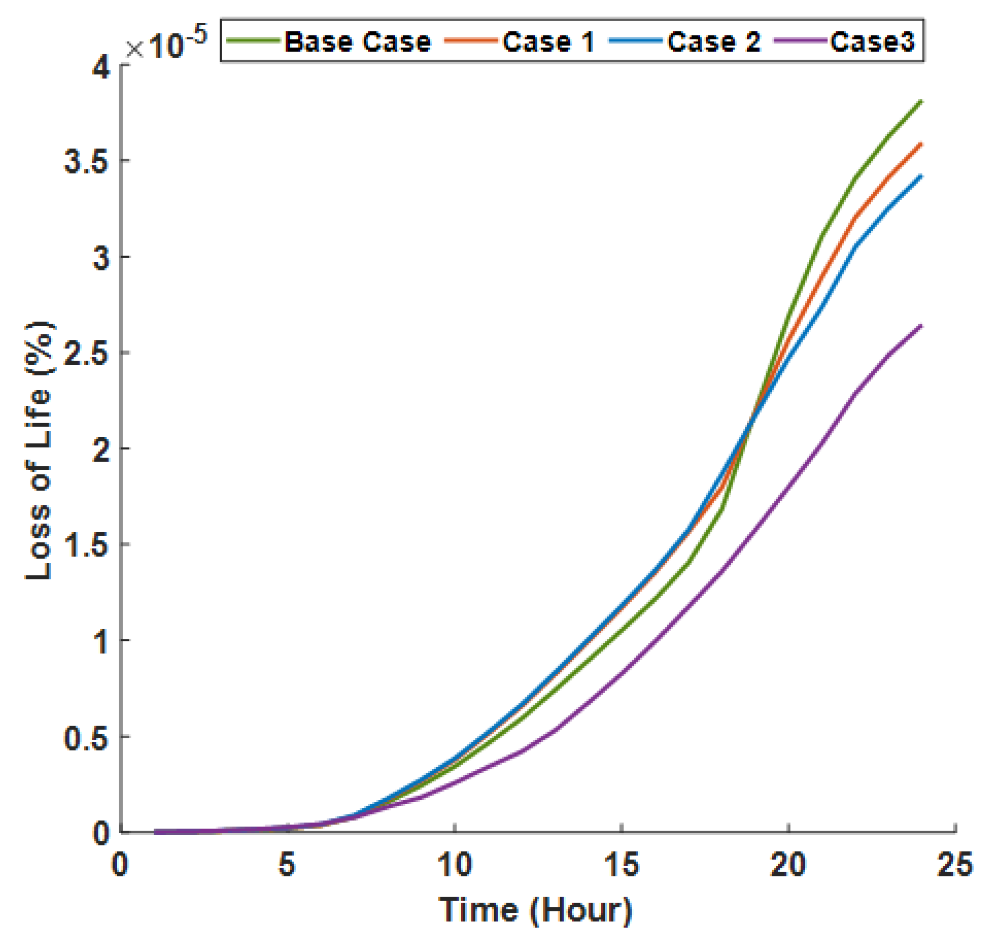
  • Introducing the LoL cost of a distribution transformer into the optimization model. A transformer thermal model is used to calculate the LoL cost, and the DR multi-objective model is developed to support the asset condition while maximizing the utilization capacity of the distribution transformer.
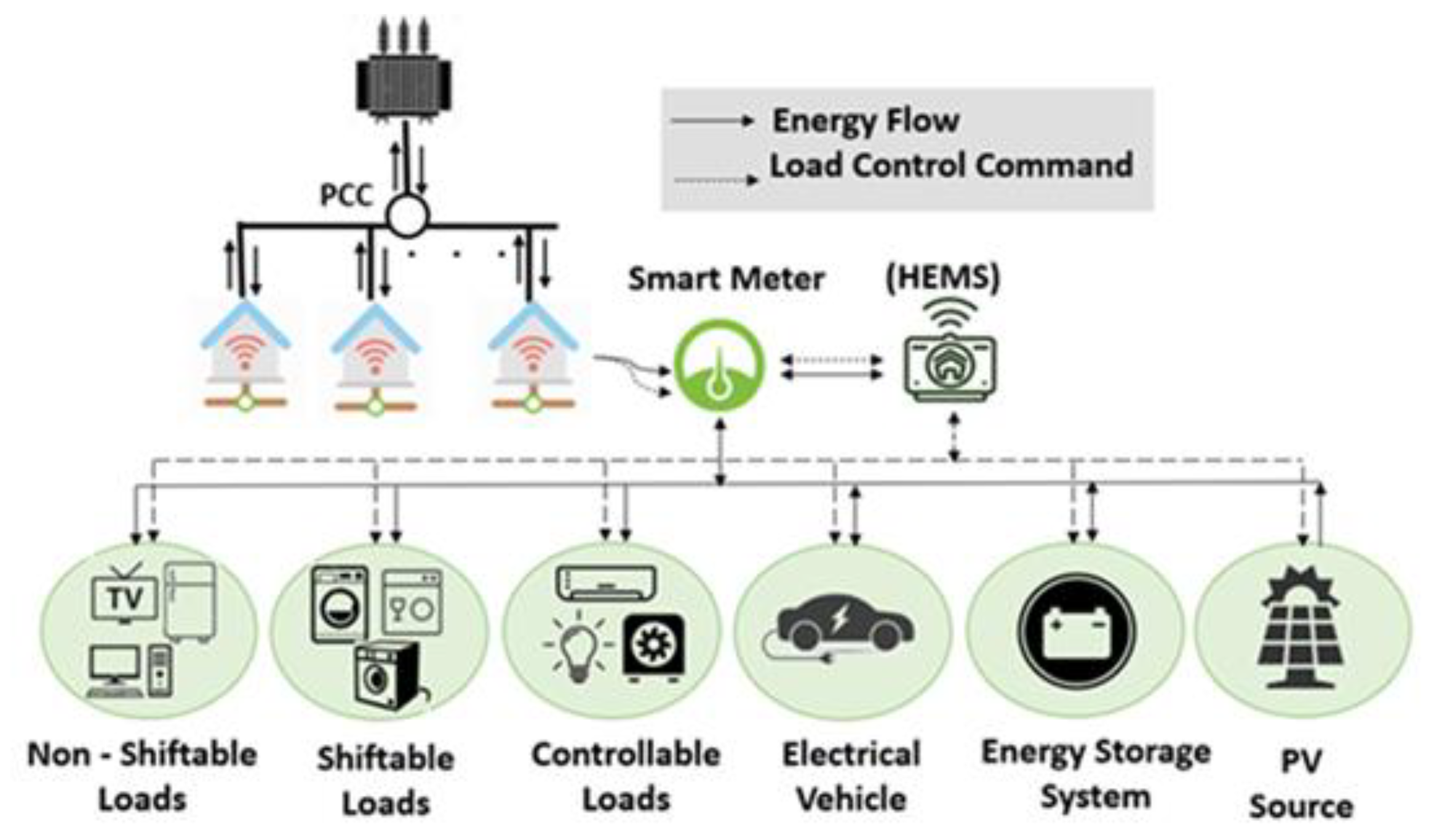
  • Integrating PV, ESS, EV, and all types of non-shiftable, shiftable, and controllable appliances in a DR program considering end-user preferences.
The rest of the paper is organized as follows. The DR optimization problem formulation is presented in Section 2. Section 3 presents the application of the proposed model and simulation results. An evaluation of the algorithm and a discussion on its application results are introduced in Section 4. Concluding remarks are presented in Section 5.

2. Optimization Problem Formulation

The proposed DR framework can be mathematically expressed as an optimization problem with various objectives and constraints, as shown in Figure 2. The optimization problem is formulated based on PV generation, asset degradation costs, electricity price, initial state of energy (SoE) of EVs, and ESSs’ batteries, together with the user preferences data. Each of these elements is described in detail in the below subsections.

2.1. Weighted Objective Function

The multi-objective function is presented as a cost model that consists of electricity charge cost considering transformer LoL ( F 1 ) and customer dissatisfaction cost ( F 2 ), which are weighted and combined into a single objective function, as shown in Equation (1).
min   ρ   F 1 + ( 1 ρ )   F 2       ρ   [ 0 ,   1 ]
This integration allows the customers and operators to decide the combinations that better fit their economic interests and meet their technical requirements. This can be done by adjusting the customer/operator balance parameter ρ to achieve the trade-off between F 1 and F 2 . These sub-objective functions are presented as:
F 1 = n = 1 N h = 1 H   C n , h + C h T x
F 2 = n = 1 N h = 1 H   c d c n , h
The model in F 1 presents the electricity charge cost and the transformer LoL cost, which is directly related to the asset condition. If the value of C n , h   is positive, the consumed power is from the grid. Otherwise, if the value of C n , h   is negative, the consumed power is from after-the-meter-generated power based on DERs and BESSs. F 2 is introduced to capture the degree of discomfort caused to the customer due to the DR schedules.

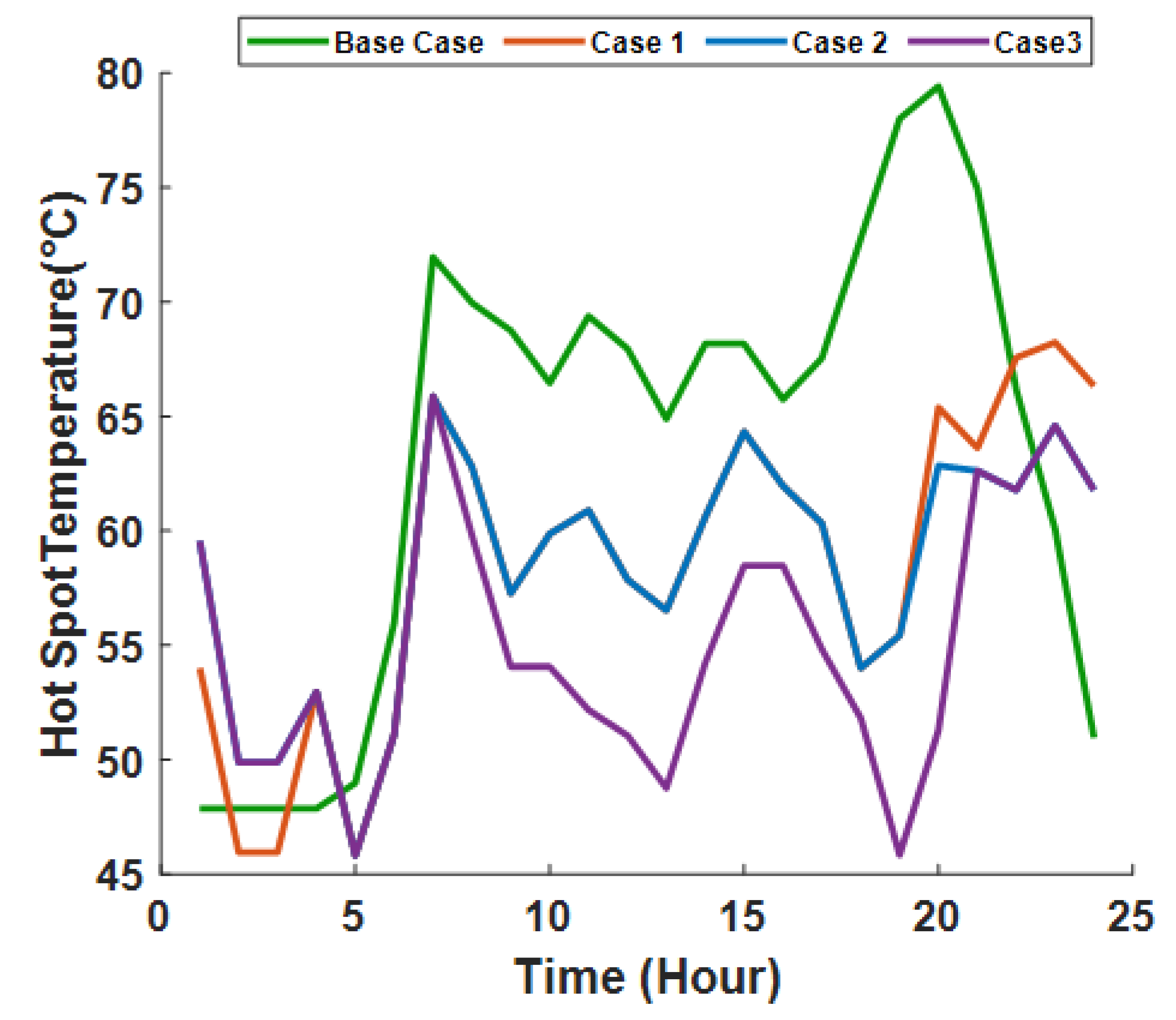
2.2. Transformer LoL Mitigation

The main cause of failure of distribution transformers is prolonged overloading. Thermal management of a transformer can improve its operation by managing the transformer LoL. The main two parameters used to approximate a transformer’s lifetime are transformer winding top oil temperature (TOT) and transformer winding hot spot temperature (HST). A precise thermal model of the distribution transformer can minimize the LoL and maximize the transformer utilization [24]. External and internal factors can affect the transformer’s thermal behavior such as ambient temperature and the transformer’s loading. Increasing ambient temperature results in an increase in the operating temperature of transformers. Ref. [25] states that for every 10 ℃ increase in ambient temperature, the lifetime of distribution transformers will be reduced two times faster than the normal operation. According to [26], when the HST reaches 140 ℃, the relative aging rate reaches 100. This means that operating the transformer for one hour at overloading conditions equals 100 operating hours at normal operation. Any increase in the ambient temperature or transformer loading levels leads to an increase in the transformer HST. Thus, the transformer loading conditions depend on the HST and ambient temperature [27].
Based on the price signal received from the utility, the DR program intends to allocate the load during the lowest-price time. However, high penetration of scheduled household loads during these periods raises a concern of new high-power peaks that leads to distribution transformer overloading with high LoL. Hence the objective function F 1 is introduced to reflect the transformer LoL degradation cost in the DR optimization program. This degradation cost at a particular time depends on the transformer load, ambient temperature, and the %LoL at that time. The IEEE standard C57.91-2011 is used to determine %LoL of the distribution transformer, and it consists of three variables: ambient temperature, winding hottest-spot temperature, and top oil temperature [27]. It is given by Equation (4).
θ H = θ A + Δ θ H + θ T O
where Δ θ H calculates the increase in the oil and winding temperature caused by the increase in transformer current as given by Equation (5). The initial value of top oil temperature rise over ambient is given by Equation (6), and the ultimate top oil temperature rise is given by Equation (7)
Δ θ H = (   Δ θ H , u Δ θ H , i ) ( 1 e x p t τ H ) + Δ θ H , i
Δ θ H , u =   Δ θ H , R [ k u ] 2 m
Δ θ H , i =   Δ θ H , R [ k i ] 2 m
Equation (8) presents the top oil rise over ambient temperature. As seen from Equation (9), any increase in the transformer current will increase the overall transformer temperature. The ultimate and initial top oil rise temperatures are given by Equations (9) and (10), respectively.
Δ θ T O = (   Δ θ T O , u Δ θ T O , i ) ( 1 e x p t τ T O ) + Δ θ T O , i
Δ θ T O , u =   Δ θ T O , R [ k u 2 · R + 1 R + 1 ] n
Δ θ T O , i =   Δ θ T O , R [ k i 2 · R +   1 R + 1 ] n
This model is based on the effect of the HST on the aging of the distribution transformer. The relation of the aging acceleration factor and the transformer’s hot spot temperature (reference temperature 110 °C) is expressed in Equation (11).
F A A = exp ( 1500 383 1500 θ H + 273 )
The equivalent aging factor at the reference temperature at a given time can be used for calculating the loss of life, as shown in Equation (12).
F E Q A = r = 1 N F A A , r Δ t r Δ t r
Equation (13) is used to determine the percent LoL. The normal insulation loss of life is considered to be 180,000 h (20.55 years).
% L O L = F E Q A × t × 100 N o r a l   I n s u l a t i o n   l i f e
The transformer capacity total cost is utilized instead of a fixed threshold constraint, and the LoL cost is estimated using Equation (14) [28].
C h T x   = T r a n s f o r m e r   i n v e s m e n t   c o s t N o r m a l   l i f e   e x p e c t a n c y   × L O L h %

2.3. Home Appliance Constraints

The use of different categories of home appliances needs to be managed so that the total cost of electricity can be minimized considering electricity price as a function of the time interval and customer comfort. The appliances’ operation and user preferences limit scheduling. Therefore, household appliances are categorized and modeled according to their configuration and their effect on user comfort. Some attributes considered for the appliances, for example, are as follows:
  • ID number (n).
  • Scheduling window ( [ T n , i n t , T n , e n d ] ).
  • Importance parameter ( ζ n ).
  • Power rating ( E n , h   ).
  • Operating time duration ( T n , e n d ).
The mathematical model for each category of appliances, along with its constraints, is explained in the following subsections.

2.3.1. Non-Shiftable Appliances

Non-shiftable loads have a critical operating status which is always “on” and cannot be scheduled or controlled, such as refrigerators and alarm systems. The cost of such loads is presented by Equation (15).
C n , h   = λ h · E n , h  

2.3.2. Shiftable Appliances

Shiftable loads, i.e., washing machine and clothes dryer, can be scheduled for off-peak hours when the electricity cost is low. The consumption cost for these appliances is represented by (16). Furthermore, the limits for the shiftable appliance n throughout the scheduling horizon should satisfy the constraints in Equations (17) and (18).
C n , h   = λ h · u n , h   · E n , h  
u n , h   = 0         h [ 1 , T n , i n t )     ( T n , e n d , H ]
u n , h   1         h [ T n , i n t , T n , e n d ]
Equation (19) reflects the customer’s dissatisfaction with waiting for the appliance to start the operation. Minimizing Equation (20) leads to minimizing the waiting time as much as possible, which supports customer comfort.
c d c n , h =   ζ n ( T n , s t a r t   T n , i n t )
T n , i n t   T n , s t a r t   ( T n , e n d T n , t o t a l )

2.3.3. Controlled Appliances (Active Loads)

This category of appliances has flexible power consumption, such as lights and air conditioners. Their power consumption can be regulated between the maximum and minimum in response to price changes. Controlling these loads supports minimizing the customer electricity bill, as presented in Equations (21) and (22). Nonetheless, power reduction can cause dissatisfaction for the customer, as presented by Equation (23).
e n , m i n E n , h     e n , m a x
C n , h   = λ h · E n , h  
c d c n , h = ζ n ( E n , h   e n , m a x ) 2

2.4. Electrical Vehicle Constraints

The EV model supports the engagement of customers in the energy market. Charging and discharging of the EV battery is controlled based on the electricity price and the asset condition. The EV charging/discharging cost is presented by Equation (24). Equation (25) presents the difference between the EV’s maximum energy and the actual charged energy, multiplied by a dissatisfaction factor that penalizes not having a fully charged EV at departure time. Constraints in Equation (26) define the discharge power usage from EV (V2H or V2G). The amount of energy available in an EV battery at time h is presented by Equations (27) and (28). The EV battery stored energy is limited between minimum and maximum values to prevent deep discharging or full charging, as presented by Equation (29).
C n , h   = { λ h · E n , h E V / c     λ h · E n , h E V / d
c d c n , h = ζ n ( S O E n , h E V S O E n E V / m a x ) 2   i f   h = h n d e p
E n , h E V / u s e d + E n , h E V / s o l d =   η E V / d · E n , h E V / d   h [ h n a r r , h n d e p ]
S O E n , h E V =   S O E n E V / i n t + η E V / c · E n , h E V / c E n , h E V / d   , i f   h = h n a r r
S O E n , h E V =   S O E t 1 E V + η E V / c · E n , h E V / c E n , h E V / d   h ( h n a r r , h n d e p ]
S O E n E V / m i n S O E n , h E V S O E n E V / m a x

2.5. Energy Storage System Constraints

The ESS is modeled in a similar way to EV, as presented by Equations (31)–(35). However, according to the DR program, the ESS is available all day at the house to be utilized (charging/discharging).
C n , h   = { λ h · E n , h E S S / c λ h · E n , h E S S / d
c d c n , h = { ζ n ( S O E n , h E S S S O E n E S S / m a x )   2   i f     S O E n , h > S O E E S S / m a x   , ζ n ( S O E n , h E S S S O E n E S S / m i n ) 2     i f     S O E n h < S O E E S S / m i n , 0                                   o t h e w i s e ,
E n , h E S S / u s e d + E n , h E S S / s o l d =   η E S S / d E n , h E V / d
S O E n , h E S S =   S O E t 1 E S S + η E S S / c · E n , h E S S / c E n , h E S / d   h > 1
S O E n , h E S S =   S O E n E S S / i n t , i f   h = 1
S O E n E S S / m i n S O E n , h E S S   S O E n E S S / m a x

2.6. PV Model Constraints

PV energy resources further support customer engagement in the energy market. Equation (36) implies that the generated power from PVs can be used by the household appliances or injected back to the grid based on the DR contract between the utility and the prosumer.
P h P V =   P h P V / u s e d + P h P V / s o l d

2.7. Power-Limiting Strategies

Flattening the load profile is one of the main criteria which should be considered in DR strategies. Beside the transformer thermal model, utilities can provide several incentive power-limiting strategies to the households according to the DR program they participate in [8]. This would reduce the peaks of demand, which generates benefits for the whole system. The reward for consumers is direct since they pay less by following a particular strategy. For instance, during coincident peak periods, the utility can impose a limit on the power drawn by the users to reduce the power system peak. A power-limiting strategy may also control the customer’s daily power consumption pattern, as presented in Equations (37) and (38). However, If the user needs to use a power that exceeds the defined limit, the excessive energy usage will be charged by a higher price, e.g., a coincident peak charge, so a significant cost reduction can be realized if the user reduces the demand at peak hours.
m a x h ( P h g P h s o l d ) Γ
P h g l h · u h

2.8. Implementation Considerations

To execute the formulated DR optimization problem, several considerations and assumptions are made. These assumptions and considerations come under two main categories: (i) predictions of the model input data and (ii) executing the scheduled load proposed by the HEMS. Each of these points is examined by prior literature, as highlighted in the following paragraphs.
The user has a DR contract with the utility. This DR contract is categorized by different periods: off-peak, demand peak, and coincident peak. The off-peak price can be fixed throughout the day or time-varying, depending on the electricity market. Usually, λ h   is in the order of several cents per kWh. This paper assumes a real-time pricing (RTP) scheme at off-peak times. The peak demand charge, also known as a power tariff, is applied during the hours where the customer consumption is high. Customers are motivated to decrease their consumption by increasing the power tariff as their peak demand increases. This charge is obtained by determining the hour of the day/month when the user’s consumption is maximal. Here, λ h   is much higher than in the off-peak charge. It can reach several dollars per kWh. The coincident peak pricing scheme is the same as the peak charge scheme but manages the peak hour for the utility instead of the peak for each consumer. This is done by determining the utility’s peak hour at the end of each day/month. After that, all users pay for their electricity consumption at this time. The rate of these charges can reach a price that is more than the peak demand charge rate [29].
The paper assumes that the hourly energy cost ( λ h ) is known for each end-user. This price is not the accurate price that the user will pay, but it indicates the next day’s expected prices. The utility announces the actual price in real-time, a common procedure in real life [30]. Besides, to aid customers, the utility should have the Peak Alert DR program in which they issue alerts notifying participants of potential peak hours each day/month. This program simply provides forecasted alerts. In practice, price and coincident peak predictions can be made using historical data that are generally available by the utilities’ operating demand response programs. Other parameters needed by the algorithm are considered perfectly known and can be fairly predictable in practice. For example, the algorithm needs the predicted renewable generation and transformer load as inputs. The input data prediction can be made in many ways, e.g., [31,32]. In practice, the household owner may set the appliances’ information according to their needs, or an intelligent system that learns the household owner’s behavior could be adapted.
Given the predictions for the coincident peak, transformer load, electricity price, renewable generation, etc., the proposed algorithms make ideal energy scheduling decisions to fulfill the optimization problem objectives since the optimization problem is convex. In a simple form, it can be solved efficiently. For simplicity, the ESS degradation cost is neglected. Given the resulting energy schedule, the remaining work is implementing and consolidating the HEMS at the household level.

3. Application and Results

3.1. Simulation Data

The mathematical model described in the previous section was implemented in MATLAB using the Interior Point Method, which solves linear and non-linear convex optimization problems. The simulations were conducted on one household and three houses supplied from a distribution transformer to demonstrate the benefits of the proposed methodology on the prosumer and the utility operator. It was assumed that all the input data are known for the algorithm. Table 1 presents different kinds of active and passive appliances with different configurations using the appliance importance coefficients. The CDC weights in Table 2 are defined by the prosumer considering the energy price variation within the day, and the balance parameter ( ρ ) is set to 0.5. The after-the-meter DER data within each household are estimated as in Table 2 [33]. The PV source was designed to meet about 10% of the total load for 24 h. Table 1 and Table 2 parameters are varied for each household according to the characteristics of the appliances and the end-user preference as well as the available DERs.

3.2. Results and Discussion

This section demonstrates the simulation and performance evaluation results carried out by MATLAB to analyze the optimal load management in smart home integrated considering different cases. The proposed DR algorithm is applied to compare the following three operating cases with a base case representing a reference without using the proposed algorithm. The capability of the HEMS to sell the extra energy back to the grid complicates the simulation analysis. Besides, there are many policies regarding the injected energy to the grid, requiring separate analysis. In this respect, selling energy back to the grid is out of the scope of this paper.

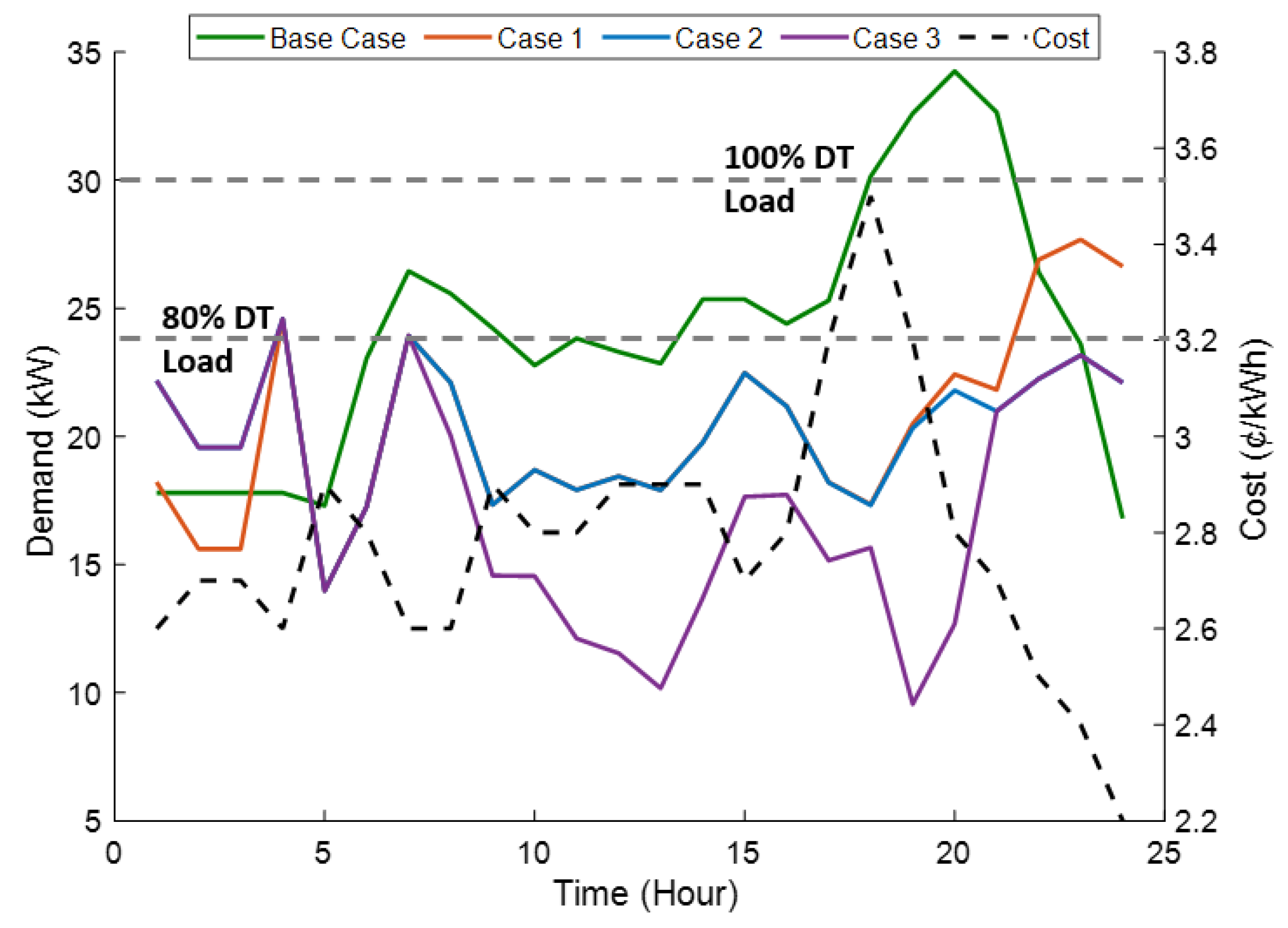
3.2.1. Base Case: Without the DR Program

This case is considered as a reference in the study, which presents the household load profile before participating in the DR program. Figure 3 shows the aggregated energy consumption of all active and passive household loads, as well as the signal of energy cost. Based on the cost signal, the estimated energy consumption cost of the reference case is USD 6.1.

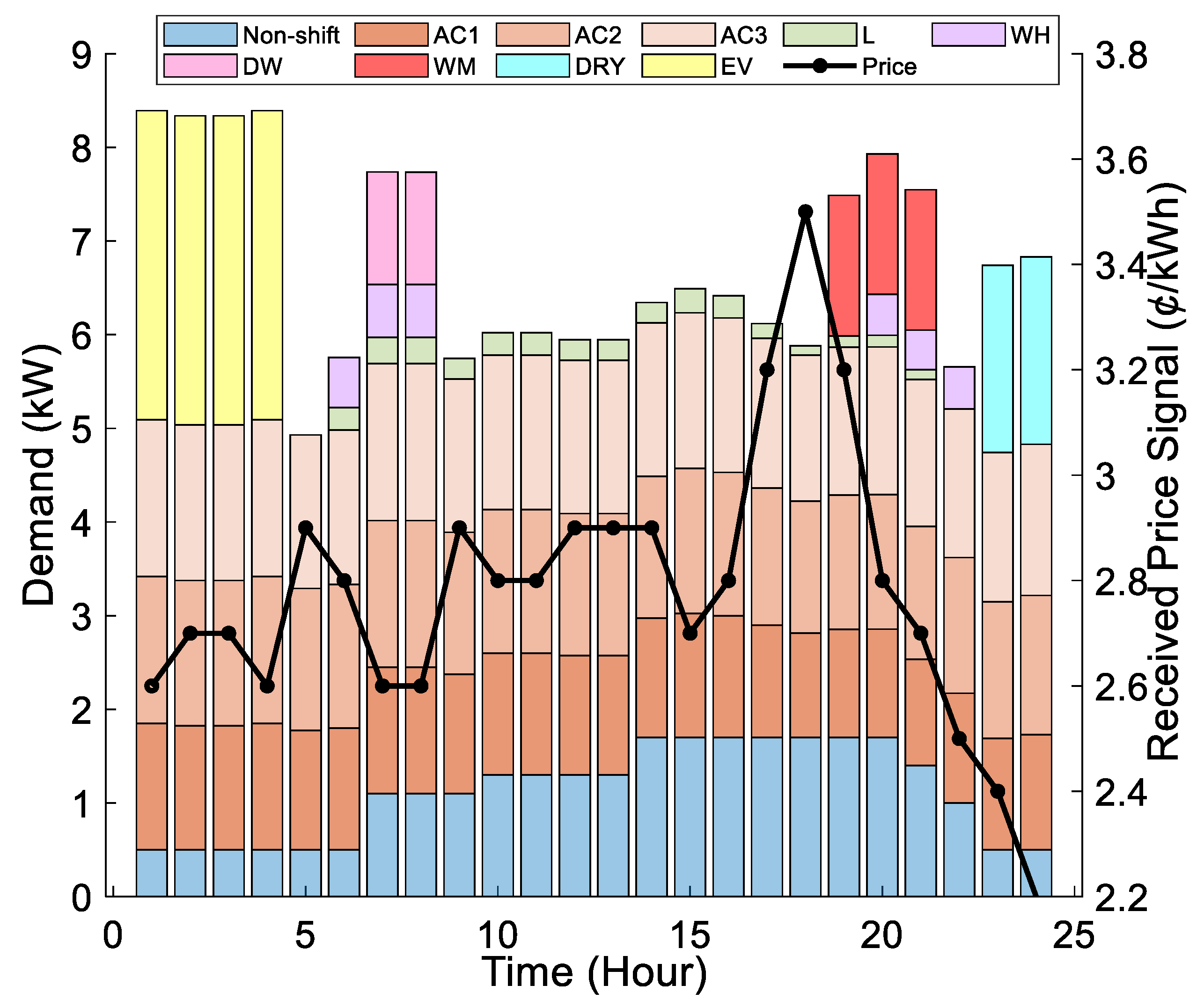
3.2.2. Case 1: The Impact of Customer Dissatisfaction Cost

The objective, in this case, is to minimize the total daily operation cost considering the CDC ( F 2 ) and ignoring the transformer LoL cost in Equation (2). The customer comfort level is reflected in the optimization algorithm, considering the ζ n parameter, as illustrated in Table 1. Figure 4 shows the aggregated household load along with the electricity price signal after participating in Case 1. The proposed DR algorithm attempts to optimize energy consumption and achieve the lowest electricity charge cost. Specifically, all active loads (controllable and shiftable loads) are scheduled to operate outside electricity high-price slots. The controllable loads are scheduled to consume less energy from 15:00 to 20:00 and consume more energy between 1:00 and 8:00 and 21:00 and 24:00. The shiftable loads (DRY and WM) are scheduled to operate at 23:00 and 24:00, where the electricity price is low. The DW remains operating in slots 7 and 8 as it is the lowest in its working period, as specified in Table 1. The DR algorithm reduced the operation cost by scheduling the EV charging in the lowest price slots (22:00–24:00 and 4:00) during the time that EV is at home.
Also, it can be observed that appliances with larger ζ n consume more energy than the appliances with lower ζ n . This is to guarantee that the customer suffers less dissatisfaction with the proposed DR algorithm. For example, for the same electricity price, AC3 consumes more energy than AC2, and AC2 consumes more energy than AC1.
The electricity consumption cost of implementing Case 1 is USD 4.5, 25% less than the reference case. End-users’ engagement in the DR program depends on the class of customers. Technology supporters have the potential to participate in such a HEMS-DR program and other energy market opportunities. However, another class of end-users still presents a challenge and may need additional incentives for engagement, even with the electricity cost reduction achievement. Hence, full engagement in this program is limited to the technology-supporter class of customers. Furthermore, having individual control of the DR algorithm per individual end-user may cause the low-cost periods to operate as a sink for all customers to operate their appliances during these intervals and generate new load peaks detected by utility assets.

3.2.3. Case 2: The Impact of Transformer LoL Cost

In this case, the objective function of transformer LoL mitigation cost is considered along with operation cost ( F 1 ), as presented in Equation (2), and customer discomfort cost ( F 2 ). The HEMS implements an approach to fulfill the consumer’s expectations and decreases the transformer’s LoL by monitoring transformer load, electricity price, HST of distribution transformer, and predicted consumption pattern of the customer. The DR program’s impact on a 30-kVA distribution transformer based on the IEEE standard C57.91-2011 is used to investigate its loss-of-life cost. The transformer is assumed to be supplying three houses where their household loads are monitored and controlled by the proposed DR algorithm. Based on Case 1, the transformer has a peak demand in lower-price slots as the DR algorithm operates all the smart appliances in these periods. Therefore, the load and LoL factor during these periods increased compared with the reference case’s low-price periods.
The DR algorithm overcomes this issue by including the LoL as a transformer deterioration cost using (5). Figure 5 shows the Case 2 optimized scheduling for the household load after adding LoL cost. It can be noted that the EV charging load is shifted to slots 1:00–3:00 of high electricity price compared to slots 22:00–24:00 used in Case 1. While this load shift may increase the electricity cost, it satisfies the LoL cost and overcomes the distribution transformer’s overload condition and other assets. Case 2 results in a peak demand reduction of 18% compared to Case 1, positively impacting the utility assets. The new load profile of Case 2 has an electricity cost of USD 4.7, which is higher than Case 1; however, it is lower than the base case by 23% and provides direct benefits to both the end-user and utility operator.

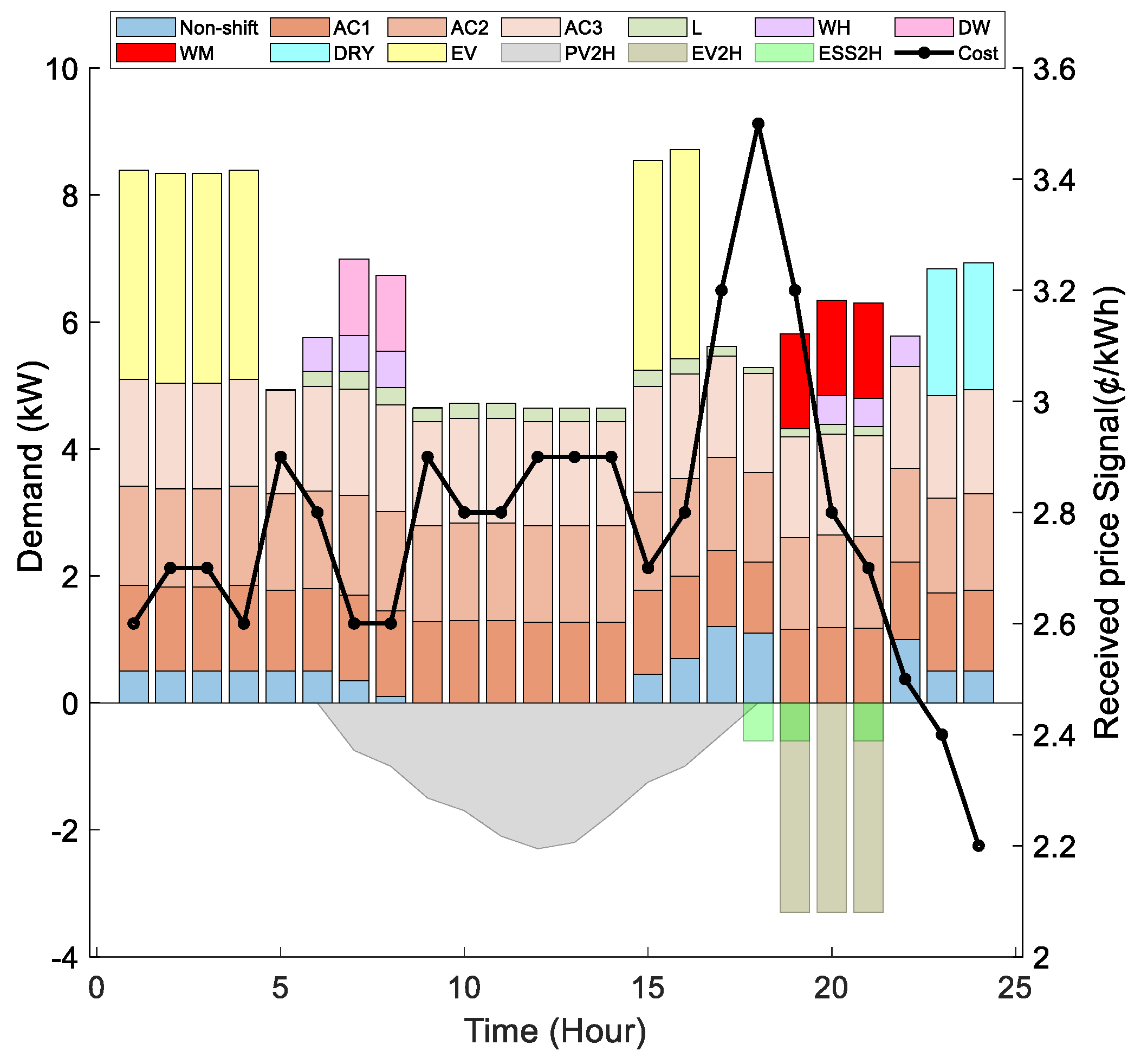
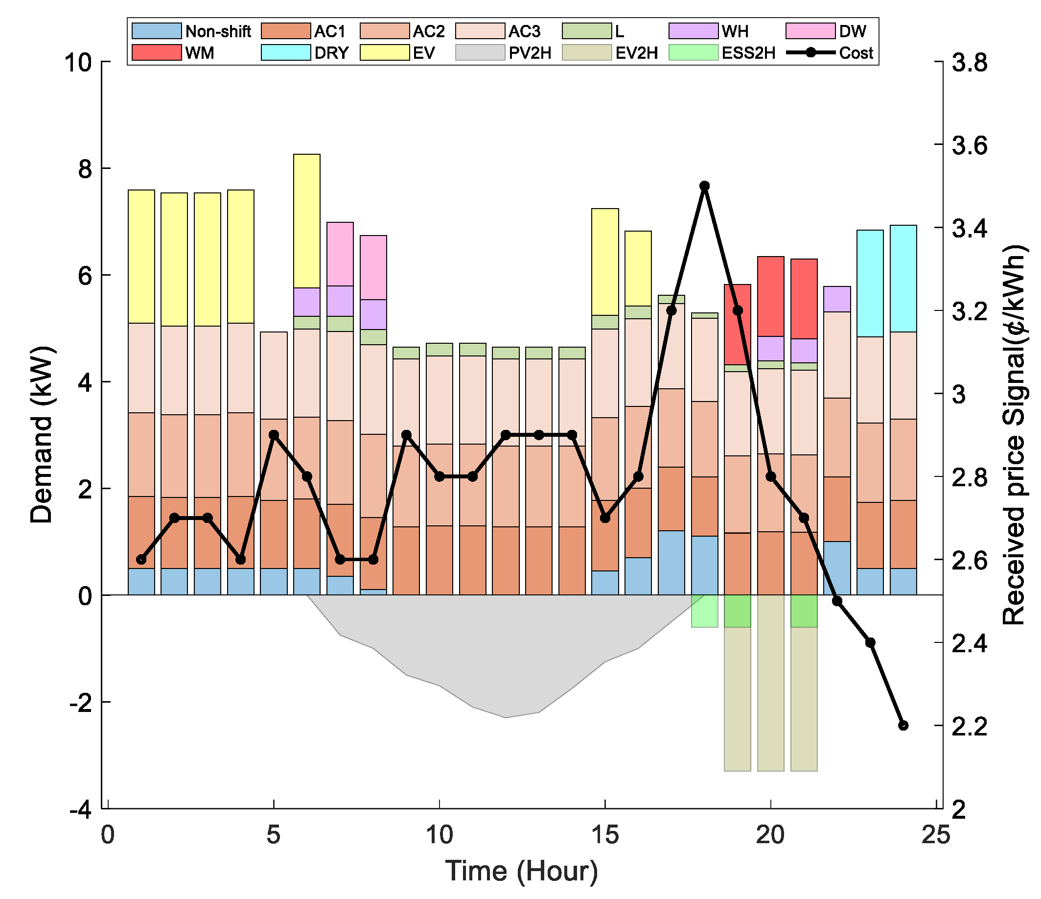
3.2.4. Case 3: The Impact of DERs

DERs are essential in developing active customers with the potential to engage in the local energy market and, hence, are integrated into the HEMS-DR program. This case emphasizes the DR algorithm’s benefits by utilizing assets such as PVs, ESSs, and EVs. The energy offered by the household assets (PV, EV, and ESS) is used to minimize consumption from the grid and balance the demand/generation relationship. It is assumed that PV-to-home (PV2H), ESS-to-home (ESS2H), and EV-to-home (V2H) capabilities are available. These assets may also be used to sell energy to the grid via PV-to-grid (PV2G), V2G, and ESS2G options. Figure 6 presents the results of this case, and the following are observed:
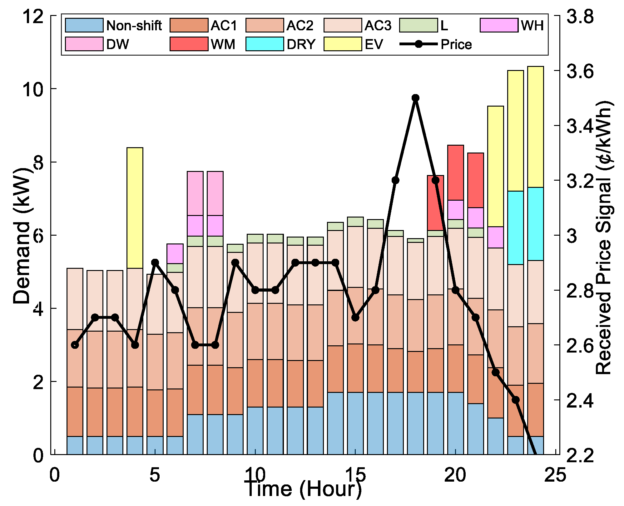
  • The PV-generated power is used to partially cover the demand and charge the ESS as long as it is available.
  • When prices are high, the ESS’ available energy is utilized to cover part of the load and reduce electricity consumption cost, as illustrated during the 17:00–19:00 time period.
  • As the EV arrives at the household, it contributes to the energy needs from 19:00 to 2:00 with sufficient energy. It is also observed that the HEMS-DR algorithm avoids chagrining the EV in high price slots.
The electricity cost of case 3 is USD 4.2, which is 31% lower than the base case, 9% lower than Case 1, and 10% lower than Case 2.

4. Performance Evaluation

4.1. The Impact of Power Limiting Strategy

The presented algorithm aims to operate the household loads when the price is low and respond to the utility’s specific load-shape requirements. To evaluate this, a power limit restriction is enforced throughout the time horizon to limit the drawn energy from the grid to a maximum value of 8 kWh to reduce the customer peak demand, as presented in Equation (38). Violating the power limit is allowed under a penalty that is equal to the demand charge tariff. The demand charged is assumed to be equal to 110% of the day’s highest electricity price (3.8 cents). As shown in Figure 7, under this strategy, the total peak is further decreased to 8 kW, and as a result, the EV charging is reduced and the charging period is increased. However, the load stays the same as the previously discussed case (Case 3).

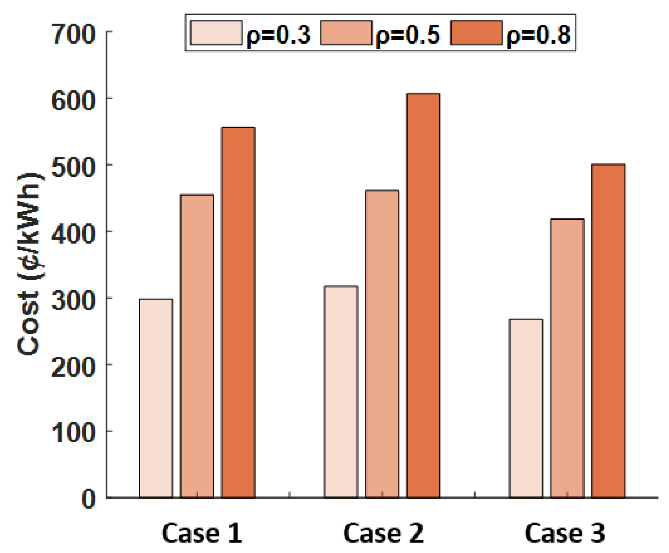
4.2. The Impact of the Balance Parameter ρ

The balance parameter for customer and utility benefits directly impacts the objective function in Equation (1). Figure 8 shows the electricity consumption cost of the three previously mentioned cases using the proposed DR program under different customer-utility balance parameters (ρ). A large value of ρ magnifies the energy operation cost and the transformer LoL mitigation cost ( F 1 ) in the objective function. On the other hand, using a small ρ magnifies the customer dissatisfaction cost ( F 2 ) in the objective function, where the end-user has more impact on the cost function compared with the utility. Hence, selecting the value of ρ is an essential element in the optimization algorithm and should be defined based on a mutual agreement that reflects the customer and utility operator benefits.

4.3. The Impact of DR Program on Distribution Transformer

The impact of the DR program’s three cases on a distribution transformer (DT) loading condition is studied. The active loads of three houses are used, and the DERs are randomly varied within the ranges specified in Table 1 and Table 2. The aggregated load of the five houses supplied by a 30-kVA distribution transformer is estimated, and the results of the DR program of the previous cases are illustrated in Figure 9. The price pattern is also included in the figure to help in result analysis. To evaluate the proposed DR algorithm’s efficacy, the base case is considered with a severe loading where the DT loading condition shows 4-h continuous overloading above 100% rating during the 18:00–22:00 time interval and another 10 h above 80% rating. Case 1 of the DR program supports customers’ benefit in energy cost reduction. However, the results present an alarming indication of a possible overloading condition that accelerates transformer degradation. Furthermore, part of the overloading conditions time intervals has a low-price signal, which may work as a sink for other customers to operate their appliances, and that magnifies the load peak condition of the DT. Implementing Case 2 of the DR program shows a reduction in the DT load beyond the 80% rating and an increase in the energy cost due to load shifting to high-price electricity cost intervals. This is shown in the figure during the time intervals 1:00–4:00 and 20:00–24:00. Case 1 and Case 2 of the DR program show similar responses during the time interval 4:00–20:00. Including DERs in the DR program (Case 3) shows the optimal operation scenario as expected. The DR program generates a DT loading below all the cases during the time interval from 7:00 to 19:00 and merges with the lowest case (Case 2) during the time intervals 4:00–7:00 and 19:00–24:00.
According to Equations (5)–(14), the HST of the transformer will be raised during overloads. As shown in Figure 10, the HST reached around 73 °C without DR, and with the DR, the average and maximum HST for transformers have been reduced in all the cases. Since the HST has a significant impact on the aging of transformers, minimizing HST will minimize transformer LoL%. As shown in Figure 11, the LoL of a transformer can be reduced by up to 25% by the proposed DR algorithm. A comparison of the total transformer load, HST, and LoL% is shown in Table 3.

4.4. Challenges and Opportunities

One of the chief benefits of the proposed model is its flexibility. It can be automatically adjusted and adapted to consider more appliances and constraints and generate the best possible scheduling solutions. The equations can be solved in more than one way. The result in this paper was obtained using a laptop (i7 at 2.6 GHz, 16 GB of RAM, 64-bit Windows) with a computation time, on average, of 5 s. With a more powerful processor and high-capacity RAM, the computation time will be further reduced. However, implementing such an algorithm for larger-scale applications may increase the computational burden. Since the computational complexity of the scheduling problem is non-polynomial (NP)-hard, as the number of constraints and variables increases, the developed model’s computational time exponentially increases. In this case, heuristics approaches are useful for reducing the computational burden of the scheduling problem and capable of approximating the optimal solutions in a reasonable time. However, a detailed analysis of the computational complexity would be necessary in order to fully evaluate its potential for future large-scale applications.

5. Conclusions

The paper proposes a multi-objective residential DR optimization model that coordinates the benefits of households and utility operators. The model aims to minimize the individual household electricity consumption cost while considering customers’ comfort and lifestyle. The utility distribution transformer’s load profile is integrated into the optimization model by incorporating the asset loss-of-life (LoL) cost in the multi-objective function. The proposed model’s flexibility is supported by considering various demand/generation components that consume/produce electricity. The proposed algorithm’s application is presented by three operation scenarios, compared with a reference case, and illustrated customers’ and operators’ benefits in terms of consumption cost, customer discomfort cost, and transformer asset load leveling. The results of the multi-objective DR model revealed a 38% reduction in the electricity consumption cost and an 18% reduction in the aggregated peak demand of the distribution transformer.
In future work, peer-to-peer energy trading and two-way energy trading with the grid will be considered as an extension of the current work, increasing the HEMS’ economic benefits. The appliance’s uncertainty will also be considered by detecting the heterogeneity in demand at the device level by the DR algorithm.

Author Contributions

Conceptualization, A.A., K.S. and A.M.; methodology, A.A.; software, A.A.; validation, K.S., A.G. and A.M.; formal analysis, A.A.; investigation, A.A.; resources, K.S.; writing—original draft preparation, A.A.; writing—review and editing, K.S., A.G. and A.M.; All authors have read and agreed to the published version of the manuscript.

Funding

This research was funded by the NPRP11S-1202-170052 grant from Qatar National Research Fund (a member of the Qatar Foundation). The statements made herein are solely the responsibility of the authors.

Institutional Review Board Statement

Not applicable.

Informed Consent Statement

Not applicable.

Data Availability Statement

Data is contained within the article.

Conflicts of Interest

The authors declare no conflict of interest.

Nomenclature

h ( H ) Index (set) of time periods.
n ( N ) Index (set) of household appliances.
ρ Balance parameter for customer/utility benefits.
F 1 Transformer LoL mitigation objective function.
F 2 Electricity cost objective function.
F 3 Customer dissatisfaction cost objective function.
λ h   Hourly electricity cost (¢/kWh).
P n , h s o l d Total power sold back to the grid (kW).
C h T x The transformer LoL cost at time h .
c d c n , h Dissatisfaction cost for appliance n at time h .
C n , h Electricity cost for appliance n at time h .
E n , h Consumption for appliance n at period h (kWh).
e n , m a x Maximum consumption for appliance n (kWh).
e n , m i n Minimum consumption for appliance n (kWh).
u n , h   Appliance status in household ∈ {0,1}.
ζ n Appliances dissatisfaction coefficient.
T n , s t a r t Operation starting time.
T n , i n t Initial time of working period.
T n , e n d End time of the working period.
T n , t o t a l Appliance required operation time.
E n , h E V Energy accumulated in EV battery (kWh).
E n , h E V / m a x Maximum energy in EV battery (kWh).
E n , h E V / m i n Minimum energy in EV battery (kWh).
E n , h E V / u s e d Power used by appliances fed by EV (kW).
E n , h E V / s o l d Power injected to grid from EV (kW).
η E V / c EV battery charging efficiency factor.
η E V / d EV battery discharging efficiency factor.
S O E E V / i n t Initial state of the EV battery (kWh).
S O E n , h E V / m i n Minimum SoE of EV (kWh).
S O E n , h E V / m a x Maximum SoE of EV (kWh).
S O E n , h E V EV SOE (kWh).
E n , h E S S / s o l d Power injected to grid from ESS (kW).
E n , h E S S / u s e d Power used by appliances from ESS (kW).
η E S S / c ESS charging efficiency factor.
η E S S / d ESS discharging efficiency factor.
S O E E S S / i n t Initial state of the ESS (kWh).
S O E n , h E S S / m i n Minimum SOE of ESS (kWh).
S O E n , h E S S / m a x Maximum SOE of ESS (kWh).
S O E n , h E S S ESS SOE (kWh).
h n a r r , h n d e p EV arrival/departure time.
P h G Flow of energy between household and grid.
l h Time-varying power limit for the power drawn from the grid (kW).
u h g Binary variable—1 if power is drawn from the grid, else 0.
θ H Transformer winding HST.
θ A Ambient temperature in °C
Δ θ H Winding hottest-spot rise over the top-oil temperature in °C
θ T O Hot spot rise over top oil temperature in °C
Δ θ H , u Ultimate hottest-spot rise over top-oil temperature.
Δ θ H , i Initial hottest-spot rise over top-oil temperature
τ H Winding hot spot time constant in hours.
Δ θ H , R Rated hot spot rise over top oil temperature.
k u Ratio of ultimate to rated load in per unit.
k i Ratio of initial to rated load in per unit
R Load loss ratio.
Δ θ T O , u Ultimate top oil rise temperature,
Δ θ T O , i Initial top oil rise temperature.
τ T O Oil hot spot time constant in hours.
Δ θ T O , R Rated top oil over ambient temperature.
F A A Aging acceleration factor
F A A , r Aging acceleration factor for time interval Δ t r .

References

  1. Vardakas, J.S.; Zorba, N.; Verikoukis, C.V. A Survey on Demand Response Programs in Smart Grids: Pricing Methods and Optimization Algorithms. IEEE Commun. Surv. Tutor. 2015, 17, 152–178, First quarter. [Google Scholar] [CrossRef]
  2. Shareef, H.; Ahmed, M.S.; Mohamed, A.; Al Hassan, E. Review on Home Energy Management System Considering Demand Responses, Smart Technologies, and Intelligent Controllers. IEEE Access 2018, 6, 24498–24509. [Google Scholar] [CrossRef]
  3. Khalid, A.; Javaid, N.; Guizani, M.; Alhussein, M.; Aurangzeb, K.; Ilahi, M. Towards Dynamic Coordination Among Home Appliances Using Multi-Objective Energy Optimization for Demand Side Management in Smart Buildings. IEEE Access 2018, 6, 19509–19529. [Google Scholar] [CrossRef]
  4. Amini, M.H.; Frye, J.; Ilic´, M.D.; Karabasoglu, O. Smart residential energy scheduling utilizing two stage mixed integer linear programming. In Proceedings of the 2015 North American Power Symposium (NAPS), Charlotte, NC, USA, 4–6 October 2015; pp. 1–6. [Google Scholar]
  5. Bhati, N.; Kakran, S. Optimal Household Appliances Scheduling Considering Time-Based Pricing Scheme. In Proceedings of the 2018 International Conference on Power Energy, Environment and Intelligent Control (PEEIC), Greater Noida, India, 13–14 April 2018; pp. 717–721. [Google Scholar]
  6. Althaher, S.; Mancarella, P.; Mutale, J. Automated Demand Response from Home Energy Management System Under Dynamic Pricing and Power and Comfort Constraints. IEEE Trans. Smart Grid 2015, 6, 1874–1883. [Google Scholar] [CrossRef]
  7. Danxi, L.; Bo, Z.; Yan, Q.; Yu-Jie, X. Optimal control model of electric vehicle demand response based on real-time electricity price. In Proceedings of the 2017 IEEE 2nd Information Technology, Networking, Electronic and Automation Control Conference (ITNEC), Chengdu, China, 15–17 December 2017; pp. 1815–1818. [Google Scholar]
  8. Wu, X.; Hu, X.; Yin, X.; Moura, S.J. Stochastic Optimal Energy Management of Smart Home with PEV Energy Storage. IEEE Trans. Smart Grid 2018, 9, 2065–2075. [Google Scholar] [CrossRef]
  9. Leithon, J.; Sun, S.; Lim, T.J. Demand Response and Renewable Energy Management Using Continuous-Time Optimization. IEEE Trans. Sustain. Energy 2018, 9, 991–1000. [Google Scholar] [CrossRef]
  10. Hou, X.; Wang, J.; Huang, T.; Wang, T.; Wang, P. Smart Home Energy Management Optimization Method Considering Energy Storage and Electric Vehicle. IEEE Access 2019, 7, 144010–144020. [Google Scholar] [CrossRef]
  11. Paterakis, N.G.; Erdinç, O.; Bakirtzis, A.G.; Catalão, J.P.S. Optimal Household Appliances Scheduling Under Day-Ahead Pricing and Load-Shaping Demand Response Strategies. IEEE Trans. Ind. Inform. 2015, 11, 1509–1519. [Google Scholar] [CrossRef]
  12. Erdinc, O.; Paterakis, N.G.; Mendes, T.D.P.; Bakirtzis, A.G.; Catalão, J.P.S. Smart household operation considering bi-directional EV and ESS utilization by real-time pricing-based DR. IEEE Trans. Smart Grid 2015, 6, 1281–1291. [Google Scholar] [CrossRef]
  13. Chandran, C.V.; Basu, M.; Sunderland, K. Demand Response and Consumer Inconvenience. In Proceedings of the 2019 International Conference on Smart Energy Systems and Technologies (SEST), Porto, Portugal, 9–11 September 2019; pp. 1–6. [Google Scholar]
  14. Jovanovic, R.; Bousselham, A.; Bayram, I.S. Residential Demand Response Scheduling with Consideration of Consumer Preferences. Appl. Sci. 2016, 6, 16. [Google Scholar] [CrossRef]
  15. Veras, J.M.; Silva, I.R.S.; Pinheiro, P.R.; Rabêlo, R.A.L.; Veloso, A.F.S.; Borges, F.A.S.; Rodrigues, J.J.P.C. A Multi-Objective Demand Response Optimization Model for Scheduling Loads in a Home Energy Management System. Sensors 2018, 18, 3207. [Google Scholar] [CrossRef] [PubMed] [Green Version]
  16. Kwon, Y.; Kim, T.; Baek, K.; Kim, J. Multi-Objective Optimization of Home Appliances and Electric Vehicle Considering Customer’s Benefits and Offsite Shared Photovoltaic Curtailment. Energies 2020, 13, 2852. [Google Scholar] [CrossRef]
  17. Jargstorf, J.; Vanthournout, K.; de Rybel, T.; van Hertem, D. Effect of demand response on transformer lifetime expectation. In Proceedings of the Innovative Smart Grid Technologies (ISGT Europe), 2012 3rd IEEE PES International Conference and Exhibition, Berlin, Germany, 14–17 October 2012; pp. 1–8. [Google Scholar]
  18. Teja, C.S.; Yemula, P.K. Reducing the Ageing of Transformer using Demand Responsive HVAC. In Proceedings of the 2018 IEEE Innovative Smart Grid Technologies—Asia (ISGT Asia), Singapore, 22–25 May 2018; pp. 569–574. [Google Scholar]
  19. Godina, R.; Rodrigues, E.M.G.; Matias, J.C.O.; Catalão, J.P.S. Effect of Loads and Other Key Factors on Oil-Transformer Ageing: Sustainability Benefits and Challenges. Energies 2015, 8, 12147–12186. [Google Scholar] [CrossRef] [Green Version]
  20. Tian, J.; Ren, H.; Hu, L.; Wang, F.; Feng, H. Research on the Influence of Demand Response on the Life of Distribution Network Transformer. In Proceedings of the 2019 IEEE Innovative Smart Grid Technologies—Asia (ISGT Asia), Chengdu, China, 21–24 May 2019; pp. 899–904. [Google Scholar]
  21. Humayun, M.; Degefa, M.Z.; Safdarian, A.; Lehtonen, M. Utilization Improvement of Transformers Using Demand Response. IEEE Trans. Power Deliv. 2015, 30, 202–210. [Google Scholar] [CrossRef]
  22. Humayun, M.; Safdarian, A.; Degefa, M.Z.; Lehtonen, M. Demand Response for Operational Life Extension and Efficient Capacity Utilization of Power Transformers during Contingencies. IEEE Trans. Power Syst. 2015, 30, 2160–2169. [Google Scholar] [CrossRef]
  23. Shao, S.; Pipattanasomporn, M.; Rahman, S. Demand Response as a Load Shaping Tool in an Intelligent Grid with Electric Vehicles. IEEE Trans. Smart Grid 2011, 2, 624–631. [Google Scholar] [CrossRef]
  24. Elmoudi, A. Thermal modeling and simulation of transformers. In Proceedings of the 2009 IEEE Power & Energy Society General Meeting, Calgary, AB, Canada, 26–30 July 2009. [Google Scholar]
  25. Stahlhut, J.W.; Heydt, G.T.; Selover, N.J. A preliminary assessment of the impact of ambient temperature rise on distribution transformer loss of life. IEEE Trans. Power Deliv. 2008, 23, 2000–2007. [Google Scholar] [CrossRef]
  26. McCarthy, J. Analysis of Transformer Ratings in a Wind Farm Environment. Master’s Thesis, Technological University Dublin, Dublin, Ireland, 2010. [Google Scholar]
  27. IEEE Guide for Loading Mineral-Oil-Immersed Transformers and Step-Voltage Regulators. In Proceedings of the IEEE Standard C57.91-2011 (Revision of IEEE Standard C57.91-1995), New York, NY, USA, 7 March 2012.
  28. Liu, J.; Xiao, J.; Zhou, B.; Wang, Z.; Zhang, H.; Zeng, Y. A two-stage residential demand response framework for smart community with transformer aging. In Proceedings of the 2017 IEEE PES Asia-Pacific Power and Energy Engineering Conference (APPEEC), Bangalore, India, 8–10 November 2017; pp. 1–6. [Google Scholar]
  29. Muratori, M.; Rizzoni, G. Residential Demand Response: Dynamic Energy Management and Time-Varying Electricity Pricing. IEEE Trans. Power Syst. 2016, 31, 1108–1117. [Google Scholar] [CrossRef]
  30. ComEd Residential Real-Time Pricing Program [Online]. Available online: http://rrtp.comed.com (accessed on 3 January 2021).
  31. Fu, W.; Wang, K.; Li, C.; Tan, J. Multi-step short-term wind speed forecasting approach based on multi-scale dominant ingredient chaotic analysis, improved hybrid GWO-SCA optimization and ELM. Energy Convers. Manag. 2019, 187, 356–377. [Google Scholar] [CrossRef]
  32. Rafiei, M.; Niknam, T.; Aghaei, J.; Shafie-Khah, M.; Catalão, J.P. Probabilistic load forecasting using an improved wavelet neural network trained by generalized extreme learning machine. IEEE Trans. Smart Grid 2018, 9, 6961–6971. [Google Scholar] [CrossRef]
  33. GM Chevy Volt Specifications [Online]. Available online: http://gm-volt.com/full-specifications/ (accessed on 29 December 2020).
Figure 1. The proposed home energy management system (HEMS) demand response (DR) model and its considerations.
Energies 14 00257 g001
Figure 2. The proposed multi-objective HEMS-DR structure.
Energies 14 00257 g002
Figure 3. Aggregated energy consumption of all loads before DR (Base Case).
Energies 14 00257 g003
Figure 4. Load profile considering the impact of customer dissatisfaction.
Energies 14 00257 g004
Figure 5. Load profile considering the impact of transformer loss-of-life cost.
Energies 14 00257 g005
Figure 6. Load profile considering the impact distributed energy resources.
Energies 14 00257 g006
Figure 7. The impact of the power limiting (8-kW limit).
Energies 14 00257 g007
Figure 8. The impact of the balance parameter on electricity consumption.
Energies 14 00257 g008
Figure 9. The impact of the DR on distribution transformer load profile.
Energies 14 00257 g009
Figure 10. The impact of the DR on distribution transformer hot spot temperature (HST).
Energies 14 00257 g010
Figure 11. The impact of the DR on distribution transformer loss of life (LoL) %.
Energies 14 00257 g011
Table 1. Parameters of household appliances.
IDDissatisfaction
Coefficient   ( ζ n )
Power Rating
(kWh)
Scheduling Interval
[ T n , i n t , T n , e n d ]
Operating Time
( T n , t o t a l )
Cooker-1.5--
Plugs-1--
REFR-0.75--
other-2--
Washing machine (WM)0.21.517–223
Dish washer (DW)0.21.27–122
DRY0.2220–242
WH20–16–9, 20–22-
AC120.7–20–24-
AC22.50.7–20–24-
AC330.7–20–24-
L20.2–0.86–12-
REFR: refrigerator; DRY: dryer; WH: water heater; AC: air conditioner; L: light.
Table 2. Energy storage system (ESS) and electric vehicle (EV) data of each household.
TypeESSEV
Maximum power accumulated in a battery (kWh)316
Maximum energy of charging/discharging (kWh)0.63.3
Minimum discharging level (%)2030
Maximum charging level (%)9090
Initial SOE (%)90%50%
Arrival time-2 p.m.
Departure time-6 a.m.
Table 3. Comparison with and without DR.
Maximum Load (p.u)Maximum HST (°C)Maximum LoL (%)
Without DR1.1379.400.000038
With DR (Case 1)0.9068.200.000035
With DR (Case 2)0.8365.500.000033
With DR (Case 3)0.8365.400.000027
Publisher’s Note: MDPI stays neutral with regard to jurisdictional claims in published maps and institutional affiliations.

