Development of an Optimal Start Control Strategy for a Variable Refrigerant Flow (VRF) System


School of Mechanical Engineering, Chonnam National University, Gwangju 61186, Korea
*
Author to whom correspondence should be addressed.
Energies 2021, 14(2), 271; https://0-doi-org.brum.beds.ac.uk/10.3390/en14020271
Submission received: 10 December 2020
/
Revised: 26 December 2020
/
Accepted: 1 January 2021
/
Published: 6 January 2021
(This article belongs to the Special Issue Advanced Control Strategies for Buildings and HVAC Systems)
Abstract
:In this study, an optimal control strategy for the variable refrigerant flow (VRF) system is developed using a data-driven model and on-site data to save the building energy. Three data-based models are developed to improve the on-site applicability. The presented models are used to determine the length of time required to bring each zone from its current temperature to the set point. The existing data are used to evaluate and validated the predictive performance of three data-based models. Experiments are conducted using three outdoor units and eight indoor units on site. The experimental test is performed to validate the performance of proposed optimal control by comparing between conventional and optimal control methods. Then, the ability to save energy wasted for maintaining temperature after temperature reaches the set points is evaluated through the comparison of energy usage. Given these results, 30.5% of energy is saved on average for each outdoor unit and the proposed optimal control strategy makes the zones comfortable.
1. Introduction
According to the U.S. Department of Energy (DOE, 2010), 40% of residential energy use and 30% of commercial building energy use are associated with the process of heating, ventilation and air conditioning (HVAC) and a variable refrigerant flow (VRF) system. The buildings have great potential for energy savings and peak savings. Several studies, including those of Liu et al. and Mills, have demonstrated that scalable and cost-effective intelligent building systems have an energy-saving potential of greater than 30%, in which optimal control and automated diagnosis are included [1,2]. Intelligent building management mentioned above means that the building system is optimally controlled in consideration of comfort and energy costs over time [3,4,5,6,7]. Other studies show that issues of common building control include longer-than-necessary operation of HVAC and lighting systems, poor operation of distributors, poor ventilation during warm-up or reuse dashes, malfunction of optimal control algorithms, misuse of exhaust fans, and incorrect installation locations [8].
This paper introduces an optimal control method to solve the problem of longer-than-necessary operation in buildings. The proper pre-heating/cooling is one of the best ways to save energy and reduce peak demand in various types of buildings such as commercial buildings and educational buildings. The most basic scheduling system is to start the air conditioning system before the building is occupied each day, and to turn off the air conditioning system when the day is over [9]. In addition, while the building is occupied, the building energy management system controls the VRF system to maintain the temperature within a desired range for the convenience of residents [10,11]. Conversely, the control system changes the set points when the building is not occupied; this concept is referred to as the night setback. The heating/cooling system is operated before the start of the day when a night setback is applied and it remains operational long enough for the zone temperature to reach the set points before the time at the beginning of occupancy [12]. It is assumed that the best time to start the VRF system is generally before the beginning of occupancy time. Furthermore, most managers who are in charge of a VRF system are reluctant to face issues about comfort and they want to resolve them as soon as possible [13].
For this reason, conservative stances have been taken on optimal controls within the existing building sector and applications have been slow. In particular, there is a great deal of doubt about energy saving potential and the effects of unpredictable variables when control algorithms are the main means of controlling the temperature of a building site [14]. It is also a concern that the optimal control algorithm will not work in due course even though a system may be applied at a high cost of implementation, which adversely affects building management and schedule. For example, the heating/cooling system is set to operate more than necessary in a worst-case scenario, resulting in excessive warmth or coldness [15]. The energy loss may occur in the heating/cooling system in such cases. In addition, a single fixed operating period is used daily to control the entire building in some cases, which fails to take into account the cooling area and falls short of the set temperature during the schedule [16,17,18]. Given these problems, this paper attempts to present an optimal control strategy that can offer solutions at low cost and alleviate concerns about the effects of unknown variables by using easily measurable data acquired in each area.
Existing models including physics-based models, data-based models and a combination of both have been used to develop optimal control strategies. For physics-based models, theoretical physical concepts are used to establish an optimal control strategy; these models make it easy to identify the variables that affect the system because the data associated with heating and cooling phenomena are clearly labeled [19]. However, there are some weaknesses of physics-based models. Due to the complexity of equations and quantity of data, they can be not only computationally intensive but also a significant level of effort is required to develop a model [20]. The performance degradation of the physics-based model is compensated in cases that physics and data are combined. However, most of these models require a great deal of consideration prior to and during implementation because they take a long time to apply on site, thereby increasing the cost of application [21]. In addition, if the variables that need to be disclosed concern information that the building manager needs to protect, on-site application becomes more difficult. To overcome the above-mentioned shortcomings, in this paper, we propose an optimal start control methodology based on a data-based models for modelling the building thermal dynamics. Data-based models do not require additional consideration of the effects of unknown variables [22]. The advantage of using a data-based model is that additional sensors, such as sensors that measure pressure during a cycle, are not needed and, therefore, the implementation cost is reduced. In addition, the method presented in this paper differs in the start-up time of each indoor unit compared to [22] because operating all indoor units at the same time can cause peaks in the buildings; then, there is no need to turn it on early because the power is off during the non-occupancy time. In the future, the amount of energy will be even more significant when applied to cluster of buildings. Therefore, it should be accompanied by the development of the underlying control methods.
Another problem is the different capacity of the different cooling/heating rates because of the effects on the surrounding environment. This means that the cooling/heating zone should be operated separately because the time to reach the set point varies among zones, even if the spaces are used for the same purpose. Even if the cooling/heating systems are turned on at different times, the power consumed by heating or cooling varies depending on the cooling/heating load of the space. High loads increase the amount of power consumption for cooling/heating, so control algorithms should reflect the heating characteristics of each zone. In addition, even when the indoor air temperature has reached the set point, the system is sometimes operated at maximum power, which means that the expansion valve remains the maximum open possible even though the necessary heat exchange has been completed [23]. This may waste energy and the pressure difference between the indoor unit and the outdoor unit will occur over a long period of time, resulting in a loss of lifespan and operational performance due to the operational burden [24]. An optimal control method is developed to compensate for this phenomenon. The existing approaches are to use a dynamic model to forecast system behavior, and optimize the forecast to produce the optimal control at the current time. However, the complexity of implementing those approaches is a significant limitation because of the high implementation costs associated with providing site-specific solutions relative to the savings potential. The additional implementation costs are due to additional sensor requirements and labor to engineer and program the site-specific solutions. In addition, there is a perceived risk that optimal strategies will not work or will disrupt operations.
Because of these backgrounds, a data-based model adopted can be a good option for a conservative building manager because related building data do not need to be disclosed to the outside world such as wall thickness and material. Only temperature data are required such as zone temperature and set points. For these reasons, three data-based models are presented in this paper before the performance among three models is evaluated and compared. The optimal control algorithm is developed after the best-performing model is selected with existing data. For the first model, the optimal start adjustment time is fixed; a fixed minimum uptime is used. For the second model, the optimum start time is determined by adjusting the heating capacity. In other words, the optimal start time is calculated by calibrating the temperature slope over time. In the third model, the optimum control time is calculated by the difference between the set temperature and the indoor air temperature. It is important to minimize costs when optimization is applied to all air conditioning units [25,26]. However, it should also be considered whether comfort level is being achieved up to set points correctly. In this paper, an optimal control strategy is established after three data-based models are introduced briefly and the highest one among three models is adopted. The on-site data are analyzed and the energy savings are used to determine whether the model is functioning properly [27,28]. As a result, the high energy saving performance should ultimately be achieved, while the indoor spaces remain at a comfortable temperature at the same time.
2. Method
The development of a data-based model usually involves several variables with control rules [29]. However, installing expensive sensors must be minimized in order to improve field applicability. Three data-based models are developed in this chapter to address these problems. The models determine the length of time required to bring each indoor unit from its current temperature to the set point temperature. Then, each indoor unit switched on as late as possible, so that zone temperature in each zone reaches the set point just in time. The first model uses a fixed minimum operating time, the second is a heating capacity control model, and the third is a model that utilizes the difference between indoor air and set temperature. An optimal control rule is defined in Section 2.3. Finally, the energy saving is defined in order to evaluate the performance of the optimal control strategy.
2.1. Model 1
Model 1 uses the difference between the initial zone and set temperature, as shown in Equation (1), to predict the how many minutes of precooling or preheating are required based on temperature differences between the zone temperature and the heating set point or cooling set point. In addition, the initial zone temperature () and the zone temperature at the beginning of occupancy () are taken into account when the coefficient is calculated. The model 1 is calculated using the equations below:
where, is the time required for optimal start-up, is the zone number, is the day number, is the rate at which the temperature inside the building changes, is the amount of time required to raise or lower the zone temperature 1 °C, and the default time value is set to . is the set temperature (°C), is the zone temperature (°C) at the beginning of occupancy, and is the initial zone temperature (°C). ∆t is the difference in time between and , and when is calculated, the square of the difference between and is taken into account. After the model has operated each day, the can be adjusted based on the past performance that is achieved when occupancy begins. For example, if does not converge, are increased. This increase moves the optimal start time closer to the earliest start time defined for the VRF system.
2.2. Model 2
Model 2 adjusts the cooling/heating capacity to predict the optimal starting time using temperature difference and outdoor air temperature. As shown in Equation (4), if the difference between and is constant, an increase in cooling/heating capacity reduces the optimal start duration. The cooling/heating capacity is adjusted according to the outdoor air temperature (), as shown in Equation (5). For example, when controlled by heating mode, the higher the ambient air temperature, the lower the heating capacity. In other words, if is high, the heating capacity can be reduced. Conversely, the lower , the higher heating capacity. This is to ensure that users feel comfortable as soon as possible. However, the use of this model may be a good option for improving predictive performance, provided that accurate wind flow control is possible and the heating capacity can be precisely adjusted. In addition, additional installation costs may arise because it is generally impossible to precisely control wind flow at a building site.
where, is the time required for optimal start-up, is the zone number, is the day number, is the initial zone temperature (°C), is the adjusted cooling/heating capacity, and is the rate at which changes when the VRF system runs at full capacity to maintain designed occupied set point. required to calculate is the ambient air temperature (°C) at which the heating/cooling facilities must be operated for maintaining indoor comfort. is an outdoor temperature which the VRF system must run constantly to maintain comfort. was set to −10 °C in heating mode and 37 °C in cooling mode based on the manufacture design reference. These values are set for determining the rated slope to be 24 °C at the beginning of the occupancy time. That is, it is the temperature values at 12 a.m. when connected in a straight line from 9 a.m. to 12 a.m. It is assumed that the beginning of occupancy time is 9 a.m. is the time required to raise . is the adjustment of the heating capacity, which is dependent on the and the and it is activated when the is higher or lower than the . Because is a value provided by the manufacturer of the air conditioner/heater, the adjustment value may not reflect the characteristics of the site, depending on the conditions in the field.
2.3. Model 3
According to the two previous models, the environment around the building changes in real time and controlling the cooling/heating capacity of the building incurs additional installation costs. The model 3 is designed to complement the two models discussed above. This model can be flexibly calibrated using only the zone temperature at the beginning of occupancy () and the , and which can be controlled according to the value of the . The model 3 uses the , and to calculate the optimal control time. In addition, the optimal start time is calculated based on the occupancy time because the schedule may be changed. The process by which the model 3 is calculated is as follows.
where, (min) is the time required for optimal start-up, is the zone number, is the day number, the is the zone temperature (°C) at the beginning of occupancy time, the is the set temperature (°C), is the ambient air temperature (°C), and (min) is the adjustment time. is determined by the difference between and . (min/) is the adjustment weight and it is determined by the user and it is set to 5 min. In addition, the value of 10 in the denominator of Equation (7) should be changed to a value set by the user that is appropriate for the environment. For example, if is 1 lower than , the system will operate for an additional 5 min. is the time required for a 1 °C rise, and is the time for a 1 °C rise in the square value of the temperature difference with the historical performance of how quickly the zone has been able to warm up or cool down. and are adjusted based on the difference between and when the occupancy time begins. The use of this model also reduces complexity in control because it does not require precise control of certain elements of the system and is controlled using the temperature data at the beginning of the schedule. The problem under consideration is that there is no boundary between maximum and minimum operation, so it is possible to calculate over-heating or under-heating times; thus, if this model is used, a basic interval should be established for operation.
2.4. Optimal Start Rules
The models should be highly adaptable to the changing environment around buildings in real time. In addition, the ability to respond to over- or under-use should be the most predictable and easiest to apply among the three models discussed earlier. The optimal control model is selected through a comparison using existing data, and the performances are compared using the summer and winter data (6 days) of 2019. In other words, the best one among models was chosen based on their prediction performance of operational duration. The predicted performance of the three models is covered in detail in chapter 4, and this section will provide a detailed description of several rules applicable to the adopted models. Experiments are conducted with this control rule and are optimal control performance is evaluated.
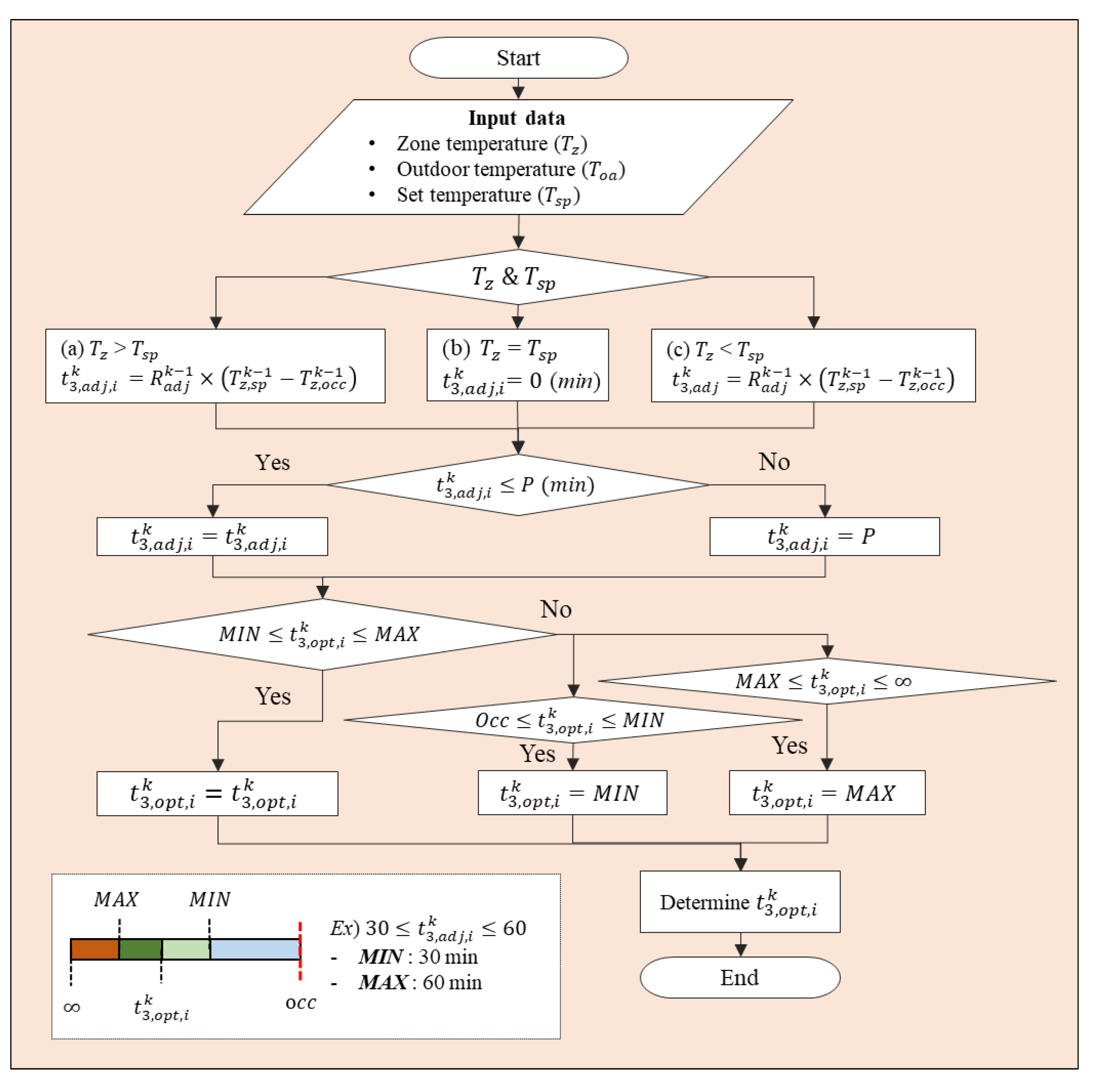
The model 3 is adopted in this paper as it is simple and easy to apply in the field among the three cases. In this model, optimal control is possible and relatively simple if rules are defined for the allowed heating/cooling intervals for over or under operating. According to Figure 1, the data required for optimal control are inputted such as zone temperature (), ambient air temperature (), and set temperature (). First, the component of Equation (7) is calculated and is calculated using and at the occupancy time. adjusts the indoor unit to operate 5 min ( = 5) later when is 1 °C above , while the indoor unit to be operated 5 min faster when is 1 °C below . In the optimal control strategy, is set to a maximum of 25 min (P = 25 min), which is a user-defined value where P is the maximum adjustment time set by the user.
In this study, all values are set at 24 °C, which is a comfortable temperature for the winter, and an optimal control method is necessary to compare a conventional control method to establish an appropriate strategy. In conventional methods, all devices are made to operate before the occupancy time by 60 min. However, different indoor capacity occurs with different temperature increases, resulting in energy waste and both over-heating and under-heating. To address these problems, the control rules proposed in this study suggest maximum and minimum operating boundaries. The maximum operating time (MAX) is set to 60 min for energy saving and the minimum operating time (min) is set to 30 min to reach the set points. If , which is higher than , is created under an operating time of 60 min using this control strategy, is reduced and the system operates for 60 min, but if is low, a maximum of 60 min is maintained to save energy. In addition, is controlled using the rules shown in Figure 1 if a situation occurs outside the maximum and minimum operating conditions. The calculated is used as it is when is within the interval (between MAX and MIN), but if a value greater than the maximum operation is calculated, it is limited by MAX. Conversely, if is lower than the minimum boundary, it is limited by the minimum operating boundary value. MAX shall be set in consideration of energy savings, and min shall be set in consideration of comfort. These boundaries can change depending on the application site by user; in this study, the operating boundaries are empirically set according to the local climate environment and zones in Gwang-ju, South Korea.
2.5. Energy Savings
Energy saving index is usually used to compare amount of the energy consumption between reference use and proposed use [30,31]. In this study, the potential energy savings can be expressed as the ratio of energy use under the optimal method start control to energy use under conventional methods, as shown in Equation (11). The conventional methods are programmed to start VRF systems early enough so that the building will warm up or cool down fast enough on the worst-case morning. As a result, for all other days of the year, the VRF system starts earlier than needed. For the conventional control, the VRF systems are switched on 60 min before the building is occupied in the morning.
where, represents the potential energy saving rate (%); (kWh) is the energy usage under the optimal control strategy; and (kWh) is the energy usage under the conventional control strategy. This study is interested in electricity usage before the schedule, therefore, the electrical usage of the conventional method is set for an hour to facilitate analysis. Accordingly, it is assessed whether energy savings are achieved with the indoor temperature approaching the , comparing power usage over an hour.
3. System Specification and Test Conditions
This chapter briefly introduces the building information and provides schematics of the internal layout in which the optimal control strategy will be applied. Then, a description of the methods used to acquire and analyze data is given so that the reader understands the process. In addition, the points to be considered during the morning hours of interest are described in detail in this paper.
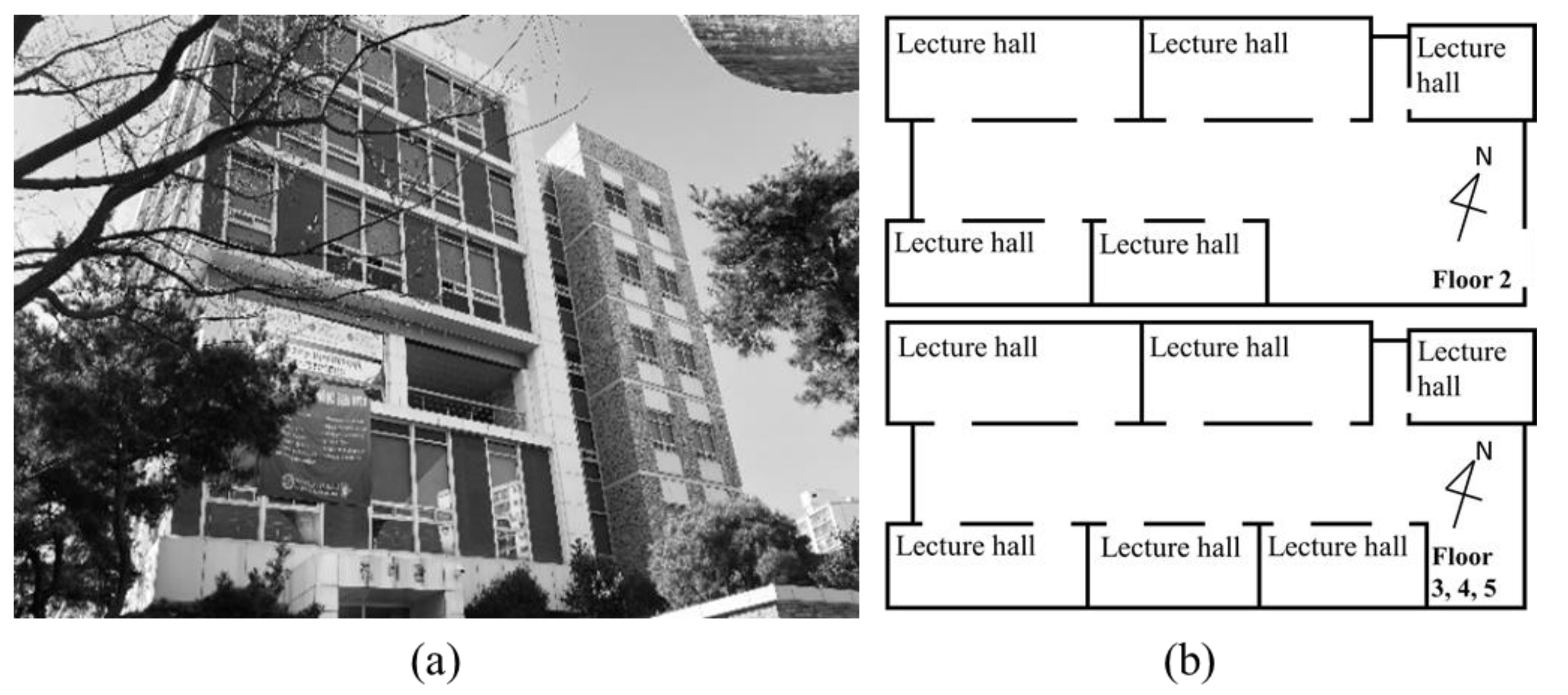
In this section, the process of on-site data acquisition is described in detail. Because on-site data are acquired through experiments rather than simulations, local characteristics are accurately reflected, making it suitable for application of the data-based model that is applied in this study. In other words, data are obtained from the building shown in Figure 2. The demonstration site is a seven-story building located at Chonnam National University in Korea; experiments were conducted using the lecture halls on floor 2 and floor 4. The operation of the indoor units installed in the corridor is excluded. The lecture halls in the building are laid out as shown in Figure 2b, and the cooling/heating schedules depend on the class schedule during the semester. However, in this study, the zone is defined as the area for which the indoor units are responsible, and whether the lecture halls are properly cooled/heated is of primary interest. The heating/cooling facilities installed in the building are all equipped with temperature sensors, which can be used to gauge the temperature change in the specific area. is measured in real-time and reflects the effects of doors, insulation, windows, etc., so the conditions are sufficient to apply the data-based model followed by the optimal control strategy.
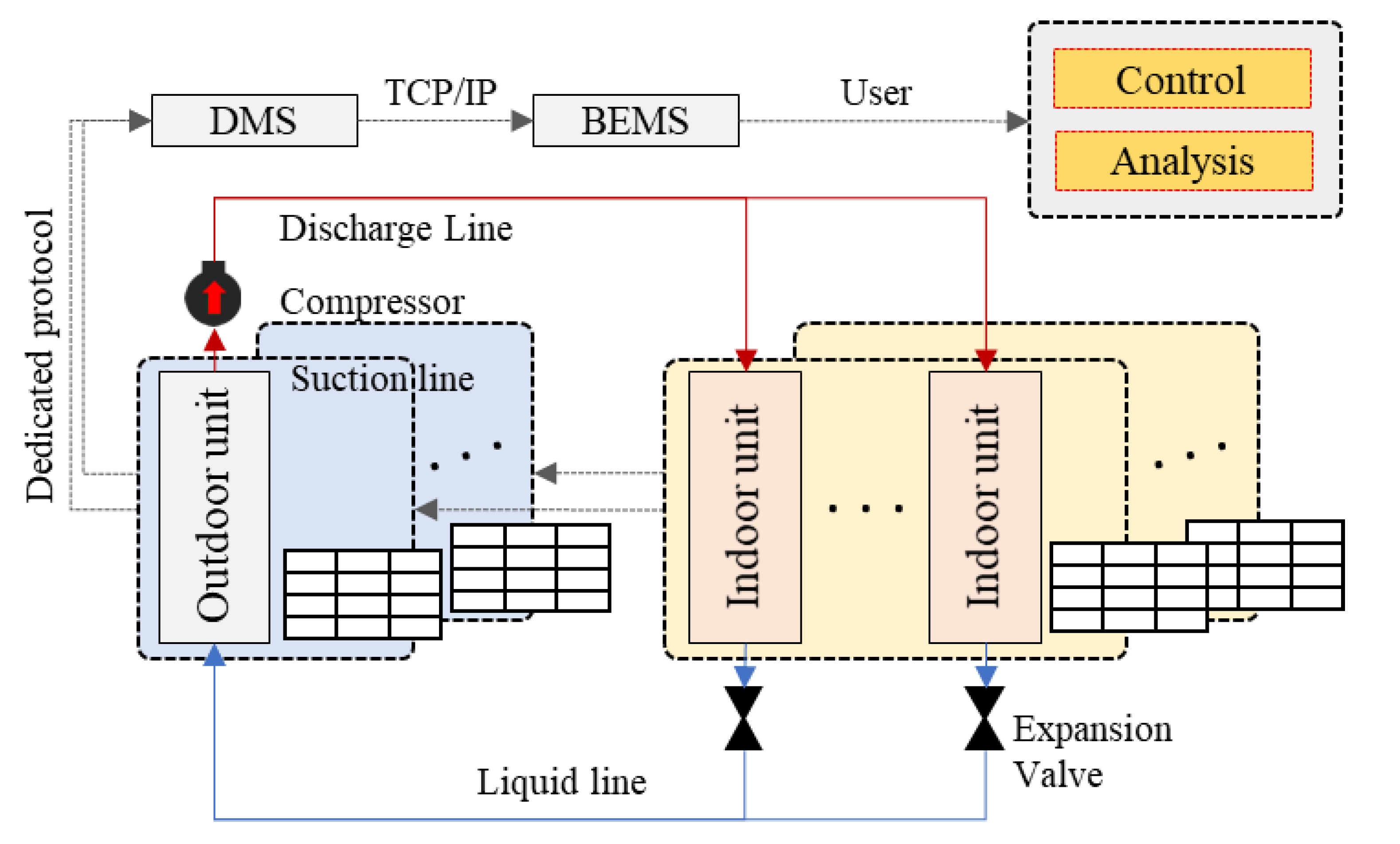
Figure 3 shows that a number of indoor units are connected to one outdoor unit and data are collected in real time, then stored in the data management system (DMS). The working fluid is phase-changed by the compressor and transported by the pump [22]. The red and blue solid lines in Figure 3 indicate the direction in which the working fluid flows, and the cooling/heating mode is controlled by controlling the four-way valve. The zone temperature is measured using a thermostat mounted in the indoor unit on the ceiling. The outdoor temperature is measured in the outdoor unit. In addition, the building energy management system (BEMS), a centralized management system that monitors information in a database using Transmission control protocol and internet protocol (TCP/IP), can control the power, set temperature, and temperature limits of all indoor units from one location. The existing data used in this study were obtained from a DMS system that monitors and writes operational conditions of VRF systems. The DMS system monitors the operational conditions of indoor and outdoor units and writes them to a database at 1-minute intervals. Three different optimal control models were evaluated and validated using two one-week existing datasets from the second weeks of July and January considered to represent a typical summer and winter season as shown in Table 1. The spring/fall dataset was excluded because the VRF systems are not typically running during this period. After the validation of optimal control models using the exiting data, the proposed model was implemented in BEMS. The experiment is performed on VRF systems to enable the evaluation of optimal control. When conducting the experiment, the experiment was carried out by controlling a number of indoor units using BEMS.
The capacity of the outdoor/indoor units installed in the building is detailed in Table 2. The outdoor units 1 and 2 are in charge of cooling/heating on the second floor and outdoor unit 3 is in charge of the fourth floor. According to Table 2, a number of indoor units can be connected without exceeding the capacity of the outdoor unit. Since the outdoor units should be installed in locations where heat discharge will not create problems, all outdoor units are installed on the rooftop of the building. For example, for outdoor unit 1, the heating capacity is 84.9 kW, and zone 1 consists of two indoor units. The control of cooling/heating in spaces such as corridors is not carried out; only lecture hall spaces are climate-controlled. The total heating capacity of the indoor units in zone 1 is 22 kW and the total cooling capacity is 20 kW. One or two indoor units are installed in the lecture halls as shown in Figure 2b. One indoor unit is installed in zone 3, and two indoor units in the others. According to Table 2, zones 1 to 5 correspond to the second floor, indoor units 6 through 8 are installed on the fourth floor. In this study, a strategy is presented to ensure that can be properly controlled depending on the indoor cooling/heating capacity.
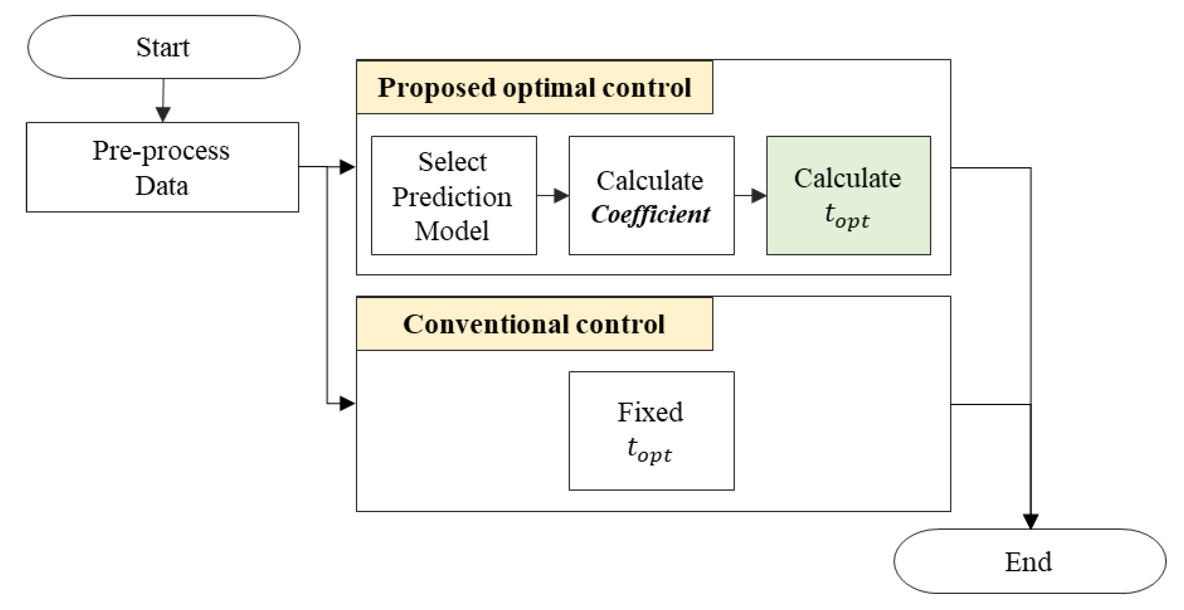
The analysis sequence is examined; conventional and optimal controls are compared with regard to the process of acquiring and analyzing data, as shown in Figure 4. The flowchart in Figure 4 starts with raw data that have not been pre-processed, which in this study are data acquired from the BEMS database. The data reflect the characteristics of each zone and are collected through experiments. This means that the data-based model is suitable for application.
Data cleansing is an essential process when assessing the performance of a model, and incomplete data cleansing can undermine the accuracy of the model because relationships between variables can be distorted. Thus, in this study, missing values and anomalies were removed when data cleansing was performed and the data delay was correctly adjusted. Both physics-and data-based models can be used for conventional control methods. However, in conventional methods, all units are programmed to turn on at the same time and perform pre-cooling. In such cases, energy savings are often not achieved, and even if energy savings are realized, an appropriate comfort level may not be achieved. This can cause problems, so it would ideally be possible to determine the optimal start time according to the unique climate and environment in each zone. For example, although the areas covered by each indoor unit differ, it may be the case that all pre-cooling starts at the same time and the temperature in certain zones may not reach the set points on schedule. Conversely, there are situations in which the capacity is adequate but the system has been operating for a long period of time and too much energy has been supplied. In the proposed optimal control method, a data-based model is used, with coefficients calculated to reflect the thermal characteristics of each zone. In general, when the zone temperature rises, the operation time is used to determine the coefficient of zones. Ultimately, the optimal start time () can be calculated with the aim of maintaining comfort while saving energy before the day’s schedule begins.
4. Results and Discussion
This chapter introduces the results of model prediction accuracy. Then, the proposed optimal control strategy is used to save energy. The performance of the optimal control algorithm is evaluated using the energy saving index in Section 4.2.
4.1. Results of Model Prediction Accuracy
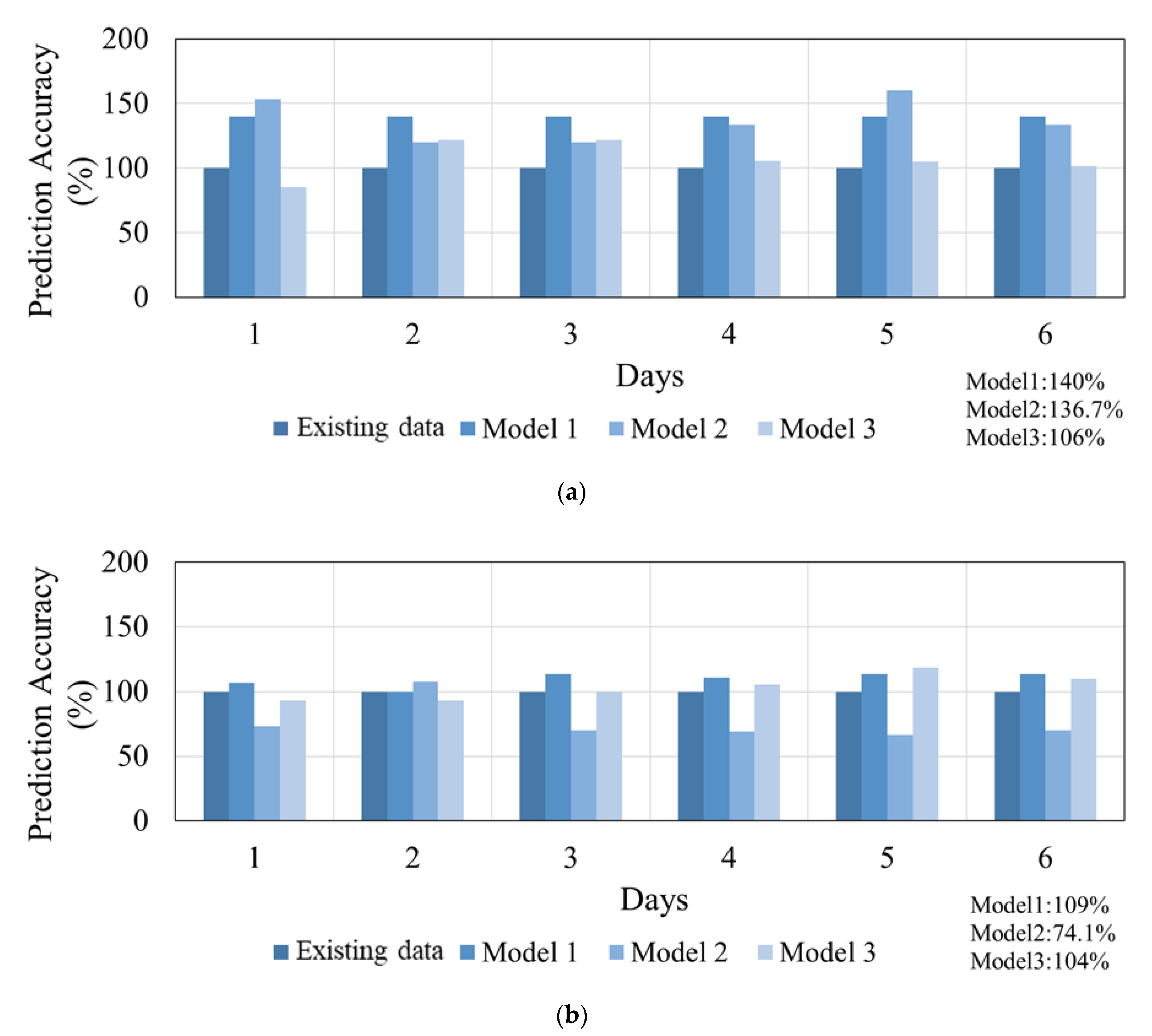
This section presents the analysis results used to select the model with the highest predictive performance, as discussed in Section 2 and Section 3. The predicted performance of the three models is compared using existing summer and winter data (6 days) and the results are shown in Figure 5. The darkest bar represents the time taken from the operating start point to and provides a baseline for the predicted performance among the models. The 100% in the results means that the darkest bars and prediction bars are, at the same time, required to reach the set point. Below 100% means less time is required to reach the set point, but this means less predictive performance because it results in a cold area. For the model 3, the time taken to reach was measured; it showed, on average, a 4% difference from the baseline in summer and 6% in winter. In other words, in both summer and winter, the system is predicted to work longer than the experiment value up to . The model 1 was unable to produce optimal start time calculations due to the large impact of fixed adjustment time, as seen in Section 2.1. The results revealed a fixed tendency for cooling/heating. This means that the adjustment values will not change even if the environment changes. This indicates that model 1 is not flexible in responding to changes in the external environment although all zones have different thermal characteristics. The model 2 can be used to control the heating capacity to provide optimal control. The cooling/heating capacity per hour is required to calculate , so it is difficult to apply unless the facility is suited for such control methods meaning that additional facility costs may be incurred. Given the results shown in Figure 5, will be reached more slowly than the baseline in the summer, and the model 2 predicts that the system will operate for a shorter period of time in winter compared to the baseline values. This shows that Equation (5) is insensitive to changes in the environment. Therefore, in this section, the model 3 is chosen as it produces an output that is most similar to the darkest bar, thus it is used to develop the optimal control rules.
4.2. Results of the Proposed Optimal Strategy
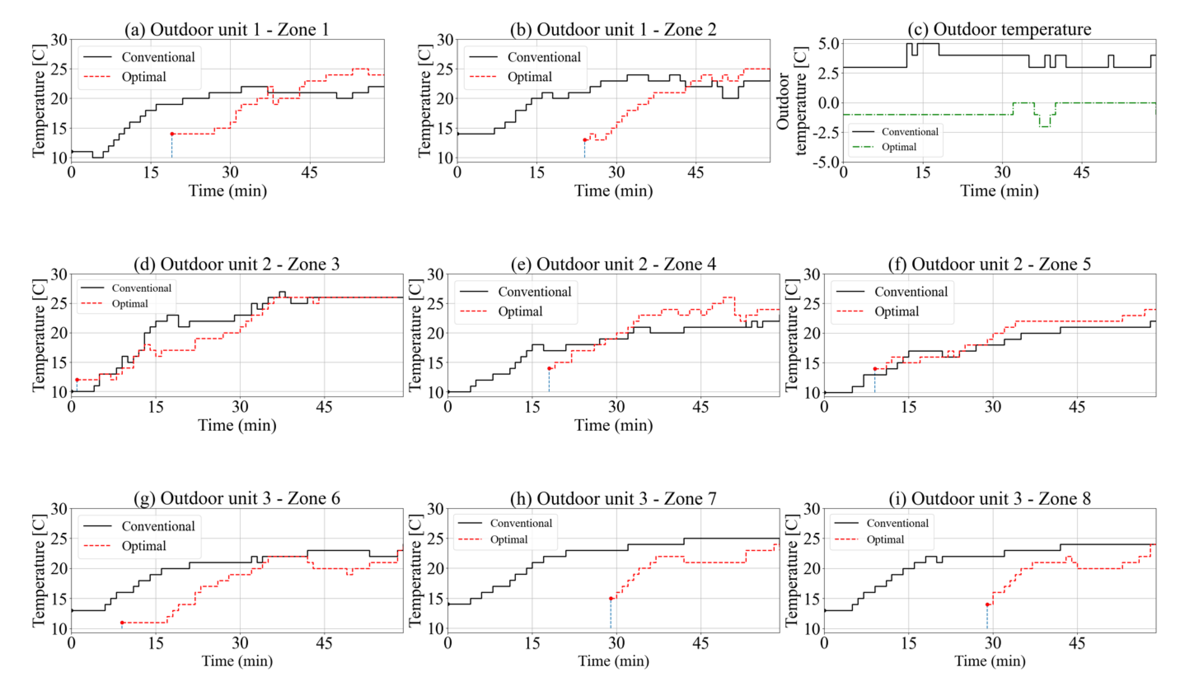
Use of the conventional controls ensures that all of the indoor unit power is on at the same time, as illustrated in Figure 4. In this paper, indoor units operate during an hour when conventional control is applied as the one-hour operation is to facilitate analysis of power usage. The experiment was conducted during the third week of January 2020 and it was not conducted on weekends. The in all zones is 24 °C and the air supply flow rate into all zones is the same. In all areas, generally increases during the first half hour, and energy is continuously used to maintain the temperature for the next half hour in case of the conventional control method. In other words, conventional control wastes energy because it operates indoor units more than necessary. The results from the experiment are shown in Table 3. In this section, the performance of the optimal control strategy is verified through the results of two cases: the day when energy saving is best and the day when it is lowest. Day 4 of Table 3 shows the worst energy saving case in Figure 6. Day 5 of Table 3 shows the best energy saving in Figure 7.
According to the lowest energy saving case (day 4), zone 3 is equipped with indoor unit 3 (Figure 6), and it is the smallest lecture hall on the second floor in Figure 1. The outdoor temperature profile is presented in Figure 6c to verify to calculate using the model 3. cannot be controllable. The optimal control model is affected by in Figure 6c. Indoor units of (a) to (i) are turned on between 8:01 a.m. and 8:29 a.m. because proper optimal starting points are determined by calculating . The was −1 °C on day 4, and the was distributed between the lowest 11 °C and the highest 15 °C. The results of the optimal start calculation were applied to each zone, reaching and average of about 24.1 °C. This result means that the average operating time was reduced by about 17 min using optimal control strategy. Figure 6d shows that zone 3 takes more than 30 min to reach 24 °C but continues to waste electricity to maintain that temperature once it is reached. This excess results in wasted energy suggesting that operating in more than one building rather than a single zone can lead to serious energy waste. In that case, it is difficult to maintain a comfortable temperature. In this paper, the optimal control rule as defined in chapter 2.4 is applied to solve the problem of energy waste. For the conventional control in Figure 6, the at 24 °C may have resulted in an indoor temperature that is either too high or too low due to environmental effects. However, the energy is wasted to maintain the temperature if the temperature reaches 24 °C before that time, considering that the scheduled start time is 9 a.m. To solve these problems, the data from a day before were used to determine the start time. For example, indoor units operate about 10 to 20 min later than the conventional strategy, but it may produce the close to the , with the predicted time shown in Figure 6. The results are used to create a forecast for the following day. If is 2 °C higher than , will be adjusted so that the indoor unit turns on 10 min later the next day. Conversely, the results in Figure 6h shows that the value is 23 °C, so the is adjusted to turn the unit on 5 min earlier the next day. Overall, the approached the closely while saving energy. Overall, the optimal control can reduce the energy consumption by keeping a facility in its unoccupied mode for as long as possible and putting it in unoccupied mode as soon as possible without sacrificing comfort.
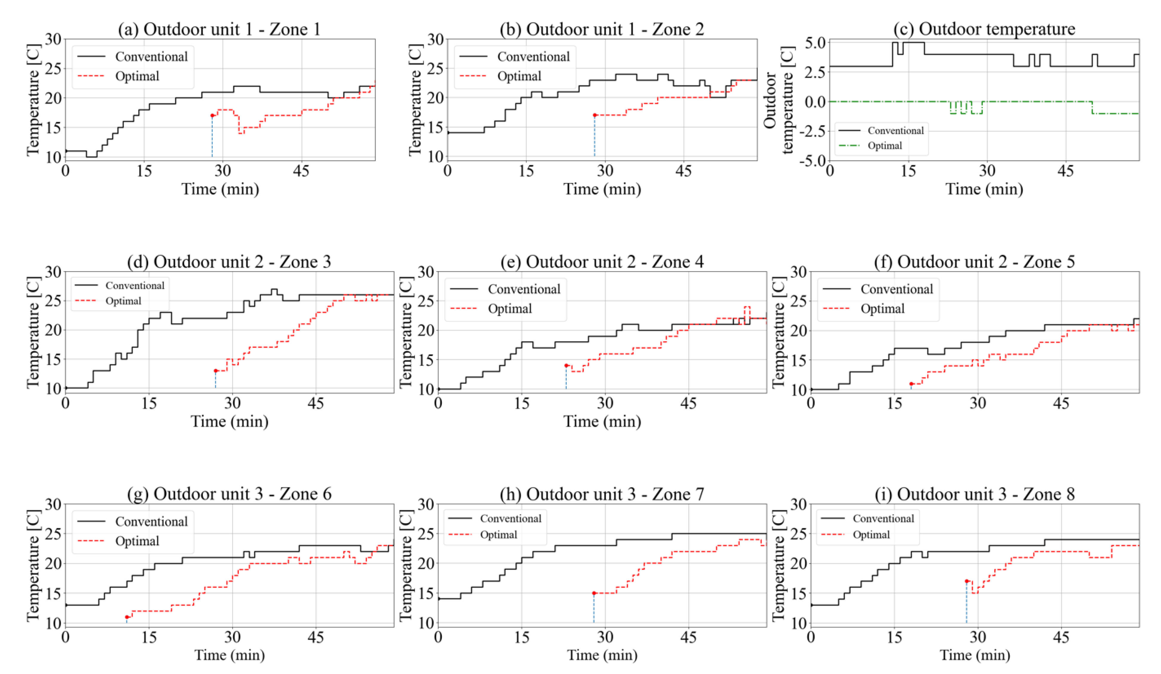
According to the highest energy saving case, excessive indoor temperature results were not derived before the occupancy time, except in zone 3. The outdoor temperature profile is presented in Figure 7c to verify to calculate using the model 3. The cannot be controllable. The indoor units of (a) to (i) are turned on between 8:11 a.m. and 8:28 a.m. because proper optimal starting points are determined by calculating . The was −1 °C on day 5, and the was distributed between the lowest 11 °C and the highest 17 °C. The results of the optimal start calculation were applied to each zone, reaching and average of about 23 °C. Comparing with a result of zone 3 in Figure 6 (day 4), the indoor unit 3 operates from 8:27 a.m. Then, the of zone 3 reaches the at about 8:50 a.m. and subsequent energy use is to be considered wasted. Given the results, the average operating time was reduced by about 23 min on average using the optimal control strategy. Specifically, an optimal start algorithm can reduce the time waste by about 15 min to maintain the in case of zone 3 as shown in Figure 7 (day 5). This means that operating in more than one building rather than a single zone can save serious energy waste. The results of other zones are similar, but it should be considered that waste can occur because of various causes such that is not the same every day. The waste by environmental variables is adjusted by calculating . So, can be corrected using and applied the next day. This suggests that the proposed control algorithm can make zones comfortable while saving energy. As the operating durations decrease, the amount of the energy use is also reduced, which increases the energy saving rate; the larger the size of the application site, the greater the energy saving can be.
The results shown in Figure 6 and Figure 7 demonstrate that zone-specific control is possible, and Figure 8 can be used to examine the potential energy savings in terms of outdoor units. Figure 8a shows the results of day 4 and Figure 8b shows the results of day 5. The energy usage was measured with an energy meter and data were recorded every 15 min for each outdoor unit. The outdoor unit 1 is recorded by summing the power consumption used in zones 1 to 2 of Figure 6. The outdoor unit 2 is recorded by summing the energy usage in zones 3 to 5. The outdoor unit 3 is recorded by summing the electricity used in zones 6 to 8. For example, the energy saving of the outdoor unit 1 is 33.3% on day 4 and 49.0% on day 5. The energy saving of the outdoor unit 2 is 12.5% on day 4 and 36.1% on day 5. The energy saving of the outdoor unit 3 is 16.9% on day 4 and 37.5% on day 5. This experiment resulted in an average energy saving of 20.9% on day 4 and 40.9% on day 5. Based on these results, the optimal control strategy can reduce the amount of electricity used by each outdoor unit by controlling energy use by each indoor unit.
The experiment was conducted over a total of five days and the energy saving was calculated using Equation (11). The amount of energy used was determined only for an hour because it is assumed that all indoor units run at the same time at 8 a.m. and this study is only interested in the time before the beginning of the schedule. The results shown in Table 4 were recorded on five consecutive weekdays; the experiment was not conducted on the weekend. Daily average power consumption and total average are displayed in Table 4. During the five experimental days, an average energy saving of 30.5% was achieved.
5. Conclusions
In this study, optimal control strategies were developed using data collected at a building site to facilitate energy saving. The existing data were used to evaluate predictive accuracy among three data-based models. In order to develop a successful optimal control algorithm, an investigation was conducted about the environment such as the building information and the location of units. Then, the mechanism of the VRF system and the overall data acquisition process were described. Three data-based models were presented to compensate for the degradation performance of the physics-based model and to improve on-site applicability. The and are used to calculate in the first model. However, the first model does not allow for flexible control because it has a fixed minimum operating time. For calculating , rated capacity are used in the second model. The second model is easy to apply when optimal control is performed via control of the heating capacity but requires a facility capable of reacting sensitively to environmental changes. The , and are used to calculate in the third model. The third model uses and to correct the predicted time and perform optimal control through simple on/off control. Thus, the third model, which showed the highest predictive performance, was selected in this paper. The selected model was used to develop the optimal control strategy. In addition, the optimal control rules were presented in detail. The experiments were conducted to assess the performance of the optimal control strategy during the third week of 2020. The experimental results were used to compare the conventional vs. optimal control strategy; performance was compared between the two, and the temperature curve confirmed that the time required for temperature rise was accurately predicted. In general, the use of an optimal control strategy reduces the amount of energy required to maintain the air temperature after a temperature increase, and the system can be controlled to accurately reach the at the time of occupancy, which is not the case under a conventional control strategy. In addition, the performance of the optimal control algorithm was evaluated by calculating the energy savings for each outdoor unit after experiments are conducted on site. The analysis of energy savings using all outdoor units showed an average energy saving of 30.5%. Based on these results, an optimal control strategy was developed to save energy and make users more comfortable during the occupancy time.
Author Contributions
Conceptualization, Y.L. and W.K.; methodology, Y.L. and W.K.; software, Y.L.; validation, Y.L.; formal analysis, Y.L.; investigation, Y.L.; resources, Y.L.; data curation, Y.L.; writing—original draft preparation, Y.L.; writing—review and editing, Y.L. and W.K.; visualization, Y.L.; supervision, W.K.; project administration, W.K.; funding acquisition, W.K. All authors have read and agreed to the published version of the manuscript.
Funding
This research was supported by the Basic Science Research Program through the National Research Foundation of Korea (NRF) funded by the Ministry of Education (2019R1G1A1100470).
Data Availability Statement
Data sharing not applicable.
Conflicts of Interest
The authors declare no conflict of interest.
Nomenclature
| Coefficient at which the zone heats up after equipment start-up | |
| Adjustment of heating capacity | |
| Coefficient of temperature response | |
| Coefficient of heating transfer | |
| Energy saving (%) | |
| Energy usage (kWh) | |
| Min-operating time (min) | |
| Max-operating time (min) | |
| Maximum adjustment time (min) | |
| Adjustment weight (min/) | |
| Time (min) | |
| Temperature () | |
| Subscripts | |
| Adjust | |
| Conventional | |
| Initial | |
| Zone number | |
| Day number | |
| Occupancy time | |
| Optimal | |
| Outdoor air | |
| Rated | |
| Set point (set) | |
References
- Burnard, K.; Bhattacharya, S. Power Generation from Coal-Ongoing Developments and Outlooks; International Energy Agency: Paris, France, 2011. [Google Scholar]
- Kapusta, K.; Stańczyk, K. Pollution of water during underground coal gasification of hard coal and lignite. Fuel 2011, 90, 1927–1934. [Google Scholar] [CrossRef]
- Liu, M.; Claridge, D.E.; Turner, W.D. Continuous commissioningSM of building energy systems. J. Sol. Energy Eng. 2003, 125, 275–281. [Google Scholar] [CrossRef]
- Mills, E. Building commissioning: A golden opportunity for reducing energy costs and greenhouse gas emissions in the United States. Energy Effic. 2011, 4, 145–173. [Google Scholar] [CrossRef] [Green Version]
- Sun, Y.; Wang, S.; Huang, G. Model-based optimal start control strategy for multi-chiller plants in commercial buildings. Build. Serv. Eng. Res. Technol. 2010, 31, 113–129. [Google Scholar]
- Yang, I.-H. Development of an artificial neural network model to predict the optimal pre-cooling time in office buildings. J. Asian Arch. Build. Eng. 2010, 9, 539–546. [Google Scholar] [CrossRef]
- Xu, B.; Zhou, S.; Hu, W. An intermittent heating strategy by predicting warm-up time for office buildings in Beijing. Energy Build. 2017, 155, 35–42. [Google Scholar] [CrossRef]
- Gayeski, N.T.; Armstrong, P.R.; Norford, L.K. Predictive pre-cooling of thermo-active building systems with low-lift chillers. HVAC&R Res. 2012, 18, 1–16. [Google Scholar]
- Motegi, N.; Piette, M.A.; Watson, D.S.; Kiliccote, S.; Xu, P. Introduction to Commercial Building Control Strategies and Techniques for Demand Response—Appendices; No. LBNL-59975; Lawrence Berkeley National Laboratory (LBNL): Berkeley, CA, USA, 2007. [Google Scholar]
- Zhao, P.; Suryanarayanan, S.; Simoes, M.G. An energy management system for building structures using a multi-agent decision-making control methodology. IEEE Trans. Ind. Appl. 2013, 49, 322–330. [Google Scholar] [CrossRef]
- Yin, R.; Xu, P.; Piette, M.A.; Kiliccote, S. Study on Auto-DR and pre-cooling of commercial buildings with thermal mass in California. Energy Build. 2010, 42, 967–975. [Google Scholar] [CrossRef] [Green Version]
- Prívara, S.; Široký, J.; Ferkl, L.; Cigler, J. Model predictive control of a building heating system: The first experience. Energy Build. 2011, 43, 564–572. [Google Scholar] [CrossRef]
- Alcalá, R.; Benítez, J.M.; Casillas, J.; Cordón, O.; Pérez, R. Fuzzy control of HVAC systems optimized by genetic algorithms. Appl. Intell. 2003, 18, 155–177. [Google Scholar] [CrossRef]
- Hilliard, T.; Swan, L.; Qin, Z. Experimental implementation of whole building MPC with zone based thermal comfort adjustments. Build. Environ. 2017, 125, 326–338. [Google Scholar] [CrossRef]
- Kummert, M.; André, P.; Nicolas, J. Building and HVAC optimal control simulation. Application to an office building. In Proceedings of the Third International Symposium on HVAC; Tsinghua University: Beijing, China; Hong Kong Polytechnical University: Hong Kong, China, 1999; pp. 857–868. [Google Scholar]
- Chen, C.; Wang, J.; Heo, Y.; Kishore, S. MPC-based appliance scheduling for residential building energy management controller. IEEE Trans. Smart Grid 2013, 4, 1401–1410. [Google Scholar] [CrossRef]
- Lim, B.; Hijazi, H.; Thiébaux, S.; Briel, M.V.D. Online HVAC-aware occupancy scheduling with adaptive temperature control. In Principles and Practice of Constraint Programming; Springer International Publishing: New York, NY, USA, 2016; Volume 9892, pp. 683–700. [Google Scholar]
- Xu, P.; Haves, P.; Piette, M.A.; Braun, J. Peak Demand Reduction from Pre-Cooling with Zone Temperature Reset in an Office Building; Lawrence Berkeley National Laboratory: Berkeley, CA, USA, 2004. [Google Scholar]
- Nikovski, D.; Xu, J.; Nonaka, M. A method for computing optimal set-point schedules for HVAC systems. In Proceedings of the 11th REHVA World Congress CLIMA, Prague, Czech Republic, 16–19 June 2013. [Google Scholar]
- Afram, A.; Janabi-Sharifi, F. Black-box modeling of residential HVAC system and comparison of gray-box and black-box modeling methods. Energy Build. 2015, 94, 121–149. [Google Scholar] [CrossRef]
- Muratori, M.; Marano, V.; Sioshansi, R.; Rizzoni, G. Energy consumption of residential HVAC systems: A simple physically-based model. In Proceedings of the 2012 IEEE Power and Energy Society General Meeting, San Diego, CA, USA, 22–26 July 2012; Institute of Electrical and Electronics Engineers (IEEE): New York, NY, USA, 2012; pp. 1–8. [Google Scholar]
- Tang, R.; Wang, S.; Shan, K.; Cheung, H. Optimal control strategy of central air-conditioning systems of buildings at morning start period for enhanced energy efficiency and peak demand limiting. Energy 2018, 151, 771–781. [Google Scholar] [CrossRef]
- Park, B.R.; Yang, Y.K.; Hong, J.; Lee, J.H.; Moon, J.W. Development of an energy cost prediction model for a VRF heating system. Appl. Therm. Eng. 2018, 140, 476–486. [Google Scholar] [CrossRef]
- Liu, J.; Hu, Y.; Chen, H.; Wang, J.; Li, G.; Hu, W. A refrigerant charge fault detection method for variable refrigerant flow (VRF) air-conditioning systems. Appl. Therm. Eng. 2016, 107, 284–293. [Google Scholar] [CrossRef]
- Perez, K.X.; Baldea, M.; Edgar, T.F. Integrated HVAC management and optimal scheduling of smart appliances for community peak load reduction. Energy Build. 2016, 123, 34–40. [Google Scholar] [CrossRef] [Green Version]
- Mossolly, M.; Ghali, K.; Ghaddar, N. Optimal control strategy for a multi-zone air conditioning system using a genetic algorithm. Energy 2009, 34, 58–66. [Google Scholar] [CrossRef]
- Zajic, I.; Larkowski, T.; Sumislawska, M.; Burnham, K.; Hill, D. Modelling of an air handling unit: A Hammerstein-bilinear model identification approach. In Proceedings of the 2011 21st International Conference on Systems Engineering, Las Vegas, NV, USA, 16–18 August 2011; Institute of Electrical and Electronics Engineers (IEEE): New York, NY, USA, 2011; pp. 59–63. [Google Scholar]
- Hilliard, T.; Swan, L. A tool for evaluating the performance of simplified models for predictive control applications. In Proceedings of the 15th IBPSA Conference, San Francisco, CA, USA, 7–9 August 2017; pp. 672–681. [Google Scholar]
- Moon, J.W.; Yang, Y.K.; Choi, Y.J.; Lee, K.-H.; Kim, Y.-S.; Park, B.R. Development of a control algorithm aiming at cost-effective operation of a VRF heating system. Appl. Therm. Eng. 2019, 149, 1522–1531. [Google Scholar] [CrossRef]
- Ye, H.; Long, L.; Zhang, H.; Gao, Y. The energy saving index and the performance evaluation of thermochromic windows in passive buildings. Renew. Energy 2014, 66, 215–221. [Google Scholar] [CrossRef]
- Bakar, N.N.A.; Hassan, M.Y.; Abdullah, H.; Rahman, H.A.; Abdoullah, M.P.; Hussin, F.; Bandi, M. Energy efficiency index as an indicator for measuring building energy performance: A review. Renew. Sustain. Energy Rev. 2015, 44, 1–11. [Google Scholar] [CrossRef]
Figure 1.
Optimal control strategy and rules.

Figure 2.
(a) Building used for demonstration, (b) layout of the building.

Figure 3.
On-site data acquisition process.

Figure 4.
Comparison of the proposed optimal and conventional control strategies.

Figure 5.
Prediction accuracy from outdoor units using existing data. (a) Comparison of prediction accuracy in summer; (b) comparison of prediction accuracy in winter.
Figure 5.
Prediction accuracy from outdoor units using existing data. (a) Comparison of prediction accuracy in summer; (b) comparison of prediction accuracy in winter.

Figure 6.
Comparison of the optimal control effect by indoor and outdoor units (day 4): (a,b) outdoor unit 1, (c) outdoor temperature, (d–f) outdoor unit 2, (g–i) outdoor unit 3.
Figure 6.
Comparison of the optimal control effect by indoor and outdoor units (day 4): (a,b) outdoor unit 1, (c) outdoor temperature, (d–f) outdoor unit 2, (g–i) outdoor unit 3.

Figure 7.
Comparison of the optimal control effect by indoor and outdoor units (day 5): (a,b) outdoor unit 1, (c) outdoor temperature, (d–f) outdoor unit 2, (g–i) outdoor unit 3.
Figure 7.
Comparison of the optimal control effect by indoor and outdoor units (day 5): (a,b) outdoor unit 1, (c) outdoor temperature, (d–f) outdoor unit 2, (g–i) outdoor unit 3.

Figure 8.
Energy savings with the optimal control strategy. (a) Comparison between conventional and optimal control (day 4); (b) comparison between conventional and optimal control (day 5).
Figure 8.
Energy savings with the optimal control strategy. (a) Comparison between conventional and optimal control (day 4); (b) comparison between conventional and optimal control (day 5).


Table 1.
Existing data and experiments.
| Purpose | Periods | |
|---|---|---|
| Existing data | The comparison of prediction performance among the models | 2nd week of July 2019 2nd week of January 2019 |
| Experiments | Validation of the optimal start strategy performance | 3rd week of January 2020 |
Table 2.
Cooling and heating capacity of outdoor/indoor units.
| Outdoor Units | Outdoor Unit Capacity (kW) | Zone Number | Indoor Unit Capacity (kW) | ||
|---|---|---|---|---|---|
| Heating | Cooling | Heating | Cooling | ||
| 1 | 84.9 | 75.4 | 1 | 22 | 20 |
| 2 | 22 | 20 | |||
| 2 | 84.9 | 75.4 | 3 | 14.5 | 13 |
| 4 | 32.6 | 29 | |||
| 5 | 32.6 | 29 | |||
| 3 | 104.4 | 92.8 | 6 | 22 | 20 |
| 7 | 22 | 20 | |||
| 8 | 22 | 20 | |||
Table 3.
Experimental results of optimal start time.
| Outdoor Units | 1 | 2 | 3 | ||||||
|---|---|---|---|---|---|---|---|---|---|
| Zone | 1 | 2 | 3 | 4 | 5 | 6 | 7 | 8 | |
| Heating Capacity (kW) | 22 | 22 | 14.5 | 32.6 | 32.6 | 22 | 22 | 22 | |
| Day 1 | Tz,init | 17 | 17 | 10 | 11 | 8 | 10 | 10 | 10 |
| Tz,occ | 22 | 22 | 24 | 21 | 21 | 20 | 23 | 22 | |
| Toa | −3 | ||||||||
| 8:30 | 8:30 | 8:22 | 8:16 | 8:10 | 8:13 | 8:19 | 8:25 | ||
| Day 2 | Tz,init | 10 | 13 | 13 | 12 | 8 | 10 | 12 | 13 |
| Tz,occ | 23 | 24 | 26 | 23 | 22 | 23 | 25 | 26 | |
| Toa | 0 | ||||||||
| 8:30 | 8:30 | 8:09 | 8:12 | 8:02 | 8:00 | 8:09 | 8:09 | ||
| Day 3 | Tz,init | 9 | 12 | 15 | 12 | 8 | 10 | 12 | 15 |
| Tz,occ | 24 | 23 | 24 | 21 | 22 | 23 | 25 | 25 | |
| Toa | −2 | ||||||||
| 8:09 | 8:26 | 8:30 | 8:18 | 8:00 | 8:17 | 8:28 | 8:30 | ||
| Day 4 | Tz,init | 14 | 13 | 12 | 14 | 15 | 11 | 15 | 14 |
| Tz,occ | 24 | 25 | 25 | 24 | 24 | 24 | 23 | 24 | |
| Toa | −1 | ||||||||
| 8:19 | 8:24 | 8:01 | 8:18 | 8:09 | 8:09 | 8:29 | 8:29 | ||
| Day 5 | Tz,init | 17 | 17 | 13 | 14 | 11 | 11 | 16 | 17 |
| Tz,occ | 23 | 23 | 26 | 21 | 21 | 23 | 24 | 23 | |
| Toa | −1 | ||||||||
| 8:28 | 8:28 | 8:27 | 8:23 | 8:18 | 8:11 | 8:28 | 8:28 | ||
Table 4.
Daily and average energy savings.
| Energy Saving (%) | Outdoor Unit 1 | Outdoor Unit 2 | Outdoor Unit 3 | Average |
|---|---|---|---|---|
| Day 1 | 50.0% | 24.4% | 31.6% | 35.3% |
| Day 2 | 50.0% | 10.9% | 10.0% | 23.6% |
| Day 3 | 32.2% | 21.4% | 41.7% | 31.8% |
| Day 4 | 33.3% | 12.5% | 16.9% | 20.9% |
| Day 5 | 49.0% | 36.1% | 37.5% | 40.9% |
| Average | 42.9% | 21.1% | 27.5% | 30.5% |
Publisher’s Note: MDPI stays neutral with regard to jurisdictional claims in published maps and institutional affiliations. |
© 2021 by the authors. Licensee MDPI, Basel, Switzerland. This article is an open access article distributed under the terms and conditions of the Creative Commons Attribution (CC BY) license (http://creativecommons.org/licenses/by/4.0/).
Share and Cite
MDPI and ACS Style
Lee, Y.; Kim, W. Development of an Optimal Start Control Strategy for a Variable Refrigerant Flow (VRF) System. Energies 2021, 14, 271. https://0-doi-org.brum.beds.ac.uk/10.3390/en14020271
AMA Style
Lee Y, Kim W. Development of an Optimal Start Control Strategy for a Variable Refrigerant Flow (VRF) System. Energies. 2021; 14(2):271. https://0-doi-org.brum.beds.ac.uk/10.3390/en14020271
Chicago/Turabian StyleLee, Yusung, and Woohyun Kim. 2021. "Development of an Optimal Start Control Strategy for a Variable Refrigerant Flow (VRF) System" Energies 14, no. 2: 271. https://0-doi-org.brum.beds.ac.uk/10.3390/en14020271
Note that from the first issue of 2016, this journal uses article numbers instead of page numbers. See further details here.