New Equation for Optimal Insulation Dependency on the Climate for Office Buildings


1
Department of Civil Engineering, School of Engineering, Aalto University, PO Box 12100 FI-00076 Aalto, 02150 Espoo, Finland
2
Granlund Oy, PO Box 59 FI-00701, 00700 Helsinki, Finland
3
Smart City Center of Excellence, Tallinn University of Technology, Ehitajate Tee 5, 19086 Tallinn, Estonia
*
Author to whom correspondence should be addressed.
Energies 2021, 14(2), 321; https://0-doi-org.brum.beds.ac.uk/10.3390/en14020321
Submission received: 10 November 2020
/
Revised: 31 December 2020
/
Accepted: 4 January 2021
/
Published: 8 January 2021
(This article belongs to the Special Issue Energy Performance and Indoor Climate in Buildings)
Abstract
:The comparison of building energy efficiency in different climates is a growing issue. Unique structural solutions will not ensure the same energy use, but the differences also remain if cost-optimal solutions are applied. This study developed a new equation for the assessment of building envelope optimal insulation in different climates for office buildings. The developed method suggests determining actual degree days from simulated heating energy need and the thermal conductance of a building, avoiding in such a way the use of a base temperature. The method was tested in four climates and validated against cost-optimal solutions solved with optimization. The accuracy of the method was assessed with sensitivity analyses of key parameters such as window-to-wall ratios (WWRs), window g-values, costs of heating, and electricity. These results showed that the existing square root equation overestimated the climate difference effect so that the calculation from the cold climate U-value resulted in less insulation than cost-optimal in warmer climates. Parametric analyses revealed that the power value of 0.2 remarkably improved the accuracy as well as performance worked well in all cases and can be recommended as a default value. Sensitivity analyses with a broad range of energy costs and window parameters revealed that the developed equation resulted in maximum 5% underestimation and maximum 7% overestimation of an average area-weighted optimal U-value of building envelope in another climate. The developed method allows objectively to compare optimal insulation of the building envelope in different climates. The method is easy to apply for energy performance comparison of similar buildings in different climates and also for energy performance requirements comparison.
1. Introduction
In the European Union (EU), residential and non-residential buildings account for 75% and 25% of the total building stock, respectively [1]. Office buildings have a significant share of 23% among non-residential buildings stock, which is considered a viable source of energy usages [1]. For instance, the average heating and cooling need of office buildings in the EU are 159 and 7 TWh/year, respectively [2]. Though these are the key sectors of energy use in buildings, significant variations of heating and cooling need are observed when buildings are located in different climates. To fulfil the same thermal comfort and other indoor environmental quality (IEQ) criteria, different outdoor conditions will cause substantial differences in energy demands for heating, cooling, ventilation, and lighting. Thus, the EU defines the benchmark of nearly zero energy building (NZEB) office building for four climate zones [3].
Many scientific research works introduce building parameters and their uncertainties, which have significant impacts on buildings’ energy efficiency [4,5,6]. Eisenhower et al. [4] presented a large number of potential parameters that have a substantial effect on buildings design. Bucking et al. [5] proposed a methodology in which scaling up the different building parameters for improving buildings’ energy efficiency. Besides, this study distinguished the effects of insulation level and window areas on buildings’ energy performance. In the same context, Sun et al. [6] analyzed the uncertainty of microclimatic variables, namely local temperature, solar irradiation, wind speed, and pressure for the energy assessment of buildings. The study showed the fundamental differences in energy consumption due to climatic variations [6].
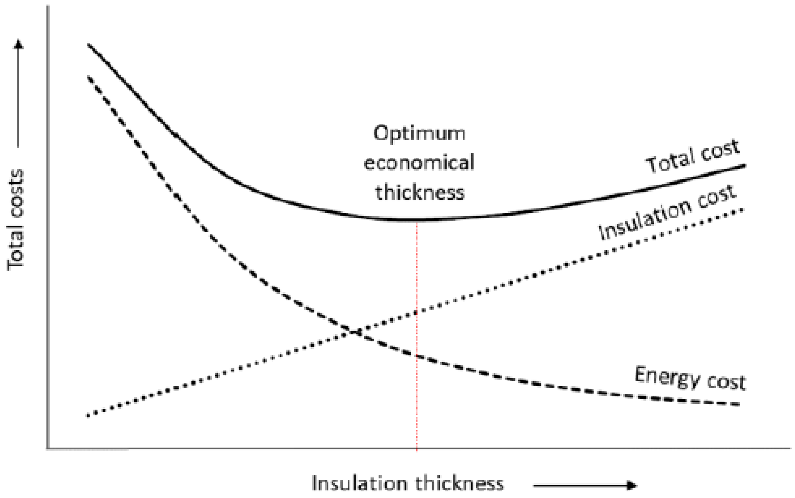
Many scientific articles emphasize the importance of passive solutions such as improving building insulation, windows’ ‘U-value’, and windows’ ‘g value’. However, the insulation level is only one parameter within total performance, typically measured by return on investment, indoor thermal comfort, and achieving NZEB benchmarks. An excessive insulation thickness increases the investment cost and may have some effect on cooling demands during the summer. Kaynakli [7] tabulated parameters such as building type, the efficiency of installed systems, availability of energy sources and cost, etc., to estimate the optimal insulation thickness. The optimal point of insulation thickness based on investment cost and yearly energy-saving potential is shown in Figure 1. The total cost needs to be calculated as a life cycle cost for a specified period because energy costs occur every year. Optimal insulation may be considered as one component within the cost-optimal calculation [8], which also covers technical building systems and energy sources. In a similar context, Ibrahim et al. found the wall orientation dependency on finding the optimal insulation thickness of external walls [9].
The optimum thermal transmittance coefficient of building facade and windows require to ensure the low investment and life cycle cost, improving building energy efficiency that complies with the national NZEB benchmark and a healthy indoor climate condition. Rosti et al. [10] obtained the ideal insulation thickness of the external wall in eight climate zones in Iran. The results were obtained from the numerical solution under dynamic thermal conditions, which acknowledged the energy-saving potentials and payback period. Bolatturk [11] used a life-cycle cost analysis approach, similar to Rosti et al. [10], to find out the optimum insulation thicknesses for four climate zones in Turkey. Beyond these, D’Agostino et al. [12] used the cost-optimal methodology to describe the optimum insulation thickness of an office building for cities of Palermo, Milan, and Cairo. In addition to life cycle cost, optimal insulation may be approached from cooling and environmental aspects as done for several cities and climate zones [7,13,14,15].
All these studies have not explicitly accounted for window properties and the window-to-wall ratio (WWR) in annual energy needs while proposing optimal insulation thickness. So far, very few studies have acknowledged the effects of windows properties and window to wall ratio while demonstrating the cost-optimal solution. Such combined effects seem substantial, as studies have shown variation in the optimal solution of wall insulation for different glazing types and areas [15,16,17,18,19]. Thalfeldt et al. determined the cost-optimal facade solution for the Estonian climate [18]. The results showed the promotion of energy efficiency of a building by improving the U-value of windows, low emissivity coating, and daylight considering a selection of WWRs. In a similar context, Pikas et al. proposed a fenestration design solution for an Estonian office building. This study concluded that a small window-to-wall ratio and an insulation thickness of 0.2 m were the most cost-optimal solution for the Estonian climate [19].
In the optimum insulation analyses, many researchers have used the degree days method to estimate energy needs [11,13,20]. The degree days method considers the steady-state condition, and it is related to the climate variable of air temperature only. The main drawback of the degree days method that it assumes the energy need being proportional to the difference between outdoor air and the base temperature. The base temperature requires taking into account the effect of the dynamic behavior of weather, internal and solar heat gains, and thermal mass; otherwise, it could lead to considerable errors of heating need and optimal insulation thickness solution [21]. In the same context, Harvey [22] found a limitation of the heating degree day (HDD) method, which could not estimate the heating demand accurately because of it accounting for daily balance point temperatures. Similarly, cooling load is poorly estimated by using the degree days approach due to ignoring the solar radiations and internal heat gains [23]. However, degree days still may be used as a climate variable if the transient behaviors are taken into account in an energy simulation [24,25,26]. Ahmed et al. [26] applied a dynamic energy simulation for a reference office building in which heating, cooling, and lighting needs were analyzed in four climates. While economic insulation thickness was known in one climate, it was possible to calculate economic insulation with Equation (1) in other climates, enabling one to compare the buildings or energy performance requirements in different countries.
where, is optimal thermal transmittance of the respective building for a reference climate (W/m2K), is the optimal thermal transmittance of building for a respective climate (W/m2K), is the heating degree days of building for a respective climate (°Cd), and is the heating degree days of building for a reference climate (°Cd).
In the sequence of development, the proposed method was modified by minimizing the effect of climatic parameters [27]. The modified method proposed a single parameter for building conductance, which was used for the adjustment of insulation thickness and window ‘U-value’ by using Equation (1) [28]. However, the accuracy of Equation (1) has never been tested. The detailed derivation of Equation (1) is described in [26,27]. The derivation is based on the approximation that there is a linear dependency between the heat loss of the external wall and heating energy need. With this approximation, the minimum annual cost of the wall, depending on the insulation thickness, can be found by setting the derivative to zero, resulting in a square root dependence of heating degree days. However, it is well known that in highly insulated buildings with heat recovery, there are more complicated dependencies because of the significant contributions from internal and solar heat gains.
In this study, we derive the dependency of the optimal insulation thickness on the climate. We propose a power function instead of the square root function of Equation (1) to give more accurate climate normalization results. The accuracy of the power function was validated in four different climates. The developed method can be used for energy performance comparison of similar buildings in different climates and also for energy performance requirement comparisons.
2. Methods
This study aimed to analyze how the optimal insulation depends on the climate and to test the validity of Equation (1) to find out how degree days can be used in order to recalculate the optimal insulation for another climate. For this purpose, a procedure was used to estimate the optimal thermal insulation of the building envelope and the corresponding heating and cooling needs. Dynamic simulations were performed with the reference building to obtain the cost-optimal solution of thermal transmittance of external walls and windows. The cost-optimal solution was solved in four climates together with parametric analyses of the window to wall ratio, g-value, and energy prices, which provided versatile datasets to test the applicability of Equation (1). These findings resulted in a power function, which replaced the square root function. Therefore, the hypothesis of the study was to determine the power function, which could give more accurate climate normalization results compared to the square root function. The assessment of optimal thermal insulation of the building envelope and the corresponding heating and cooling needs was performed as follows:
- Step 1:
- A reference office building was simulated with input values from the EN 16798-1:2018 standard (Table 1) and test reference year (TRY) weather file of the corresponding climate.
- Step 2:
- Two continuous variables, namely windows’ thermal transmittance and thermal resistance of external wall insulation, and three discrete variables, namely window-wall-ratio (WWR), the solar heat gain coefficient of windows (g value), and the unit cost of energy, were considered.
- Step 3:
- Cost functions of window (Equation (2)) and wall insulation (Equation (3)) as well as cost-optimal Equations (Equation (6)) were constructed.
- Step 4:
- Cost-optimal solution for each climate were found, including energy needs for heating and cooling, thermal transmittance of windows and external walls.
- Step 5:
- Degree days were calculated with actual, variable base temperature by using Equation (7).
- Step 6:
- The same steps 1–5 were followed in four climates. The reference climate could be any of these, but in this case, it was Tallinn TRY.
- Step 7:
- Equation (9) was applied to obtain the power function.
Furthermore, three different WWRs (30%, 40%, and 50%), two g values of window (0.22 and 0.35), different unit costs of heating and electricity were used in parametric analyses in steps 1–7. Parametric analyses demonstrate the accuracy of the new equation.
A whole year energy simulation was conducted by using IDA Indoor Climate and Energy (IDA-ICE) building simulation tools [29]. The Building Services Engineering division of the Royal Institute of Technology (KTH) and The Swedish Institute of Applied Mathematics have jointly developed the building simulation tools [30], which have been further validated by EN 13791 [31]. In this context, Travesi et al. [32] found a good agreement between measured and simulated data while conducting an empirical model validation of different simulation tools. The simulation tools here are suitable for multi-zone complex building modeling with variable time steps and allow modeling of the dynamic heat and mass flow, energy performance, and indoor climate condition evaluation with higher accuracy.
2.1. Building Description
The reference building model was an Estonian cost-optimal office building [33]. It was six storied massive concrete structure. The net floor area and envelop area for the single floor were 837.0 m2 and 411.2 m2, respectively. Besides, the total floor and envelop areas for a whole building model were 2325.5 and 4451.8 m2, respectively. Thermal transmittance of the roof, external floor, internal floor, internal wall, and door were 0.11, 0.13, 0.24, 0.30, 1.5 W/m2K, respectively, which were kept the same for all climates. For the first case, the window-wall-ratio (WWR) was 30% for both the single floor and the whole building model.
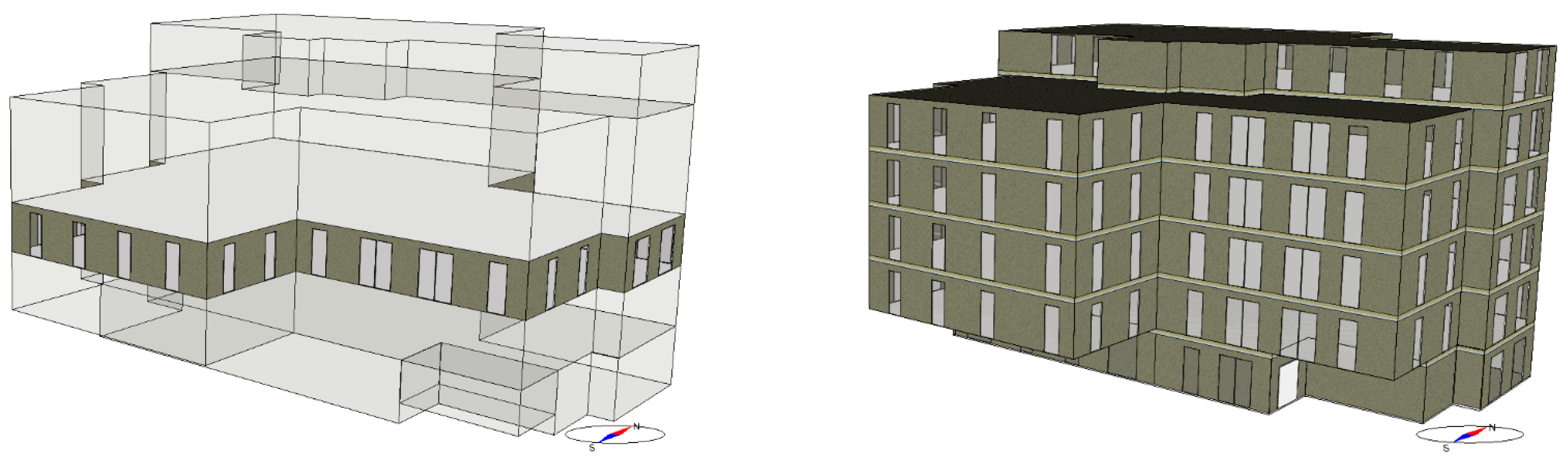
The building model was north-south oriented. The solar heat gain and transmittance coefficient of the windows were 0.35 and 0.15. Air leakage rate was 1.0 L/h at the pressure difference of 50 Pa, and thermal bridges were reported as approximately 9% of total heat losses. Besides, the building model was considered as having a standard air handling unit with 80% heat recovery facility, heating coil, cooling coil, and fans. The specific fan power was considered at 1.56 kW/(m3/s). In addition, an ideal heater and cooler with Proportional Integral (PI) control were used to keep the room temperature according to setpoints during the working hours. Also, a ventilation rate of 1.4 L/(s·m2) was found to be sufficient to keep the indoor CO2 level below 600 ppm. The views of a single floor and a whole building are shown in Figure 2. Input data for energy simulation followed the EN 16798-1:2018 standard [34,35], as shown in Table 1. When compared to analyses in [36], it can be seen that ventilation and thermal comfort input data corresponded to indoor climate Category II. In addition, metabolic rate, clothing insulation were considered of 1.2 met and 0.85 ± 0.25 clo., respectively. Considering the occupant density, the ventilation rate given in Table 1 was equivalent to 23.4 L/s per person. All input data were kept the same for all climates except the weather files. The weather file (test reference years) of Tallinn, Estonia; Brussels, Belgium; Paris, France; and Sapporo, Japan followed the American Society of Heating, Refrigerating and Air-conditioning Engineering (ASHRAE) weather files.
2.2. Continuous Variables, Cost Functions, and Cost Optimality
Two continuous variables, i.e., window transmittance and thermal resistance of wall insulation, were used. An extensive range of wall insulation thickness (0.05–0.40 m; step 0.05) and thermal transmittance of window (0.5–2.5 W/m2K; step 0.1) were studied for all climates. The range became concise based on the data cloud. The boundary condition of input data of parametric simulation is shown in Table 2. The parametric simulations were performed for a single floor model (mid-floor of the building) and a whole building model to show the effects on a different scale.
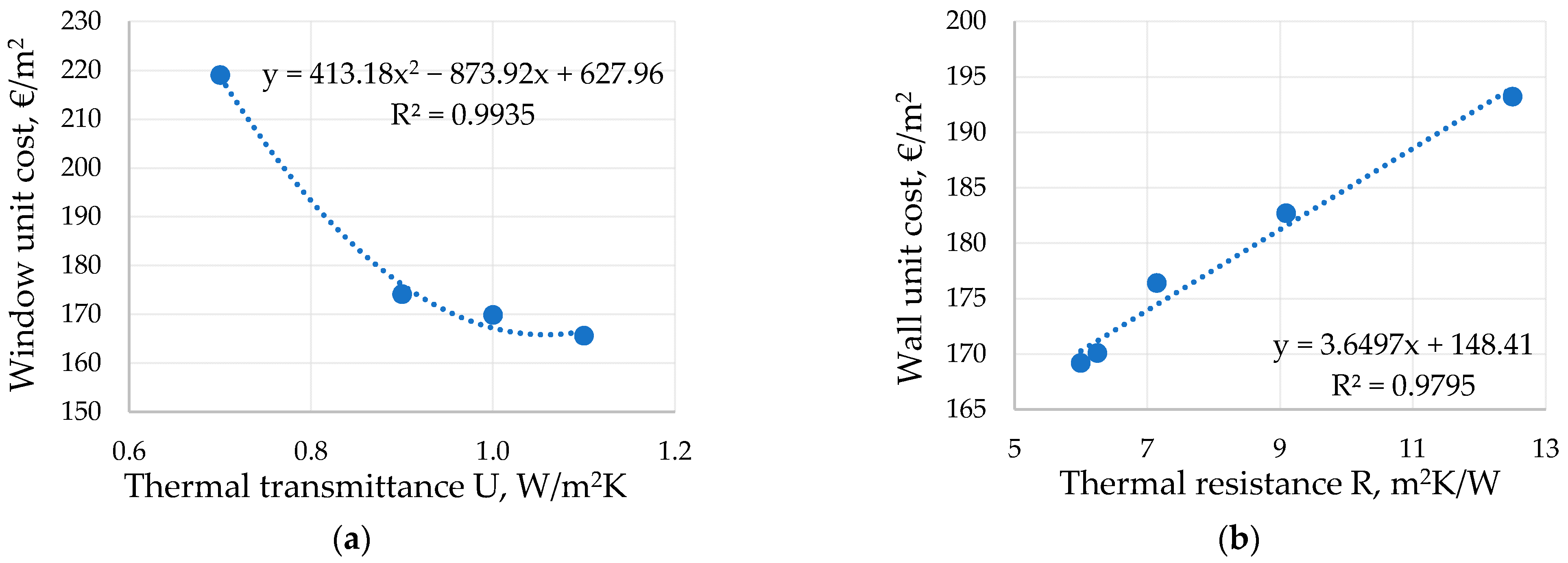
The Estonian cost functions of the window and wall insulation were used [33]. The investment cost of the window was reported as corresponding to the thermal resistance (Equation (2)), whereas the cost function of an external wall was reported corresponding to the thermal transmittance (Equation (3)). The same cost functions were used for all climates, as shown in Figure 3. These cost functions were based on brands and products available in Estonian markets and have been previously used for Estonian cost-optimal calculations.
where, is the unit cost of a window (€/m2), is the thermal transmittance of a window (W/m2K), is the unit cost of a wall (€/m2), and is the thermal resistance of a wall (m2K/W).
The cost-optimal equation was developed based on the investment cost of a wall, window, ground floor, roof, and the delivered energy cost, as shown in Equations (4)–(6). The unit cost of heating and electricity was assumed of 0.07 and 0.1 kWh/m2a, respectively. Besides, the real interest and escalation rates were assumed of 2% and 1%, respectively, for 20 years.
where, presents the value factor (−), is the real interest rate (%), is the escalation (%), is the number of years, is the total energy price considering a present value factor (€), is the heating energy use (kWh), is the heating energy price (€/kWh), is the cooling energy use (), is the cooling energy price (€/kWh), is the lowest cost (investment and operational cost) (€), is the cost of total external walls (€), is the cost of total windows (€), is the cost of a roof (€), and is the cost of a ground floor (€).
The heat transmission coefficient of the roof and ground floor were assumed discrete variables, and unit cost followed the same as the external wall. The optimal cost was found (Equation (6)), and corresponding window transmittance (U-value), the thermal resistance of wall insulation (R-value), energy need, and conductance were tabulated.
2.3. Sensitivity Analysis
This method also tested the cases of three WWR ratios (30%, 40%, and 50%), two window’s g values (0.22 and 0.35), different unit costs of heating (0.07, 0.08, and 0.10 €/kWh), and electricity (0.1, 0.12, and 0.14 €/kWh). Six combinations of WWRs and ‘g’ values were considered, as shown in Table 3. All these conducted tasks generated an acceptable range of power ‘n’.
3. Results
3.1. Degree Days and Climate Normalization Equation
Actual degree days were calculated from simulated heating energy need, Equation (7). Thus, the information about the base temperature was not needed. Area-weighted average U-value was calculated to describe the building envelope with one average U-value. This combined thermal transmittance coefficient was used to compare the climate normalized U-value (calculated from the reference Estonian cost-optimal value) to the actual cost-optimal value of the corresponding climate. Tallinn climate (Tallinn TRY weather file) was used as reference climate. However, the reference climate could be anyone out of studied climates. Based on the cost-optimal results of four climates, the degree-day ratios were calculated with Equation (8), and the power value of ‘n’ giving the best possible accuracy was estimated by Equation (9).
where, is the heating or cooling degree days (°Cd), is the energy need (kWh/m2a), is the thermal conductance of a respective building (W/K), is the heating degree days of building for a respective climate (°Cd), si the heating degree days of building for a reference (Tallinn) climate (°Cd), is the energy need for space heating in a respective climate (kWh/m2a), is the energy need for space heating in a reference climate (kWh/m2a), is the thermal conductance of building for a respective climate (W/K), is the thermal conductance of building for a reference climate (W/K), is the area weighted average thermal transmittance of building for a reference climate (W/m2K), and is the area weighted average thermal transmittance of building for a respective climate (W/m2K). The n = 0.2 value was based on the results of this study.
Note that if the building was moved from one climate to another, the cost-optimal solutions also changed. Thus, cost-optimal area-weighted U-value, conductance, and energy needs were different in all climates.
3.2. Base Temperature for Heating and Cooling
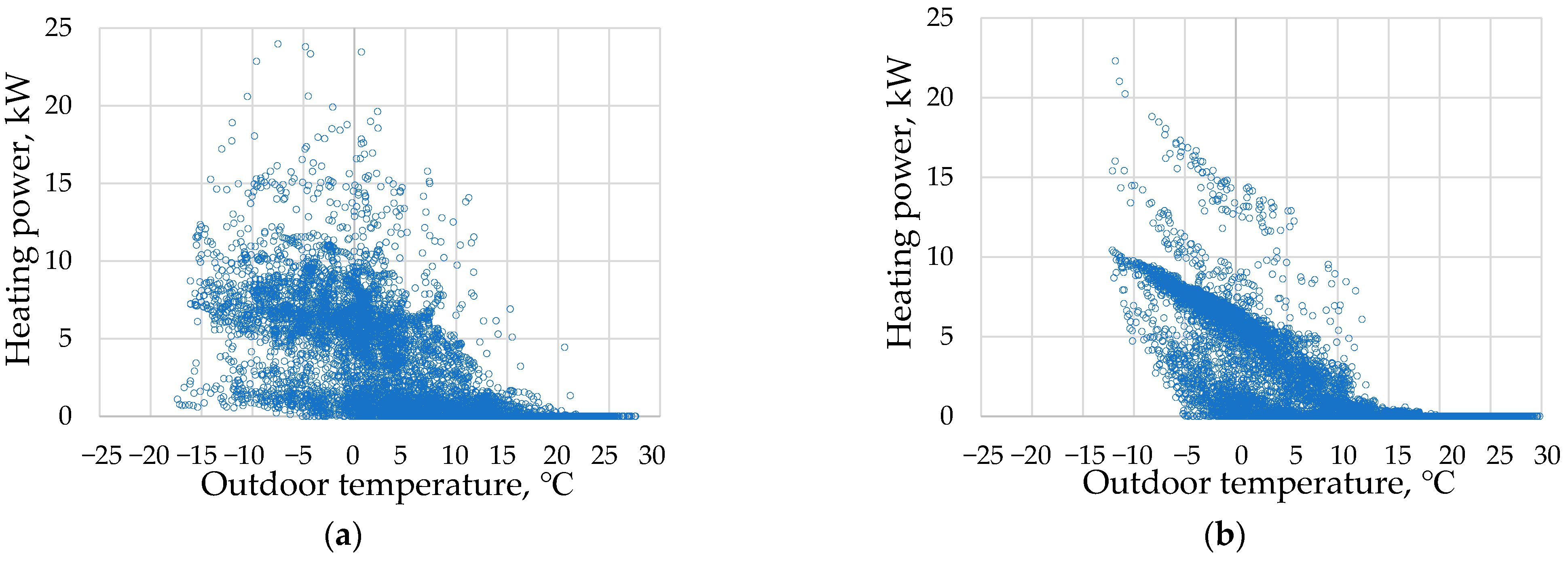
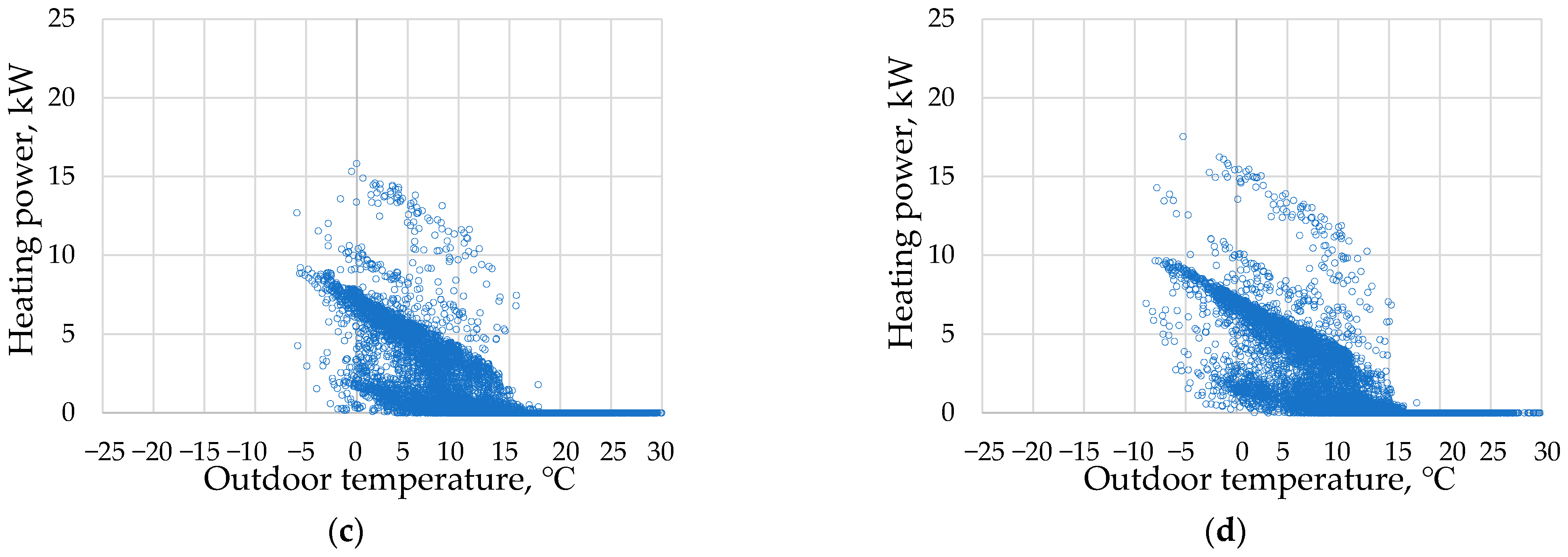
The base temperature is the cornerstone parameter if the degree days energy calculation is used. Base temperature indicates the corresponding temperature at which the building requires heating and cooling. The base temperature may be considered as a fixed value or monthly value in energy calculation methods of degree day, but in reality, it fluctuates, as can be seen from dynamic simulation results in Figure 4 and Figure 5. For instance, the base temperature in the Tallinn case varied from about −5 °C to +20 °C, which illustrates that base temperature values do not exist in modern highly energy-efficient buildings. In this study, actual degree days were calculated from simulated heating energy need with Equation (7). Average base temperature value can be calculated from the climate file by trial so that the same degree day value would be obtained, but this information was not needed in the analyses.
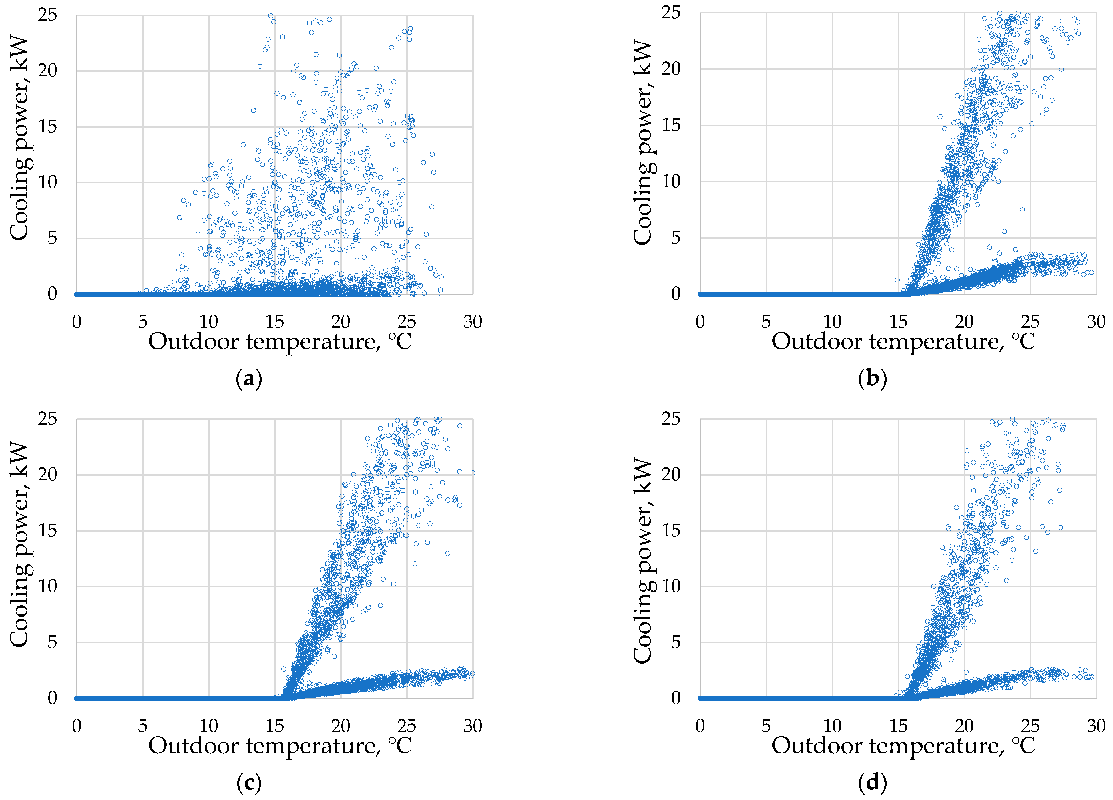
The base temperature for cooling was more established in all climates except for Tallinn’s climate, as shown in Figure 5. The scattered values for Tallinn were likely due to a low solar angle, which allowed more sunlight into the building. The ventilation system was running during 17:00–18:00 with full power, although internal heat gains from the occupants, lighting, and appliances were present until 17:00. Also, solar heat significantly increased the internal gains during 17:00–18:00, which formed the second, lower tails in the following figures.
3.3. Cost Optimal Solution Based on Investment and Heating Energy Cost
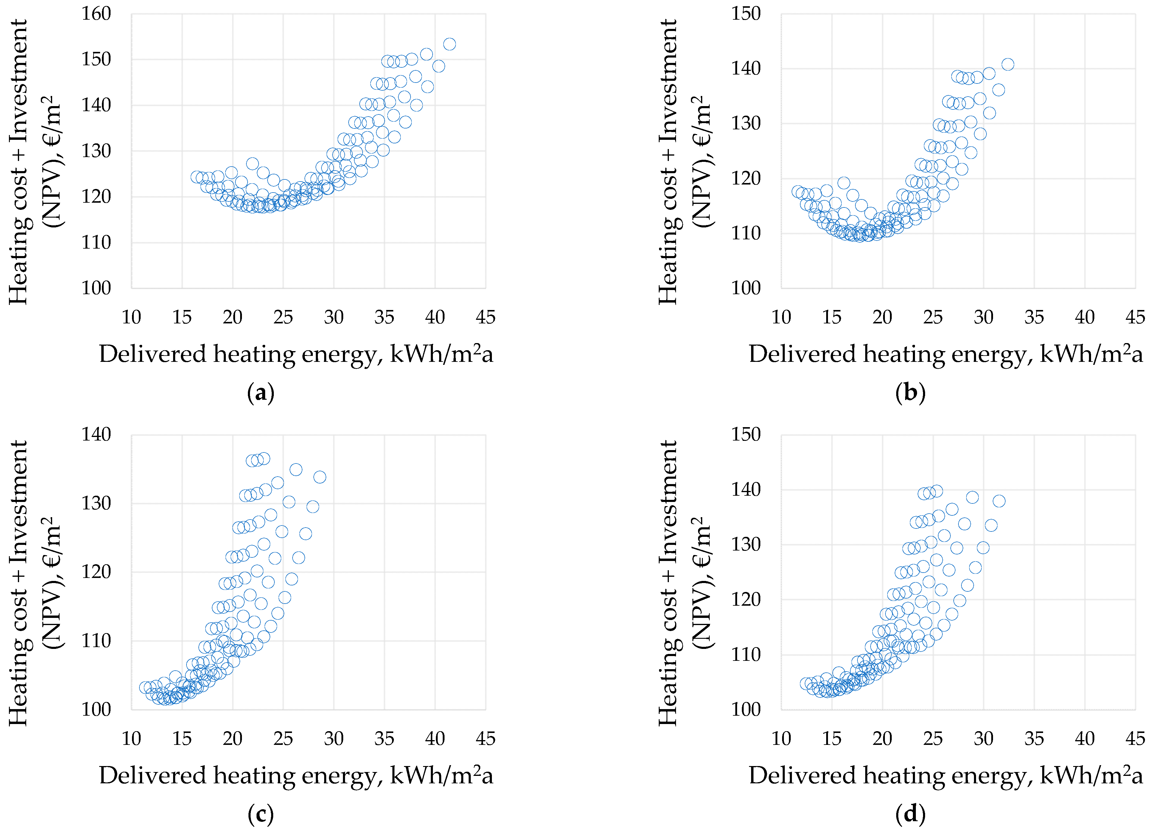
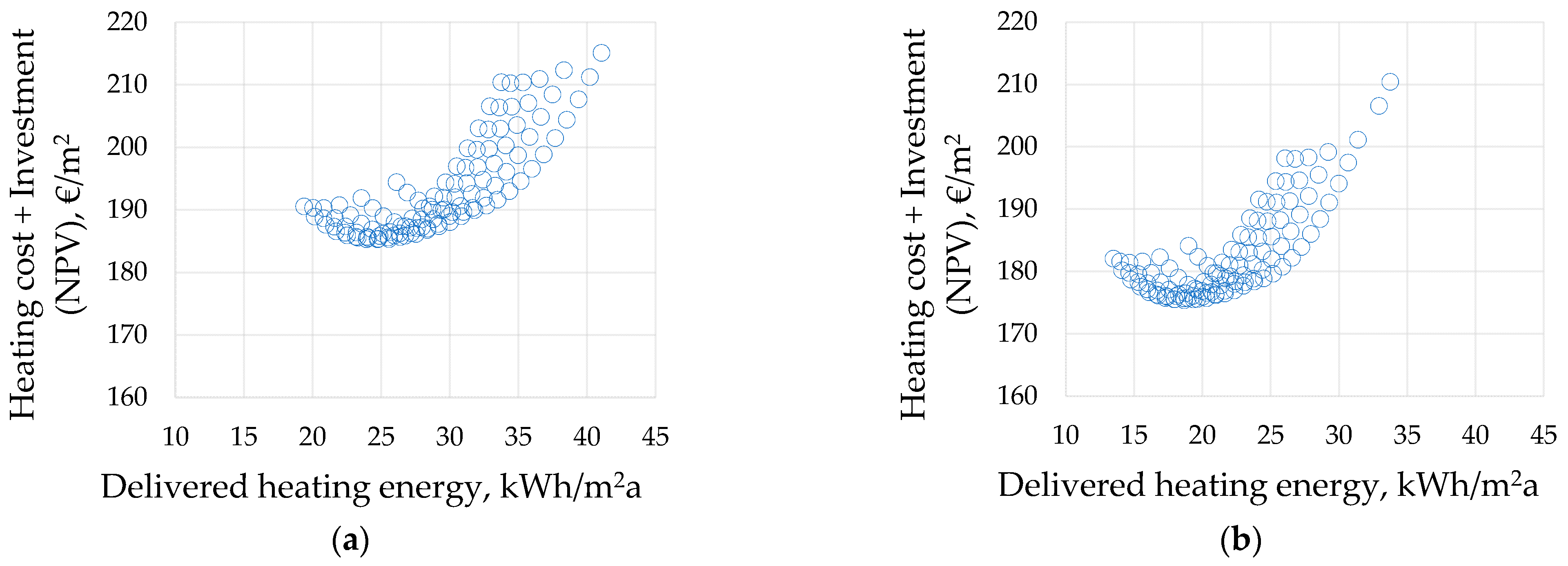
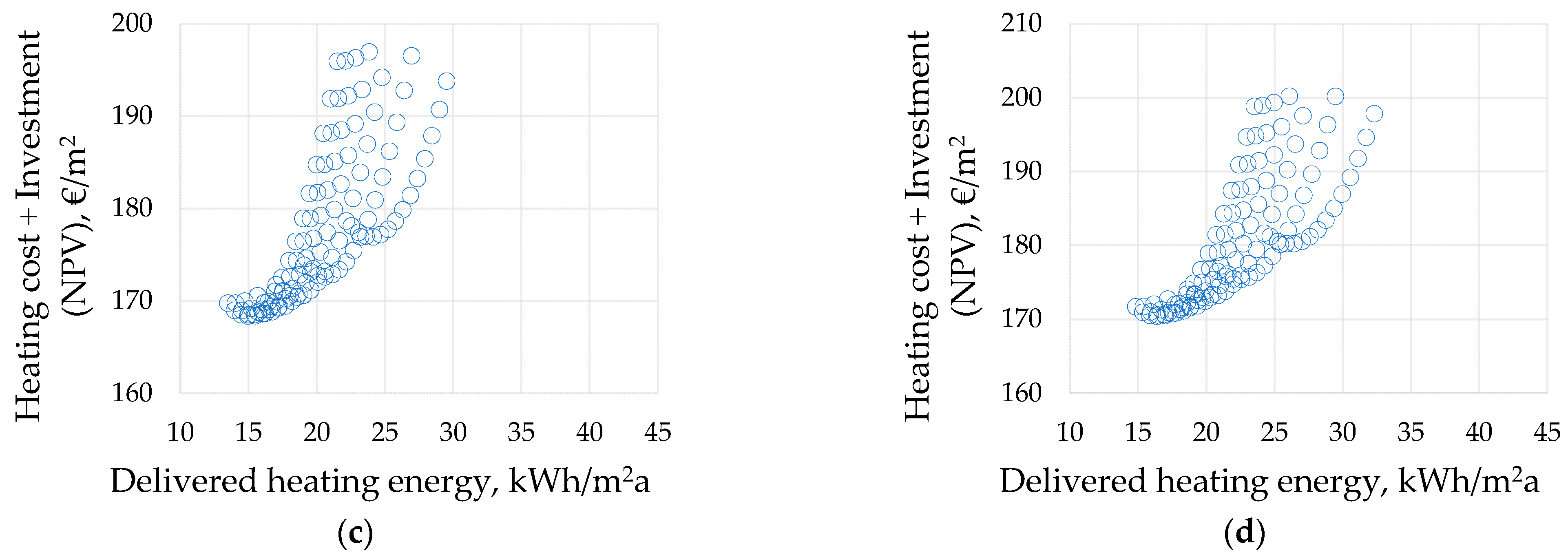
The cost-optimal solutions based on investment and heating energy costs were reported for all climates. In all cases, it was possible to find a combination of U-values of external wall and window that resulted in the smallest cost, i.e., corresponding to the cost-optimal solutions. The cost-optimal solutions for a single floor model and a whole building model are shown in Figure 6 and Figure 7, respectively. The investment cost of walls and insulation followed the function, as shown in Figure 3, and the unit costs of heating energy were 0.07 €/kWh. A WWR * g of 0.105 was used, which corresponded to 30% of WWR and a ‘g’ value of 0.35.
The objective of this study was to analyze how economic insulation thickness depends on the climate. According to the selected climates, heating needs were dominating compared to cooling needs. Because the insulation thickness affects the heating need of a building directly, the cost-optimal values were calculated only for operational heating cost and investment cost for every climate.
A good number of solutions were available; however, a single cost-optimal value was selected for every case, which had the lowest minimum cost (investment plus operational heating cost). Then, the conductance of the building envelope was calculated from the building model and was used to calculate the degree days with Equation (7).
The cost-optimal solutions for a single floor model and a whole building model based on heating energy needs are shown in Table 4. The heating degree days and building envelope conductance were calculated with Equations (7) and (8). Area weighted thermal transmittance of the building envelope was compared to the normalized value that was calculated with Equation (9) from Tallinn reference values. Two normalized thermal transmittance values, one calculated with power n = 0.5 (square root) and another calculated with n = 0.2 were reported. The smaller the difference between average U-value and normalized U-value, the better the accuracy of the climate normalization (Equation (9)). The climate normalized U-values were close to actual values with power n = 0.2 both in the case of the single floor and whole building models, as shown in Figure 8.
The effects of the model size (single floor vs. whole building) were quite small on cost-optimal external wall and window U-values as well as on normalized area-weighted average U-value. The method also demonstrates that it is possible to avoid the use of the base temperature, which is typical for degree days methods. In the following, the proposed method will be tested with parametric analyses for different scenarios, which would have effects on the cost-optimal values.
3.4. Sensitivity Analysis Based on Investment and Heating Energy Cost
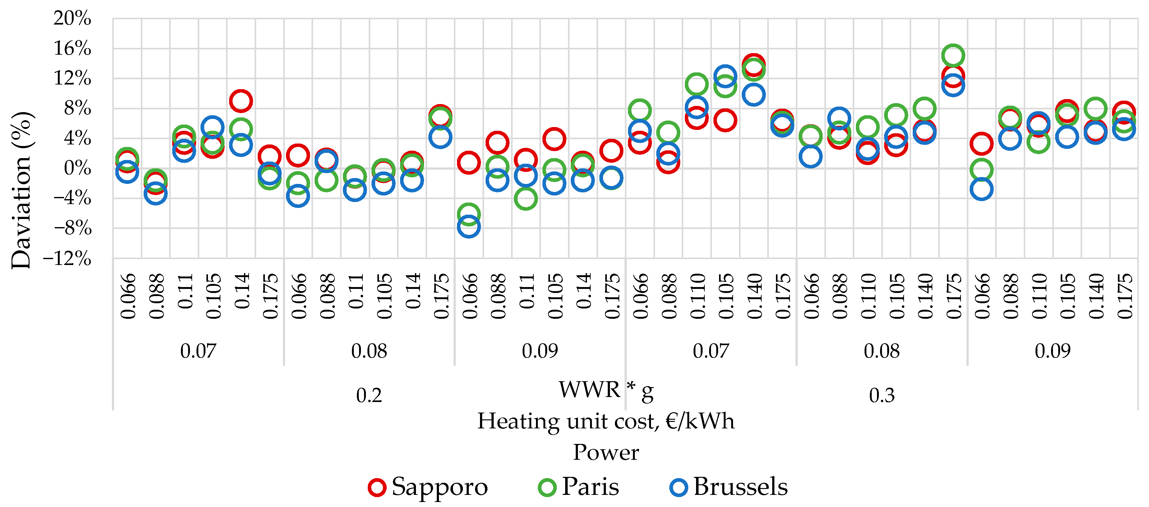
The normalization accuracy can be affected by different window sizes, g-values, and cost data, which are shown in Figure 9. Results obtained with a power value of 0.2 showed lower deviations compared to the power value of 0.3. However, the heating unit cost did not show any visible correlation due to changing the cost-optimal solution. The overall deviations remained between −8% and 15%. Furthermore, 0%–0.2% of total occupant hours were found beyond the limit of 21–25.5 °C, which was far less than 3%.
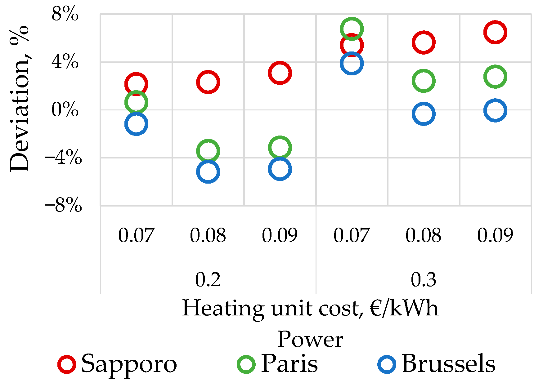
Similar sensitivity analysis was conducted for a whole building model, which results are shown for a case of WWR * g = 0.105 (30% WWR and g value of 0.35) in Figure 10. The results showed the overall deviations were between −5% and 7%.
The effects of ‘n’ value from 0.15–0.30 with a step of 0.05 are illustrated in Figure 11. In the case of a single floor model, the range of 0.15 to 0.25 gave the smallest deviations, but generally, the optimal value depends on the climate and heating energy price. For the whole building model, the slightly higher values of 0.25 and 0.30, gave the best accuracy.
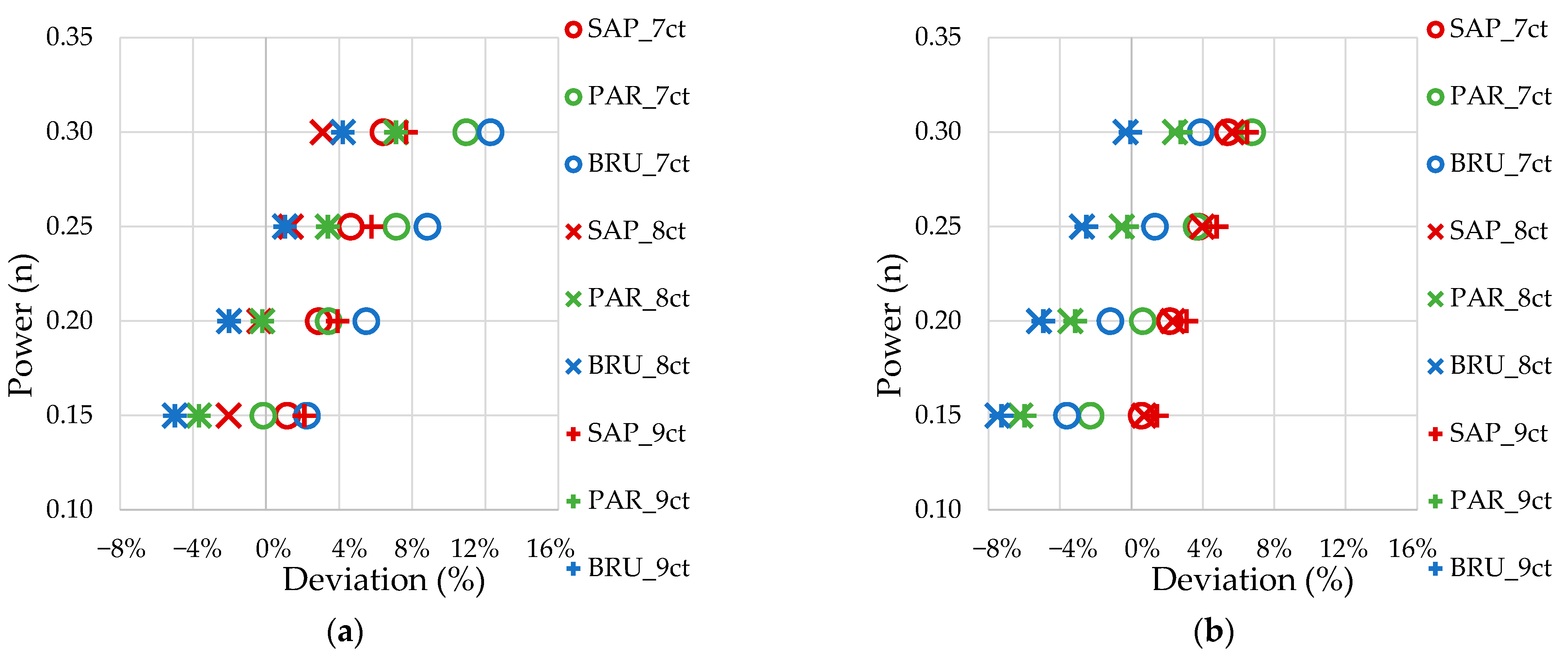
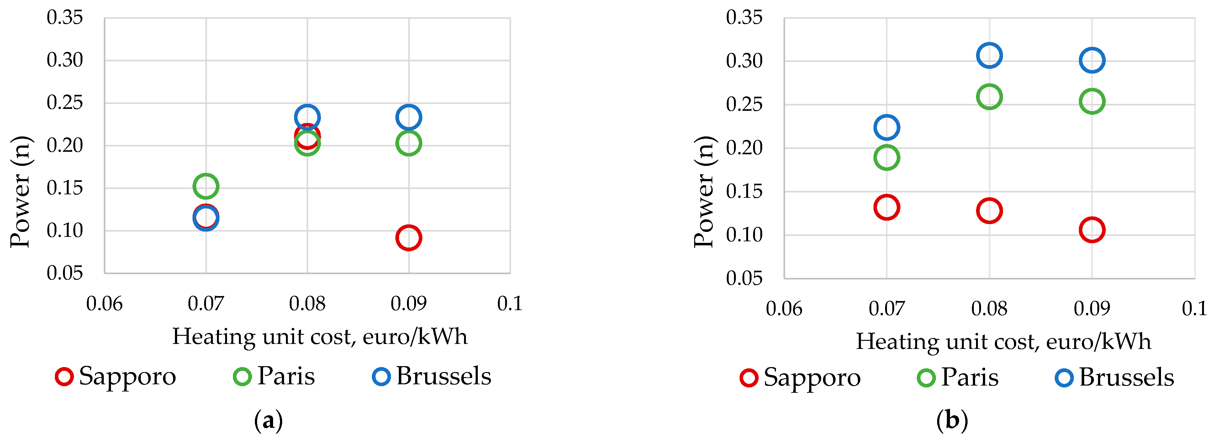
The power values of ‘n’ at which there was no deviation between actual and normalized ‘U-value’ are shown in Figure 12 for the WWR * g = 0.105 case (30% WWR and g value of 0.35). The overall range of power values was 0.09–0.31, and the range was especially narrow for the single floor model at heating energy costs of 0.07 and 0.08 €/kWh.
3.5. Cost Optimal Solution based on Investment and Total Energy Cost
In the following, the cooling energy was also accounted for, in addition to heating energy, in order to find the cost-optimal solutions based on investment and total energy cost (both heating and cooling energy cost) for all climates, as shown in Table 5. The detailed process follows the one discussed in Section 3.3.
The results showed that the proposed method normalized the U-values to different climates with poor accuracy when the cooling was included, as maximum deviations varied from −8.0% to −5.6%. The accuracy of the whole building model was much worse compared to heating energy, where the maximum deviation of 2%, as shown in Table 4. This indicates that U-values have no significant effect on cooling energy, which depends on other factors.
3.6. Sensitivity Analysis Based on Investment and Total Energy Cost
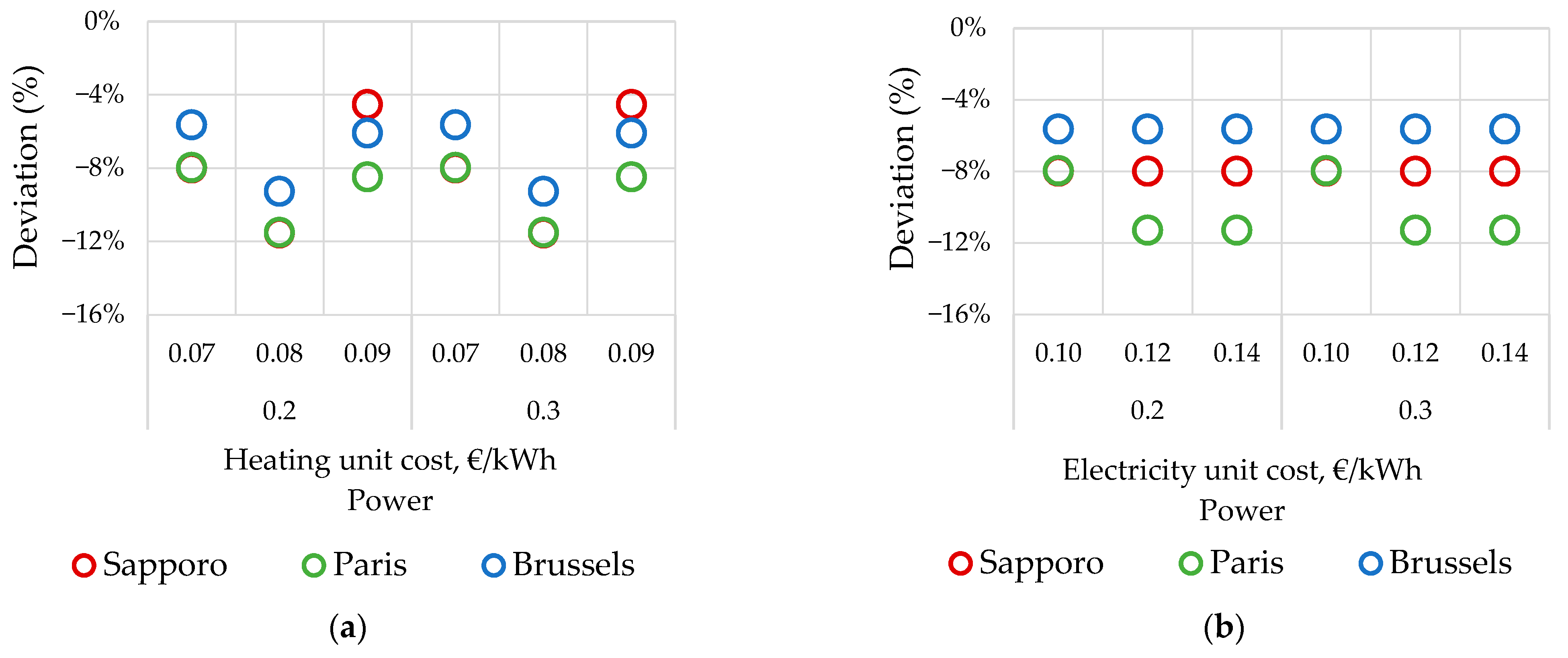
The proposed method was tested with a whole building model. The results are presented for a case of 0.105 (Table 3) where the WWR and ‘g’ value of windows were 30% and 0.35, respectively. The effects of the unit cost of energy and power value of ‘n’ on the deviation of normalized heat transmission are illustrated in Figure 13. The horizontal axis shows two parameters, namely the unit cost of energy and power ‘n’ (Equation (9)), whereas the vertical axis shows the deviations corresponding to the different combinations.
The investment cost varied up to 2.5% among different climates due to using the same cost function for all climates. Besides, the cost of used energy was varied up to 37% compared to the reference Tallinn climate. The reference Tallinn climate had harsh winter conditions compared to Paris and Brussels, which increased the heating energy needs. Thus, the unit cost of heating was more dominating compared to the unit cost of electricity due to the high heating demand and low electricity demand, as shown in Figure 13. The overall deviations were between −11.5% and −4.5% (Figure 13a) and −11.3% and −5.6% (Figure 13b). Furthermore, the same building envelope insulation solution could not ensure the same energy-saving potential for different climates.
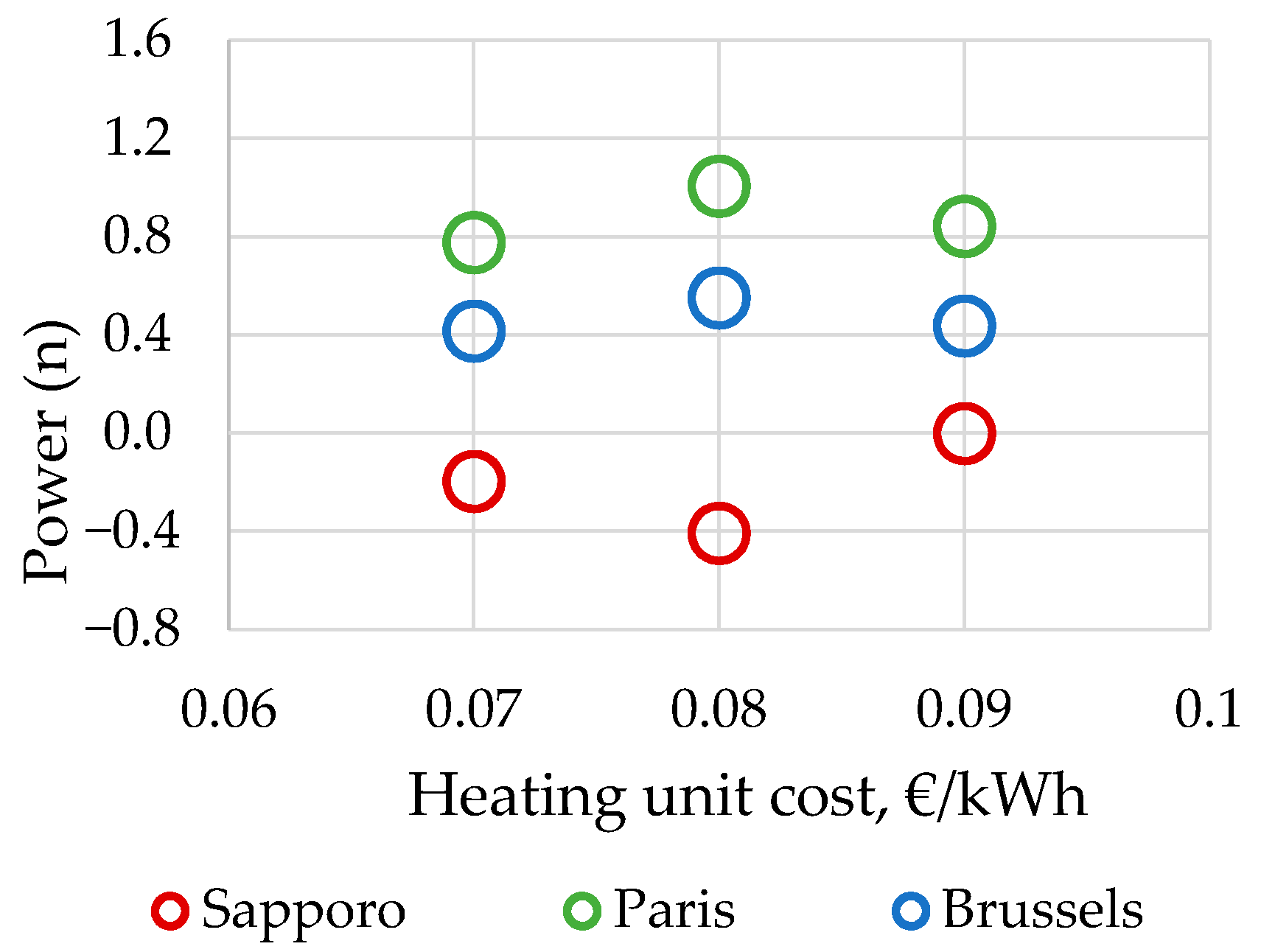
Additionally, the power values were determined at which there were no deviations, i.e., provide accurate climate normalization, Figure 14. The results are shown for WWR * g = 0.105 (product of 30% WWR and g value of 0.35) and a fixed unit cost of electricity (0.1 €/kWh). Sapporo climate showed zero deviations at negative power values due to the high combined energy need compared to the Tallinn case. Moreover, the heating need for Paris and Brussels cases were less compared to the Tallinn case, but opposite observations were found for the cooling need. Though the cooling needs were high, the overall effect on the cost-optimal solution was less meaningful due to the high energy efficiency ratio (EER) of the cooling system (EER = 3.5). Therefore, the results of Figure 14 show that the method is not applicable and should not be used for cooling normalization.
3.7. Application of the Method on a Monthly Basis
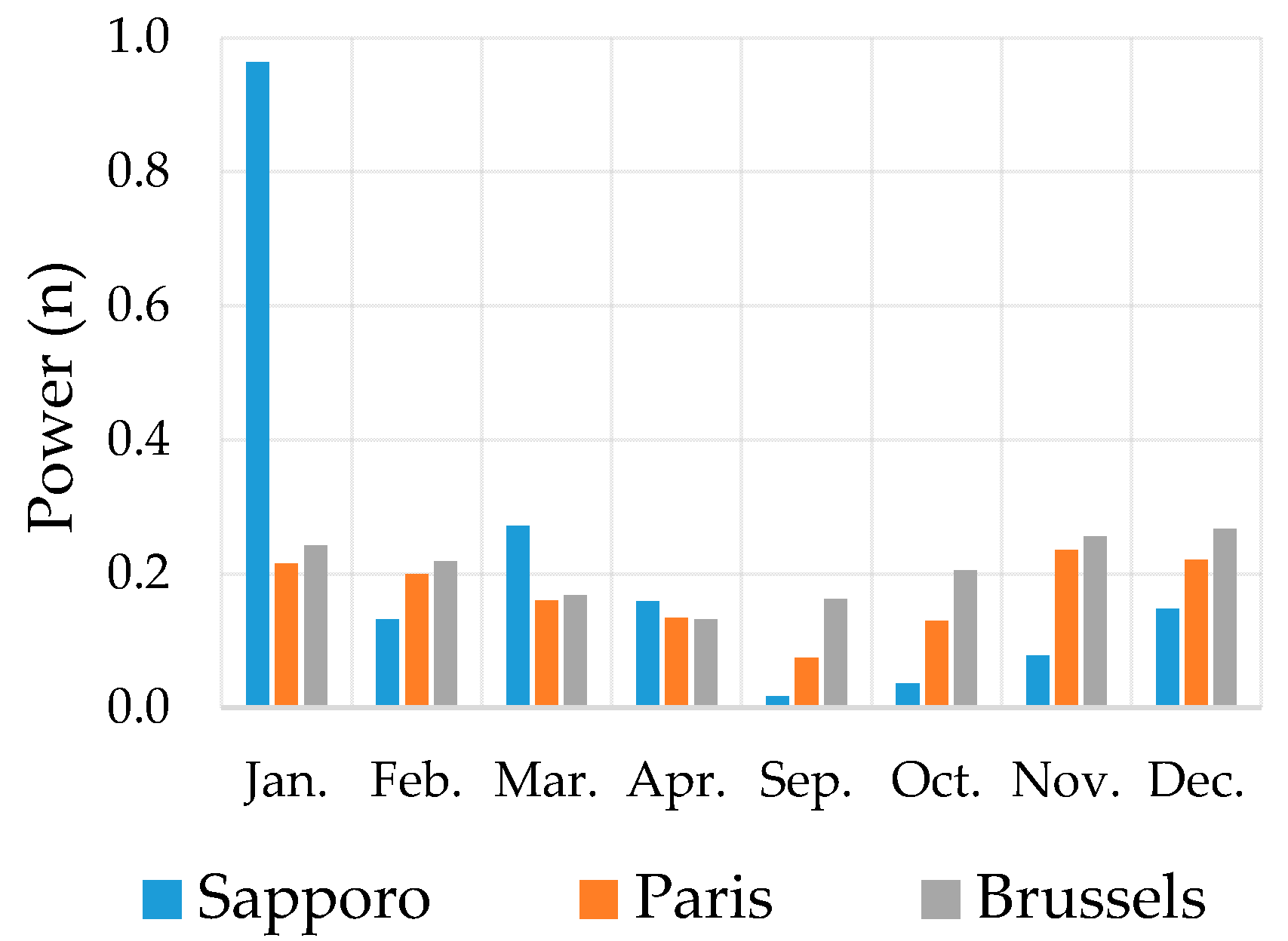
Previous analyses showed that the optimal insulation normalization determined from the heating energy cost-optimal solution worked well on an annual basis. A similar calculation to Section 3.4 was repeated on a monthly basis to show which accuracy the normalization can be applied for the monthly heating energy. Monthly power values calculated from monthly actual degree days are shown in Figure 15.
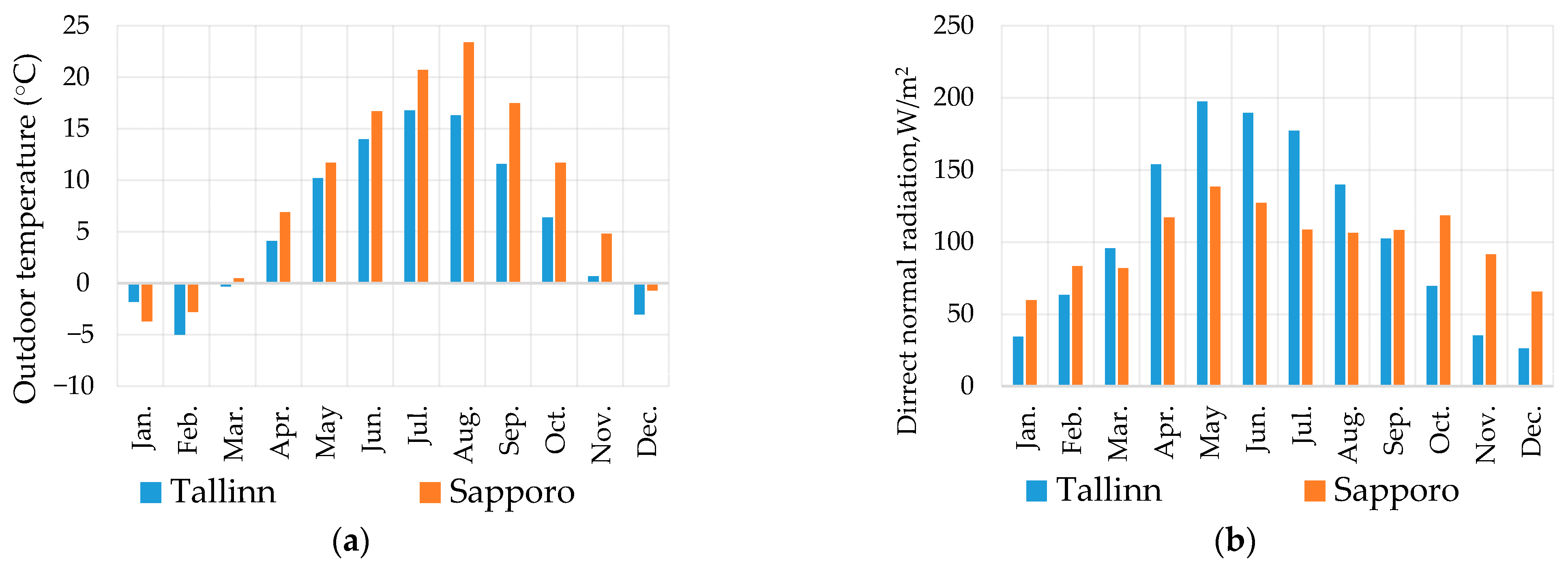
The monthly normalization worked reasonably well (the power factor close to 0.2) when monthly climate differences were reasonably similar to the annual climate differences. For Sapporo, this was not the case for January, whereas other months showed consistent results. In the Sapporo case, a power factor of 0.96 for January was explained by colder outdoor temperatures in January, while the annual outdoor temperature value was lower for Tallinn. For all other months, the outdoor temperature was higher in Sapporo, as shown in Figure 16.
4. Conclusions
This study developed a new equation for the assessment of building envelopes’ optimal insulation in different climates for office buildings. The developed method suggests determining actual degree days from simulated heating energy need and the thermal conductance of a building, avoiding in such a way the use of the base temperature. The method was tested in four climates and validated against cost-optimal solutions solved with optimization. The accuracy of the method was assessed with sensitivity analyses of key parameters such as WWRs, window g-values, costs of heating, and electricity.
For the validation of the developed method, the cost-optimal solutions for every climate based on cost functions of external wall and windows as well as energy costs were determined, resulting in area-weighted average U-values in all four climates. The actual degree days were calculated for every climate with Equation (7). These results allowed testing of the performance of the existing square root formula (Equation (1)), showing that the climate difference effect was overestimated, i.e., calculation from the cold climate U-value would result in less insulation than cost-optimal in warmer climates. Parametric analyses revealed that the power value would provide the best possible accuracy and varied between n = 0.15 and 0.30, but n = 0.2 worked well in all cases and can be recommended as a default value.
An attempt was made to apply an optimal insulation method with heating and cooling energy in order to describe also climate differences effect on cooling energy. However, as the insulation thickness and U-value of the window have a direct effect on the heating energy but minimal effect on cooling energy, the normalization based on the total energy (heating and cooling) was not successful. Therefore, the cooling energy differences caused by climate cannot be described by insulation.
In the cost optimization, indoor air quality was not compromised because Category II ventilation rates were used in all cases. The use of the room air temperature setpoint means that operative temperature and thermal comfort can be changed when the external wall and window U-values are varied. However, the cost-optimal U-values reported in Table 4 show high thermal insulation level, and simulated operative temperatures fall well to Category II range with used 21 °C heating setpoint. Around 99.8% of indoor temperature were in the range of 21–25.5 °C.
Sensitivity analyses with a broad range of energy costs, WWR, and g-values of windows revealed that the developed equation resulted in maximum 5% underestimation and maximum 7% overestimation of an average area-weighted optimal U-value of building envelope in another climate. While the method is expected to be applied mostly for insulation or annual heating energy comparisons, the actual degree days were also calculated on a monthly basis and also showed consistent performance on a monthly level.
The developed method allows objectively to compare optimal insulation of the building envelope in different climates. The method is easy to apply for energy performance comparison of similar buildings in different climates and also for energy performance requirements comparison.
Author Contributions
K.A. wrote the paper and conceived, designed, and performed the simulations. J.K. was the principal investigator responsible for the study design. All authors have read and agreed to the published version of the manuscript.
Funding
This research received no external funding.
Institutional Review Board Statement
“Not applicable” for studies not involving humans or animals.
Informed Consent Statement
“Not applicable” for studies not involving humans.
Data Availability Statement
Not applicable.
Acknowledgments
This research was supported by the K.V. Lindholms Stiftelse foundation, by the Estonian Centre of Excellence in Zero Energy and the Resource Efficient Smart Buildings and Districts, ZEBE, grant 2014-2020.4.01.15-0016 funded by the European Regional Development Fund and by the European Commission through the H2020 project Finest Twins (grant No. 856602).
Conflicts of Interest
The authors declare no conflict of interest.
Abbreviation
| Cooling energy price, €/kWh | |
| Total energy price with considering the present value factor, € | |
| The lowest cost (investment and operational cost), € | |
| Cost of a ground floor, € | |
| Cost of a roof, € | |
| Cost of a total external wall, € | |
| Cost of total windows, € | |
| Heating or cooling degree days, °Cd | |
| Escalation, % | |
| Energy need, kWh/m2a | |
| Cooling energy use, kWh | |
| Heating energy use, kWh | |
| Energy need for space heating in a respective climate, kWh/m2a | |
| Energy need for space heating in a reference climate, kWh/m2a | |
| EER | Energy efficiency ratio, - |
| Present value factor, - | |
| Thermal conductance of a respective building, W/K | |
| Thermal conductance of building for a respective climate, W/K | |
| Thermal conductance of building for a reference climate, W/K | |
| Heating energy price, €/kWh | |
| Heating degree days of building for a respective climate, °Cd | |
| Heating degree days of building for a reference climate, °Cd | |
| Number of years, year | |
| Real interest rate, % | |
| Area weighted average thermal transmittance for a reference climate, W/m2K | |
| Optimal thermal transmittance of respective building for a reference climate, W/m2K | |
| Area weighted average thermal transmittance for a respective climate, W/m2K | |
| Optimal thermal transmittance of building for a respective climate, W/m2K | |
| Thermal transmittance of a window, W/m2K | |
| Thermal resistance of a wall, m2K/W | |
| Unit cost of a window, €/m2 | |
| Unit cost of a wall, €/m2 |
References
- Building Performance Institute Europe (BPIE). Europe’s Building under the Microscope. A Country-by-Country Review of the Energy Performance of Buildings; Buildings Performance Institute Europe BPIE: Brussels, Belgium, 2011. [Google Scholar]
- EURAC. D2.1a—Survey on the Energy Needs and Architectural Features of the EU Building Stock iNSPiRE Project—Development of Systemic Packages for Deep Energy Enovation of Residential and Tertiary Buildings including Envelope and Systems; BSRIA: Bracknell, UK, 2014; pp. 33–46. [Google Scholar]
- Commission Recommendation (EU). 2016/1318 of 29 July 2016 on Guidelines for the Promotion of Nearly Zero-Energy Buildings and Best Practices to Ensure That, by 2020, All New Buildings Are Nearly Zero-Energy Buildings; Commission Recommendation (EU), European Commission: Brussels, Belgium, 2016. [Google Scholar]
- Eisenhower, B.; O’Neill, Z.; Fonoberov, V.A.; Mezić, I. Uncertainty and sensitivity decomposition of building energy models. J. Build. Perform. Simul. 2012, 5, 171–184. [Google Scholar] [CrossRef]
- Bucking, S.; Zmeureanu, R.; Athienitis, A. A methodology for identifying the influence of design variations on building energy performanc. J. Build. Perform. Simul. 2014, 7, 411–426. [Google Scholar] [CrossRef]
- Sun, Y.; Heo, Y.; Tan, M.; Xie, H.; Wu, C.F.J.; Augenbroe, G. Uncertainty quantification of microclimate variables in building energy models. J. Build. Perform. Simul. 2014, 7, 17–32. [Google Scholar] [CrossRef]
- Kaynakli, O. A review of the economical and optimum thermal insulation thickness for building applications. Renew. Sustain. Energy Rev. 2012, 16, 415–425. [Google Scholar] [CrossRef]
- European Commission. Commission Delegated Regulation (EU) No 244/2012 of 16 January 2012 supplementing Directive 2010/31/EU of the European Parliament and of the Council on the Energy Performance of Buildings by Establishing a Comparative Methodology Framework for Calculating Cost-Optimal Levels of Minimum Energy; European Commission: Brussels, Belgium, 2012. [Google Scholar]
- Ibrahim, M.; Ghaddar, N.; Ghali, K. Optimal location and thickness of insulation layers for minimizing building energy consumption. J. Build. Perform. Simul. 2012, 5, 384–398. [Google Scholar] [CrossRef]
- Rosti, B.; Omidvar, A.; Monghasemi, N. Optimal insulation thickness of common classic and modern exterior walls in different climate zones of Iran. J. Build. Eng. 2020, 27, 100954. [Google Scholar] [CrossRef]
- Bolattürk, A. Determination of optimum insulation thickness for building walls with respect to various fuels and climate zones in Turkey. Appl. Therm. Eng. 2006, 26, 1301–1309. [Google Scholar] [CrossRef]
- D’Agostino, D.; Rossi, F.d.; Marigliano, M.; Marino, C.; Minichiello, F. Evaluation of the optimal thermal insulation thickness for an office building in different climates by means of the basic and modified “cost-optimal” methodology. J. Build. Eng. 2019, 24, 100743. [Google Scholar] [CrossRef]
- Ucar, A.; Balo, F. Determination of the energy savings and the optimum insulation thickness in the four different insulated exterior walls. Renew. Energy 2010, 35, 88–94. [Google Scholar] [CrossRef]
- Ozel, M. Determination of optimum insulation thickness based on cooling transmission load for building walls in a hot climate. Energy Convers. Manag. 2013, 66, 106–114. [Google Scholar] [CrossRef]
- Dylewski, R.; Adamczyk, J. Economic and environmental benefits of thermal insulation of building external walls. Build. Environ. 2011, 46, 2615–2623. [Google Scholar] [CrossRef]
- Jaber, S.; Ajib, S. Thermal and economic windows design for different climate zones. Energy Build. 2011, 43, 3208–3215. [Google Scholar] [CrossRef]
- Kontoleon, K.J.; Zenginis, D.G. Analysing Heat Flows Through Building Zones in Aspect of their Orientation and Glazing Proportion, under Varying Conditions. Procedia Environ. Sci. 2017, 38, 348–355. [Google Scholar] [CrossRef]
- Thalfeldt, M.; Ergo, P.; Kurnitski, J.; Hendrik, V. Facade design principles for nearly zero energy buildings in a cold climate. Energy Build. 2013, 67, 309–321. [Google Scholar] [CrossRef]
- Pikas, E.; Thalfeldt, M.; Kurnitski, J. Cost optimal and nearly zero energy building solutions for office buildings. Energy Build. 2014, 74, 30–42. [Google Scholar] [CrossRef]
- Yu, J.; Yang, C.; Tian, L.; Liao, D. A study on optimum insulation thicknesses of external walls in hot summer and cold winter zone of China. Appl. Energy 2009, 86, 2520–2529. [Google Scholar] [CrossRef]
- Karlsson, J.; Roos, A.; Karlsson, B. Building and climate influence on the balance temperature of buildings. Build. Environ. 2003, 38, 75–81. [Google Scholar] [CrossRef]
- Harvey, L.D.D. Using modified multiple heating-degree-day (HDD) and cooling-degree-day (CDD) indices to estimate building heating and cooling loads. Energy Build. 2020, 229, 110475. [Google Scholar] [CrossRef]
- Calise, F.; D’Accadia, D.M.; Barletta, C.; Battaglia, V.; Pfeifer, A.; Duic, N. Detailed modelling of the deep decarbonisation scenarios with demand response technologies in the heating and cooling sector: A case study for Italy. Energies 2017, 10, 1535. [Google Scholar] [CrossRef]
- Granja, A.D.; Labaki, L.C. Influence of External Surface Colour on the Periodic Heat Flow through a Flat Solid Roof with Variable Thermal Resistance; John Wiley Sons Ltd: Hoboken, NJ, USA, 2003; pp. 771–779. [Google Scholar]
- Daouas, N.; Hassen, Z.; Aissia, H.B. Analytical periodic solution for the study of thermal performance and optimum insulation thickness of building walls in Tunisia. Appl. Therm. Eng. 2010, 30, 319–326. [Google Scholar] [CrossRef]
- Ahmed, K.; Carlier, M.; Feldmann, C.; Kurnitski, J. A new method for contrasting energy performance and near-zero energy building requirements in different climates and countries. Energies 2018, 11, 1334. [Google Scholar] [CrossRef] [Green Version]
- Ahmed, K.; Yoon, G.; Ukai, M.; Kurnitski, J. How to compare energy performance requirements of Japanese and European office buildings. In Proceedings of the E3S Web of Conference 111, Clima, Bucharest, Romania, 26–29 May 2019. [Google Scholar]
- Seppänen, O. Rakennusten Lämmitys, 2nd ed.; Gummerus Oy: Jyväskylä, Finnish, 2001. [Google Scholar]
- IDA Indoor Climate and Energy, Equa Simulations AB. Available online: http://www.equa.se/en/ida-ice/ (accessed on 24 December 2015).
- Sahlin, P. Modeling and Simulation Methods for Modular Continuous System in Buildings; Doctoral Dissertation KTH: Stockholm, Sweden, 1996. [Google Scholar]
- EN ISO 13791. Thermal Performance of Buildings. Calculation of Internal of a Room in Summer without Mecahanical Cooling. General Criteria and Validation Procedures; CEN European Committee for Standardization: Brussels, Belgium, 2004.
- Travesi, J.; Maxwell, G.; Klaassen, C.; Holtz, M. Empirical Validation of IOWA Energy Resource Station Building Energy Analysis Simulation Models, Report of Task 22, Subtask Building Energy Analysis Tools; International Energy Agency—Solar heating and Cooling Programme: Paris, France, 2001. [Google Scholar]
- Simson, R.; Arumägi, E.; Kuusk, K.; Kurnitski, J. Redefining cost-optimal nZEB levels for new residential buildings. In Proceedings of the E3S Web of Conferences 111, 03035, CLIMA, Bucharest, Romania, 26–29 May 2019. [Google Scholar]
- Ahmed, K.; Akhondzada, A.; Kurnitski, J.; Olesen, B. Occupancy schedules for energy simulation in New prEN16798-1 and ISO/FDIS 17772-1 standards. Sustain. Cit. Soc. 2017, 35, 134–144. [Google Scholar] [CrossRef] [Green Version]
- Ahmed, K.; Kurnitski, J.; Olesen, B. Data for occupancy internal heat gain calculation in main building categories. Data Brief 2017, 15, 1030–1034. [Google Scholar] [CrossRef] [PubMed] [Green Version]
- Alfano, F.R.A.; Olesen, B.W.; Palella, I.B.; Riccio, G. Thermal comfort: Design and assessment for energy saving. Energy Build. 2014, 81, 326–336. [Google Scholar] [CrossRef]
Figure 1.
Optimum insulation thickness [7].
Figure 1.
Optimum insulation thickness [7].

Figure 2.
Views of a single floor and whole building model.

Figure 3.
According to Estonian real estate market the unit investment cost of (a) window and (b) wall.
Figure 3.
According to Estonian real estate market the unit investment cost of (a) window and (b) wall.

Figure 4.
Illustration of the non-existing base temperature of heating degree day (HDD) for different climates; the plot of hourly heating powers (a) Tallinn, (b) Sapporo, (c) Paris, and (d) Brussels.
Figure 4.
Illustration of the non-existing base temperature of heating degree day (HDD) for different climates; the plot of hourly heating powers (a) Tallinn, (b) Sapporo, (c) Paris, and (d) Brussels.


Figure 5.
Base temperature of cooling degree day (CDD) for different climates (a) Tallinn, (b) Sapporo, (c) Paris, and (d) Brussels.
Figure 5.
Base temperature of cooling degree day (CDD) for different climates (a) Tallinn, (b) Sapporo, (c) Paris, and (d) Brussels.

Figure 6.
Cost optimal solution of a single floor model based on heating energy-related cost and investment cost in different climates (a) Tallinn, (b) Sapporo, (c) Paris, and (d) Brussels.
Figure 6.
Cost optimal solution of a single floor model based on heating energy-related cost and investment cost in different climates (a) Tallinn, (b) Sapporo, (c) Paris, and (d) Brussels.

Figure 7.
Cost optimal solution of a whole building model based on heating energy-related cost and investment cost for different climates (a) Tallinn, (b) Sapporo, (c) Paris, and (d) Brussels.
Figure 7.
Cost optimal solution of a whole building model based on heating energy-related cost and investment cost for different climates (a) Tallinn, (b) Sapporo, (c) Paris, and (d) Brussels.


Figure 8.
Accuracy of the normalization calculated as the difference of average U-value vs. normalized U-value (a) single floor model, (b) whole building model.
Figure 8.
Accuracy of the normalization calculated as the difference of average U-value vs. normalized U-value (a) single floor model, (b) whole building model.

Figure 9.
Deviation of normalized U-value of a single floor model for the case of fixed electricity unit cost (lowest cost-optimal solution based on investment and operational heating cost).
Figure 9.
Deviation of normalized U-value of a single floor model for the case of fixed electricity unit cost (lowest cost-optimal solution based on investment and operational heating cost).

Figure 10.
Deviation of normalized U-value of a whole building model for the case of fixed electricity unit cost (lowest cost-optimal solution based on investment and operational heating cost).
Figure 10.
Deviation of normalized U-value of a whole building model for the case of fixed electricity unit cost (lowest cost-optimal solution based on investment and operational heating cost).

Figure 11.
Effect of power and heating unit cost on the deviation (a) single floor model, (b) whole building model (cost-optimal solution based on investment and operational heating cost).
Figure 11.
Effect of power and heating unit cost on the deviation (a) single floor model, (b) whole building model (cost-optimal solution based on investment and operational heating cost).

Figure 12.
Range of power which gives no deviation compared to reference climate for cases of (a) Heating energy of single floor model, (b) Heating energy of a whole building model.
Figure 12.
Range of power which gives no deviation compared to reference climate for cases of (a) Heating energy of single floor model, (b) Heating energy of a whole building model.

Figure 13.
Deviation of normalized average U-value for a whole building model (a) Electricity unit cost is fixed to 0.1 €/kWh, (b) Heating unit cost is fixed to 0.07 €/kWh (lowest cost-optimal solution based on investment and operational heating and cooling cost).
Figure 13.
Deviation of normalized average U-value for a whole building model (a) Electricity unit cost is fixed to 0.1 €/kWh, (b) Heating unit cost is fixed to 0.07 €/kWh (lowest cost-optimal solution based on investment and operational heating and cooling cost).

Figure 14.
Range of power, which gives no deviation compare to reference climate for cases of the total energy of the whole building model.
Figure 14.
Range of power, which gives no deviation compare to reference climate for cases of the total energy of the whole building model.

Figure 15.
Monthly power values for different climates corresponding to the reference Tallinn climate.
Figure 15.
Monthly power values for different climates corresponding to the reference Tallinn climate.

Figure 16.
The comparison of Tallinn and Sapporo climates (a) outdoor temperature and (b) direct solar radiation.
Figure 16.
The comparison of Tallinn and Sapporo climates (a) outdoor temperature and (b) direct solar radiation.


| Input Parameters | Data |
|---|---|
| Occupant, m2/person | 17 |
| Appliances, W/m2 | 12 |
| Lighting, W/m2 | 6 |
| Operational hour of appliances and lighting | 7:00–18:00 |
| All usage factor | 0.55 |
| Usages of domestic hot water, L/(m2 a) | 100 |
| Operation hour of fan | 6:00–19:00 |
| Ventilation rate, L/(s·m2) | 1.4 |
| Heating setpoint, °C | 21 |
| Cooling setpoint, °C | 25 |
| Efficiency of district heating | 0.97 |
| 1 EER for cooling | 3.5 |
1 EER—energy efficiency ratio.
Table 2.
Input data of parametric run for a single floor and a whole building model.
| Input Data | Tallinn | Sapporo | Paris | Brussels |
|---|---|---|---|---|
| Range of insulation thickness, m | 0.1–0.25 | 0.1–0.25 | 0.05–0.23 | 0.05–0.23 |
| Step for thickness, m | 0.03 | 0.03 | 0.03 | 0.03 |
| Range of thermal transmittance, W/m2K | 0.6–1.5 | 0.6–1.5 | 0.8–1.7 | 0.8–1.7 |
| Step for transmittance, W/m2K | 0.05 | 0.05 | 0.05 | 0.05 |
| Total combination | 114 | 114 | 133 | 133 |
Table 3.
Combinations of window wall ratio (WWR) and solar heat gain coefficient (g).
| WWR % | g Value | WWR × g |
|---|---|---|
| 30 | 0.22 | 0.066 |
| 40 | 0.22 | 0.088 |
| 50 | 0.22 | 0.110 |
| 30 | 0.35 | 0.105 |
| 40 | 0.35 | 0.140 |
| 50 | 0.35 | 0.175 |
Table 4.
Wall and window ‘U-value’ corresponding to the lowest cost-optimal solutions (based on investment and operational heating cost) for different climates.
Table 4.
Wall and window ‘U-value’ corresponding to the lowest cost-optimal solutions (based on investment and operational heating cost) for different climates.
| Cost Optimal Parameters | Tallinn | Sapporo | Paris | Brussels |
|---|---|---|---|---|
| Cost optimal solution for a single floor model | ||||
| Lowest cost optimal unit cost, €/m2 | 117.8 | 109.5 | 101.5 | 103.3 |
| 1 Window U-value, W/m2K | 0.85 | 0.90 | 0.95 | 0.95 |
| 1 External wall insulation thickness, m | 0.22 | 0.19 | 0.17 | 0.17 |
| 1 External wall U-value, W/m2K | 0.1487 | 0.1712 | 0.1904 | 0.1904 |
| 1,2 Total conductance, W/K | 164.77 | 177.31 | 188.88 | 188.88 |
| 1 Total heating energy use, kWh/m2a | 21.95 | 17.77 | 13.30 | 14.56 |
| 1 Total heating energy use, kWh/a | 18,373 | 14,876 | 11,131 | 12,188 |
| 1,3 Total degree days, °C | 4646 | 3496 | 2455 | 2689 |
| Area weighted average U-value of building envelope, W/m2K | 0.425 | 0.458 | 0.490 | 0.490 |
| 1 Normalized average U-value (n = 0.5), W/m2K | 0.425 | 0.490 | 0.585 | 0.559 |
| 1 Normalized average U-value (n = 0.2), W/m2K | 0.425 | 0.450 | 0.483 | 0.474 |
| Cost optimal solution for a whole building model | ||||
| Lowest cost optimal unit cost, €/m2 | 185.3 | 175.4 | 168.4 | 170.4 |
| 1 Window U-value, W/m2K | 0.90 | 0.90 | 0.95 | 0.95 |
| 1 External wall insulation thickness, m | 0.22 | 0.19 | 0.17 | 0.17 |
| 1 External wall U-value, W/m2K | 0.1487 | 0.1712 | 0.1904 | 0.1904 |
| 1,2 Total conductance, W/K | 1119.3 | 1156.0 | 1221.4 | 1221.42 |
| 1 Total heating energy use, kWh/m2a | 132.43 | 99.97 | 80.03 | 87.67 |
| 1 Total heating energy use, kWh/a | 110,848 | 83,672 | 66,988 | 73,383 |
| 1,3 Total degree days, °C | 4126 | 3016 | 2285 | 2503 |
| Area weighted average U-value of building envelope, W/m2K | 0.373 | 0.389 | 0.417 | 0.417 |
| 1 Normalized average U-value (n = 0.5), W/m2K | 0.373 | 0.436 | 0.501 | 0.479 |
| 1 Normalized average U-value (n = 0.2), W/m2K | 0.373 | 0.397 | 0.420 | 0.412 |
1 Corresponding to the value of the cost-optimal solution, 2 Calculated from all building elements’ heat transmittance and area, and thermal bridges, 3 Calculated from equations.
Table 5.
Wall and window ‘U-value’ corresponding to the cost-optimal solution (based on investment and operational heating and cooling cost) for different climates.
Table 5.
Wall and window ‘U-value’ corresponding to the cost-optimal solution (based on investment and operational heating and cooling cost) for different climates.
| Cost Optimal Parameters | Tallinn | Sapporo | Paris | Brussels |
|---|---|---|---|---|
| Cost optimal solution for a whole building model (a whole building model) | ||||
| Lowest cost optimal unit cost, €/m2 | 189.2 | 187.7 | 176.9 | 176.1 |
| 1 Window U-value, W/m2K | 0.900 | 0.900 | 0.950 | 0.950 |
| 1 External wall insulation thickness, m | 0.22 | 0.19 | 0.17 | 0.17 |
| 1 External wall U-value, W/m2K | 0.1487 | 0.171 | 0.190 | 0.190 |
| 1,2 Total conductance, W/K | 1119.28 | 1156.0 | 1221.4 | 1221.4 |
| 1 Total heating energy use, kWh/m2a | 24.74 | 18.68 | 14.95 | 16.38 |
| 1 Total cooling energy use, kWh/m2a | 6.89 | 21.63 | 14.93 | 9.99 |
| 1 Total energy use, kWh/m2a | 31.64 | 40.30 | 29.88 | 26.37 |
| 1 Total energy use, kWh/a | 141,732 | 180,556 | 133,877 | 118,141 |
| 1,3 Total degree days, °C | 5276 | 6508 | 4567 | 4030 |
| Area weighted average U-value of building envelope, W/m2K | 0.373 | 0.389 | 0.417 | 0.417 |
| 1 Normalized average U-value (n = 0.5), W/m2K | 0.373 | 0.336 | 0.401 | 0.427 |
| Difference of average U-value vs. normalized U-value, n = 0.5 | 0.0% | −13.6% | −3.9% | 2.3% |
| 1 Normalized average U-value (n = 0.2), W/m2K | 0.373 | 0.358 | 0.384 | 0.394 |
| Difference of average U-value vs. normalized U-value, n = 0.2 | 0.0% | −8.0% | −8.0% | −5.6% |
1 Corresponding to the value of the cost-optimal solution, 2 Calculated from all building elements’ heat transmittance and area, and thermal bridges, 3 Calculated from equations.
Publisher’s Note: MDPI stays neutral with regard to jurisdictional claims in published maps and institutional affiliations. |
© 2021 by the authors. Licensee MDPI, Basel, Switzerland. This article is an open access article distributed under the terms and conditions of the Creative Commons Attribution (CC BY) license (http://creativecommons.org/licenses/by/4.0/).
Share and Cite
MDPI and ACS Style
Ahmed, K.; Kurnitski, J. New Equation for Optimal Insulation Dependency on the Climate for Office Buildings. Energies 2021, 14, 321. https://0-doi-org.brum.beds.ac.uk/10.3390/en14020321
AMA Style
Ahmed K, Kurnitski J. New Equation for Optimal Insulation Dependency on the Climate for Office Buildings. Energies. 2021; 14(2):321. https://0-doi-org.brum.beds.ac.uk/10.3390/en14020321
Chicago/Turabian StyleAhmed, Kaiser, and Jarek Kurnitski. 2021. "New Equation for Optimal Insulation Dependency on the Climate for Office Buildings" Energies 14, no. 2: 321. https://0-doi-org.brum.beds.ac.uk/10.3390/en14020321
Note that from the first issue of 2016, this journal uses article numbers instead of page numbers. See further details here.