The Impact of Forecasting Jumps on Forecasting Electricity Prices

Abstract

The paper is devoted to forecasting hourly day-ahead electricity prices from the perspective of the existence of jumps. We compare the results of different jump detection techniques and identify common features of electricity price jumps. We apply the jump-diffusion model with a double exponential distribution of jump sizes and explanatory variables. In order to improve the accuracy of electricity price forecasts, we take into account the time-varying intensity of price jump occurrences. We forecast moments of jump occurrences depending on several factors, including seasonality and weather conditions, by means of the generalised ordered logit model. The study is conducted on the basis of data from the Nord Pool power market. The empirical results indicate that the model with the time-varying intensity of jumps and a mechanism of jump prediction is useful in forecasting electricity prices for peak hours, i.e., including the probabilities of downward, no or upward jump occurrences into the model improves the forecasts of electricity prices.

1. Introduction

The dynamics of electricity prices is unique and directly results from difficulties with storing large quantities of electricity and the requirement to continuously balance production and consumption. Electricity supply and demand are subject to weather conditions (e.g., temperature, wind speed, precipitation), seasonality (e.g., the intensity of business activities) and a number of other factors, all of which have a strong impact on prices and might result in the extreme volatility of electricity prices and sharp price movements, called jumps or spikes. Time-varying volatility and extreme values are common features of electricity prices. However, forecasting electricity prices is challenging due to jumps, which are tough to predict. Accurate modelling and forecasting of electricity prices is of crucial importance for the planning, decision-making and risk management of business entities [1,2,3].

The impact of price jumps on the strategy of power generation was considered in the papers [4,5]. Thompson et al. [4] applied the jump-diffusion model for electricity prices, while Kanamura and Ōhashi [5] analysed the structural model based on demand and supply. These papers, based on the models, which can generate sharp price movements, proposed an optimal operating policy for a pumped-storage hydropower plant. The literature contains papers whose authors investigated the role of forecasting electricity prices in strategies implemented by various enterprises. Uniejewski et al. [6] presented the economic benefits resulting from a spot-futures trading strategy based on the day-ahead electricity price forecasts. Zareipour et al. [7] demonstrated the impact of improving the accuracy of short-term electricity price forecasts on the strategy and savings in a process industry enterprise and a municipal water plant.

Due to jumps in the time series of electricity prices, some of the models used for price forecasting take into account sudden and large changes in value. The jump-diffusion models are examples of such structures and are frequently applied to model electricity prices [8]. These models consist of two parts—a “continuous” component responsible for small price changes and a jump component that models sharp changes. The (pure) stochastic volatility (SV) processes are applied to model stock prices or stock market indices (e.g., [9,10,11,12,13]). The SV structures with the jump component are applied to additionally account for occasional sharp movements of time series. Eraker et al. [14] found out that a stochastic volatility model with jumps outperformed the financial models of Black and Scholes [15], Merton [16] and Heston [17] commonly used in modelling the dynamics of equity indices. The SV structures with jumps are often applied to model exchange rates, prices and indices from stock exchanges [14,18,19,20,21,22] and prices from commodity markets [23,24,25]. Diewald et al. [24] studied the heating oil, natural gas, soy beans and corn markets and demonstrated that the SV models with jumps in returns outperform models that additionally include jumps in volatility. Moreover, they found that the model with a seasonal jump intensity outperformed models featuring a constant jump intensity. In their analyses of daily EEX prices, Seifert and Uhrig-Homburg [26] employed a constant intensity of jumps, a non-constant deterministic seasonal intensity of jumps, as well as a stochastic intensity of jumps. The aim of their paper was to analyse the model risk based on a jump component and to improve the understanding of jump modelling. However, they did not address energy price forecasting. They found that a model with a constant intensity was unable to model the observed patterns of jumps and a non-constant intensity improved model performance. Finally, they recommended using the stochastic intensity of jumps. Kou et al. [27] analysed the S&P 500 and the NASDAQ-100 daily returns from 1980 to 2013 and, using the Bayesian approach, found that the SV model with double-exponential jumps outperformed the SV model with correlated normal jumps in returns and volatility, as well as the SV model with variance-gamma jumps. Kostrzewski and Kostrzewska [25] analysed electricity locational marginal prices (LMP) in the American market and calculated probabilistic forecasts. The Bayesian model comparison indicated the superiority of the SV model with a double exponential distribution of jumps and explanatory variables over models without explanatory variables and models with a normal distribution of jump sizes. Moreover, the comparison of forecast results revealed the advantage of the specification over some non-Bayesian models.

In the paper, we focus on the existence of jumps, and from this perspective, we forecast hourly day-ahead electricity prices. Our motivation to address this issue comes from the fact that the main feature of electricity price time series is that very sharp changes occur more frequently than in other price series. Nevertheless, electricity price jumps/spikes are tough to predict. In addition, downward jumps may be caused by reasons other than upward jumps, which should be included in the model to forecast the probabilities of downward/upward price jump occurrences. Numerous definitions of a jump are given in the literature, and a number of methods can be used to identify electricity price jumps. Although these methods do not lead to equivalent results, we note that they allow observing common price jump features regardless of the method used, e.g., a time-varying intensity of jump occurrences. The main objective of the study is to take into account the changing intensity of price jump occurrences in order to obtain more accurate forecasts of electricity prices. We explain the occurrence of jumps depending on selected explanatory variables, such as weather condition, intra-weekly seasonality, consumption and several other factors.

We do not filter out extreme prices, which are modelled in the paper by stochastic structures. In order to forecast electricity prices, we detect jumps by means of the Bayesian approach and forecast extreme prices (differences in log-prices) by means of the jump component, which is an integrated part of the stochastic structures employed in our study. Moreover, within the structures we apply, we model time-varying volatility. In order to model jumps and stochastic volatility, we introduce them into the structures of the models by means of latent variables. This is possible due to the application of the Bayesian statistics [28,29], which is widely recognized as capable of managing model specifications with latent variables. It allows conducting statistical inference on the model parameters, latent volatility, occurrence times and sizes of jumps. In order to calculate probabilistic forecasts within the Bayesian approach, we employ predictive distributions, which formally handle the stochastic nature of the prices and uncertainty associated with unknown parameters and latent variables.

In our paper, we propose a new forecasting method. The essence of the method lies in forecasting sharp changes in prices and using them to forecast prices by means of a jump-diffusion model. We apply the Bayesian jump-diffusion model with the double exponential distribution of jump sizes and explanatory variables (the DEJDX model) [30]. Moreover, we introduce the jump-diffusion model with explanatory variables and the time-varying intensity of jumps (which we call the DEJDXOL model). In the model, the intensity of jumps varies over time and depends on the explanatory variables, which carry significant information about time series dynamics and correspond to the typical characteristics of electricity prices. We define this intensity by means of the generalised ordered logit model [31], which allows the separate forecasting of the probability of downward and upward jump occurrences.

Modelling and/or forecasting occurrences of price jumps was analysed in several papers (e.g., [32,33,34,35,36,37,38,39]). For example, in order to forecast upward jumps/spikes of electricity prices (0–1 dependent variable), Christensen et al. [32], Eichler et al. [33,34] employed the dynamic logit models, the ACH models and their modifications; Kostrzewska and Kostrzewski [39] used the logit model; while Hellström et al. [35] considered modelling positive (upward) and negative (downward) jumps of daily electricity prices by means of the ordered probit model. Our contribution to the existing literature lies in employing the generalised ordered logit model for forecasting the moments of the jump occurrences. The model deals with the probability estimation of the occurrence of ordered outcomes. To the best of our knowledge, our study is the first application of the jump-diffusion model with the time-varying intensity of jumps governed by the generalised ordered logit model in forecasting electricity prices.

We apply the DEJDXOL model to calculate probabilistic forecasts of electricity prices. We evaluate the usefulness of the model in comparison with some other Bayesian structures. Our criterion is the quality of forecasts, stemming from a well-known rule that a model is as good as its predictions. We consider individual models, i.e., the jump-diffusion model (DEJDX) and the stochastic volatility model (SVX), both with explanatory variables, the pooling approach, which allows for combining forecasts obtained from the individual models, and the generalised model SVDEJX, i.e., the stochastic volatility model with jumps and explanatory variables [40], which joins the structures of the individual models, as well as the jump-diffusion model with explanatory variables and the time-varying intensity of jumps (i.e., DEJDXOL). Specifically, we compare the results calculated within a model with the time-varying intensity of jumps and a model with time-varying stochastic volatility. To the best of our knowledge, such a comparison has not been conducted within the time series of electricity prices.

The rest of the paper is organized as follows. Section 2 describes the data used in the empirical study. Section 3 concerns electricity price jumps and their main features. Section 4 presents the models that we apply in the empirical study, briefly describes the Bayesian approach and gives the definitions of the Bayesian models. Section 5 presents the results of the empirical study. Conclusions and remarks end the paper.

2. Dataset

The aim of the paper is to investigate the impact of forecasting jumps on forecasting electricity prices illustrated by the example of the day-ahead Nord Pool power market. In the early 1990s, the Nordic countries deregulated their power markets and connected their individual markets (www.nordpoolgroup.com). Estonia, Latvia and Lithuania deregulated their power markets, and joined the Nord Pool market in 2010–2013. Nord Pool is a leading and the largest power market in Europe with a great number of participants. What makes Nord Pool unique is the large share of energy produced by hydropower plants. Thus, some energy can be stored by its producers in water reservoirs. The aim of deregulation and liberalization processes was to enable setting competitive prices dictated by the market forces of supply and demand and to make the market efficient. However, this aim does not seem to have been achieved even on such a developed market as Nord Pool. The weak form of the market efficiency hypothesis for the Nord Pool day-ahead market was rejected in the works of, e.g., Morales and Hanly [41] and Papaioannou et al. [42]. However, the latter found that Nord Pool is “less ineffective” than other analysed power markets (Italian, Spanish and Greek daily spot prices).

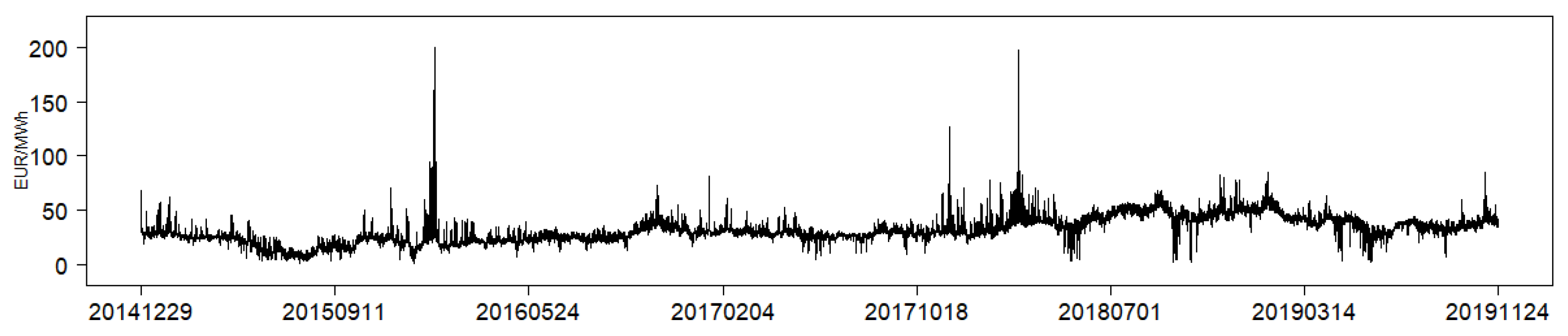
In the Nord Pool power market, the system is balanced using three different markets: day-ahead market (i.e., Elspot, volume 98%), intraday market (i.e., Elbas, volume 1%) and balancing market (volume 1%). In the study, we consider the prices from the market with the highest volume: the day-ahead market. The system price is an unconstrained market clearing reference price. It is calculated without any congestion restrictions by setting capacities to infinity. All orders from Nordic (Denmark, Finland, Norway, Sweden) and Baltic regions (Lithuania, Latvia, Estonia) are included in the system price calculation. Most standard financial contracts traded in the Nordic region use the system price as a reference price. In the paper, we analyse the electricity system price in two periods: between 29 December 2014 and 26 March 2017, which covers hourly observations for 819 days, and between 29 December 2014 and 24 November 2019, which covers hourly observations for 1792 days. The data concern hourly electricity prices from the day-ahead market. The first data set is used in an empirical study to forecast hourly day-ahead electricity prices (see Section 5). Here and in Section 3, we focus on the second data set and explore the main characteristics of electricity price jumps (see Figure 1).

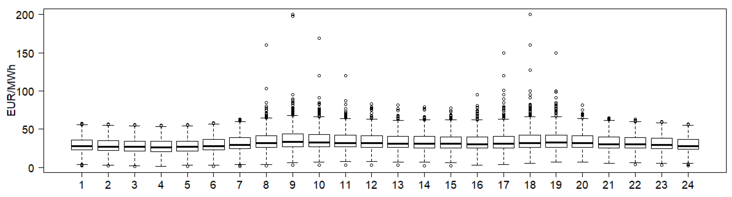
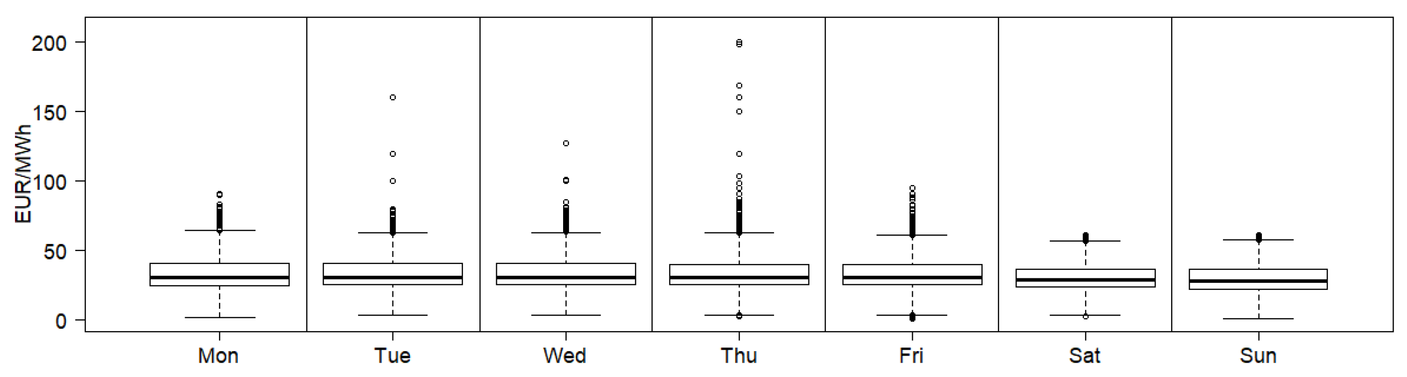
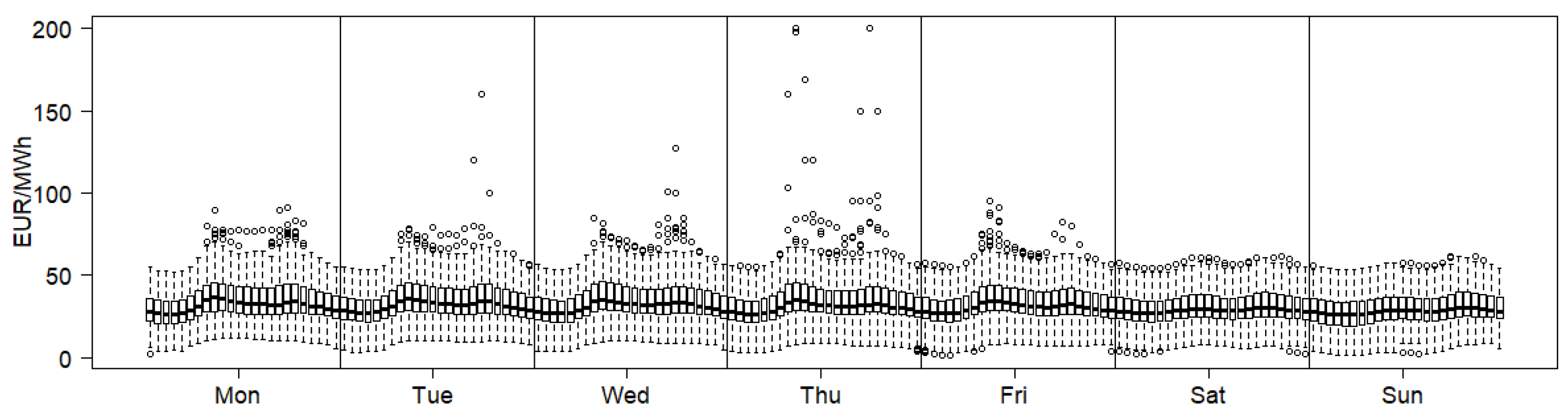
Electricity prices are subject to various kinds of seasonality, e.g., intra-daily and intra-weekly, and this is related to winter and summer. Higher electricity prices can be observed during the hours of increased demand for electricity, on working days and in winter. Figure 2 presents the boxplots of electricity prices for each hour of the day with a typical price volatility pattern, i.e., higher around hours #8–11 and #17–19. A calmer night-time price behaviour can also be observed. Similarly, Figure 3 and Figure 4 present the boxplots for each day and each hour of a week, respectively. Electricity prices on Saturdays and Sundays are lower and calmer (fewer extreme prices) than on working days (Mondays to Fridays). In the analysed period, the prices on Tuesdays and Thursdays are the most volatile. In particular, the jump intensity seems to depend on an hour and the day of the week. Thus, it is worth or even necessary to consider the time-varying intensity of jumps in modelling and forecasting electricity prices. The appropriate incorporation of such information and properties seems to facilitate more precise forecasting of prices.

In the study, we consider also variables connected with the electricity market such as hourly data concerning electricity consumption forecasts, wind power generation forecasts and failures of power plants (lagged by 48 h). We also consider weekly data on the water level in the reservoirs of hydroelectric power plants. The data were downloaded from two websites: nordpoolgroup.com and transparency.entsoe.eu. In case of a time change, we take the average value for neighbouring (spring) or doubled (autumn) hours. In case of missing information, we estimate the value as an average for the neighbouring days at that hour. We use these variables in the models for forecasting electricity prices in Section 5 describing the empirical results.

3. Electricity Price Jump Features

The problem of the unambiguous identification of electricity price jumps has not been solved yet. In the literature, jumps are defined as prices above/below a certain threshold [32,34] or detected similarly as outliers, e.g., by means of the quantile analysis, the recursive filter on prices [36,43], the Tukey criterion [44,45], the adjusted boxplot [46], non-parametric techniques such as that of Barndorff-Nielsen and Shephard [47,48,49,50,51] and Bayesian methods of jump detection [38].

In this part of the paper, we detect jumps by means of three methods: the recursive filter on prices, the Tukey criterion and the adjusted boxplot approach, and we examine the behaviour of price jumps. We detect jumps in 24 electricity price series after removing a short- and long-term seasonality component and a trend using the median filter and the Hodrick-Prescott filter [39,52].

The recursive filter on prices (RFP) treats the prices outside the range determined by the mean plus or minus three standard deviations as jumps. After rejecting the already determined jumps, both the mean and the standard deviation are recalculated and the consecutive jumps are determined. Within the method based on the Tukey criterion (a standard boxplot), the values outside the range $[Q_1-1.5·IQR;Q_3+1.5·IQR]$ are marked as downward and upward jumps [43,44,45], where $Q_1$ and $Q_3$ are the lower and upper quartiles and $IQR=Q_3-Q_1$ is the interquartile range. However, electricity prices tend to have a skewed distribution; thus, we also employ the method based on an adjusted boxplot [46]. Within this method, the values outside the range $[Q_1-1.5·IQR·exp(-4MC);Q_3+1.5·IQR·exp\left(3MC\right)]$ are marked as downward and upward jumps, respectively. The robust measure of the skewness, the medcouple ($MC$), was introduced by Brys et al. [53] (see also [46]) and is defined as $MC=\underset{x_i\le Q_2\le x_j}{median}\frac{(x_j-Q_2)-(Q_2-x_i)}{x_j-x_i}$, where $x_1,\cdots ,x_n$ is a data set and $Q_2$ is a sample median of the set $x_1,\cdots ,x_n$, i.e., $MC$ is calculated as a median of values $\frac{(x_j-Q_2)-(Q_2-x_i)}{x_j-x_i}$ calculated for all $\{(i,j):x_i\le Q_2\le x_j\}$. The described methods do not lead to equivalent results; however, they allow noticing common electricity price jump features regardless of the method used.

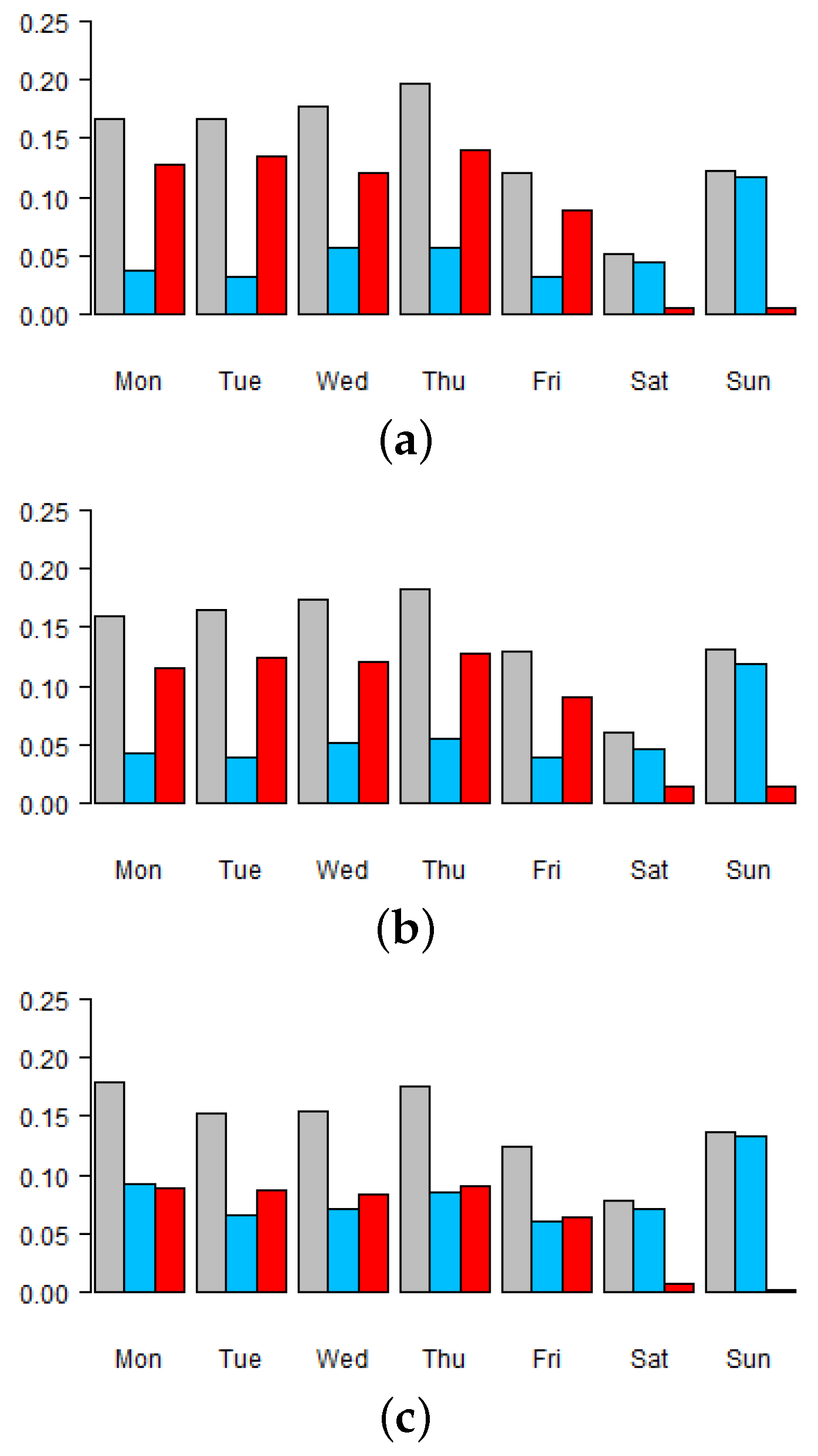
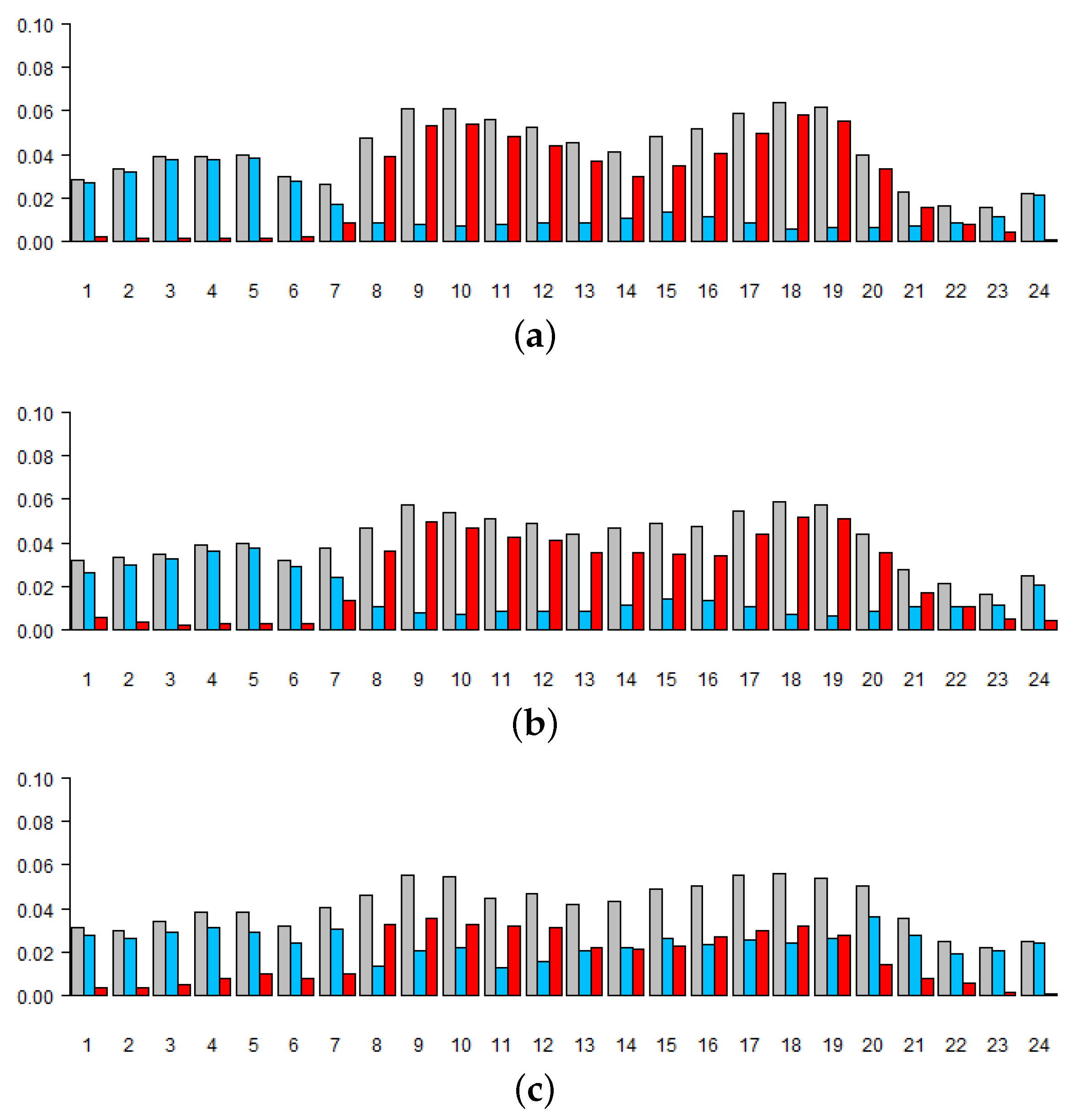
Figure 5 presents the percentage of jumps out of all jumps that occur on each day of the week and are detected by one of the methods. They all lead to the following conclusions: on working days, there are more upward than downward jumps; on Saturdays and Sundays, there are far fewer upward jumps; on Sundays, the percentage of downward jumps is the highest. These results are consistent with the electricity demand pattern. Figure 6 demonstrates the percentage of jumps out of all detected jumps that occur at each hour of the day. In this case as well, there are more jumps, especially upward jumps, in the period of increased demand for electricity, while at night, downward jumps prevail.

Regardless of the detection method applied, the results indicate that the occurrence of electricity price jumps depends on an hour of the day and the day of the week and that the intensity of downward jumps is governed by a different rule than that of upward jumps. The observations are used in the empirical part of our study to forecast downward and upward jump occurrences.

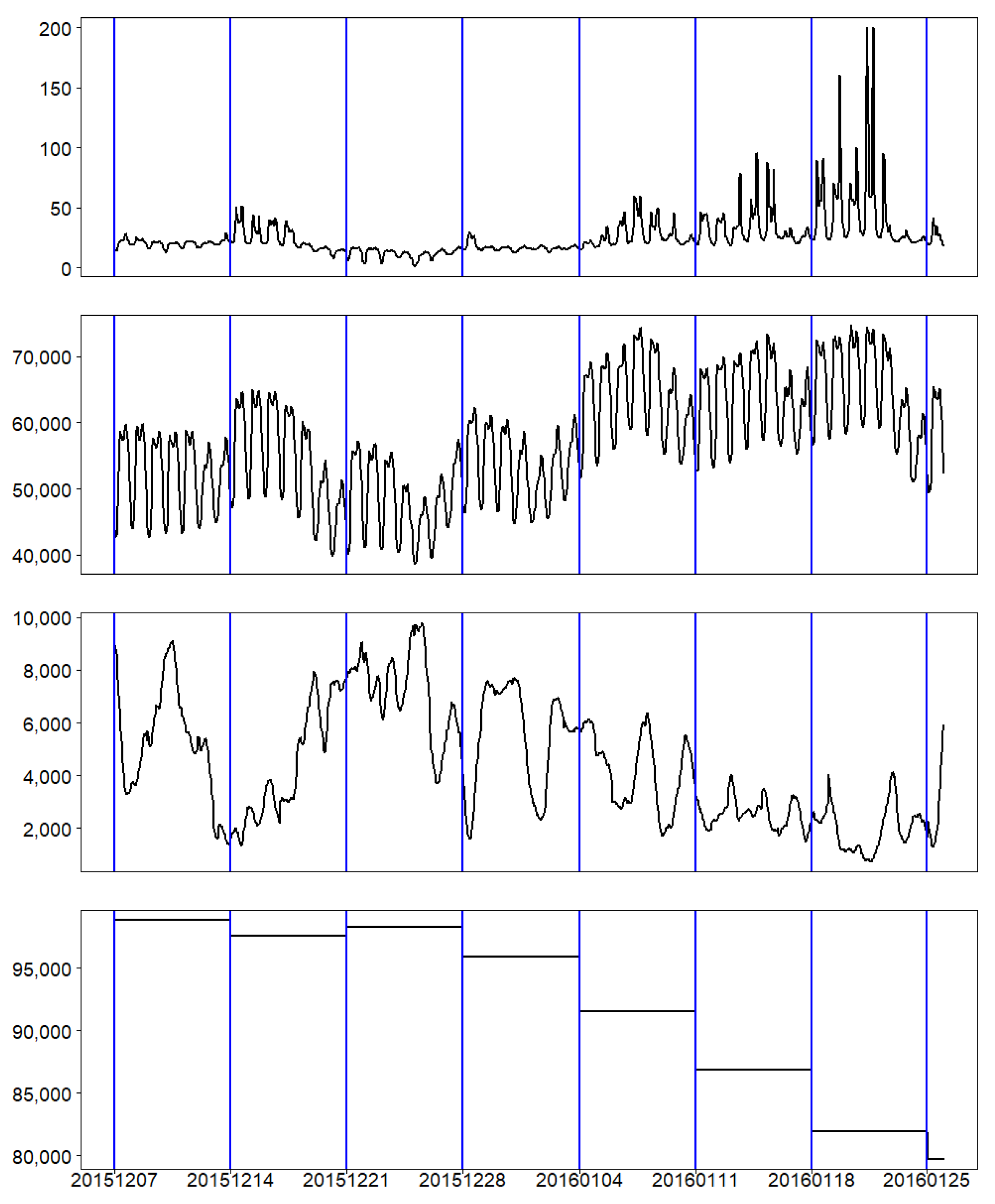
The electricity prices in the day-ahead market are affected by the forecast of wind power generation and the current water level in hydroelectric reservoirs, especially in markets with a high share of renewable energy sources. It can be expected that these factors may also contribute to the occurrence of price shocks. Figure 7 presents the price and electricity consumption forecasts, together with wind power generation forecasts and the water level in hydroelectric reservoirs before the highest price peak at the end of January 2016. Higher prices recorded five weeks earlier were accompanied by higher production and consumption forecasts and the low forecast of wind power generation. The situation had been similar for two weeks preceding the price peak, but the water level in the reservoirs of hydroelectric power plants continued to decline. During the week when the price peak occurred, consumption forecasts still remained at a high level, and both the wind power generation forecasts and the water level were low. That week, the electricity prices reached a level about eight times higher than the average level of Nord Pool electricity prices.

The linkage between the occurrence of price jumps, seasonality and electricity consumption, wind power and water level indicates that these variables should also be included in jump modelling as explanatory variables. Due to the requirement of continuous balancing between electricity production and consumption, power plant failures can also play an important role in price jumps (e.g., [39]).

We employ the generalised ordered logit model for forecasting the occurrence of jumps. The model deals with the probability estimation of the occurrence of ordered outcomes. In our study, the variable describing jumps can take three values:

$$\begin{array}{c}\hfill q_t=\left\{\begin{array}{cc}-1& \mathrm{in}\mathrm{case}\mathrm{of}\mathrm{the}\mathrm{downward}\mathrm{jump}\mathrm{occurrence}\\ 0& \mathrm{in}\mathrm{case}\mathrm{of}\mathrm{no}\mathrm{jump}\mathrm{occurrence}\\ 1& \mathrm{in}\mathrm{case}\mathrm{of}\mathrm{the}\mathrm{upward}\mathrm{jump}\mathrm{occurrence}.\end{array}\right.\end{array}$$

(1)

The generalised ordered logit model for M categories of the dependent variable takes the form [31]:

$$\begin{array}{c}\hfill P(q_t>j|X_t)=\frac{exp({\alpha }_j+{\beta }_{j1}{X}_{1,t}+\dots +{\beta }_{jl}{X}_{l,t})}{1+exp({\alpha }_j+{\beta }_{j1}{X}_{1,t}+\dots +{\beta }_{jl}{X}_{l,t})}\mathrm{for}j=1,\cdots ,M-1,\end{array}$$

(2)

where ${\alpha }_j$ are thresholds, $X_t=(X_{1,t},\cdots ,X_{l,t})$ is a vector of l explanatory variables and ${\beta }_j=({\beta }_{j1},\cdots ,{\beta }_{jl})$ is a vector of parameters (without a constant term). In our study, $M=3$, and the model consists of two equations: the first one describes the probability $P(q_t>-1|X_t)$, while the second one describes the probability $P(q_t>0|X_t)$. Different vectors of parameters ${\beta }_j$ are allowed in each of these equations, thus a different impact of the explanatory variables on the probability of an upward jump and a different impact on the probability of a downward jump occurrence can be taken into account. That is a valuable feature of the generalised ordered logit model due to different patterns of upward, downward or no jump occurrences found in the study.

In order to model and forecast the occurrences of these three events ($M=3$): a downward jump, no jump and an upward jump, we employ the generalised ordered logit model with the following explanatory variables: electricity consumption forecasts, wind power generation forecasts, the water level in the reservoirs of hydroelectric power plants, the minimum price of the previous day, failures of power plants lagged by 48 h and seasonality factors: wintertime and days of the week. As in the case of the price series, we remove a short- and long-term seasonality and trend from the variables that need it. On this basis, we forecast the probability of the occurrence of a particular event. We apply this technique of jump occurrence forecasting within the DEJDXOL model (described below) to capture the dependence between the appearance of jumps and the explanatory variables in order to forecast electricity prices more accurately.

4. Bayesian Models

In our study, we focus on the Bayesian models to forecast electricity prices. Time-varying volatility and jumps are the hallmarks of electricity prices. In order to capture these characteristics, we consider models with jumps and/or stochastic volatility. We apply the jump-diffusion models (DEJDX, DEJDXOL), a stochastic volatility model (SVX), a pooling approach and a stochastic volatility model with jumps (SVDEJX). In order to distinguish between downward and upward jumps, we apply the double exponential distribution of jump sizes. The models are extended by explanatory variables, which carry significant information about time series dynamics and correspond to the typical characteristics of electricity prices.

Let ${\left\{y_t\right\}}_{t=1,\dots ,n}$ denote a log-price (EUR/MWh) at time t, ${\psi }_i\in \mathbb{R}$, $\sigma >0$, ${\sigma }_h>0$, ${\theta }_h\in \mathbb{R}$, ${\kappa }_h\in \left(0,2\right)$, $\rho \in \left(0,1\right)$, variables $X_1$, ..., $X_k$ represent explanatory variables, $\left\{{\epsilon }_t^{\left(1\right)}\right\},\left\{{\epsilon }_t^{\left(2\right)}\right\}\sim iidN\left(0,1\right)$, $\left\{J_t\right\}\sim iid$, $J_t$ represent a value of a jump at t and $J_t$ have a double exponential distribution with a density:

$$\begin{array}{cc}\hfill p_{J_t}\left(x\right)=& p_D\frac{1}{{\eta }_D}exp\left(\frac{1}{{\eta }_D}x\right){\mathbb{I}}_{\left(-\infty ,0\right)}\left(x\right)+p_0{\mathbb{I}}_{\left\{0\right\}}\left(x\right)+\\ \hfill & +p_U\frac{1}{{\eta }_U}exp\left(-\frac{1}{{\eta }_U}x\right){\mathbb{I}}_{\left(0,\infty \right)}\left(x\right),\end{array}$$

(3)

where $p_D\in \left(0,1\right)$, $p_0\in \left(0,1\right)$, $p_U\in \left(0,1\right)$, $p_D+p_0+p_U=1$, ${\eta }_D>0$, ${\eta }_U>0$ and $\mathbb{I}$ stands for an indicator function. The distribution of $J_t$ allows modelling downward and upward jumps separately.

Three out of five considered models are presented as follows:

• The DEJDX model:

  $$\begin{array}{cc}\hfill y_{t+1}=& y_t+{\psi }_1{X}_{1,t+1}+\dots +{\psi }_k{X}_{k,t+1}+\sigma {\epsilon }_{t+1}+J_{t+1}\end{array}$$

  (4)
• The SVX model:

  $$\begin{array}{cc}\hfill y_{t+1}=& y_t+{\psi }_1{X}_{1,t+1}+\dots +{\psi }_k{X}_{k,t+1}+\sqrt{exp\left(h_t\right)}{\epsilon }_{t+1}^{\left(1\right)}\hfill \\ \hfill h_{t+1}=& h_t+{\kappa }_h\left({\theta }_h-h_t\right)+{\sigma }_h\left(\rho {\epsilon }_{t+1}^{\left(1\right)}+\sqrt{1-{\rho }^2}{\epsilon }_{t+1}^{\left(2\right)}\right)\hfill \end{array}$$

  (5)
• The SVDEJX model:

  $$\begin{array}{cc}\hfill y_{t+1}=& y_t+{\psi }_1{X}_{1,t+1}+\dots +{\psi }_k{X}_{k,t+1}+\sqrt{exp\left(h_t\right)}{\epsilon }_{t+1}^{\left(1\right)}+J_{t+1}\hfill \\ \hfill h_{t+1}=& h_t+{\kappa }_h\left({\theta }_h-h_t\right)+{\sigma }_h\left(\rho {\epsilon }_{t+1}^{\left(1\right)}+\sqrt{1-{\rho }^2}{\epsilon }_{t+1}^{\left(2\right)}\right)\hfill \end{array}$$

  (6)

The following are the explanatory variables X’s: the logarithm of electricity consumption forecast, the minimum of the previous day’s hourly log-prices and a dummy variable representing working days. Jumps are modelled under the Bayesian approach as latent variables, which allow the formal inference about the times and sizes of the jump occurrence. The inference within the Bayesian DEJDX model hinges upon the joint density:

$$p\left(y,\theta ,q,\xi \right)=p\left(y\left|\theta ,q,\xi \right.\right)p\left(\theta ,q,\xi \right),$$

(7)

where y is a vector of observed data, $\theta =\left({\eta }_D,{\eta }_U,p_D,p_0,p_U,{\psi }_1,\dots ,{\psi }_k,{\sigma }^2\right)$ is a vector of unknown parameters, $q=\left(q_1,\dots ,q_n\right)$ is a vector of the time occurrence of jumps, $\xi =\left({\xi }_1^D,{\xi }_1^U,\dots ,{\xi }_n^D,{\xi }_n^U\right)$ represents a vector of jump values, ${\xi }_n^D$ represents a downward jump, ${\xi }_n^U$ represents an upward jump, $J_t=-{\xi }_t^D·\mathbb{I}\left(q_t=-1\right)+{\xi }_t^U·\mathbb{I}\left(q_t=1\right)$, $p\left(\theta ,q,\xi \right)$ is a prior density and $p\left(y\left|\theta ,q,\xi \right.\right)$ is a sampling density. The prior structure is defined as $p\left({\eta }_D\right)\sim IG\left(1.86,0.43\right)$, $p\left({\eta }_U\right)\sim IG\left(1.86,0.43\right)$, $\left(p_D,p_0,p_U\right)\sim Dirichlet\left(1,1,1\right)$, ${\psi }_i\sim N\left(0,1\right)$, $p\left({\sigma }^2\right)\sim IG\left(5,1\right)$, $q_t=\left\{\begin{array}{cc}-1& \mathrm{with}\mathrm{probability}{p}_D,\\ 0& \mathrm{with}\mathrm{probability}{p}_0,\\ 1& \mathrm{with}\mathrm{probability}{p}_U,\end{array}\right.$${\xi }_t^D\sim Exp\left({\eta }_D\right)$, ${\xi }_t^U\sim Exp\left({\eta }_U\right)$. The construction of the other Bayesian models is similar to DEJDX.

The occurrence of a jump at t is equivalent to $q_t\ne 0$. The identification of jumps under the Bayesian approach is based on the posterior probability of a jump, $P\left(\left.q_t\ne 0\right|y\right)$. The inference about unknown parameters and latent variables is based on the posterior distribution $p\left(\theta ,q,\xi \left|y\right.\right)$. The posterior distribution is not a standard distribution; therefore, we have to apply the Markov chain Monte Carlo methods [54].

Under the Bayesian approach, the forecasting is determined by the predictive distribution. The distribution handles the uncertainty about unknown parameters, latent variables conditional on previous observations and the assumptions of the model. The Bayesian pooling approach allows combining forecasts calculated under the individual models DEJDX and SVX by means of the predictive Bayes factor [55].

The drawback of the DEJDX model is an assumption of independent times of jump occurrences and a constant intensity of jumps. The attempt to solve this problem is to replace the constant intensity of jumps by the time-varying intensity, which depends on the explanatory variables. For this purpose, we introduce the DEJDXOL model, i.e., the double exponential jump-diffusion model with explanatory variables and the intensity of jump occurrences given by the generalised ordered logit specification described above. We assume:

$$\begin{array}{cc}\hfill y_{t+1}=& y_t+{\psi }_1{X}_{1,t+1}+\dots +{\psi }_k{X}_{k,t+1}+\sigma {\epsilon }_{t+1}+J_{t+1}\hfill \\ \hfill J_{t+1}=& -{\xi }_{t+1}^D·\mathbb{I}\left(q_{t+1}=-1\right)+0·\mathbb{I}\left(q_{t+1}=0\right)+{\xi }_{t+1}^U·\mathbb{I}\left(q_{t+1}=1\right),\hfill \end{array}$$

(8)

where ${\xi }_{t+1}^D\sim Exp\left({\eta }_D\right)$, ${\xi }_{t+1}^U\sim Exp\left({\eta }_U\right)$, $q_{t+1}=\left\{\begin{array}{cc}-1,& \mathrm{downward}\mathrm{jump}\hfill \\ 0,& \mathrm{no}\mathrm{jump}\hfill \\ 1,& \mathrm{upward}\mathrm{jump}\hfill \end{array}\right.$. Probabilities $P(q_t>-1|X_t)$ and $P(q_t>0|X_t)$ are calculated by means of the generalised ordered logit model ($M=3$, $j\in \{-1,0\}$) with explanatory variables $X_t=(X_{1,t},\cdots ,X_{l,t})$ presented in Section 3.

5. Empirical Results

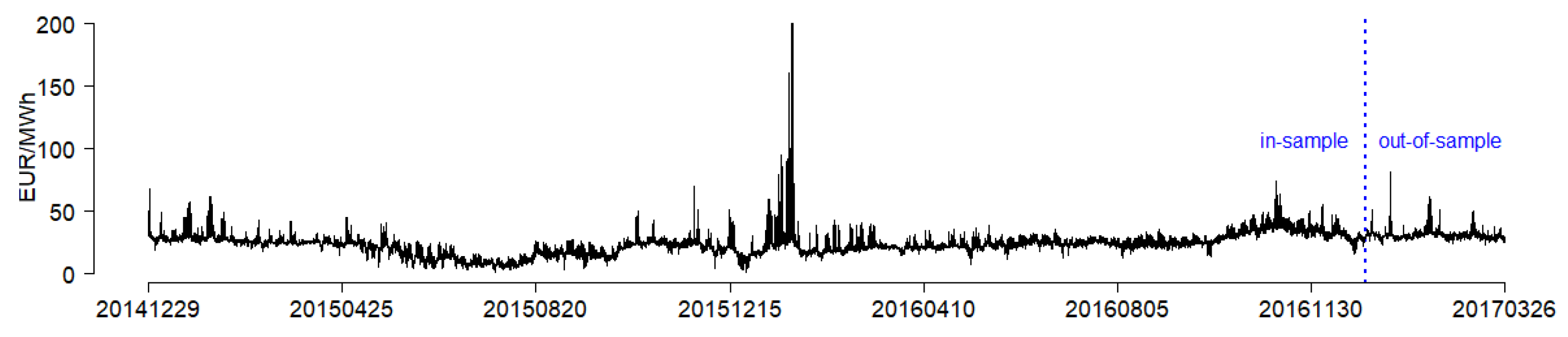
In this part of the study, we focus on forecasting hourly day-ahead electricity prices. We analyse the hourly electricity system price (EUR/MWh) from the Nord Pool market in the period between 29 December 2014 and 26 March 2017. We divide the data set into two subsets. The in-sample set spans the period between 29 December 2014 and 1 January 2017, and the out-of-sample data set spans the period between 2 January 2017 and 26 March 2017 (see Figure 8). We analyse 24 time series of electricity prices separately for each hour of a day.

One of the aims of the study is to compare the results of the electricity price forecasts obtained on the basis of the DEJDX model and the DEJDXOL model introduced above. The former assumes the constant intensity of jumps, while the latter takes into account the changing intensity of jumps by incorporating information from the generalised ordered logit model into the forecasting scheme. For this purpose, we identify downward and upward jumps in the in-sample set by means of the DEJDX model and then employ the generalised ordered logit model to obtain one day-ahead forecasts of the probabilities of downward, no and upward jump occurrences. The forecasts of probabilities are then used within the DEJDXOL model to forecast the electricity price. We repeat the procedure extending the data window by the consecutive observation. Thus, the in-sample period is extended by one observation taken from the out-of-sample period, and the procedure is repeated.

We consider two subsets of explanatory variables. The first one defines the dynamics of log-prices and consists of the electricity consumption forecast, the minimum of the previous day’s hourly log-prices, and a dummy variable for working days. In order to model and forecast the occurrence of downward, no and upward jumps, we employ the generalised ordered logit model with the following set of explanatory variables: electricity consumption forecast, wind power generation forecast, the water level in hydroelectric power plants, the price of the previous day, failures of power plants (lagged by 48 h) and seasonality factors: wintertime and days of the week.

The first day-ahead forecast is calculated under the model estimated using the in-sample data set. The estimation is based on 200,000 MCMC draws, preceded by 1,000,000 burn-in cycles. Subsequent re-estimations, identification of jumps and forecasts are based on data windows extended by a consecutive observation. The re-estimations of the model are based on 20,000 MCMC draws, preceded by 20,000 burn-in cycles. The starting points of the numerical algorithm are set to the medians of the MCMC draws from the previous step, i.e., the starting points are equal to the estimators of posterior medians of the parameters.

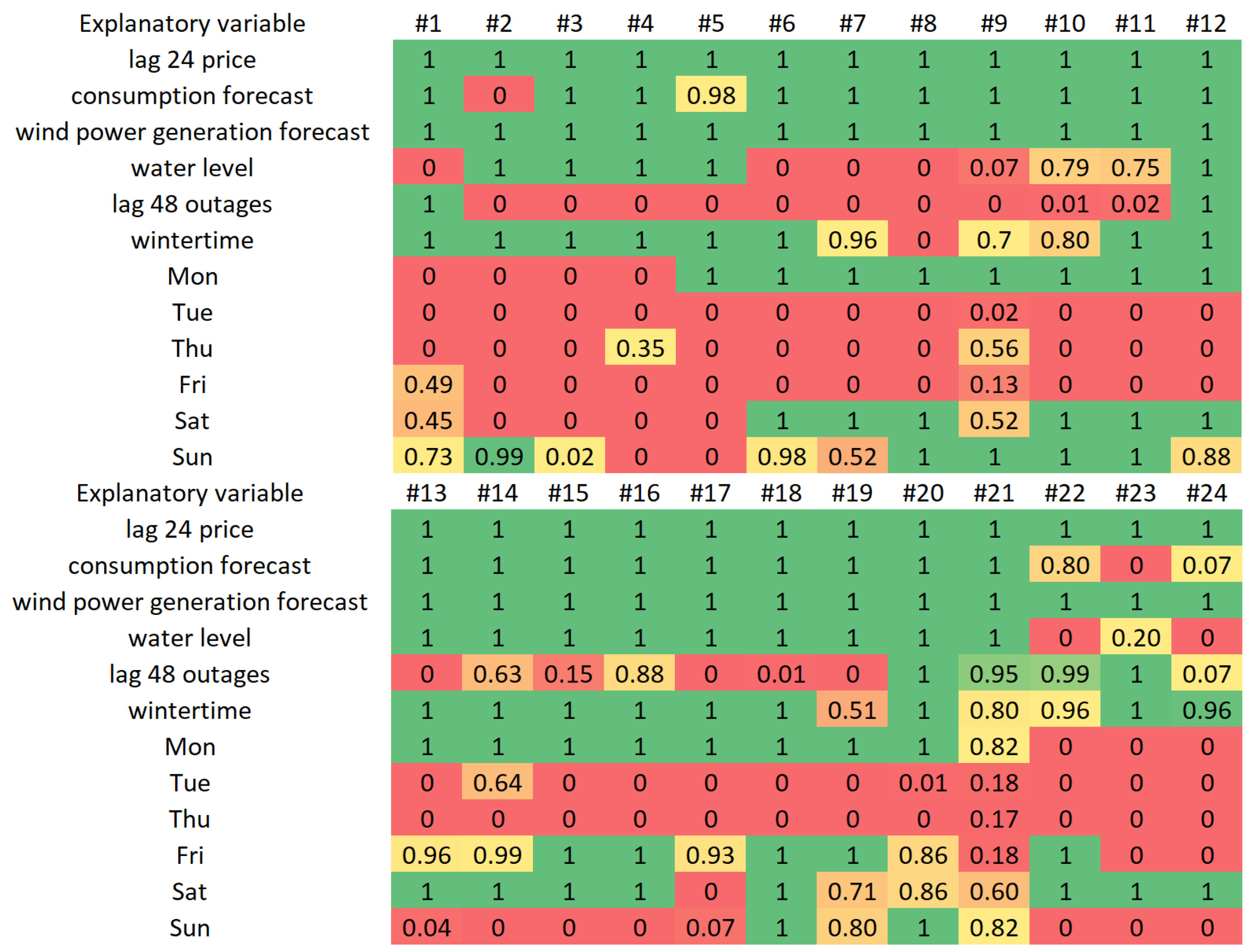
Within the generalised ordered logit model, we examine the statistical significance of the influence of explanatory variables in modelling the intensity of jumps at each hour of the day. This analysis reveals which factors are more likely to affect the probabilities of downward or upward jump occurrences. Figure 9 contains the frequencies with which a variable has a significant influence in the generalised ordered logit models built on the basis of extending data windows. For example, in the case of the consumption forecasts, “1” for hour #1 means it has a significant influence within the models estimated based on all extending windows; “0” for hour #2 means no significant influence in the models; and “0.98” for hour #5 means that within 98% of the models based on extending windows, that variable has a significant influence on the probabilities. Thus, in the case of two variables: the wind power generation forecasts and the price of the previous day, the 1’s for hours #1–24 mean they have a significant influence on the downward/upward jump occurrence probabilities. The consumption forecast has a significant impact on all hours but hours #2 and #23–24. In most cases, the variable outages of power plants lagged by 48 h do not have a significant impact, which suggests a well-diversified and robust electricity production system. The water level, wintertime and the trade on Saturdays have a significant impact for most hours. Furthermore, the trade on Mondays has a significant impact on hours #5–20, which mostly covers the rush hour period. The trade on Fridays is important on hours #13–20 and #22, whilst the trade on Sundays has a significant impact on hours #6–12 and #18–21. That means that the probabilities of jump occurrences differ over days of the week and hours of the day, which corresponds to the jump features described in Section 3.

Table 1. The mean absolute percentage errors (MAPEs) (%) calculated within the DEJDX, SVX, pooling, SVDEJX and DEJDXOL models for each hour of the day in the out-of-sample period (2 January 2017–26 March 2017). The best results for each hour are in bold.

Hour	DEJDX	SVX	Pooling	SVDEJX	DEJDXOL
#1	4.798	4.798	4.776	4.777	4.708
#2	5.172	5.173	5.132	5.107	4.625
#3	5.264	5.263	5.221	5.208	4.559
#4	5.256	5.165	5.158	5.119	4.521
#5	4.822	4.68	4.689	4.678	4.155
#6	4.64	4.471	4.493	4.461	4.157
#7	5.487	5.126	5.177	5.3	4.656
#8	9.32	9.088	9.202	9.346	7.089
#9	11.453	11.484	11.48	11.105	8.999
#10	10.276	10.187	10.24	9.948	8.572
#11	9.224	9.007	9.149	8.872	7.822
#12	7.66	7.462	7.551	7.389	6.918
#13	6.978	6.78	6.873	6.763	6.253
#14	6.652	6.518	6.595	6.486	5.92
#15	6.506	6.438	6.453	6.459	5.837
#16	6.177	6.115	6.138	6.14	5.557
#17	7.503	7.386	7.408	7.428	6.863
#18	9.469	9.347	9.411	9.344	8.297
#19	8.252	8.167	8.203	8.224	7.117
#20	5.368	5.27	5.3	5.308	4.911
#21	4.008	3.931	3.93	3.958	3.81
#22	3.73	3.644	3.667	3.645	3.553
#23	3.675	3.569	3.608	3.555	3.402
#24	4.279	4.257	4.259	4.248	4.187

presents the mean absolute percentage error MAPE based on point forecasts equal to the medians of predictive distributions calculated under the DEJDX, SVX, SVDEJX and DEJDXOL models and the pooling approach. The lower the MAPE, the better the point forecast is. The best results for each hour are in bold. For all hours, the best results are yielded by the jump-diffusion model with a time-varying intensity of jumps (DEJDXOL). In particular, the results calculated under the DEJDXOL model are better than those under the model with a constant jump intensity (DEJDX).

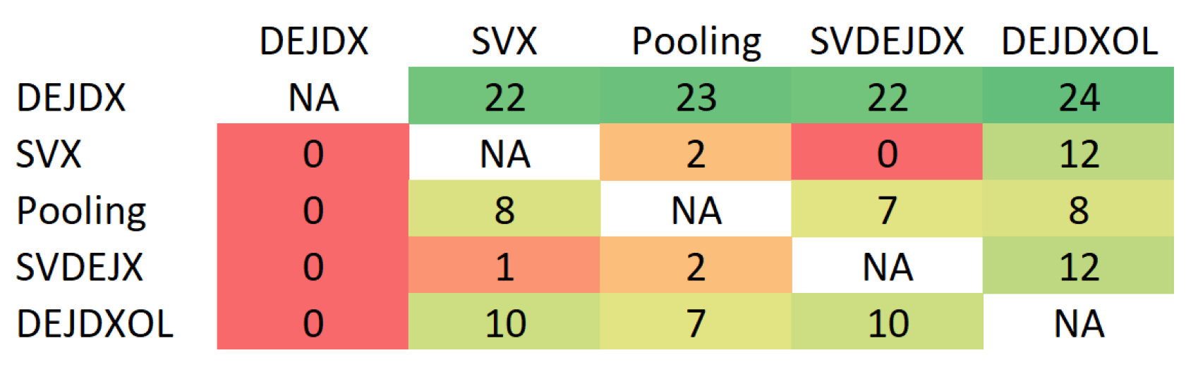
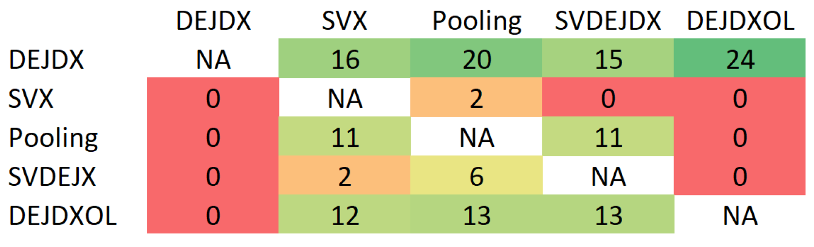
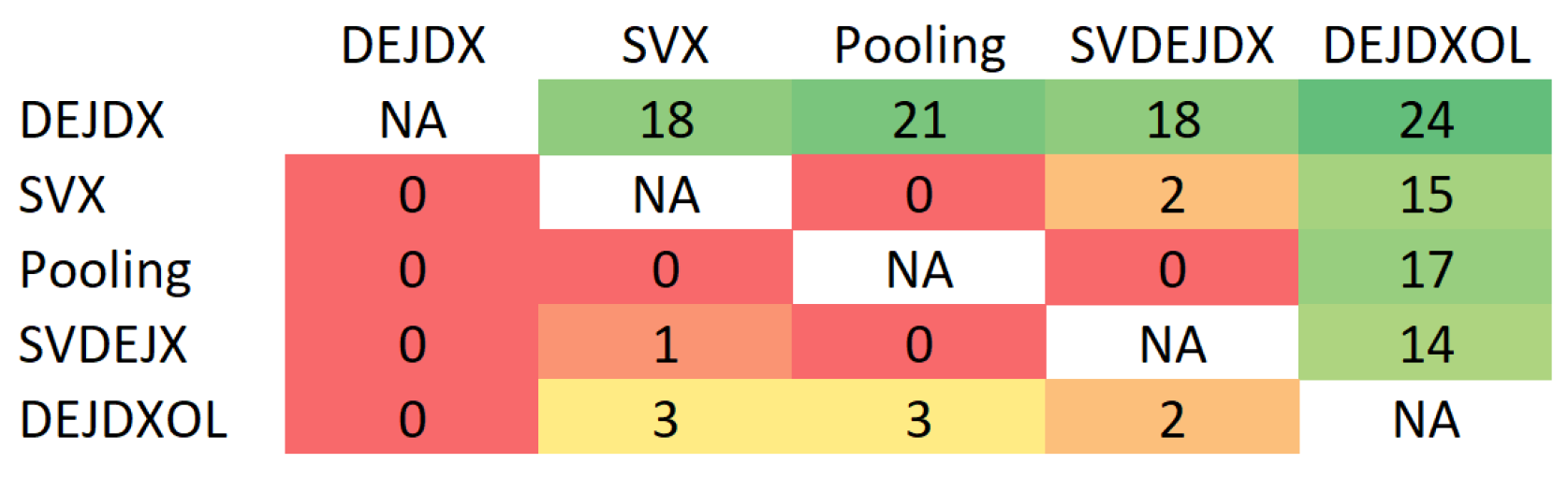
In order to verify whether the probabilistic forecasts calculated within one model are significantly better than the results yielded by the other model, we apply the Diebold-Mariano test [2,56,57]. We employ the pinball loss as a scoring rule for the Diebold-Mariano test. The pinball loss function is a measure of fit for a predictive quantile [2,58]. In the study, the pinball loss for a day and an hour is the average of the pinball loss across 99 quantiles ($0.01,0.02,\dots ,0.99$). Moreover, we conduct the tests based on the pinball loss across $0.01,0.02,\dots ,0.05$ and $0.95,0.96,\dots ,0.99$ quantiles (pinball 10% tails) and across $0.25,0.26,\dots ,0.75$ quantiles (pinball 50% middle). The results of the Diebold-Mariano tests are presented in Figure 10, Figure 11 and Figure 12, which demonstrate the number of hours of the day for which forecasts obtained within a model from the horizontal axis are better than the ones within a model from the vertical axis at a significance level $0.05$.

The probabilistic forecasts calculated within the DEJDXOL model are significantly better than those calculated within the jump-diffusion model DEJDX for hours #1–24 (24 time series) and each of the tests. None of the models is better than the others for each hour. However, we can compare the number of hours for which forecasts of a given model are more accurate than those of the other model. The SVDEJX model is significantly better than the pooling approach for a larger number of hours. The results for the SVX and SVDEJX models are very similar. However, we prefer the simpler structure, that is the SVX model. Eventually, the results indicate that the models with time-varying volatility SVX and the time-varying intensity of jumps DEJDXOL yield the most accurate forecasts. It is impossible to identify a decisive winner between these two models. The results of the pinball $10\%$ tails tests support the SVX model over DEJDXOL (see Figure 11). However, the reverse conclusion might be drawn when analysing the pinball $50\%$ tests (see Figure 12). On the other hand, the number of hours for which one of these models is better than the other one is similar in the case of the (general) pinball tests (see Figure 10). Thus, it is difficult to determine a decisive winner based on these results. That is why we undertake further analyses, whose results are presented below.

Table 2. The results of the Diebold-Mariano tests with the pinball scoring rule at a significance level of 0.05 separately for each hour of the day in the out-of-sample period (2 January 2017–26 March 2017).

	Pinball 50% Middle		Pinball 10% Tails		Pinball
Hour	SVX	DEJDXOL	SVX	DEJDXOL	SVX	DEJDXOL
#1	0	0	1	0	1	0
#2	0	1	1	0	1	0
#3	0	1	1	0	1	0
#4	0	1	1	0	1	0
#5	0	0	1	0	1	0
#6	0	0	1	0	1	0
#7	0	0	1	0	0	0
#8	0	1	1	0	0	1
#9	0	1	0	0	0	1
#10	0	1	0	0	0	1
#11	0	1	0	0	0	1
#12	0	1	0	0	0	1
#13	0	1	0	0	0	1
#14	0	1	0	0	0	1
#15	0	1	0	0	0	1
#16	0	1	0	0	0	1
#17	0	1	0	0	0	1
#18	0	1	0	0	0	1
#19	0	1	0	0	0	1
#20	0	0	0	0	0	0
#21	0	0	1	0	1	0
#22	1	0	1	0	1	0
#23	1	0	1	0	1	0
#24	1	0	1	0	1	0
TOTAL	3	15	12	0	10	12

presents the results of the Diebold-Mariano tests at a significance level of 0.05 and the pinball scoring rule separately for each hour of the day in the SVX and DEJDXOL models. The 1’s mean the probabilistic forecasts of one model are significantly better than the other’s, and 0’s mean they are not better, i.e., they are of the same quality. We compare the model with time-varying volatility SVX and the model with time-varying intensity of jumps DEJDXOL. Similar results (not presented in the paper) are obtained for the conditional predictive ability tests of Giacomini and White [59]. The main conclusion is that the SVX model has an advantage over DEJDXOL primarily in the case of off-peak hours, whilst the DEJDXOL model is better mainly in the case of peak hours. This is in line with the idea of using different models for different time series, i.e., hours. The analysis suggests that the model with time-varying volatility performs better in the case of calmer price series; however, allowing for the time-varying intensity of jumps provides better probabilistic forecasts in the case of time series with sharper and sudden changes of prices.

6. Conclusions and Remarks

In the paper, we use the following Bayesian models: the jump-diffusion model, the stochastic volatility model, the pooling approach, which combines forecasts of the first two models, and the generalised version of the first two models. The models are extended by including explanatory variables. Moreover, we introduce the jump-diffusion model with explanatory variables and a time-varying intensity of jumps and a mechanism of jump prediction (DEJDXOL) and focus on the point and probabilistic forecasts of electricity prices in the day-ahead Nord Pool market from the perspective of the existence of jumps.

First, we discuss the dynamics of electricity prices and the behaviour of price jumps. We use three jump detection methods: the recursive filter on prices, the Tukey criterion and the adjusted boxplot approach, and consider three outcomes: the downward jump, no jump or the upward jump occurrence. In particular, our first conclusion is that the intensity of downward jumps is governed by a different rule than that of upward jumps. The intensity of electricity price jumps, downward and upward, varies over time and depends on certain factors. The finding is supported by the results obtained regardless of the detection method used. Thus, the assumption of the constant jump intensity under the jump-diffusion model is not confirmed empirically.

The above conclusion leads us to describe the time-varying intensity of jumps using the generalised ordered logit model. The advantage of the model lies in offering the possibility to consider a different influence of explanatory variables on the probabilities of the downward, no or upward jump occurrence. This is in line with different rules of downward and upward jump formation observed in the study. Our results reveal explanatory variables essential for forecasting the moments of jump occurrences.

Taking the above findings into account, we apply the jump probability forecasts obtained by means of the generalised ordered logit model within the DEJDXOL model to forecast electricity prices. The results indicate that the jump-diffusion model with explanatory variables, a time-varying intensity of jumps and a mechanism of jump prediction, i.e., the DEJDXOL model, is better than the jump-diffusion model with explanatory variables and a constant intensity of jumps (DEJDX). Therefore, we conclude that models with jumps should be improved by a time-varying intensity of jumps and a mechanism of jump prediction. Our results are consistent with the works of Seifert and Uhrig-Homburg [26] and Diewald et al. [24]. Moreover, the stochastic volatility model with explanatory variables (SVX) is superior to the DEJDXOL model in the case of off-peak hours, although the DEJDXOL model is better in the case of peak hours. This is consistent with the hypothesis that there is no ideal model and supports the legitimacy of the idea of using different models for off-peak hours and different ones for peak hours. The finding is similar to the conclusion drawn in the work of Chen and Bunn [60] who used the logistic smooth transition regression models with different sets of explanatory variables to analyse UK electricity spot prices in different (half-hourly) trading periods. It is worth emphasising that the DEJDXOL model, which incorporates the information about downward/upward jump occurrence probabilities, gives better forecasts of electricity prices in a more volatile period.

The conclusions drawn in the paper are based on the study of a certain market and prices over a certain period of time. However, the example of the application of the jump-diffusion model with explanatory variables and a mechanism of jump prediction demonstrates that the model could be useful for forecasting day-ahead electricity prices, especially in the case of peak-hours, in other electricity markets where we also observe different dependence of downward and upward jumps on explanatory variables. In further research, we plan to combine the electricity price forecasts of DEJDXOL and SVX by means of the pooling approach.

References

- Weron, R. Electricity Price Forecasting: A Review of the State-of-the-art with a Look into the Future. Int. J. Forecast. 2014, 30, 1030–1081. [Google Scholar] [CrossRef] [Green Version]
- Nowotarski, J.; Weron, R. Recent Advances in Electricity Price Forecasting: A Review of Probabilistic Forecasting. Renew. Sustain. Energy Rev. 2018, 81, 1548–1568. [Google Scholar] [CrossRef]
- Hong, T.; Pinson, P.; Wang, Y.; Weron, R.; Yang, D.; Zareipour, H. Energy Forecasting: A Review and Outlook. IEEE Open Access J. Power Energy 2020, 7, 376–388. [Google Scholar] [CrossRef]
- Thompson, M.; Davison, M.; Rasmussen, H. Valuation and Optimal Operation of Electric Power Plants in Competitive Markets. Oper. Res. 2004, 52, 546–562. [Google Scholar] [CrossRef]
- Kanamura, T.; Ōhashi, K. A Structural Model for Electricity Prices with Spikes: Measurement of Spike Risk and Optimal Policies for Hydropower Plant Operation. Energy Econ. 2007, 29, 1010–1032. [Google Scholar] [CrossRef]
- Uniejewski, B.; Weron, R.; Ziel, F. Variance Stabilizing Transformations for Electricity Spot Price Forecasting. IEEE Trans. Power Syst. 2018, 33, 2219–2229. [Google Scholar] [CrossRef] [Green Version]
- Zareipour, H.; Canizares, C.A.; Bhattacharya, K. Economic Impact of Electricity Market Price Forecasting Errors: A Demand-side Analysis. IEEE Trans. Power Syst. 2010, 25, 254–262. [Google Scholar] [CrossRef]
- Weron, R. Modeling and Forecasting Electricity Loads and Prices. A Statistical Approach; John Wiley & Sons Ltd.: Hoboken, NJ, USA, 2006. [Google Scholar]
- Jacquier, E.; Polson, N.; Rossi, P. Bayesian Analysis of Stochastic Volatility Models. J. Bus. Econ. Stat. 1994, 12, 371–389. [Google Scholar]
- Pajor, A. Procesy Zmienności Stochastycznej SV w Bayesowskiej Analizie Finansowych Szeregów Czasowych; Wydawnictwo Akademii Ekonomicznej w Krakowie: Krakow, Poland, 2003. (In Polish) [Google Scholar]
- Jacquier, E.; Polson, N.; Rossi, P. Bayesian Analysis of Stochastic Volatility Models with Fat-tails and Correlated Errors. J. Econom. 2004, 122, 185–212. [Google Scholar] [CrossRef]
- Yu, J. On Leverage in a Stochastic Volatility Model. J. Econom. 2005, 127, 165–178. [Google Scholar] [CrossRef]
- Omori, Y.; Chib, S.; Shephard, N.; Nakajima, J. Stochastic Volatility with Leverage: Fast and Efficient Likelihood Inference. J. Econom. 2007, 140, 425–449. [Google Scholar] [CrossRef] [Green Version]
- Eraker, B.; Johannes, M.; Polson, N. The Impact of Jumps in Volatility and Returns. J. Financ. 2003, 1269–1300. [Google Scholar] [CrossRef]
- Black, F.; Scholes, M. The Pricing of Options and Corporate Liabilities. J. Political Econ. 1973, 81, 637–654. [Google Scholar] [CrossRef] [Green Version]
- Merton, R.C. Option Pricing when Underlying Stock Return Rates are Discontinuous. J. Financ. Econ. 1976, 3, 125–144. [Google Scholar] [CrossRef] [Green Version]
- Heston, S.L. A Closed-Form Solution for Options with Stochastic Volatility with Applications to Bond and Currency Options. Rev. Financ. Stud. 1993, 6, 327–343. [Google Scholar] [CrossRef] [Green Version]
- Bates, D.S. Jumps and Stochastic Volatility: Exchange Rate Processes Implicit in Deutsche Mark Options. Rev. Financ. Stud. 1996, 9, 69–107. [Google Scholar] [CrossRef]
- Chib, S.; Nardari, F.; Shephard, N. Markov Chain Monte Carlo Methods for Stochastic Volatility Models. J. Econom. 2002, 108, 281–316. [Google Scholar] [CrossRef]
- Li, H.; Wells, M.; Yu, C. A Bayesian Analysis of Return Dynamics with Levy Jumps. Rev. Financ. Stud. 2008, 21, 2345–2378. [Google Scholar] [CrossRef]
- Szerszen, P. Bayesian Analysis of Stochastic Volatility Models with Levy Jumps: Application to Risk Analysis; Finance and Economics Discussion Series Divisions of Research & Statistics and Monetary Affairs Federal Reserve Board: Washington, DC, USA, 2009; pp. 1–52.
- Johannes, M.; Polson, N. MCMC Methods for Continuous-Time Financial Econometrics. In Handbook of Financial Econometrics: Applications; Elsevier: Amsterdam, The Netherlands, 2010; pp. 1–72. [Google Scholar]
- Brooks, C.; Prokopczuk, M. The Dynamics of Commodity Prices. Quant. Financ. 2013, 13, 527–542. [Google Scholar] [CrossRef]
- Diewald, L.; Prokopczuk, M.; Simen, C.W. Time-variations in Commodity Price Jumps. J. Empir. Financ. 2015, 31, 72–84. [Google Scholar] [CrossRef]
- Kostrzewski, M.; Kostrzewska, J. Probabilistic Electricity Price Forecasting with Bayesian Stochastic Volatility Models. Energy Econ. 2019, 80, 610–620. [Google Scholar] [CrossRef]
- Seifert, J.; Uhrig-Homburg, M. Modelling Jumps in Electricity Prices: Theory and Empirical Evidence. Rev. Deriv. Res. 2007, 10, 59–85. [Google Scholar] [CrossRef]
- Kou, S.; Yu, C.; Zhong, H. Jumps in Equity Index Returns Before and During the Recent Financial Crisis: A Bayesian Analysis. Manag. Sci. 2017, 63, 988–1010. [Google Scholar] [CrossRef] [Green Version]
- Box, G.E.; Tiao, G.C. Bayesian Inference in Statistical Analysis; Addison-Wesley Publishing Company: Boston, MA, USA, 1973. [Google Scholar]
- Bernardo, J.M.; Smith, A.F. Bayesian Theory; John Wiley & Sons: Hoboken, NJ, USA, 2009. [Google Scholar]
- Kostrzewski, M. Bayesian DEJD Model and Detection of Asymmetry in Jump Sizes. Cent. Eur. J. Econ. Model. Econom. 2015, 7, 43–70. [Google Scholar]
- Williams, R. Generalized Ordered Logit/Partial Proportional Odds Models for Ordinal Dependent Variables. Stata J. 2006, 6, 58–82. [Google Scholar] [CrossRef] [Green Version]
- Christensen, T.; Hurn, A.; Lindsay, K. Forecasting Spikes in Electricity Prices. Int. J. Forecast. 2012, 28, 400–411. [Google Scholar] [CrossRef]
- Eichler, M.; Grothe, O.; Manner, H.; Tuerk, D. Modeling Spike Occurrences in Electricity Spot Prices for Forecasting; METEOR, Maastricht University School of Business and Economics: Maastricht, The Netherlands, 2012. [Google Scholar]
- Eichler, M.; Grothe, O.; Manner, H.; Dennis, T. Models for Short-term Forecasting of Spike Occurrences in Australian Electricity Markets: A Comparative Study. J. Energy Mark. 2014, 7, 55–81. [Google Scholar] [CrossRef] [Green Version]
- Hellström, J.; Lundgren, J.; Yu, H. Why Do Electricity Prices Jump? Empirical Evidence from the Nordic Electricity Market. Energy Econ. 2012, 34, 1774–1781. [Google Scholar] [CrossRef]
- Janczura, J.; Trück, S.; Weron, R.; Wolff, R. Identifying Spikes and Seasonal Components in Electricity Spot Price Data: A Guide to Robust Modeling. Energy Econ. 2013, 38, 96–110. [Google Scholar] [CrossRef] [Green Version]
- Kostrzewski, M. On the Existence of Jumps in Financial Time Series. Acta Phys. Pol. 2012, 43, 2001–2019. [Google Scholar] [CrossRef]
- Kostrzewski, M. The Bayesian Methods of Jump Detection: The Example of Gas and EUA Contract Prices. Cent. Eur. J. Econ. Model. Econom. 2019, 11, 107–131. [Google Scholar]
- Kostrzewska, J.; Kostrzewski, M. The Logistic Regression in Predicting Spike Occurrences in Electricity Prices. In Proceedings of the 12th Professor Aleksander Zelias International Conference on Modelling and Forecasting of Socio-Economic Phenomena: Conference Proceedings; Papież, M., Śmiech, S., Eds.; Foundation of the Cracow University of Economics: Cracow, Poland, 2018; pp. 219–228. [Google Scholar]
- Kostrzewski, M. Bayesian SVLEDEJ Model for Detecting Jumps in Logarithmic Growth Rates of One Month Forward Gas Contract Prices. Cent. Eur. J. Econ. Model. Econom. 2016, 8, 161–179. [Google Scholar]
- Morales, L.; Hanly, J. European Power Markets—A Journey Towards Efficiency. Energy Policy 2018, 116, 78–85. [Google Scholar] [CrossRef]
- Papaioannou, G.P.; Dikaiakos, C.; Stratigakos, A.C.; Papageorgiou, P.C.; Krommydas, K.F. Testing the Efficiency of Electricity Markets Using a New Composite Measure Based on Nonlinear TS Tools. Energies 2019, 12, 618. [Google Scholar] [CrossRef] [Green Version]
- Kostrzewska, J.; Kostrzewski, M.; Pawełek, B.; Gałuszka, K. The Classical and Bayesian Logistic Regression in the Research on the Financial Standing of Enterprises after Bankruptcy in Poland. In Proceedings of the 10th Professor Aleksander Zeliaś International Conference on Modelling and Forecasting of Socio-Economic Phenomena: Conference Proceedings; Papież, M., Śmiech, S., Eds.; Foundation of the Cracow University of Economics: Cracow, Poland, 2016; pp. 72–81. [Google Scholar]
- Tukey, J.W. Exploratory Data Analysis; Addison-Wesley: Reading, UK, 1977. [Google Scholar]
- Pawełek, B.; Kostrzewska, J.; Lipieta, A. The Problem of Outliers in the Research on the Financial Standing of Construction Enterprises in Poland. In Proceedings of the 9th Professor Aleksander Zeliaś International Conference on Modelling and Forecasting of Socio-Economic Phenomena: Conference Proceedings; Papież, M., Śmiech, S., Eds.; Foundation of the Cracow University of Economics: Cracow, Poland, 2015; pp. 164–173. [Google Scholar]
- Hubert, M.; Vandervieren, E. An Adjusted Boxplot for Skewed Distributions. Comput. Stat. Data Anal. 2008, 52, 5186–5201. [Google Scholar] [CrossRef]
- Barndorff-Nielsen, O.E.; Shephard, N. Power and Bipower Variation with Stochastic Volatility and Jumps. J. Financ. Econom. 2004, 2, 1–37. [Google Scholar] [CrossRef] [Green Version]
- Barndorff-Nielsen, O.E.; Shephard, N. Impact of Jumps on Returns and Realised Variances: Econometric Analysis of Time-Deformed Levy Processes. J. Econom. 2006, 131, 217–252. [Google Scholar] [CrossRef] [Green Version]
- Barndorff-Nielsen, O.E.; Shephard, N. Econometrics of Testing for Jumps in Financial Economics Using Bipower Variation. J. Financ. Econom. 2006, 4, 1–30. [Google Scholar] [CrossRef]
- Ane, T.; Metais, C. Jump Distribution Characteristics: Evidence from European Stock Markets. Int. J. Bus. Econ. 2010, 9, 1–22. [Google Scholar]
- Nguyen, D.B.B.; Prokopczuk, M. Jumps in Commodity Markets. J. Commod. Mark. 2019, 13, 55–70. [Google Scholar] [CrossRef]
- Weron, R.; Zator, M. A Note on Using the Hodrick–Prescott Filter in Electricity Markets. Energy Econ. 2015, 48, 1–6. [Google Scholar] [CrossRef] [Green Version]
- Brys, G.; Hubert, M.; Struyf, A. A Robust Measure of Skewness. J. Comput. Graph. Stat. 2004, 13, 996–1017. [Google Scholar] [CrossRef]
- Gamerman, D.; Lopes, H.F. Markov Chain Monte Carlo. Stochastic Simulation for Bayesian Inference; Chapman & Hall/CRC: Boca Raton, FL, USA, 2006. [Google Scholar]
- Geweke, J.; Amisano, G. Comparing and Evaluating Bayesian Predictive Distributions of Asset Returns. Int. J. Forecast. 2010, 26, 216–230. [Google Scholar] [CrossRef]
- Diebold, F.X.; Mariano, R.S. Comparing Predictive Accuracy. J. Bus. Econ. Stat. 1995, 13, 253–263. [Google Scholar]
- Diebold, F.X. Comparing Predictive Accuracy, Twenty Years Later: A Personal Perspective on the Use and Abuse of Diebold-Mariano Tests. J. Bus. Econ. Stat. 2015, 33, 1–9. [Google Scholar] [CrossRef] [Green Version]
- Maciejowska, K.; Nowotarski, K. A Hybrid Model for GEFCom2014 Probabilistic Electricity Price Forecasting. Int. J. Forecast. 2016, 32, 1051–1056. [Google Scholar] [CrossRef] [Green Version]
- Giacomini, R.; White, H. Tests of Conditional Predictive Ability. Econometrica 2006, 74, 1545–1578. [Google Scholar] [CrossRef] [Green Version]
- Chen, D.; Bunn, D.W. Analysis of the Nonlinear Response of Electricity Prices to Fundamental and Strategic Factors. IEEE Trans. Power Syst. 2010, 25, 595–606. [Google Scholar] [CrossRef]
Figure 1.
The system price in the Nord Pool day-ahead market in the period between 29 December 2014 and 24 November 2019.
Figure 2.
Boxplots of the electricity price for each hour of the day (29 December 2014–24 November 2019).
Figure 3.
Boxplots of the electricity price for each day of the week (29 December 2014–24 November 2019).
Figure 4.
Boxplots of the electricity price for each hour of the week (29 December 2014–24 November 2019).
Figure 5.
Percentage of electricity price jumps (total in grey, downward in blue, upward in red) on each day of the week detected using: (a) the RFP method, (b) the Tukey method and (c) the adjusted boxplot method, for 24 price series separately (29 December 2014–24 November 2019).
Figure 6.
Percentage of electricity price jumps (total in grey, downward in blue, upward in red) at each hour of the day detected using: (a) the RFP method, (b) the Tukey method and (c) the adjusted boxplot method, for 24 price series separately (29 December 2014–24 November 2019).
Figure 7.
The day-ahead electricity prices, electricity consumption forecasts, wind power generation forecasts and the current water level in hydroelectric reservoirs (7 December 2015–25 January 2016).
Figure 8.
The system price in the Nord Pool day-ahead market in the period 29 December 2014–26 March 2017.
Figure 9.
The frequencies with which a variable has a significant influence in the generalised ordered logit models built for hours #1–24 on the basis of extending data windows in the period 29 December 2014–26 March 2017.
Figure 10.
The results of the Diebold-Mariano tests at a significance level of 0.05 and for 24 h of the day with the pinball scoring rule in the out-of-sample period (2 January 2017–26 March 2017).
Figure 11.
The results of the Diebold-Mariano tests at a significance level of 0.05 and for 24 h of the day with the pinball tails scoring rule in the out-of-sample period (2 January 2017–26 March 2017).
Figure 12.
The results of the Diebold-Mariano tests at a significance level of 0.05 and for 24 h of the day with the pinball middle scoring rule in the out-of-sample period (2 January 2017–26 March 2017).