1. Introduction
In the solar energy sector, photovoltaic (PV) technologies showed significant reduction in installation and operation costs, that the levelized cost of electricity (LCOE) averaged at less than 50 €/MWh in 2016 with a net globally installed capacity of 300 GW. However, PV, and also wind power, are highly intermittent sources of electricity that strongly depend on the instantaneous solar irradiance or wind speed, respectively. The prices increase drastically if a separate electric energy storage system is added, rendering the system neither economically nor technologically feasible [
1]. As the portion of such electricity sources increases in the energy system, problems with flexibility and dispatchability become more prominent [
2].
On the other hand, introducing concentrated solar power (CSP), also known as solar thermal energy (STE), in the energy mix offers a feasible solution for such problems [
3,
4]. Despite the higher cost of electricity production by CSP as compared to PV, with recent CSP projects under construction for an LCOE of 120 €/MWh and the most recent tender for the world’s largest CSP project in Dubai for 73 €/MWh [
5], CSP remains economically attractive. This is due to the cost-effective energy storage in the form of thermal energy, which enables the production of dispatchable electric power during different periods of the day [
6]. This adds a significant value to the technology as the share of intermittent renewable energy sources is increased in the electricity generation mix [
7]. For example, the 50 MW CSP plant in Bokpoort in South Africa was reported to have operated for 161 h continuously in March 2016 [
8]. Furthermore, CSP has the lead in process heat applications to economically and environmentally-friendly supply heat to industrial processes [
9].
With the global installed CSP capacity of only 4.8 GW in 2017, which is nearly two orders of magnitude lower than PV [
10], there exists a tremendous margin for cost reduction. This can be achieved by improving the production process through economies of scale and by increasing the system efficiency [
11]. Fostering the system efficiency involves not only improving component efficiencies, but also maximizing the collected solar energy. This can be achieved by optimizing the power plant operation where solar field simulation tools could play an essential role.
CSP power plants are based on concentrating the solar radiation that falls on a large surface area of mirrors on a much smaller one called absorber. This results in very high energy densities that are transformed to thermal energy through absorber layers on the tubes. A heat transfer fluid (HTF) flows within the tubes to collect this energy and transport it to a thermal cycle, such as a Rankine cycle, to produce mechanical work. CSP solar collectors focus only the direct normal irradiation (DNI) from the solar rays on the absorber tubes, as DNI is the only part that falls perpendicular to the mirror surfaces and, thus, could be reflected in the focus point or line. In this paper, we focus on line-focusing systems based on solar fields with parabolic troughs and single-phase HTF.
Clearly CSP plants are subject to strong transient conditions as the source of energy to the system cannot be manipulated at will. Different types of cloud passages cause disturbances in the energy source varying in both amplitude and frequency. A lot of efforts to categorize the temporal disturbances in the solar irradiance have been made, for example in [
12,
13,
14]. The methods depend mainly on assessing how far the current DNI value is from the expected clear-sky value in the current instant, as well as the duration and amplitude of the disturbance. Another source of transient conditions in a solar field is start-up operations as the shadow of the collector loops on one another gradually vanish causing a progressive increase in the energy input to the field [
15]. Similar behavior is also experienced during shut-down as the solar irradiance gradually declines.
Challenges with Solar Field Operation and Control
Controlling commercial solar fields is a challenging task as the controllers need to deal with various interacting systems. For example, loop temperatures in parabolic trough power plants, that are regulated by local solar collector assembly (SCAs) controllers, are affected by the flow rate passing in the absorber tubes. The flow rate is mainly regulated by a different solar field outlet temperature controller manipulating the operation of the main pumps. The controllers also need to take care of the hazard- and fail-safe operation of the power plant, hence sometimes sacrificing optimal operation for safety.
A perfect solar field controller shall be able to manipulate the flow rate perfectly to maintain constant temperature while avoiding any defocussing instances. However, due to the large stretch of parabolic trough power plants, spatial variability of DNI in the field is significant and inflicts substantial challenges to the controllers. State of-the-art solar field controllers do not have much information about the spatial distribution of irradiance, as this information is provided by only a handful of sensors at different points in the field. For that, spatially-resolved DNI maps from a grid of upward-facing cloud cameras, or downward-facing shadow cameras [
16], called nowcasting systems, are believed to provide valuable information about the spatial variability. This information can be used by novel control concepts to optimize solar field energy output.
In this paper, the results for virtually testing a novel control concept based on nowcasting systems are documented. An implementation of common controllers described in literature and implemented in operational parabolic trough power plants is used as a reference. The in-house transient simulation tool for parabolic trough solar fields, virtual solar field (VSF) [
17], is used to compute the energy output of the field using the reference controller. A performance evaluation scheme then computes the potential economic income based on an annual average of the LCOE. This is then compared to the expected revenues resulting from using novel controllers to operate the solar field.
By having such an accurate and detailed simulation model for the system, we could test solar field controllers and evaluate the performance under different operation conditions effectively and efficiently. It follows that by having access to all physical quantities in the simulated solar field, the economic benefit of using the described advancements in the controllers or any further improvements can be reasonably measured and quantified. A performance assessment method is devised enabling the user to compare the yield using different control approaches in a fully controlled and reproducible environment. The assessment scheme is based on assigning economic penalties for control actions deviating from the design point in the solar field. This provides comprehensive quantification of the benefit or loss of adding any advanced features to the solar field. It also enables the estimation of the economic feasibility of new investments.
2. The Virtual Solar Field and DNI Maps
Commercial PT solar thermal power plants cover large areas of land which makes them exposed to spatially varying solar irradiance. For example, Andasol-III power plant in southern Spain covers approximately 200 hectares (2 km
2) of land [
18] and Shams-1 near Abu Dhabi in the United Arab Emirates covers approximately 250 hectares (2.5 km
2). The large stretch causes inhomogeneous thermal energy input to the different collector loops, hence causing the fluid to reach different temperatures in different zones in the field. This, in turn, alters the flow distribution in the parallel pipes in the hydraulic network since the physical properties of the HTF are temperature dependent as reported in [
19]. Hence, the detailed modeling for all collector loops and pipes is essential to accurately predict the thermal energy output of the field.
VSF is a dynamic simulation tool for parabolic trough power plants developed by the Institute of Solar Research in the German Aerospace Centre (DLR) [
17,
20]. It models the HTF flowing from the power block (PB) through the main distributing header pipes to the subfields and through the solar collector loops then back to the PB through the collecting header pipes. VSF models every single loop and header pipe in the solar field to take the spatial variability of the solar irradiance and different pressure losses in the various components into account. It is based on loosely coupling a hydraulic network solver to compute the flow distribution among the pipes in the field with a transient thermal solver to compute the temperatures with respect to the local thermal and operation conditions, and the thermal losses in the pipes.
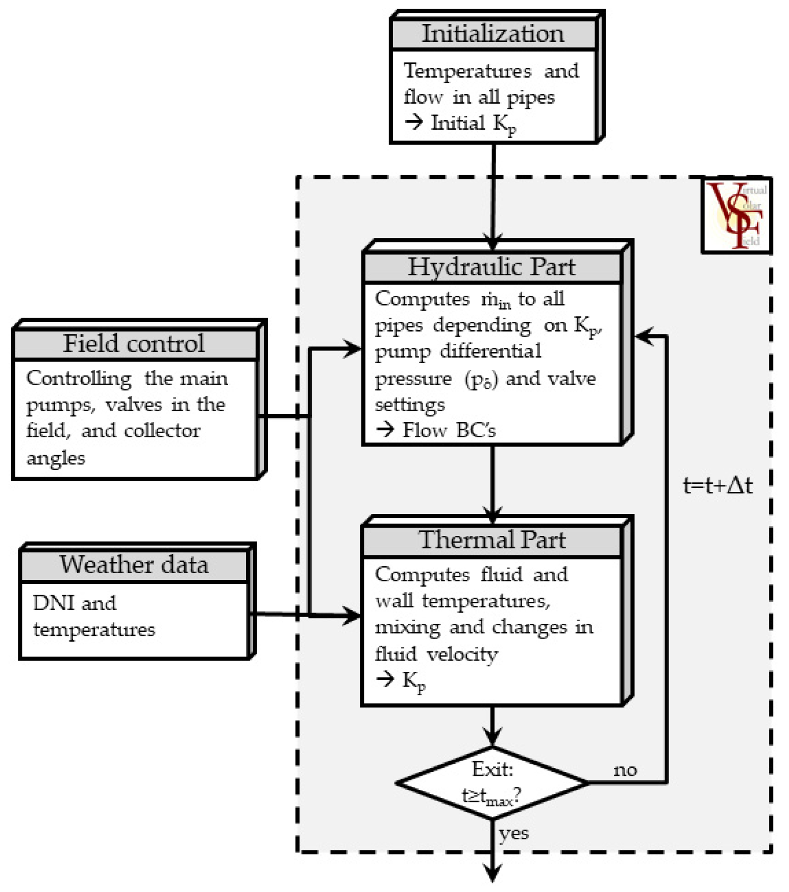
Figure 1 depicts the solution algorithm adopted in VSF, as well as, the components of the simulation tool. Firstly, the hydraulic solver computes the flow distribution depending on temperature-dependent and fluid-specific pressure losses in the different pipes and on the setting of the valves. This gives the flow boundary conditions (BC) to the thermal solver, which then, computes the temperatures based on one-dimensional discretization of the continuity and energy equations for the flow in all receiver pipes (loops), and header and runner pipes. A simplified model for the thermal losses in the receiver pipes is adopted by using empirical relations without modeling the glass envelop. Finally, the temperatures at pipe intersection nodes are computed by enthalpy balancing. The use of the hydraulic and thermal solvers results in adequate coupling of the thermal and flow conditions in the field without the need to solve discretized momentum balance equations for the fluid in the thermal part. This results in a computationally efficient algorithm to model whole solar fields having total piping lengths in the order of hundreds of kilometers in real-time for the intended applications. The model is thoroughly described in [
17,
20] including the model validation cases against commercial solar field data provided by Andasol-III.
The hydraulic part is based on methods described in [
21,
22] for solving large water networks and adapted to consider temperature dependent fluid properties of typical fluids in CSP plants including thermal oils and molten salt. The principle is based on mass flow balancing in the intersection nodes in a closed hydraulic network which ensures fluid continuity in the system. The energy balance for each closed loop within the network is described by the pressure form of the Bernoulli equation for viscous fluid flow, such that all pressure losses in the loop should sum up to zero, or to any external pressure source applied if there is a pump in the loop. The Newton-Raphson scheme is used to derive the set of linear equations system, which is solved by the linear algebra library, Armadillo [
23].
The main governing equations for the thermal part are the one-dimensional energy linear density equations for the fluid (subscript
f) and walls (subscript
w), which are given according to [
24,
25,
26] by
is the density, and
and
are the inner and cross-sectional area of the pipe, respectively.
is the specific heat capacity,
is the temperature, and
represents the coefficient of thermal conductivity. The one-dimension assumption is established in literature for this application as the radial temperature distribution does not have major consequences on the energy balance at the large scale and also during turbulent flow regimes. The wall energy source term,
can be expressed as
where
is the incident solar energy per unit length of the absorber tube as explained in
Section 2.1 and
represents the thermal energy losses per unit length from the receiver pipes. The convective heat transfer,
, is proportional to the temperature difference between the wall and fluid according to the coefficient,
, and convective specific surface area,
, such that
The coefficient
is computed using the Dittus-Boelter relation for forced convection heat transfer in turbulent flows. For low velocity flows with Reynolds numbers below
, free convection also becomes significant and is computed as a function of the Rayleigh number as in [
27].
The losses, , are computed using simplified empirical relations in terms of provided for common receiver manufacturers. The fluid mass continuity equation is also solved to consider fluid expansion and contraction as it is heated and cooled, respectively. As for the header pipes, heat transfer rates are much lower than in the absorber tubes due to the thick insulation material. Hence, a single header temperature is used to represent the fluid as a model simplification. This will affect the start-up time of the solar field where the header pipe temperatures are low as compared to the solar field inlet temperatures from the cold storage tank. However, this is not significant for the investigated test cases during normal operation of the solar field.
VSF also offers a high degree of flexibility in setting the geometry of the pipes, the number of loops and subfields, the type and quality of collectors and receivers, and the type of insulation material in the header and runner pipes. It is able to take any inhomogeneities of the plant design or manufacturing into account and consider the effect of such irregularities on the fluid distribution in the field. For example, a subfield might have different header lengths or diameters that would directly affect the flow rate going into it if not balanced by a throttling valve in the other subfields. Moreover, flow maldistribution can be modeled using this simulation tool. For example, to make the flow rate equal in all parallel loops in a subfield, throttling valves are used; however, partial shading of some loops can change the fluid properties due to cooling which causes flow maldistribution of the flow.
2.1. Solar Resource
In Equation (3), the absorbed solar energy,
, represents the energy input term to the system. As thoroughly discussed in [
28], the incident angle of the DNI with respect to a normal on a surface is represented by the solar altitude and azimuth angles. These angles depend on the times of the day and year, as well as the local latitude location of the surface. Different types of solar collectors have various solar tracking strategies that depend on the number of tracking axes, and the shape and orientation of the collector surface.
VSF considers parabolic trough collectors with single axis tracking oriented in the N-S direction. The effective solar irradiance falling on the collector,
, and the absorbed solar energy in the absorber tubes,
, can be expressed as
Firstly,
is the measured irradiance, DNI, falling per unit area of the collector and is multiplied by the net aperture width of the mirrors,
. It is corrected according to the sun elevation and azimuth angles by considering the cosine losses [
28,
29]. The incident angle modifier (IAM) is also multiplied by the DNI value to account for the efficiency loss in the collectors due to the off-normal incident sun rays. The IAM is computed for the SKAL-ET collector class according to [
30,
31].
Secondly, the combined optical efficiency is multiplied by the effective irradiance. The optical efficiency includes losses associated with the reflection of the mirrors, the absorptivity of the receiver tubes, the transmittance through the glass envelop, gaps between mirror panels and the intercept factor. The intercept factor includes errors in the mirrors, errors in positioning of the absorber pipes, sun-tracking errors, and the sun shape. Thirdly, the irradiation lost due to reflection beyond the absorber tubes and shading,
and
, respectively, are computed according to [
28] as a function of the sun incidence angle, the collector focal lengths and the spacing between the collectors. The shading factor is a value between 0 and 1 indicating how much of the incident solar radiation is not shadowed by the neighboring collectors. For N-S-oriented collectors, shading effects from collectors in the east and west directions are significant only at low sun angles during sunrise and sunset.
represents an efficiency factor due to the focusing of the collector in the sun direction, which depends on the deviation between the collector and sun angles.
2.2. DNI Maps and Nowcasting
With the presence of a detailed simulation tool that considers individual loops in a solar field, the spatial variation of the solar irradiance on the large extent of the field can be considered. Two distinct nowcasting system capable in deriving spatial DNI information for current and future conditions were developed by the DLR over the last few years. The first system is based on upward facing cloud cameras. These cameras are equipped with fisheye lenses taking images of the entire sky. The image processing is divided into distinct steps:
Clouds are segmented by means of 4-D clear sky library (CSL), accounting for different atmospheric conditions [
32].
Geolocation of the clouds is identified by a stereo photography block correlation approach with difference images. Detected clouds are modeled within a 3-D virtual modeling space [
33].
Cloud motion vectors are identified from three sequential image series by a block correlation approach with difference images from a single ASI [
33]
Future cloud positions are generated by displacing the cloud models inside a virtual modeling space [
34].
Cloud transmittance properties are measured only for a few clouds, which shade ground based DNI measurement stations. The remaining cloud objects receive transmittance estimations according to their height, results of a probability analysis with historical cloud height and transmittance measurements as well as recent transmittance measurements and their corresponding cloud height [
35].
Cloud shadows are projected to a topographical map with ray tracing [
34].
Shadow projections are combined with the ground-based irradiance measurements and the cloud transmittance properties to spatial DNI maps [
34].
The second approach is based on shadow cameras mounted on the top of a high building (e.g., solar tower) [
36] or on the top of a mountain range [
37] taking images of the ground. In this work, however, only cloud camera systems are used.
Achievable ranges and resolutions of the nowcasting systems depend on the used camera setups and configurations. The nowcasting system used in this work is operated at the Plataforma Solar d’Almería in southern Spain owned by the Spanish research center CIEMAT.
Table 1 lists the specifications of the used camera setup.
Satellite derived data produce much lower temporal and spatial resolutions which do not match the necessities of dynamic plant modeling, and hence, are not suitable for the application [
38].
The used DNI maps are spatially and temporally interpolated to provide input matrices to VSF, such that an effective irradiance value is given for each collector at each time step. The spatial interpolation process is done using the intrinsic MATLAB
® function interp2 which performs linear interpolation from the surrounding points in a two-dimensional mesh. The temporal interpolation depends on linear interpolation between the measurement points. More information can be found in [
39], where the processes are more thoroughly described.
3. Solar Field Controllers and Performance Assessment Scheme
Solar field control is an established topic in literature and in practice. Different aspects of common controllers in solar fields operating with single-phase HTF, commonly thermal oils, are discussed in [
25,
40,
41]. In reality, the implemented controllers fail to perform well during transient processes with high spatial variability like passing clouds especially. It has been reported that the solar field operators often prefer to manually operate the solar field during cloud passages to avoid excessive defocusing and to maximize the energy yield. Also, the operators need to intervene to stabilize the field outlet temperature during transient conditions to avoid thermally stressing the heat exchangers and other components in the power block.
In this section, an implementation of state-of-the-art solar field control is described. It is then adapted to be capable of automatically control the solar field and is used as a reference strategy. In
Section 3.2, an advanced controller that uses the nowcasting system is described. In order to quantify the benefit that an advanced controller can provide, the performance assessment scheme described in
Section 3.4 estimates the economic gain in comparison to the reference case.
3.1. Reference Controller
Numerous solar field control concepts are reported in literature, for example, common main flow controllers are described in [
25,
41]. Moreover, a simple PID controller is modeled and described in [
42]. More advanced control concepts which, to the knowledge of the authors, have not yet been implemented in large commercial projects, like model-predictive and fuzzy logic controllers are briefly outlined in [
43]. However, a lot of challenges regarding automatic solar field control have been reported due to the local variations in irradiation on the large solar fields. Thus, an automatic reference solar field controller has been developed and implemented, so that the VSF can run independently and be used to test new control concepts. The goal is to develop controllers that are robust to various realistic irradiation conditions. This has been introduced in [
44] and is briefly discussed in this section.
The main solar field flow controller alters the inlet mass flow to stabilize the solar field outlet temperature to a set-point at different weather conditions. The flow in VSF is controlled by the differential pressure,
, along the solar field which is sometimes referred to as pump pressure within the text. The pump is assumed to follow a first-order dynamic behavior with a time constant significantly faster than the system dynamics, typically 12 s [
45]. The pump pressure is also bound by minimum and maximum values that can be varied depending on the system design. The components of the control concept are described in detail below.
A feed-forward (FF) pump controller computes the required mass flow depending on the current total solar power incident on the field,
. This provides immediate response to global irradiance variations on the field. A simple plant performance model based on static energy balance in the whole field is used for the FF controller as described in [
25,
46,
47]. The required mass flow rate in the solar field to achieve a prescribed temperature rise in the solar field,
, is calculated as
is computed from average values of the available irradiance measurement points in the solar field. is the total thermal losses in all the header pipes and loops in the field computed in the VSF. is the average specific heat capacity integrated along the range of temperatures in the solar field.
To translate the required mass flow to a pressure drop along the hydraulic network, we use the hydraulic system curve. The system curves are produced by keeping a constant temperature in all the pipes and noting the total mass flow rate as the differential pressure is varied. The required pressure from the FF controller is thus computed as
with temperature-dependent coefficients,
and
, which are polynomial-fitted from different simulated data.
A temperature feedback PI-controller is added to provide closed-loop system control to account for the transient behavior of the field and for spatial variation in DNI. The controller corrects the pump pressure by a value,
, depending on the solar field outlet temperature feedback. A temperature set-point is given to the controller and the deviation from it,
, is computed. The change in pressure difference is given by the PI-controller as
The controller tuning parameters,
and
, are adaptively computed based on the first-order plus dead-time (FOPDT) method. They depend on the field load point, like solar energy input and losses, as well as the thermal inertia and fluid travel time in the pipes to compute the time constants and process dead times [
48]. This renders the controller suitable for a wide range of operation conditions as typical for the solar fields [
20]. The controller output is bounded to ±3.5 bar and, to avoid accumulation of the integral part of the controller as the output reaches the limit, an anti-reset windup (ARW) loop is added. The input to the ARW is the maximum allowable positive and negative changes to pump differential pressure,
and the PI-controller output is then bounded to these values.
Due to the fluid travel time in the long header pipes, which is typically around 10 min from the first loop to the power block, the temperature Feed-back (FB) controller provide delayed response. This often results in excessive defocussing especially during cloud passages. To emulate what a manual operator would normally do, a FB loop observing the focusing condition of the solar field has been added to the flow controller. It forces the controller to push in more fluid to reduce the temperatures in the SCAs, hence excessively defocused collectors back to tracking result. The control diagram is shown in
Figure 2 where all three control components are shown, namely, the flow FF loop, the temperature FB controller and, finally, the focus FB (FFB) loop. The FFB controller does not directly control the pump; it, rather, alters the temperature error,
, using a PI-controller that indicates over heating when higher flow rate is needed and also signals field cooling to reduce the flow rate causing more defocusing in the case when solar energy dumping is needed. Using this method, we avoid having an over-determined system, where more than one controller controls the same parameter, in this case the change in pump pressure,
. An ARW component is also added for this controller.
Finally, local PI-controllers in the SCAs regulate the collector temperatures assuming load-dependent set-points for typically 4 SCAs in series. The controllers manipulate the collector angle to adjust the defocussing ratio.
3.2. Advanced Control Using Nowcasting Data
Technologies using cloud and shadow cameras are able to provide highly spatially-resolved DNI maps with short-term forecasts. These maps not only serve as elaborate test cases for realistic irradiance to the VSF, they can also be used by the controller to improve the field operation and increase its energy yield.
As described in Equation (7), the mass flow FF controller uses the available DNI measurement points to estimate the required mass flow in the field according to the available solar resource. However, few measurement points, typically 2–5, are not sufficient to provide information about the current irradiance situation, especially during partial cloud coverage. The FB controllers do a good job to correct the effect of false input to the FF controller; however, their response is always delayed by the system dead-time and process time constants. This results in sub-optimal performance during transient conditions when the spatial variability of irradiance is high. Now, with the availability of irradiance maps, the spatial variability is available to the controllers and the response delays could be significantly reduced. For the advanced controller, the FF controller is slightly modified to act upon the average of the whole DNI map instead of only the average of the point measurements from weather stations.
3.3. Simulation Set-Up
VSF makes it possible to quantify the benefit of the nowcasting system on the field control in different situations. This contributes to investigating the feasibility of adding such systems, like cloud cameras, to a solar field and, by computing the expected revenues, it gives a good estimate of the return on investment.
To study this, we used DNI maps to compute the revenue increase for each of the days shown in
Figure 3 in comparison to the revenue from weather stations data. The weather station measurements are taken from single points on the irradiance map to provide consistent comparison and avoid effects of measurement errors from different equipment. The 25 test cases are chosen to include a wide range of DNI fluctuations as well as a variety of distinct cloud height combinations (including complex multi-layer conditions) and thus cloud types (see
Figure 3).
It is important to note that we assumed that DNI maps provide exact prediction of the irradiance falling on the collectors. This means the map values are treated as the real irradiance configuration. At the same time, it is assumed that the controller has access to exactly these data, thus considering a nowcasting system with no measurement errors.
3.4. Assessing Controller Performance
If the flow controller fails to provide the adequate flow rate in the solar field, the HTF will either overheat and cause defocusing of the SCAs, or will be cooled down resulting in a lower solar field outlet temperature. Both cases result in a reduction in the field performance and energy yield, which is challenging to quantify. In order to evaluate the performance of the different controllers, energetic penalties for collector defocusing and reduced field outlet temperatures have been developed. The penalties are calculated and summed up, such that the total penalty is
where
,
, and
are the penalties due to defocusing, and reduced power block and thermal energy storage (TES) efficiencies, respectively. The penalties are computed in monetary value in an effort to estimate the economic benefit or loss of using a specific control concept in specific situations. Then, we compute the penalties as percentages of the calculated revenue for the investigated time interval.
To make the economic computations more realistic, we performed an annual yield simulation of the investigated power plant configuration using Greenius simulation tool developed at the DLR [
49]. The simulation provides annual averages of the LCOE and power block conversion efficiency,
, which is estimated as
where
and
are the annual net electric energy output of the power plant and thermal energy input to the power block, respectively. Each kW
th of energy not collected due to defocusing results in an economic penalty of
is the solar energy lost due to defocus in the respective time interval, which is equal to the sum of lost solar energy in the collectors defined by . The value of is the amount of focusing of the SCAs as a function of time.
Another important factor that makes a good controller is the field outlet temperature. off-design field outlet temperatures reduce the power block efficiency, as well as that of the TES. In order to penalize a reduced PB efficiency, we estimate the performance at the design temperature,
, using a detailed heat flow diagram of the PB implemented in EBSILON
® Professional. From this model,
, is derived as a function of the HTF temperature as shown in
Figure 4 for a 50 MW turbine assuming the temperature correction is independent of PB load. Thus, the reduction in HTF temperature is penalized as
Finally, we add a penalty to account for the reduced stored energy due to low storage medium temperatures being pumped in the hot tank with limited capacity. As the tank gets full, any thermal energy more than the PB capacity is an overload and will need to be dumped. The penalty value of such instances of dumping due to reduced storage efficiency is calculated as
T and
Tin are the field outlet and inlet temperatures, respectively,
T0 is the design field outlet temperature. The factor,
represents the loss in stored thermal energy due to the reduced temperature. The ratio
is the annually averaged ratio of TES overload resulting in solar energy dumping in the SF, which represents how frequent the TES is overloaded on a yearly average. Both annual averages are estimated from the Greenius simulations. The simulation results for the La Africana power plant set-up with yearly irradiance data are listed in
Table 2.
The absolute penalty values have not been validated against real power plant data. However, they serve as reference values when comparing different control concepts and give an order of magnitude of the economics. To provide a normalization value, the theoretical revenue is computed. This corresponds to the expected revenue from an ideal controller, which is able to maintain the field outlet temperature at the set-point without any control-induced defocusing, and neglecting heat losses in the solar field. The theoretical revenue is computed as
On the other hand, the actual revenue results from transforming the thermal energy output of the field into electrical energy and is computed as
The penalties due to defocusing are already included in RSF, hence, only the additional penalties due to the reduced field outlet temperatures are subtracted. Other losses in the field correspond to the thermal losses and are computed as
Thermal losses depend on the fluid temperature of the field, as well as the flow rate and are, hence, influenced by the field operation and control. In
Table 3, the revenues and penalties for different control concepts in various DNI conditions are compared to provide a comprehensive and reliable measure of the plant and controller performance.
4. Results
In this section, some results of applying the control concept described above are shown. The commercial power plant La Africana near Posadas in the province of Córdoba in Spain [
50] is simulated and used as a test case. The plant geometry and layout are provided by the plant operators, Africana Energía, through a collaboration with industrial partners including TSK Flagsol Engineering GmbH. La Africana is designed to provide 50 MW of electric power. Its solar collector field has 4 subfields with a total of 168 loops and DOWTHERM
® [
51] thermal oil is used as the HTF. For all the simulations performed in this study, a constant solar field inlet temperature of 290 °C is used. The plant has two molten salt (MS) tanks that are used for thermal energy storage; however, they, as well as the power block, are not simulated within this entire work. La Africana is equipped with two weather stations located in the NE and SW corners in the plant as indicated in
Figure 5.
DNI maps provided through processing cloud camera images are used as the input energy source to the simulated solar field. The maps provided from PSA have a temporal resolution of 30 s and a spatial resolution of 5 m × 5 m and cover a total area of approx. 2 × 2 km. The irradiation values are interpolated to the single SCAs to establish a spatial distribution of the energy input to the field. A reference control concept is modeled as explained in
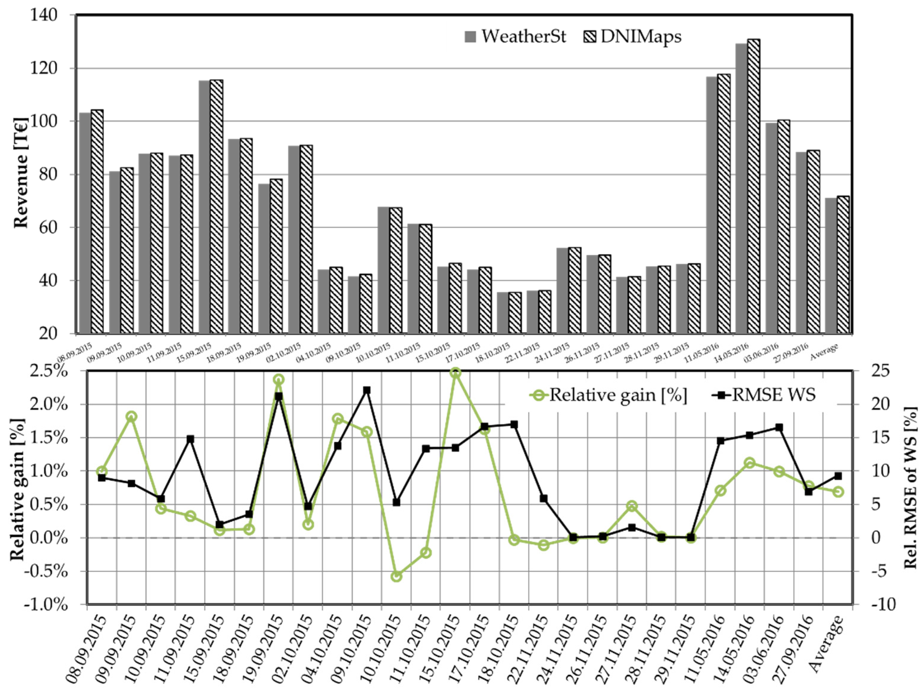
Section 3, such that the input solar irradiance value to the feed-forward part of the controller is the average of two-point measurements extracted from the DNI map. These two points emulate the measurements achievable by the installed weather stations in La Africana. The performance is then compared to the performance of an advanced solar field controller that uses the average value of the whole DNI map falling on the SCAs as input instead. The average, maximum and minimum effective irradiance extracted from a DNI map for an exemplary day are plotted in
Figure 6. Solar field start-up is not considered in any of the investigated cases.
In total, 30 representative days as explained in [
32] were investigated within this study. However, five days with too low DNI levels and high data scattering were excluded from further analysis. Those days do not represent typical solar field operation days and an operator would most likely not be able to maintain stable energy output from the field. For the remaining 25 days, the expected revenues are compared in
Figure 7 for the cases using weather stations and DNI maps. The revenues are normalized by the maximum theoretical revenue possible giving a relative revenue gain. The relative revenue gained from using the nowcasting system is computed for each day as
This is represented by the green line on the left vertical axis. The root-mean-square error (RMSE) between the average
computed from the two weather stations and that from the maps for each test case is computed as
It is then normalized by the average irradiance of the maps to provide comparable values for the various cases and shown by the black line on the right axis. The normalized root-mean-square error (nRMSE) indicates how inaccurate the average of the measurement of the weather stations is as compared to the actual average DNI on the field. The mean values for all 25 days are also plotted in the figures. On average, the nowcasting system improves the yield by 0.69% making approximately €493 per day of operation. The maximum relative gain is approximately 2.5% on 15.10.15, while the maximum absolute revenue gain per day is round €1820 on 19.09.15. The advanced controller, however, causes a slight drop in the performance during 3 days showing the worst performance of −0.57% and −0.22% on 10.10.15 and 11.10.15, respectively. For clear-sky days like on 24.11.15 and 29.11.15, the nowcasting system does not show any benefit, since there is no spatial variability in DNI and the measurements of the two weather stations are sufficient to represent the real situation. All results are summarized in
Table 3 and graphically in
Figure 7.
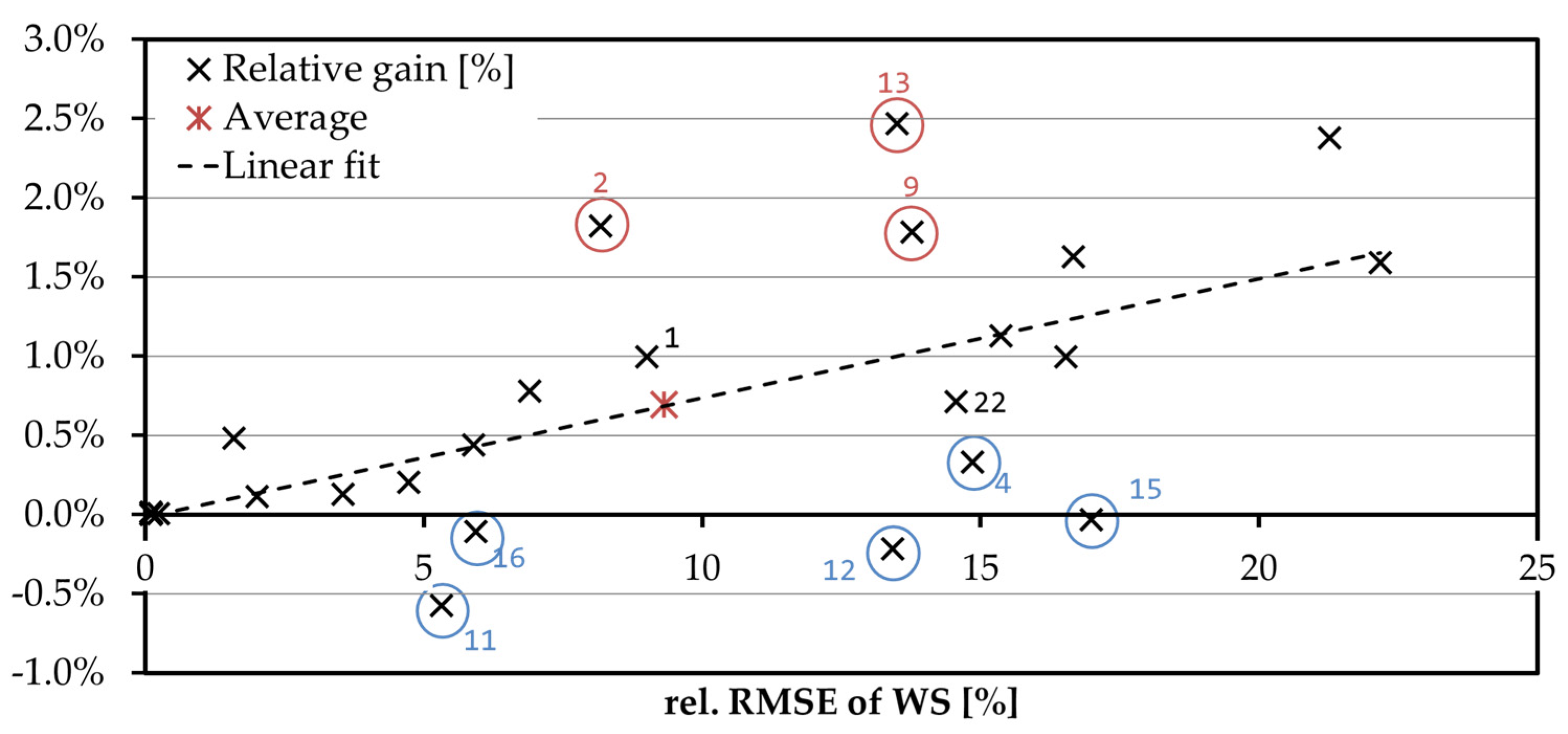
The trend of the revenue gain (green line) follows the trend of the nRMSE of the average value of the two weather station measurements. In
Figure 8 the relation is more clearly observable, where a linear trend can be fitted to the data. In general, the more the measurements deviate from the real situation, the more benefit is gained by using the nowcasting systems. The clear outliers are marked by circles on the figure. The red circles represent the days showing exceptionally higher revenue gains, while the blue ones represent the days with low revenues gains or even some deficit.
The trend of the revenue gain (green line) follows the trend of the nRMSE of the average value of the two weather station measurements. In
Figure 8, the relation is more clearly observable, where a linear trend can be fitted to the data. In general, the more the measurements deviate from the real situation, the more benefit is gained by using the nowcasting systems. The clear outliers are marked by circles on the figure. The red circles represent the days showing exceptionally higher revenue gains, while the blue ones represent the days with low revenues gains or even some deficit.
By having a closer look at the outliers, the following can be observed. For the red outliers labeled by cases 2, 9, and 13, the relative revenue gains are exceptionally higher as compared to other days having similar nRMSE. For example, case 2 has a revenue gain of approximately 1.82% and an nRMSE of 8.17% in contrast to case 1 in its vicinity, which shows a gain of only 1% and an nRMSE of 9%, which follows the linear fit. This shows that the potential benefit of the nowcasting system depends on the specifics of the variations in DNI, like intensity and frequency of the spatial and temporal fluctuations. This needs to be further investigated and is not part of the study presented in this paper. Another observation is that the system provides more revenue gain on days with lower DNI levels as compared to other days showing similar spatial variability. For example, case 9 has a theoretical revenue of approximately €58,000 while case 22 has a theoretical revenue of approximately €130,000. Lower DNI levels result in lower overall mass flow and higher thermal losses relative to the thermal energy input, which empathizes any improvement in performance.
On the other hand, the advanced controller resulted in revenue losses as compared to the reference controller for the cases 11, 12, and 16. A significantly less revenue gain is observed for cases 4 and 15. For all five cases the drop in revenue in the advanced controller is a result of switching more readily to the antifreeze mode causing all SCAs to defocus and lose solar thermal energy.
Figure 9 shows 2 exemplary instances where the advanced controller goes into antifreeze mode since the average
of the whole map drops below the threshold of 130 Wm
−2. On the other hand, the reference controller will stay in normal operation mode. The effect is prominent in cases 11 and 16 since these days are dominated by clear-sky or uniform shadows except for the few instances described as shown in
Figure 10. When we reduce the threshold to 100 Wm
−2, the loss is significantly reduced to −0.03%; however, this allows the flow to be too low, such that overheating and extreme temperature gradients can take place when the sky is clear again.
Figure 11 shows the
in case 4. The day is dominated by high spatial and temporal fluctuations and it should be expected that the advanced controller would follow the linear trend in
Figure 8. The trend is perfectly followed until 9 h after the start. In the last 2 h, the same irradiance conditions as in cases 11 and 16 take place which causes the slight drop in the revenue gain. The same behavior is also observed for case 12.
Although absolute revenue values strongly depend on the accuracy of the annual yield simulation results listed in
Table 2, the comparison between the revenues in both cases indicates the expected order of magnitude for the benefit of using the nowcasting systems. Assuming that the investigated 25 days are representative for 300 days of operation of the solar field, we could estimate the extra revenues from installing the nowcasting system to be in the order of €100,000 to €150,000 per year. Provided that the system produces sufficiently accurate DNI maps, it is expected to cover the investment and operation costs in less than a year making the system economically feasible.
5. Conclusions and Outlook
As more CSP projects are being built, continuous advancement and improvement to the field controllers is necessary. Moreover, new developments in related research and application fields, such as meteorology and control hardware, render it possible to incorporate more sophisticated control concepts and foster the energy yield of solar fields. In this paper, an evaluation process for novel technologies based on a detailed simulation model for parabolic trough solar fields is presented. A reference case is defined and programmed within the simulation tool, the virtual solar field (VSF). Then, the advanced concept is incorporated and the performance is assessed and compared with the reference case. Consequently, the economic impact can be estimated to predict the feasibility of the technological advancement without interfering with plant operation and at less cost than building test benches.
To demonstrate this, a reference automatic flow controller is developed to represent a state-of-the-art solar field. This allows testing the potential benefits of using spatially resolved DNI maps for the field control instead of relying on two weather stations measurements only. Nowcasting systems using a set of upward-facing cloud cameras provide the DNI maps for the solar field area. Then, a novel controller employs the maps with more precise information about the average incident irradiance on the solar field to improve the plant performance. This overcomes the limitation of using local measurements of only a few points, where most of the information about the spatial variation is lost. It also helps the controller to provide more adequate flow to the field and avoid defocusing instances and excessive temperature drop during cloud passages. The performance of the solar field is simulated using VSF and an estimation of the expected revenues is computed according to the controller assessment scheme described in
Section 3.4. A total of 25 days are investigated and the average increase in revenue is found to be 0.69% translating to an estimation of €100,000 to €150,000 of surplus in income per year. In addition, using the average of a whole map smears out abrupt changes in irradiance and reduces the intensity of fluctuations in the feed-forward controller.
It is important to note that these results are obtained assuming perfectly accurate prediction of the DNI maps. Studies in [
20,
44] show that the controllers are robust to systematic errors in irradiation measurements of up to 10% without significant loss in revenues. However, stochastic errors are expected to have an impact on the benefit of the system. Initial studies show a slight impact on the revenues while still guaranteeing a significant benefit of the system. More investigations of the effects of uncertainties in the maps are currently being performed.
On the other hand, higher potential can be achieved by the system if the controller could automatically identify the conditions, where the nowcasting system causes revenue losses as shown in a few cases. This can be predicted using only current DNI situation or using the short-term forecasts provided by the system. Then, for these cases, it uses only the data provided by the weather stations. This would result in an annual increase of approximately €20,000 in revenues by only avoiding additional losses.
This paper also triggers the need to provide adequate controller parameters designed specifically for the incident irradiance condition. This requires the classification of the DNI situation according to the spatial and temporal variability on the solar field. A study shows that such classification method has a potential to improve the yield by a further 1–2% with respect to the reference controller [
52].
Moreover, advancements in cloud detection and motion prediction can provide accurate irradiation maps and even short-term forecasts paving the way for optimized solar field control with model-predictive approaches. Also, the economic and technological feasibility of solenoid control valves and improvement in network communications offer the possibility to control the flow in each single loop to account for any local transients with very high resolution.
Nevertheless, the economic benefit of applying such advancements is yet to be proven. The process presented helps to estimate the benefits and feasibility before applying the control strategies to real solar fields, which reduces the commissioning time and risks, and avoids interrupting the operation of the power plant.


