1. Introduction
Buildings are rated among the most energy-intensive uses, consuming approximately 40% of the worldwide energy demand, with CO
2 emissions of up to 36% [
1]. In this context, buildings have seen the progressive evolution of energy systems due to a consistent introduction of renewable energy sources and storage systems, also thanks to incentive programmes (such as
“20-20-20”) [
2] conceived of to support the reduction of energy waste through the implementation of optimal control and energy management strategies. Building energy management has become a complex process, considering that modern energy systems have to respond to on-site intermittent renewable sources, energy storage, grid requirements and electric vehicle charging, in addition to traditional services such as lighting, ventilation, and air conditioning [
3].
HVAC often represents the most energy-intensive building use [
4], especially in the non-residential sector, although significant improvements have been implemented in recent years to enhance their energy efficiency.
One of the main challenges related to the optimal management of HVAC systems consists in handling the nonlinearity of the control problem given the effect of several stochastic endogenous (e.g., occupant behaviour) and exogenous (e.g., weather conditions) factors. Therefore, researchers have focused their attention on innovative control strategies for HVAC systems, capable of maintaining indoor thermal comfort conditions and, at the same time, reducing their energy consumption. Eventually, these strategies need to be also able to handle signals from the electrical grid in order to meet power requirements and improve the grid reliability and stability [
3,
5].
These opportunities were provided by the introduction of Automated System Optimisation (ASO) tools based on artificial intelligence (AI), which can contribute to significantly enhancing the energy flexibility of a building. The energy flexibility represents a fundamental characteristic of smart buildings that defines their ability to adapt and respond to grid requirements, climatic conditions and user needs [
6,
7].
Traditional controllers, such as ON/OFF or Proportional-Integrative-Derivative Control (PID), could be inadequate due to their inability in foreseeing the dynamic changes that impact the operation of energy systems [
8].
The ON/OFF control regulates a process operating within boundaries, while the PID requires the tuning of the control parameters prior to its deployment [
6]. Although the latter has better performance than ON/OFF controllers, it could still be inadequate because the performance of the PID decreases significantly when the operating conditions are different from the tuning conditions in which the constants that regulate the control are calibrated [
9]. Today, PIDs are the most common bottom-level control systems, while rule-based control systems (RBC) are considered the standard for optimising the management and top-level control of HVAC systems, but the resulting energy savings are limited [
10,
11]. In fact, RBC strategies are fixed and not scalable to different climatic conditions or building features as well as unable to predict changes in HVAC systems [
3].
To overcome such limitations, the application of model-based control strategies has been explored in the last few years. In particular, Model Predicted Control (MPC), has become a dominant control strategy in research on intelligent building operation [
12]. However, despite the implementation of MPC has shown its excellent ability of improving thermal comfort and reducing energy consumption between 15 and 50% [
13,
14,
15], in both simulative [
16] and real test environments [
17], its model-based nature represents in some cases a critical aspect.
In fact, a significant problem in MPC is related to the performance dependency on the model definition for the control strategy optimisation, which is often challenging to design with good accuracy. Moreover, it is challenging to generalise its use on different types of plants and buildings. As a result, MPC controllers have not been adopted as expected in the building industry despite the promising results [
18].
As a consequence, research has also focused on the development of model-free controllers based on Machine Learning (ML), which has shown great potential for improving the performance of buildings [
19], particularly when Reinforcement Learning (RL)-based algorithms [
20] are implemented. The interest in control strategies based on RL has increased since it does not require prior knowledge of the process or environment to be controlled.
A control agent based on Reinforcement Learning algorithms learns an optimal control policy by the direct interaction with the environment through a reward mechanism which depends on the control action performed in a specific state of the controlled environment [
21]. Due to its simplicity, Q-Learning is the most commonly used technique in the Reinforcement Learning field [
22,
23]. However, in some circumstances, this algorithm proves to be not optimal when implemented in building control systems that require the definition of a high number of states and actions and greater complexity in the exploration of nonlinear relationships for the controlled environment. To overcome this obstacle, deep neural networks have been employed to approximate the policy function, as in Deep Reinforcement Learning (DRL).
In the next section, reference studies about the use of the DRL control strategies in HVAC systems control are reviewed, along with the motivations and the novelty of the present contribution.
Related Works, Motivations and Novelty of the Paper
The interest in Reinforcement Learning for the control of energy systems has grown in recent years, even if its applications still remain limited.
The first RL application in the energy and building research field dates back to 1998, in which [
24] RL was used on an HVAC system serving the DOE (Department of Energy) at Idaho State University, to control the water temperature leaving boiler and the temperature in the two thermal zones served by the system. The applications of DRL for the control of HVAC systems have increased considerably, with the aim of regulating different parameters such as: supply water temperature setpoint [
5,
25,
26], storage tank temperature setpoint [
27,
28,
29] supply air-flow rate [
30], supply air temperature [
31], indoor temperature setpoint [
29,
32,
33,
34], frequency of pumps and fans [
35,
36]. Zhang et al. [
5] applied a DRL control type Asynchronous Advantage Actor-Critic (A3C) in a water-based Radiant Heating System, in which the hot water pipes were integrated into window mullions with the objective of reducing the energy consumption of the system while ensuring the internal comfort of the occupants. The adaptive control system operated on the supply water temperature setpoint of the radiant heating system and was able to reduce energy consumption by 16.7% with a slight increase in the Percentage of Person Dissatisfied (PPD).
A further application of DRL control strategies on radiant heating systems was recently proposed by Brandi et al. [
26], in which an algorithm based on Deep Q-Network was used to control the supply water temperature of the boiler in an office building. In that case, both static and dynamic deployment of the DRL controller were tested, and the heating energy saving in relation to a climatic rule-based control logic ranged between 5 and 12%, with enhanced indoor temperature control with both types of deployment. Moreover, that study highlighted the significance of an initial application of this control system into a simulated environment: the direct real-implementation would cause a reduction in the control performance since a DRL agent takes a long time to converge towards an acceptable control policy [
26,
28,
37]. Therefore, in most cases reported in the literature, an initial simulation phase is performed in which various tools are combined, such as EnergyPlus [
38] or CitySim with deep learning libraries such as Tensorflow [
39].
In other studies, Vázquez-Canteli et al. [
27,
28] applied an algorithm based on Deep Q-Learning to control a heat pump coupled with a cold water storage to minimise its electrical energy consumption achieving 10% of energy saving while maintaining adequate indoor temperature conditions compared to a Rule-Based Control (RBC). Yoon et al. [
30] proposed a performance-based thermal comfort control using Double Deep Q-Network to study the existing trade-off between building energy efficiency and improved comfort conditions for the occupants. Keeping the PMV value within the comfort range [
40,
41,
42], the proposed control strategy made it possible to reduce the VRF energy consumption by 32% and the humidifier system energy consumption by 12% when compared to a fixed RBC.
Some published works have been related to the application of DRL on occupant centric control problems in the built environment. In this context, Park and Nagy [
32] presented HVACLearn, a Reinforcement Learning (RL)-based Occupant-Centric Controller (OCC) for dynamically setting the thermostat setpoint, in which the indoor temperature, occupant behaviour and thermal vote were monitored to satisfy occupant comfort needs and enhance energy efficiency. The authors assumed that occupants could express their thermal sensation in real time by pressing two buttons of a sensing unit: too cold or too hot; an increase in the number of buttons pressed indicated a worsening of the indoor temperature-related comfort conditions. The authors simulated HVAC Learn control in a single occupant office with occupant behaviour models and, compared to an RBC, obtained a significant reduction of hot sensation feedbacks from the occupants while consuming the same or less cooling energy.
This literature review proves that Deep Reinforcement Learning represents a great opportunity for the future control systems of HVAC systems, being in most cases more efficient than current widespread control systems in terms of improving energy efficiency and comfort conditions in buildings.
However, the majority of papers in the literature consider the deployment of the DRL agent after its offline pre-training, making this control strategy similar to that based on a model, since the effort required in the pre-training phase indirectly led to the definition of an offline model. The online training of the controller, instead, which would preserve the free-model nature of the RL simulating its direct implementation in a real context, was poorly explored in literature. For this purpose, in this paper, the online training of the DRL controller is performed on a simulation environment combining EnergyPlus and Python for an office building. In this way, it is possible to simulate the initialisation of the controller as it was implemented in a real building. In this case, the learning process of the agent consists of control strategy optimisation on the basis of the information retrieved in real time from the controlled environment.
Moreover, some issues related to the application of off-policy algorithms and the possibility of implementing a model-free algorithm in real world context arise from the literature.
In the case of on-policy algorithms, the agent tries to evaluate and improve the same policy used for action-selection. However, the controller does not explore other control policies than the optimal one learned during exploration, which may result in reaching a local optimum. Thus, an off-policy algorithm would allow the agent to continuously explore other policies for extracting action sets useful for optimising the current policy. This parallel learning process speeds up the learning process, reducing the time required for the control policy to converge to the optimum.
Therefore, in this paper, an off-policy algorithm named Soft Actor-Critic is implemented [
43]. This algorithm ensures the continuous agent exploration of new policies, but at the same time prevents the possibility that it transposes lousy trajectories. Another benefit provided by the Soft Actor-Critic algorithm is represented by the opportunity to choose actions in a continuous range, which is advantageous in the control problem of energy systems.
In this paper, an online implementation of a DRL controller is designed to enhance the indoor temperature conditions while reducing the energy consumption related to the heating system. This agent is designed to ensure the maximisation of the objective function through the control of the supply water temperature to the heating terminal units of a thermal office zone.
A sensitivity analysis is carried out on the hyperparameters of the model to assess their impact on the performance achieved by the control agent during its online training. Among all the DRL controller configurations, the one that ensured the best performance against a climatic rule-based control baseline is selected to perform a scenario analysis. The best configuration is adopted for testing the adaptive skills of the control agent by changing some forcing variables, consisting of eight different control scenarios. The adaptive performance of the agent is investigated following two deployment approaches, dynamic and static, in which the control agent is able or not, respectively, to update the control policy when changes are introduced in the environment.
Based on the literature review on DRL control logic in HVAC systems, the novelties that are introduced in this study can be summarised as follows:
A DRL agent is developed using the SAC algorithm for controlling the supply water temperature in a heating system operating in a real building. To the best of the authors’ knowledge, the SAC algorithm has been poorly explored, although it is recommended for controlling energy systems prone to dynamic changes in environmental conditions, such as HVAC systems. The SAC controller performance is compared with a rule-based climatic logic, to enhance the indoor temperature conditions and the energy efficiency of the system.
The control agent, different from most of the papers reported in the literature, is trained online using a calibrated energy model of a real building, using an integrated environment coupling EnergyPlus and Python. In this way, the performances of the agent can be analysed, as it is implemented in a real building without offline pre-training.
A sensitivity analysis on the hyperparameters is performed during the online training, in order to choose the agent employing the combination of hyperparameters that provides the best performance compared to the RBC baseline.
The adaptability of the DRL agent deployed online was tested for several different scenarios, including changes of outdoor weather conditions, indoor temperature requirements, occupancy schedules and internal heat capacity, for two different deployment approach, dynamic and static.
The rest of the paper is organised as follows. In
Section 2, the theoretical aspects of RL and the algorithms are provided. In
Section 3, the case study is introduced, while the implemented methodological framework is described in
Section 4.
Section 5 provides information about the simulation environment, the definition of the baseline controller and the design of the proposed DRL control logic. Moreover,
Section 5 also provides details on the deployment and scenario analysis. The results are presented in
Section 6 and discussed in
Section 7.
Section 8 includes the conclusions and includes future research directions.
2. Reinforcement Learning Overview
In the Reinforcement Learning framework, a control agent learns the optimal control policy through a direct interaction with the environment through a trial-and-error approach. RL can be formalised as a Markov Decision Process (MDP) that is defined by a four-values tuple, including: state, action, transition probabilities and reward. The state is a set of variables whose values provide a representation of the controlled environment. The action is the control signal that the agent performs on the control environment in order to maximise its goals encoded in the reward function. The transition probabilities define the probability of the environment to move from a state
s to a state
s′ when an action
a is performed. According to MDP theory, these probabilities depend only on the value of state
s and not on the previous states of the environment [
44].
The RL framework applied to a control problem in the energy management domain can be simplified as follows: a control agent (e.g., a control module linked to the building management system) interact with an environment (e.g., a thermal building zone). At each time step, the agent performs an action (e.g., setting of the supply water heating temperature) when the environment is in a certain state (e.g., the building is occupied, but the temperature is above the upper comfort band limit). The agent receives, along with the observation of the state, a reward that measures the performance of the agent with respect to its control objectives. Starting from a certain state of the environment the RL algorithm tries to identify the optimal control policy π that maximises the cumulative sum of future rewards. The optimal policy is determined by the RL agent by evaluating two functions, namely state-value function, and action-value function.
The state-value function represents the goodness of being in a certain state
St with respect to the control objectives [
45]. This function provides the expected value of the cumulative sum of future rewards that the control agent would obtain by starting from state
St and following the policy
π and it is defined as follows:
where
γ [0,1] is the discount factor for future rewards. For
γ = 0 the agent will give greater importance to immediate rewards. Conversely, for
γ = 1 the agent will seek to maximise only future rewards.
Similarly, the action-value function represents the goodness of taking a certain action
At in a certain state
St following a specific control policy
π [
46]. The action value function can be expressed as follows:
In the context of RL algorithms the most widely applied approach is the Q-Learning. Q-Learning exploits a tabular approach to map the relationships between states and action pairs [
25]. These relationships are formalised as state-action values or Q-values, which are gradually updated by the control agent through the
Bellman equation [
47]:
where
μ [0,1] is the learning rate which determines how rapidly new knowledge overrides old knowledge. With
μ = 1 new knowledge completely overrides what was previously learned by the control agent.
2.1. Deep Reinforcement Learning
Despite its effectiveness, Q-Learning may have inadequate results when the dimensions of the state and action spaces grows [
24]. To overcome this limitation, Artificial Neural Networks (ANNs) [
45,
48] were recently introduced to substitute lookup tables in mapping the relationships between states and actions in order to determine the optimal control policy. One of the main advantages of ANNs is their capability to handle continuous inputs and outputs making them suitable for a variety of control problems [
26]. Moreover, they have proven to be effective methods to capture hidden and nonlinear pattern among data [
49,
50]. RL algorithms which employ ANNs, and in particular Deep Neural Networks (DNN), are identified as Deep Reinforcement Learning (DRL) [
51].
2.2. Soft Actor-Critic
In this work a particular DRL control algorithm, namely Soft Actor-Critic (SAC), was implemented. SAC is an off-policy algorithm based on the maximum entropy RL framework, introduced by Haarnoja et al. [
43]. Different from Q-learning, SAC is capable of handling continuous action spaces, enhancing its applicability to a variety of control problems. Soft Actor-Critic uses a particular Actor-Critic architecture that employs two different deep neural networks for approximating action-value function and state-value function. The
Actor maps the current state based on the action it estimates to be optimal, while the
Critic evaluates the action by calculating the value function.
The main feature of SAC is the entropy regularisation: this algorithm is based on the maximum entropy reinforcement learning framework, in which the objective is to maximise both expected reward and entropy [
52] as follows:
where
H is the Shannon entropy term, which expresses the attitude of the agent in taking random actions, and
α is a regularisation coefficient that indicates the importance of the entropy term over the reward. Generally,
α is zero when considering conventional reinforcement learning algorithms.
The maximisation of this target function has a close connection with the exploration-exploitation trade-off, ensuring that the agent is explicitly pushed towards the exploration of new policies and at the same time avoids that it gets stuck in sub-optimal behaviour.
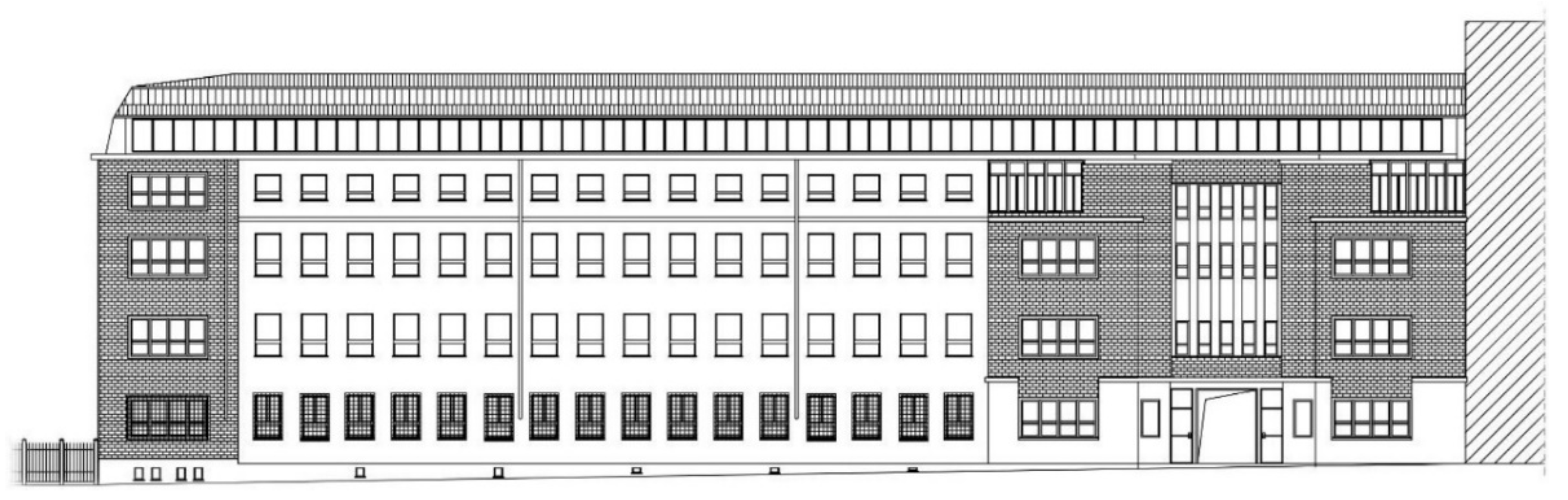
3. Case Study
The building investigated is an office building located in Turin, Italy, and consists of five heated floors and a basement, with a net heated surface of about 9300 m
2 (
Figure 1). The five heated floors are organised into two heating zones: the ground floor, and the remaining four floors.
The average transmittance values of the opaque and transparent envelope components are 1.08 and 2.7 W/m2K, respectively. The occupancy schedules were defined on the basis of the actual office opening and closing times. Every weekday, with the exception of Sundays and holidays, the office is occupied from 7 a.m. to 7 p.m.
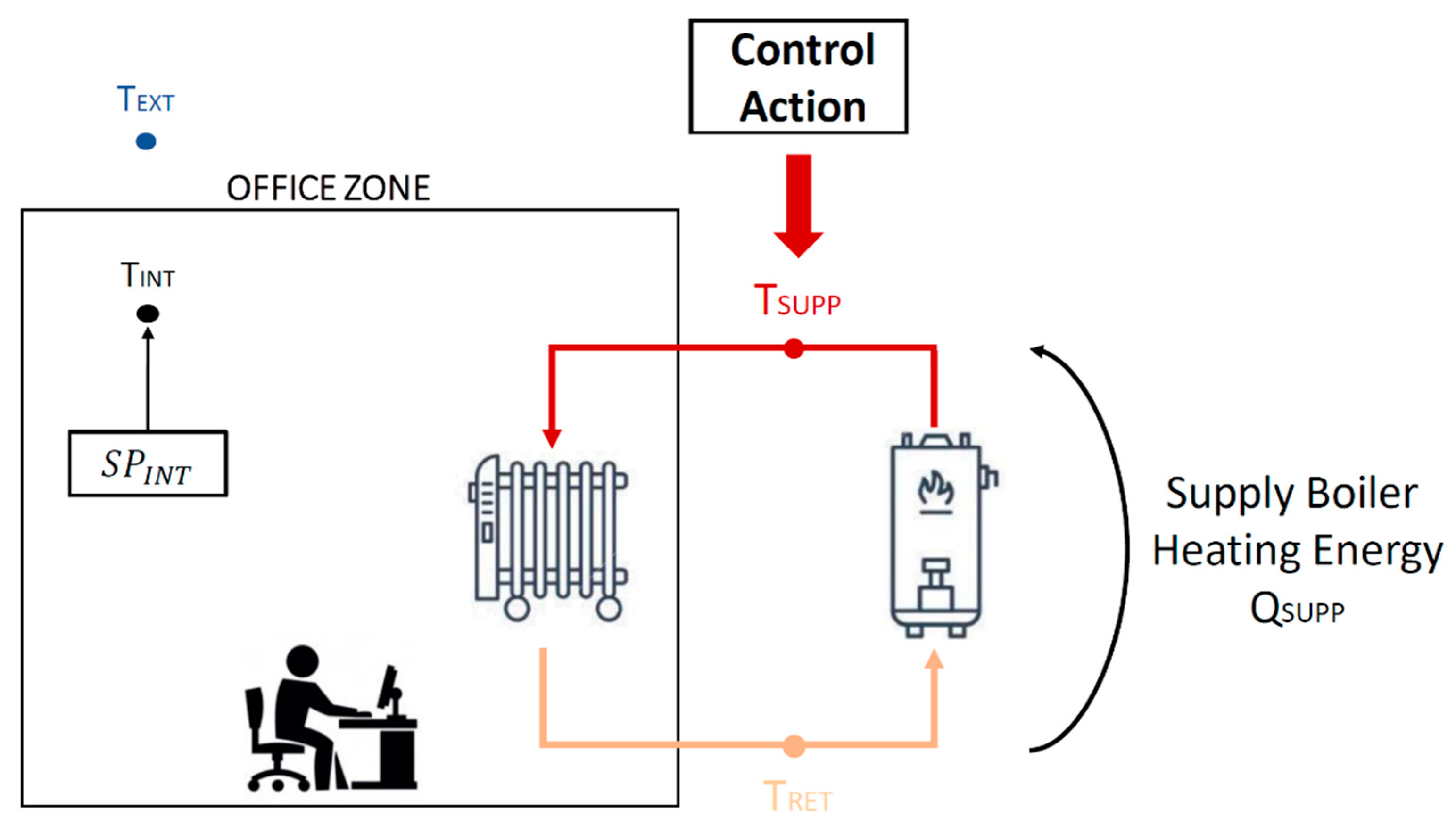
The two thermal zones are served by a hot water circuit consisting of two loops connected by a heat exchanger. Four gas-fired boilers (with a total nominal capacity of 1300 kW) are installed in the primary loop, serving a collector from which different pumps withdraw water to serve the radiator terminals in the secondary loop.
The supply water temperature is regulated in the installed control strategy through a constant speed pumping system and a three-way valve. The heating system implemented in the EnergyPlus simulation model consists of two different circuits serving each thermal zone with a gas-fired boiler that supplies hot water to the radiators for each circuit (
Figure 2).
This study was focused only on the indoor air temperature control, since the building is served by water terminal units, able to operate only on the sensible part of thermal load.
The energy model was calibrated through an iterative approach, using hourly indoor temperature and monthly boiler gas consumption data available for the real building. Thermo-physical properties were extracted from an energy diagnosis report that was available for the building under analysis. A manual calibration based on an iterative approach was performed, varying the infiltration airflow rate, internal gains and equipment power according to [
53]. However, considering the available information, the model was not calibrated from an indoor comfort point of view. This could lead to discrepancies regarding the real values of the calibrated variables [
54].
In this context, two statistical indices (MBE and Cv(RMSE)) were calculated, as suggested by the ASHRAE guidelines [
55], in order to prove the accuracy of the calibration process. The results obtained after the calibration process are reported in
Table 1.
The objective of the developed DRL controller is to maintain the desired temperature conditions during occupancy while consuming the minimum heating energy as possible, through the regulation of the supply water temperature to heating terminal units of the office zone. The controller is penalised if the indoor air temperature falls outside the temperature acceptability range, defined between [−1, 1] °C from the desired indoor temperature value of 21 °C. The same acceptability range 21 ± 1 °C was considered for the baseline controller.
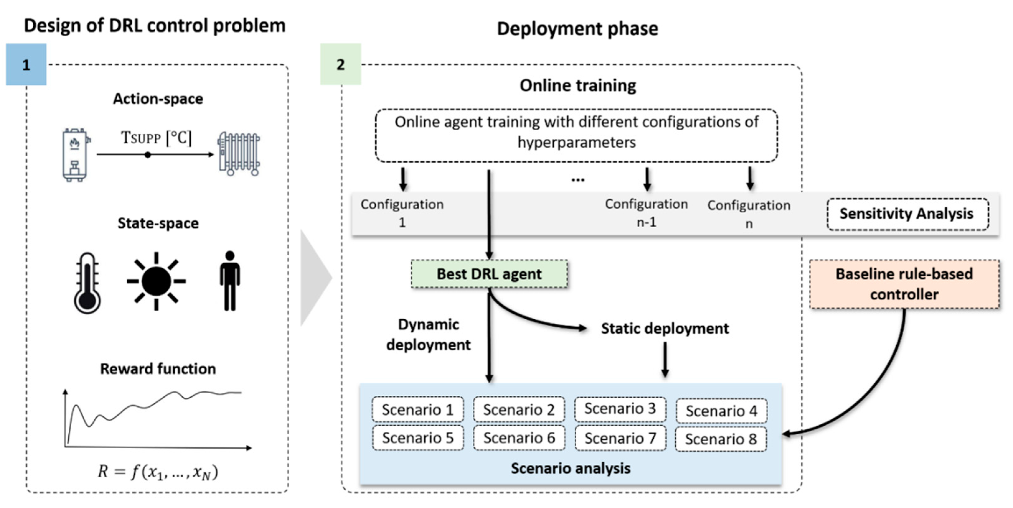
4. Methodological Framework
The methodological framework adopted in this paper unfolds over two different stages, as shown in
Figure 3:
4.1. Design of the DRL Control Problem
Initially, the main components of adaptive control logic were defined, i.e., action-space, state-space and reward function. The control actions to be selected by the controller were included in the action-space. The state-space includes observations concerning the state of the controlled environment for each control time step. This information is provided to the agent to learn the optimal control policy that maximise the objective function of the problem. The design stage was concluded through the definition of the reward function. This feature was defined accordingly with the target established for the agent.
4.2. Deployment Phase
After defining the action-space, the state-space and the reward function, the implementation of the DRL agent was investigated. The deployment framework consisted of two phases: the online training of the DRL agent and a scenario analysis. In both cases each simulation involved a three-month heating season, from 1st December to 28th February, repeated only for one episode to simulate the direct implementation of the DRL controller in a real-world context. Firstly, during the online training phase, the influence of hyperparameters in the performance of the algorithm was analysed through a sensitivity analysis. The performances of the controller associated with the different hyperparameters configurations were also compared with the Rule-Based Control (RBC).
Successively, the DRL controller characterised by the best configuration of hyperparameters was exploited for testing its adaptability to the change of specific boundary conditions during the scenario analysis. All scenarios were deployed both dynamically and statically, which means that the control agent was able (as in the online training) or not to update the optimal control policy according to the change of boundary conditions. These changes were grouped in eight different scenarios, in which the weather conditions (i.e., considering a new heating season by changing the weather file), the indoor temperature conditions, the occupancy patterns, the characteristics of the transparent and opaque envelope (such as internal heat capacity) were modified. The agent performance in the dynamic deployment phase was compared to the static deployment and the rule-based baseline controller. The same acceptability range for the indoor air temperature was considered for a robust comparison between baseline and DRL controllers. However, the selection of the acceptability range can affect the results.
5. Implementation
This section discusses the developed simulation environment and the formulation of the rule-based baseline and DRL controllers. Subsequently, the setting up of online training and scenario analysis are reported.
5.1. Simulation Environment
The interaction between the control agent and the building was simulated within a surrogate environment that integrates Energyplus v9.2.0 and Python interface based on OpenAI Gym [
56]. The Tensorflow [
39] library was used to allow the control agent to learn optimal control policy. In particular, a Building Control Virtual Test Bed (BCVTB) and the ExternalInterface from EnergyPlus were used to connect the two software programmes. The information exchange between the two software programmes was the same as proposed in [
26]. Time steps differ between control and simulation, and in this work, the control time step was set to 30 minutes, while the simulation time step was set to 5 minutes. It was verified that a simulation time step of 5 minutes ensures an appropriate trade-off between an optimal convergence of numerical results and an acceptable computational cost. The control time step was set equal to six times the simulation time step in order to properly take into account the system time constant for the control problem addressed in this paper. A similar approach was adopted in [
5,
26,
31].
Moreover, the simulation environment was set in order to:
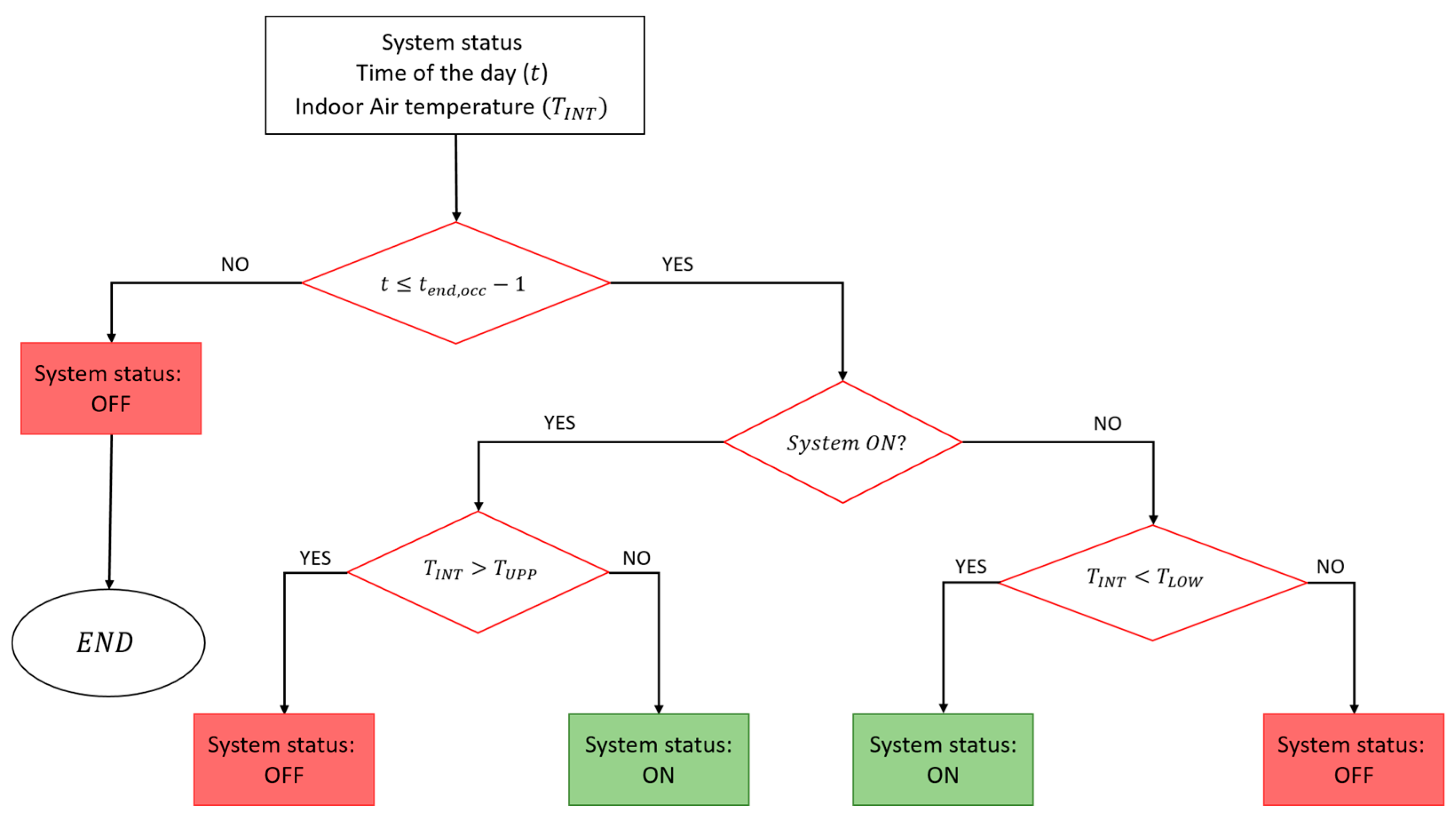
5.2. Rule-Based Baseline Control Logic
The performance of the DRL controller was evaluated against a baseline controller consisting of a combination of rule-based and climatic-based logics for the control of the supply water temperature of the considered heating system. The supply water temperature varies linearly from 40 °C to 70 °C when outdoor temperature ranges between 12 °C and 5 °C. These values were selected according to those implemented in the real Building Energy Management System (BEMS). This control strategy is in operation for up to one hour before the occupants leave the building (indicated as ). The RBC controller manages the boiler switch-ON according to the difference between the lower bound of the temperature comfort range and the actual indoor temperature, and the time before the arrival of occupants. Specifically, the boiler is switched-ON:
between four and three hours before the arrival of the occupants if the temperature difference is greater than 3 °C;
between three and two hours before the arrival of the occupants if the temperature difference is greater than 2 °C;
two hours before the arrival of the occupants if the temperature difference is greater than 0.
After the switch-ON of the heating system, the control logic follows the sequence illustrated in
Figure 4. The boiler is turned-OFF at any time when the indoor thermal zone temperature
is higher than the upper bound of the temperature comfort range
, equal to 22 °C.
In addition, if the zone is occupied and the temperature drops below the lower threshold limit temperature , equal to 20 °C, the system is turned-ON.
The boiler is set in the OFF condition on Sundays due to the office being closed.
5.3. Design of the DRL-SAC Control Logic
This section is focused on the design of DRL control algorithm, in order to define the action-space, the state-space and the reward function.
5.3.1. Design of the Action-Space
The action supplied by the controller is the supply water temperature value to the radiators. The action-space includes values between 20 °C and 70 °C and was expressed as a continuous space, since SAC was selected as the control algorithm. Hence, the action chosen is:
Moreover, the circulation pump is shut down if the chosen action is equal to or lower than 25 °C.
5.3.2. Design of the State-Space
The state-space is composed of a series of observations provided as inputs to the agent. The values assumed by the space-state variables influence the control action. The state-space was made of 52 features, reported in
Table 2, together with their lower and upper bounds. The variables chosen are feasible to be collected in a real-world implementation and provide to the agent the information necessary to predict the immediate future rewards. The
Indoor Air Temperature information during each control step was described as difference between the indoor temperature setpoint SPINT and the actual indoor air temperature TINT as directly linked to the reward formulation, as shown in
Section 5.3.3. This quantity is memorised in the state-space at the current control time step ∆
tcontrol and for three previous control steps, ∆
tcontrol,−1 (30 min before), ∆
tcontrol,−2 (1h before) and ∆
tcontrol,−4 (2h before).
Outdoor Air Temperature was included because it is the exogenous factor with the most significant influence on the heating energy consumption.
Occupants’ Presence status indicates if, in a certain control time step, the zone is occupied or not (based on the occupancy schedules) through a (0,1) binary variable. The two last features are saved in the state-space at the current control time step ∆
tcontrol and for all control time steps within the following 12 h. Observations were scaled within a range of (0, 1) in order to feed the neural network with min-max normalisation.
5.3.3. Design of the Reward Function
The reward function was formulated as a linear combination of two different parts, an energy-related term and the temperature-related term. They were combined employing two weights (δ and β, respectively) that were made to vary in order to change their importance.
Equation (6) describes the reward function r implemented in this work that the SAC algorithm exploits to learn the optimal control policy as introduced in equations form (1) to (4).
The energy term (
rE) refers to the heating energy consumption, calculated in kWh. The temperature term (
rT) was evaluated as the temperature difference between the upper/lower threshold temperature and the indoor air temperature evaluated in °C. The general expression of the reward is as follows:
The objective of the agent is to maximise the reward, with a maximum (ideal) value of zero. On Sunday, due to the absence of occupants, the reward value was set to zero.
The energy term of the reward is expressed in the following way:
where
EHEAT is the energy heating consumption for the current control time step.
The temperature term, on the other hand, has different expressions depending on the presence of occupants.
If no occupants are present, the temperature term is:
If occupants are present, the temperature term could have three different expressions:
This formulation of the temperature term was chosen to try to speed up the learning process and to avoid the exploration of unacceptable states from the beginning of the process.
5.4. Online Training Setup
The use of a DRL algorithm implies the selection of several hyperparameters that influence the behaviour and performance of the agent. To assess their influence, a sensitivity analysis was performed.
The hyperparameters involved in sensitivity analysis were:
temperature—term weight reward factor β;
energy—term weight reward factor δ;
learning rate μ;
gradient steps, which indicate the number of gradient updates after each step.
The weight factors help to define the relative importance of the two reward terms and therefore to determine the agent choices in investing greater attention to comfort instead of energy consumption.
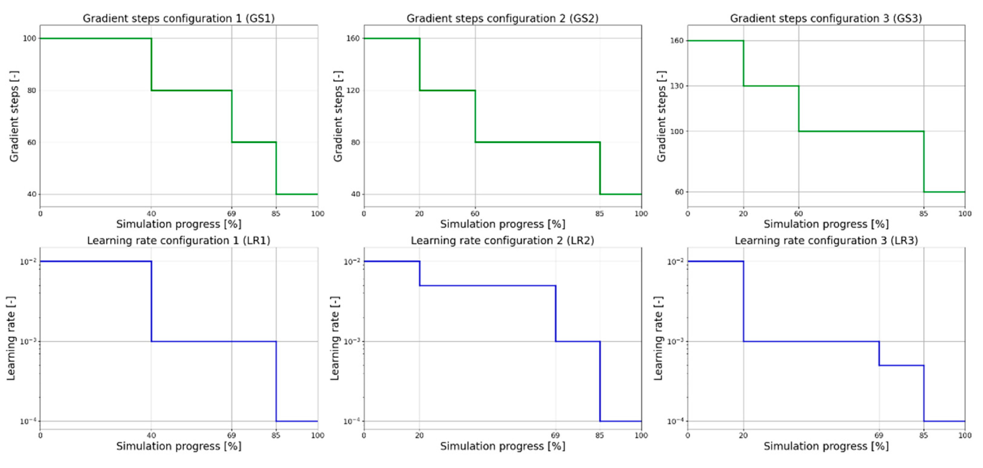
Three piecewise functions were defined for both gradient steps (GS1, GS2, GS3) and learning rate (LR1, LR2, LR3), as detailed in
Figure 5. The value of these two features decreased according to the percentage progress (between 0% and 100%) of the simulation. The choice of designing these two parameters as time-varying functions allows the optimisation of the online training.
At the beginning of the simulation, the DRL controller has no adequate background concerning the action to be chosen. For this reason, gradient steps and learning rate values were set higher, in order to facilitate the exploration process. As the simulation proceeded, both terms were decreased in order to allow the control agent to learn from the environment, but at the same time to not over-explore the space of the actions, as excessive exploration could cause a deviation from the optimal control policy that the agent might be able to learn at the beginning of the online training phase.
Within the set of hyperparameters, it was decided to keep those indicated in
Table 3 fixed. A four-layer feed-forward neural network was used, with 64 neurons per hidden layer. The deployment episode, repeated only once, as required when performing an online training, had a duration of three months, from 1 December to 28 February, for a total of 4320 control steps (90 days) and 25,920 simulation steps (every 5 min). On average, the episode took 60 minutes to be simulated on a machine with an 8th Generation Intel@ CoreTMi7-8550U @ 4.0 GHz processor and 16.0 GB RAM. The weather file used in this phase refers to the heating season 2018/2019.
The different configurations of hyperparameters tested are shown in
Table 4.
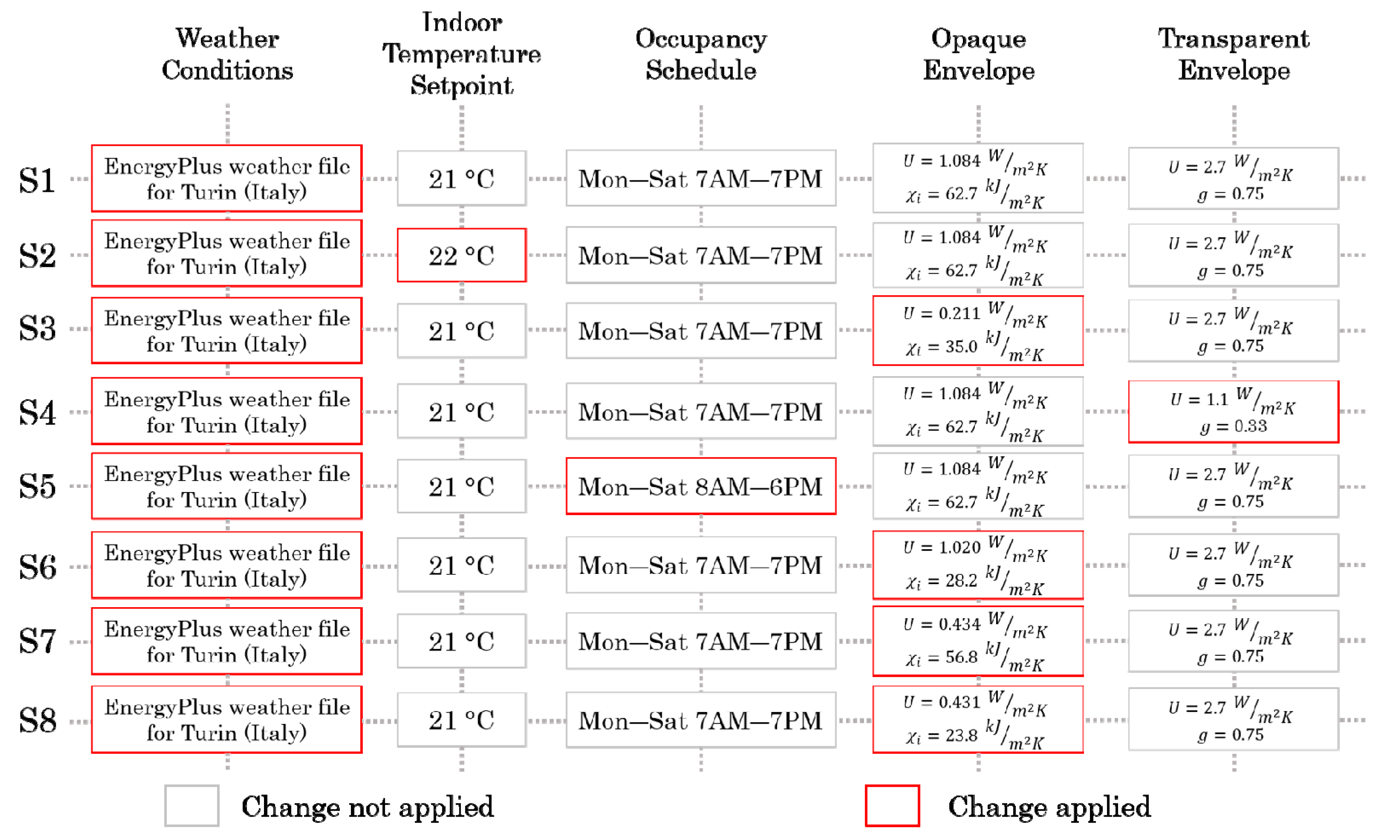
5.5. Scenario Analysis
The configuration considered to be the best among those explored during the online training phase was chosen for testing the adaptability of the agent in eight different scenarios, for the same simulation period as the online training phase but in a different climatic heating season. The scenarios considered include variation of outdoor conditions, building features (thermal transmittance, internal heat capacity, solar heat gain coefficient ), temperature setpoint and occupancy schedule. In detail, the weather file used in the online training phase was replaced with the reference weather file (ITA-TORINO-CASELLE-IGDG.epw) available in EnergyPlus for Turin (Italy) to test a different heating season.
The agent was deployed dynamically and statically:
in dynamic deployment, the RL agent is characterised by continuous learning as during the online training. For each control time step, the agent collects information about the state of the system, computes a control action, observes the reward value and the next state and then updates the control policy. In this case, the agent exhibits great flexibility to the continuous changing of system characteristics, indicating a good attitude in adjusting the control policy. On the other hand, this type of deployment requires higher computational cost, and the control policy may as a result be more unstable than the static case [
5];
in static deployment, the agent trained online was used as a static function. This process requires less computational time than the dynamic one, but the control agent needs to be re-trained when building features are changed in order to exhibit adaptive capabilities.
The DRL was deployed both statically and dynamically for each scenario and the performance achieved in these two cases was compared. The scenarios considered are summarised in
Figure 6.
6. Results
The results obtained by implementing the SAC control logic are presented in this section. Initially, the performance of the DRL agent in the online training phase was compared with the baseline. Afterwards, during the scenario analysis, the results obtained for the agents deployed statically and dynamically are highlighted.
6.1. Online Training
As reported in
Section 5.4, during the online training, a sensitivity analysis was preliminarily performed on some hyperparameters. Specifically, 16 configurations were evaluated, as shown in
Table 4. To assess the goodness of each configuration, suitable metrics were introduced and compared.
In detail, two metrics were selected during the period of operation:
the amount of energy needed for heating the supplied water to the terminals;
the cumulative sum of temperature violations during the occupancy hours, measured in °C.
A temperature violation occurred when, during the occupancy period, the temperature was not within the acceptability range (−1, 1) of the 21 °C setpoint. It was calculated as the absolute difference between the indoor temperature value and the lower or upper limit of the acceptability range, when the internal temperature was lower or higher than these limits.
The two metrics were evaluated for each simulation step and summed up at the end of the online training period. Moreover, the metrics were also calculated for the baseline to compare its performances with the DRL agent. The results obtained for the baseline and for the various configurations of hyperparameters are shown in
Table 5. The results indicate that some configurations (i.e., Run 12-13-14-16) accomplish the objective of reducing the heating energy demand and improving the control of indoor temperature during the occupancy period.
The most significant benefit was represented by the improvement of maintaining the indoor temperature within the predefined band. In that sense, the best result was provided by configuration 13, in which the cumulative temperature violations, for the entire deployment period, was equal to 121.9 °C. This value was reduced by more than 60% compared to the baseline case. At the same time, for configuration 13, a slight reduction in heating energy consumption was obtained in comparison to RBC baseline.
Therefore, the agent considered configuration 13 to be the best solution after the sensitivity analysis.
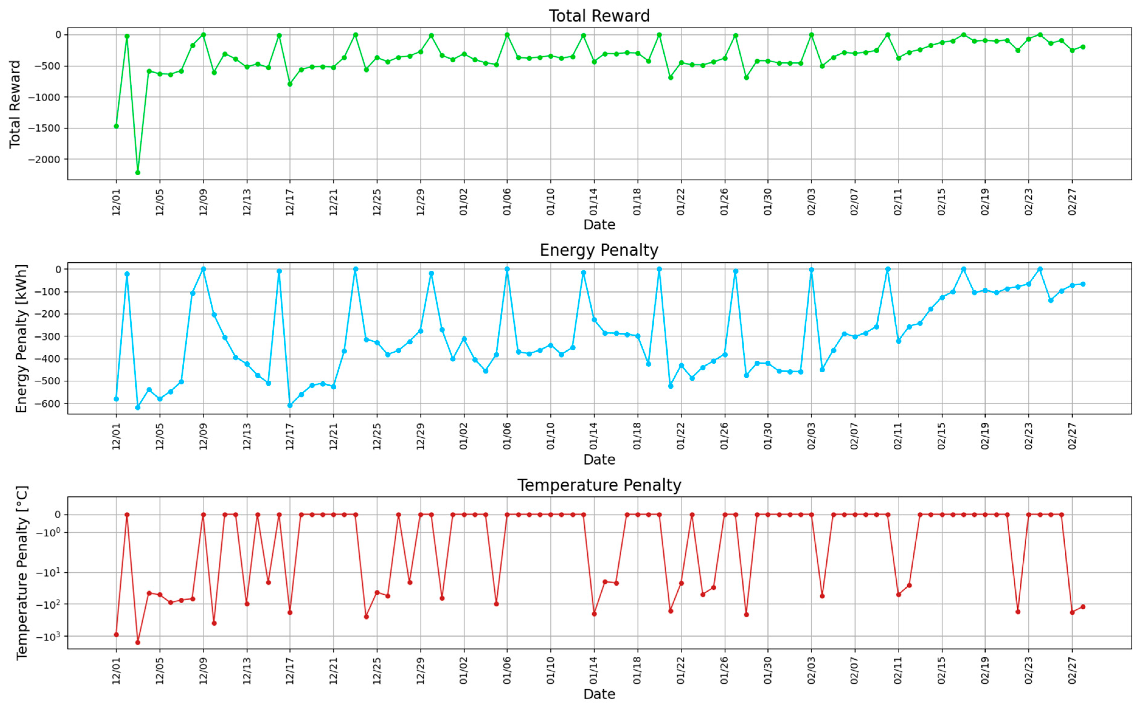
Figure 7 shows the cumulative reward evolution for this solution. The reward does not have a direct physical meaning, as it gives indications on the control policy convergence of the proposed agent. A non-convergent trend could cause instability of the optimal control policy.
Figure 7 is composed of three subplots. The top panel shows the cumulative total reward trend, while the two bottom panels report the evolution of the energy and temperature terms of the reward function. For the sake of clarity, the evolution of the temperature-term is reported in logarithmic scale.
The agent starts the exploration with relatively high values of the two terms of the reward. During the online training period, a recurring behaviour for both energy and temperature term can be observed. On Sunday, the reward was not computed, given the shut-down of the heating system due to the absence of occupancy; therefore, its value was set to zero, as highlighted in
Figure 7. On Monday, the two reward terms show a decrease due to the high amount of energy required to bring the environment to the desired temperature conditions and due to inability of the agent to guarantee these temperature conditions before the beginning of the occupancy period. During the last days of the heating season, the agent is able to better enhance the reward having gained experiences during the online training period.
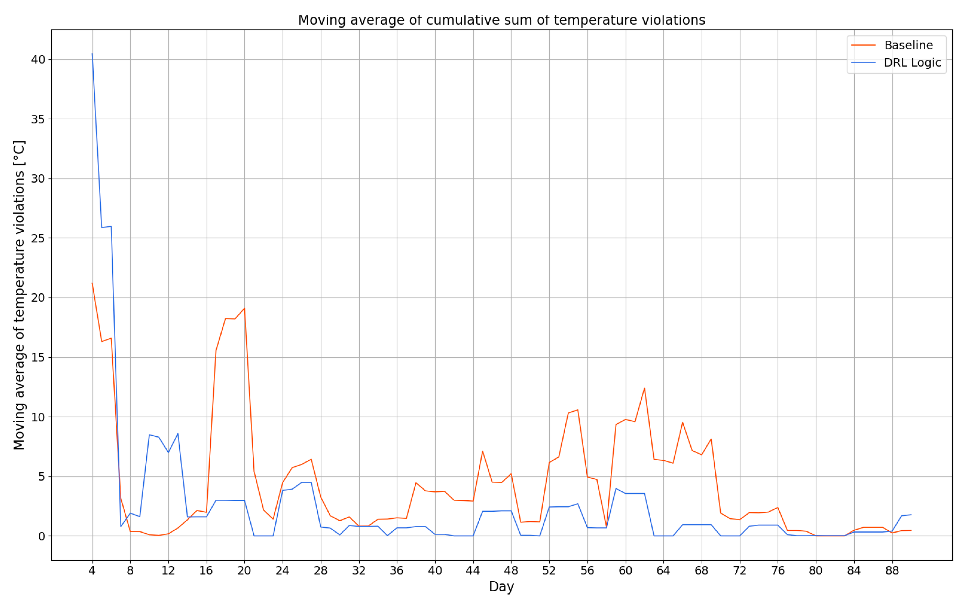
Training a DRL control agent online without any offline pretraining may require a large amount of time before the performance obtained can be considered acceptable. The moving average over a 4-day time window was calculated for the cumulative sum of temperature violations as shown in
Figure 8 to assess the time required for the best trained online DRL controller to perform similarly to the baseline. It was not necessary to calculate the moving average for energy consumption since it is similar as the baseline.
Figure 8 compares the moving average for the DRL agent and the baseline, starting from the first day of its availability, i.e., the fourth day of the training period. During the first stages of the training period, the baseline performs better than the model-free agent: for the latter, the moving average trend suggests that the learning of the optimal control policy starts from the second week of training. This choice implies that the action-selection during the first week is randomised; thus, it is useful for the preliminary exploration of the action space and not for the optimisation of the control strategy.
During the third week, the DRL agent outperforms the baseline in establishing the desired indoor temperature conditions. Hence, the timeframe required to achieve performance at least similar to the baseline resulted reasonable.
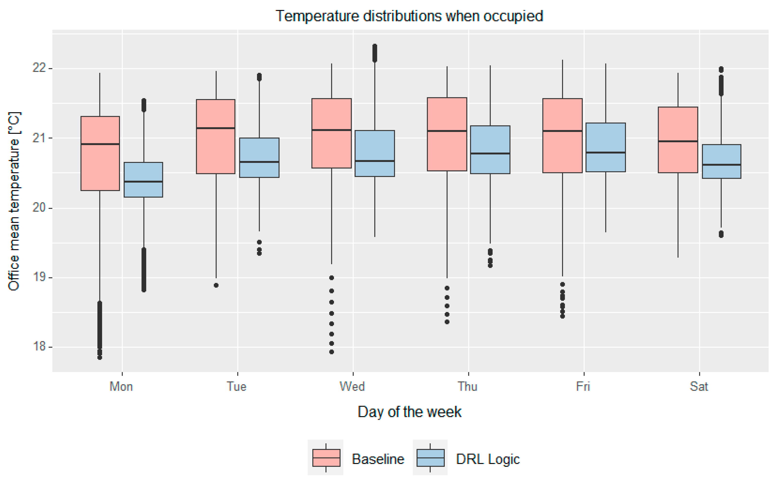
Figure 9 compares the indoor temperature distributions for the baseline and DRL control logic during the occupancy period for each day of the week. The baseline and the DRL control logic were compared considering as objective the same acceptability range for the indoor temperature.
The DRL controller is capable of better maintaining the indoor temperature within the acceptability range (with a lower value of temperature violations). In addition, the indoor temperature is mostly maintained with the DRL controller in the lowest part of the acceptability range.
The temperature distribution comparison for the two control logics shows that the indoor temperature has a smaller range around the setpoint in the case of the adaptive control strategy for every weekday.
6.2. Scenario Analysis
In this section, the results of the scenario analysis are reported, where the adaptability of the control agent selected in the online training phase was tested in the eight scenarios as proposed in
Figure 6. The deployment of the agent was simulated both dynamically and statically. As previously mentioned, a deployment episode runs for 90 days, including December, January and February. The meteorological file used is the reference one for Turin available in EnergyPlus, simulating the performance of the DRL control agent on a different heating season from the one considered in the online training phase.
Table 6 summarises the results obtained for baseline, static and dynamic deployment, for all scenarios with reference to energy consumption and cumulative sum of temperature violations during the whole heating season.
The SAC agent provided a great advantage in terms of control of indoor temperature especially in dynamic deployment. On the other hand, the results for energy consumption were opposite to the previous ones, as the dynamically deployed agent required more energy than the statically deployed agent and the baseline for all scenarios.
The dynamically deployed agent led to an increase of the heating energy need to reach the set point temperature conditions during occupancy that results in the reduction of temperature violations. Although the control strategy provided by the dynamically deployed agent led to an energy consumption over the entire period on average about 11% and 7% greater than the baseline and the statically deployed agent, respectively, it ensured an average reduction of 75% and 48% in terms of cumulative temperature violations. In particular, the temperature violations for the baseline controller refer indoor temperature values mostly below the lower bound of the acceptability range. This is the main reason for the lower energy consumption of the RBC controller.
In
Figure 10,
Figure 11 and
Figure 12, detailed results are reported for some scenarios, with the aim of highlighting the behaviour of the dynamically deployed agent and comparing it with the baseline or with the static counterpart.
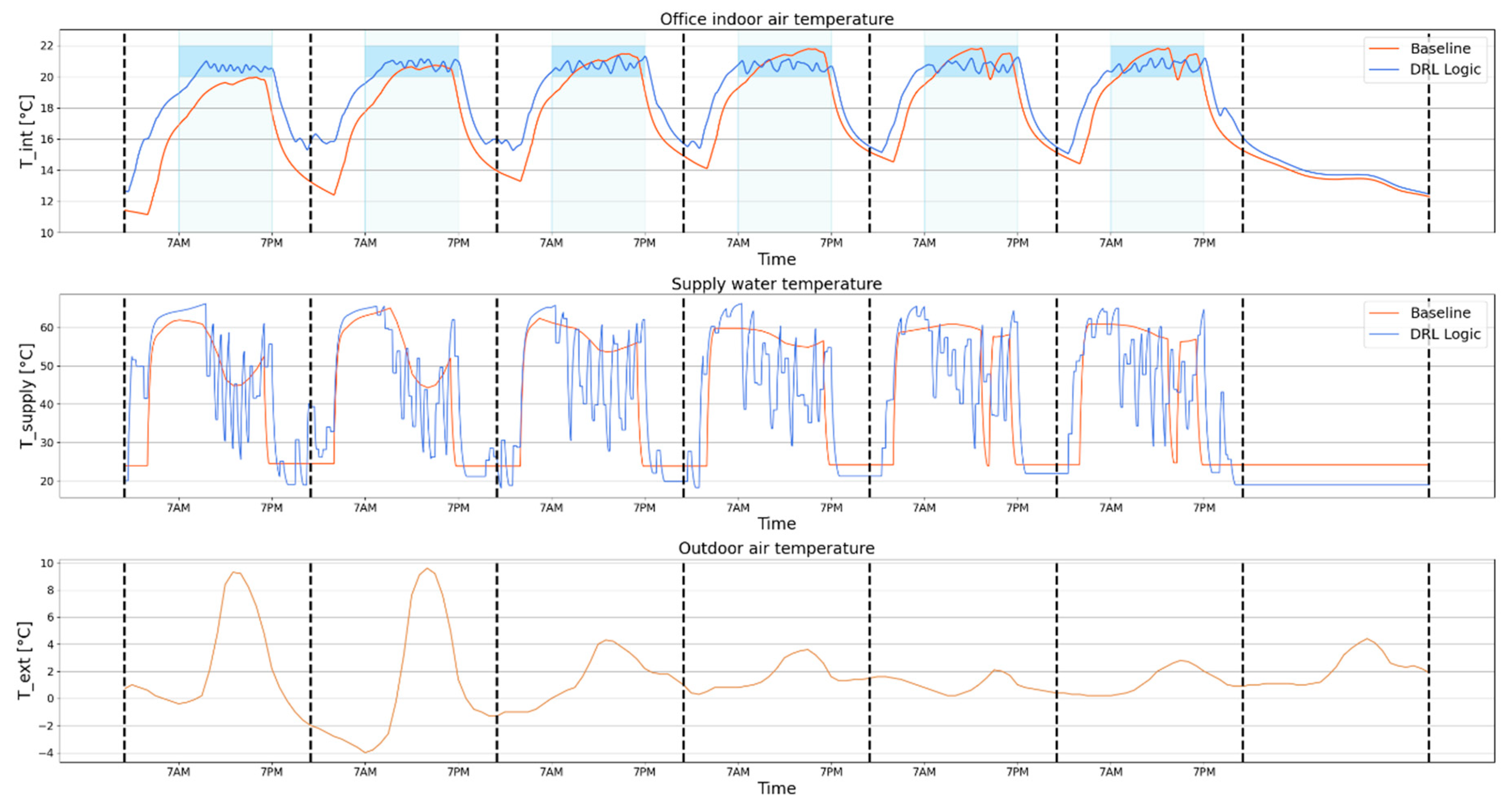
Figure 10 reports the comparison between the dynamically deployed and baseline control agent in scenario S1 during a typical week of the analysed period. The figure shows the indoor temperature patterns and the supply water temperature for these two controllers, along with the outdoor air temperature profile.
Monday is the most critical day, since during Sunday the heating system has been switched-OFF. Therefore, the indoor temperature during the first switch-ON phase on Monday is much lower than on the other days of the week: this requires careful management of the pre-heating phase to prevent the indoor temperature to fall outside the temperature range for comfort conditions on Monday, as occurred for the baseline controller highlighted in
Figure 10.
The adaptive control agent is able to reduce the temperature violations through an optimal management of the pre-heating phase maintaining the indoor temperature profile during the occupancy phase close to the lower part of the temperature band, to also limit the heating energy demand.
On other weekdays, the SAC agent succeeds in avoiding temperature violations respect to the baseline agent which, instead, reports violations during the first occupation phase. Above all, this phenomenon could be attributed to the flexibility of the agent concerning outdoor temperature conditions, since the agent receives information about the outdoor temperature pattern for the 12 h ahead the control time step considered. Therefore, the agent keeps the heating system ON until the end of the occupancy phase of the day, considering that the outdoor temperature was lower in the early morning, as can be observed from the supply water temperature values shown in
Figure 10. In this way, the dynamic deployment manages the switch-ON phase better than the baseline, avoiding temperature violations during the first hours of occupancy period.
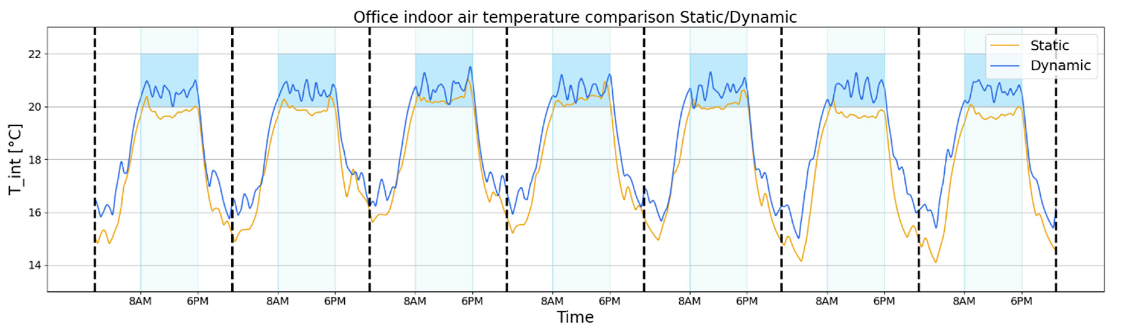
Figure 11 compares the indoor temperature patterns resulting from the statically and dynamically deployed agents during a week in the scenario S5. In this scenario, the building is also occupied on Sundays, and the occupancy period is restricted to between 8 AM and 6 PM for all weekdays. The static agent is not able to handle the change of occupancy schedules, and therefore to change the control policy learned during the online training phase. As reported in
Table 6, the cumulative sum of temperature violation is much higher than that of the agent deployed dynamically.
On the contrary, the dynamically deployed agent is able to learn the change of occupancy patterns and optimises the control policy. Then, the required indoor temperature conditions during the occupancy are satisfied and temperature violations on all weekdays are reduced.
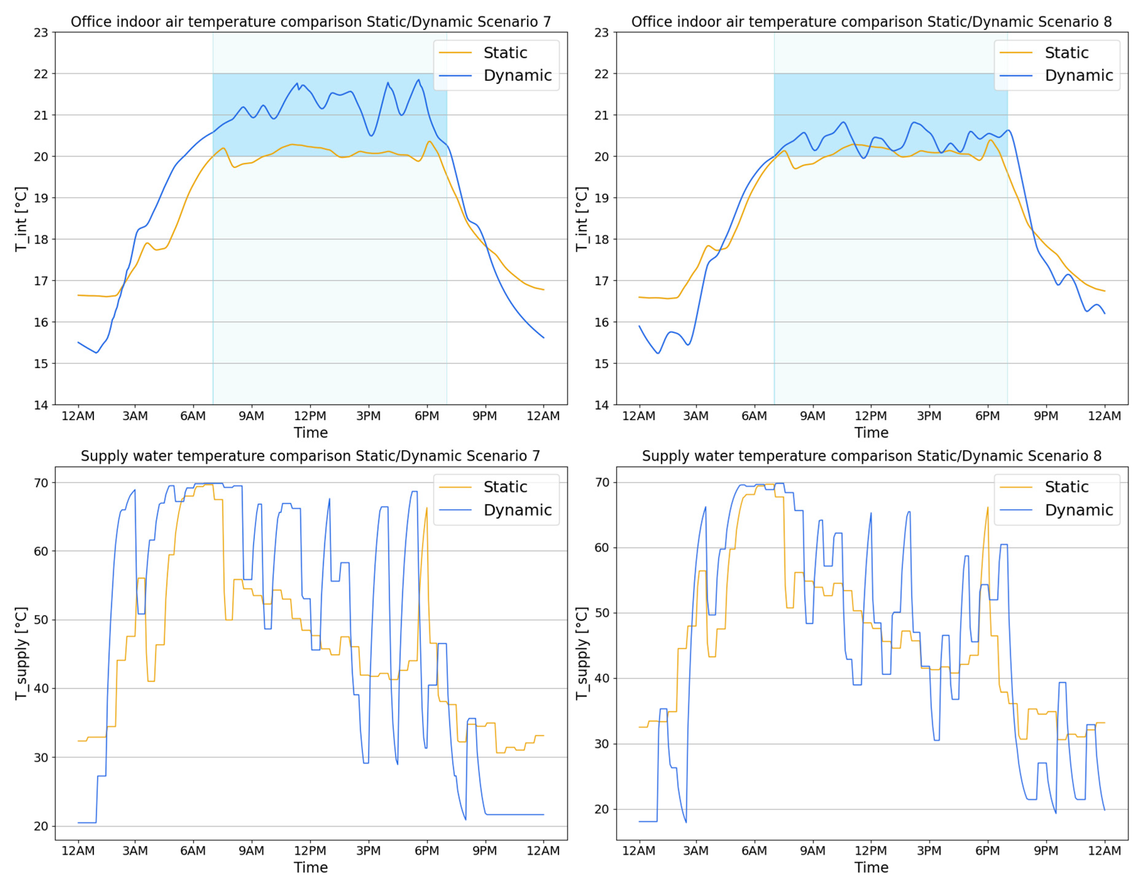
To conclude the scenario analysis, the indoor temperature profile and the supply water temperature in Scenario S7 and S8 are compared for the statically and dynamically deployed agents, as shown in
Figure 12, in order to demonstrate the flexibility of the agent when opaque envelope characteristics are modified.
In scenarios S7 and S8, the stratigraphy of the vertical walls was modified introducing respectively a massive and a light curtain wall. These changes aim to highlight the differences related to the internal heat capacity value considering that the thermal transmittance value were kept almost equal for the two cases. The adoption of a massive wall for vertical walls provides a significant internal thermal capacity than the light curtain wall, as can be seen in
Figure 6.
As stated previously, the static agent is not able to handle the change in boundary conditions, as demonstrated by the analysis of indoor temperature and supply water temperature profiles, which are identical in Scenario 7 and 8.
On the other hand, the dynamically deployed agent shows excellent flexibility with respect to changing the opaque envelope features. The agent was able to exploit the charging/discharging of thermal mass in both scenarios, anticipating the switch-ON time in the massive wall case. At the same time, the presence of a massive wall involves an advantage in terms of the heat accumulated. It makes it possible to avoid the system working until the end of the occupancy period, ensuring at the same time the required indoor temperature conditions.
The heating system is switched-ON about two hours in advance in the massive wall to allow an adequate charge of the mass and switched-OFF two hours in advance in order to better exploit the discharged heat. For both scenarios, the dynamically deployed agent allows the indoor temperature conditions required for the environment to be met, thus improving the performance compared to the static counterpart.
7. Discussion
This paper focused on the development of an adaptive model-free control strategy for a heating system that serves a real office building, whose current implemented control strategy consists in a climatic rule based one. This case study has particular importance, since the majority of non-residential buildings in Italy are equipped with this type of heating system.
The goal of this work was to train a DRL control agent online to maintain adequate temperature conditions during the occupied period and reduce the heating energy demand. For the developed controller, it was used a DRL algorithm based on a continuous action-space, named Soft Actor-Critic.
The DRL controller was deployed, for a calibrated energy model, in a simulation environment coupling EnergyPlus and Python.
It was chosen to perform an online training to emphasise the model-free nature of reinforcement learning. The online training of the DRL agent was able to guarantee performance improvements compared to the baseline, mainly in terms of indoor temperature control.
A sensitivity analysis was carried out during the online training phase, due to the strong dependence of the DRL controller performance on hyperparameters. The absence of guidelines providing support for the immediate choice of the hyperparameters of the algorithm implied the necessity of conducting this kind of analysis. As a consequence, despite the model-free nature of reinforcement learning, a modelling effort was required to analyse the impact of the hyperparameters in the performance of the controller.
The online training of the DRL controller may imply the occurrence of a discomfort period in the early learning stages, depending on the quickness at which the control agent learns an optimal control strategy. To obtain optimal performance faster, two hyperparameters of the algorithm, (i.e., gradient steps and learning rate) were assumed to be decreasing piecewise functions, in order to ensure higher values at the beginning of the simulation and guaranteeing the speeding up of the learning process. This strategy led to performances similar to those obtained with the RBC baseline after two weeks in the simulation period. As the simulation proceeded, these parameters were reduced in order to allow the agent to learn by interacting with the environment, avoiding over-exploration that could have caused deviation from the optimal control policy.
The best online training of DRL agent was then used for a subsequent scenario analysis, useful for testing the flexibility of the SAC control logic for the same period (including December, January and February), changing some boundary conditions, such as external weather conditions, occupancy schedules, structural conditions and indoor comfort conditions. These changes were grouped into eight different deployment scenarios.
During the scenario analysis, the higher heating energy demand associated with the dynamically deployed agent was justified by the significant improvement obtained in the indoor temperature conditions compared to the statically deployed agent and the baseline controller.
Compared to the static case, a dynamic deployment needs more computational time to complete the simulation due to the online update of the control strategy obtained from the training phase. The obtained results suggest that this kind of deployment is better able to handle changes in the controlled environment, highlighting its high potential for providing adaptive control policy. However, dynamic deployed DRL agents are more exposed to control instability issues that can compromise the identification of an optimal policy. For this reason, in this study, a proper analysis for the setting of agent hyperparameters was performed, thus also preventing the occurrence of significant deviations from the optimal control strategy during dynamic deployment.
8. Conclusions and Future Works
In this paper, the online implementation of an agent based on Soft Actor-Critic was evaluated for the control of a water-based heating system serving an office building. It was necessary to use a simulation environment to test its performance on a calibrated energy model.
After performing a sensitivity analysis on the hyperparameters of the SAC algorithm during the online training phase, the best agent was selected. In particular, it was able to reduce the cumulative sum of temperature violations by more than 60% with respect to the baseline controller.
A scenario analysis was then performed to test the flexibility and adaptability of the controller to the variation of different boundary conditions grouped within eight deployment scenarios. For this purpose, the agent was tested both statically and dynamically.
The best DRL agent was more effective when deployed dynamically in terms of indoor temperature control, with a reduction of the cumulative sum of temperature violations of about 50% and 75% in comparison to static deployment and rule-based control respectively. However, the dynamically deployed agent led to a heating energy consumption about 7% and 11% higher than the statically deployed agent and the baseline respectively. This trade-off is still reasonable, considering that the building’s indoor temperature conditions were remarkably improved when considering a dynamic deployment of the agent.
Future works will be focused on the following aspects:
The developed controller will be implemented in the real world, although switching from simulations to implementation is very complicated and still represents one of the main challenges, especially concerning infrastructure to make the controller available. The building’s heating energy requirements were evaluated using building energy simulation software (Energy Plus), assuming that the air was in ‘perfect mixing’ conditions. However, during the real implementation, the location of the indoor temperature sensors should be carefully defined, considering that the perfect mixing hypothesis could be not verified.
The SAC control logic will be tested with more modern HVAC systems, including renewable energy sources and energy storage.
The indoor thermal comfort will be evaluated by means of Predicted Mean Vote (PMV) and Predicted Percentage of Dissatisfied (PPD), including them in the objective function [
40,
41].
The aspects of reproducibility and standardisation will be further analysed, as the control agent implemented in this case study could perform differently for different HVAC systems or for buildings located in other climatic zones.


