Experimental Study of a Coil Type Steam Boiler Operated on an Oil Field in the Subarctic Continental Climate

Abstract

Transportable boiler plants are widespread in the northern regions of the Russian Federation and have a large and stable demand in various spheres of life. The equipment used and the schemes of existing boiler plants are outdated—they require replacement and modernization. Our proposed new installation includes a coil type steam boiler and ancillary equipment designed with the identified deficiencies in mind. The steam boiler coils are coaxial cylinders. The scope of the modernized transportable boiler plant is an oil field in the subarctic continental climate. The work is aimed at completing an experimental and theoretical study of the operation of a coil type steam boilers under real operating conditions. Experimental data on the operation of boiler plants are presented. The dependences of the fuel consumption of boiler plants on the temperature and pressure of the coolant are obtained. Statistical analysis is applied to the collected data. Conclusions are formulated and a promising direction is laid out for further research and improvement of coil type steam boilers. Equations are proposed for calculating the convective component of radiant-convective heat transfer in gas ducts, taking into account the design features of boiler units by introducing new correction factors. Comparison of the calculated and experimental data showed their satisfactory agreement.

1. Introduction

1.1. Operating Conditions of the Installation

Transportable boiler plants (hereinafter referred to as TPBs) are widespread in the subarctic continental climate of the Russian Federation and are in demand in various spheres of life: servicing private houses in cities and small remote settlements, in industry, and in oil production.

Relative to the subarctic continental climate conditions on the Köppen world map [1], TPB can be used in the D_fc zone. According to the climate classifier for specific conditions defined by Köppen [2] and the feasibility study for the use of renewable sources according to the climate classification by the same author [3], it follows that in addition to organic fuel, stationary or mobile wind turbines can be used in such conditions.

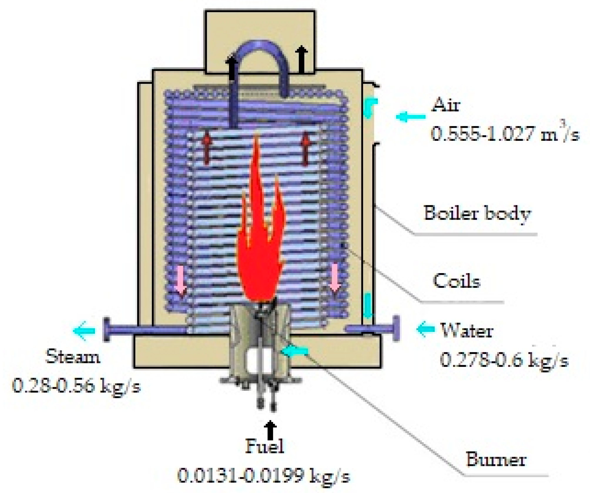
At drilling sites that specialize in oil production, steam and hot water are required for the technological and individual needs of the maintenance personnel. Oil fields in Russia are often equipped with block-modular boiler houses (hereinafter referred to as BMB) installations based on E-1.0-0.9 M(Z) boilers, which run on liquid fuel. Fuel consumption at nominal mode is 0.28 kg/s. The working pressure of the coolant on the manifold averages 0.4–0.45 MPa at a temperature of 143 °C (416 K). On the drilling rig, saturated steam is used to heat the equipment and technological processes. The boiler room provides the necessary steam parameters. There is no degasser in the usual form as for conventional boilers, but a separator is installed after the boiler and is a vertical pipe with a diameter of 250 mm, which includes steam-draining pipes from the boiler and pipes exit to the consumer. The separator also acts as a steam collector. Steam enters the separator from the boiler at high speed. Under the action of centrifugal forces, water droplets and sludge are separated and move down, and steam enters the steam lines to the consumer. Condensate accumulates in the lower part of the separator, which is returned to the feed tank via a separate pipeline. It is possible to clean the separator from the sludge by removing the bottom cover. Condensate that enters the feed water tank with a temperature of no more than 100 °C, which has a positive effect on heating the feed water and on the cost of their own needs in the harsh conditions of the north. The condensate in the tank is mixed with water coming from the water treatment plant. In the tank, water is stored at a temperature of no more than 50 °C, since feed pumps have a limit on the characteristics of the working medium.

In such boiler plants, there is a certain amount of necessary auxiliary equipment (chemical water treatment system, feed pumps, fans), which requires repair, replacement, and modification. The chemical water treatment system of such plants (hereinafter referred to as the CWT) does not cope with hard polluted water, putting it at risk and increasing the likelihood of boiler failure due to pipe fouling and burnout. Our experimental and theoretical work involves the modernization of TPB (hereinafter referred to as MTPB), and in particular the complete replacement of boilers, what is mentioned in the work Bennett [4].

1.2. Review of Works on the Research Topic

Companies offer compact steel units with fully automatic control, making it possible to operate units on different combined types of fuel thanks to the use of modern burners. For example, Bennett in the work [5] indicates the possibility of increasing the efficiency of boiler units through the use of upgraded burner devices. Sweetnam in the study [6] indicated that it is quite possible to increase the efficiency of home boiler units by burning various fuels, including natural gas and pellets. Both researchers, Bennett in [5] and Sweetnam in [6], noted the importance of the design of burner devices, as well as the combination of heat generation by the boiler unit and renewable energy sources to reduce the harmful impact on the environment. The boilers are designed for domestic and industrial use and meet emissions standards.

Modern boilers are competitive with their counterparts from manufacturers all around the world. For example, Hernández Corona et al. touched upon the main points of the boiler unit operation regarding its efficiency [7]. In [8], Guidez and Prele described steam generator designs similar to those considered in this article. Sharma et al. considered modified heat exchangers based on standard boilers [9]. Astorga-Zaragoza et al. [10], they drew attention to interesting facts about the use of steam generators in thermal power plants. Silva et al. in [11] conducted computer simulations similar to those considered by the Cheridi et al. [12]. The authors would also like to mention some works on topics similar to the one under consideration. For example, Moghari et al. [13] considered modeling of hydrodynamics in a boiler, while Sunil et al. [14] considered modeling, new techniques and their validation for the movement of water and steam in the boiler drum. Hag’s research [15] focuses on the evaporation processes for a steam generator, and Backi’s paper [16] uses a similar model. Despite the significant competition, domestic boilers are in great demand, both among large enterprises and among small consumers for a number of reasons.

Firstly, imported devices, distinguished by their ergonomic design, are more expensive to obtain and install, since all components of such boilers must be produced by the same manufacturer. Lower-priced analogs are not always suitable for their technical characteristics.

Bruce-Konuah et al. [17] considered the issues of energy saving in boiler installations and heat supply systems at residential facilities, and also pointed out the shortcomings of hot water boiler units. Dixon and Nguyen [18] studied forecasting algorithms, models of hot water and steam production systems, and came to the conclusion that there are opportunities to optimize the design of boilers and heat supply systems. Kusumastuti et al. [19] considered the processes of vaporization and injection of condensate into steam to change its parameters and came to the conclusion that the systems of vaporization and steam supply require improvement.

Secondly, imported boilers cannot operate efficiently with unstable fuel supplies and require very high quality feed water, and, as a result, the cost of installation increases.

Russian boilers have a number of other advantages that make them competitive in the domestic market: low cost compared to foreign analogues; simplicity and ease of use; their design and installation take into account the peculiarities of operating conditions, including the climatic conditions of Russia; compliance with Russian regulations and standards; high maintainability; reliability and ability to operate boilers longer than planned; possibility of custom ordering and installation for special projects; possibility of troubleshooting issues identified during operation with the manufacturer. Badur and Bryk [20] considered the use of low-pressure steam obtained from the boiler unit in a low-power turbine. At the same time, Duarte et al. [21] showed the possibility of applying reliability criteria to power equipment that contribute to trouble-free operation, including boiler units that produce low-pressure steam.

Russian manufacturers design and manufacture equipment that meets modern standards and consumer requirements, which increases demand. There is a trend to improve the automation and materials used in the main components of boilers. Manufacturers are paying more attention to the fuel used, the combustion process, and environmental aspects. The use of domestic components in boilers facilitates the replacement and repair of failed parts, which has a positive effect on the production of Russian steam generators, since the foreign analogues of components cost several times more and delivery times for such parts are much longer.

In connection with the listed advantages and further development prospects of the domestic market for the production of water-tube coil and fire-tube boilers, we chose a coil-type steam boiler produced in the Urals. The characteristics of the boilers developed by the authors were compared with the analogues presented by Chauhan and Khanam [22], dedicated to mini thermal power plants with low-pressure steam generators or Shi and Wang [23], in which a boiler of a similar type operating on solid fuel is considered.

1.3. The Design of the Steam Generator under Consideration

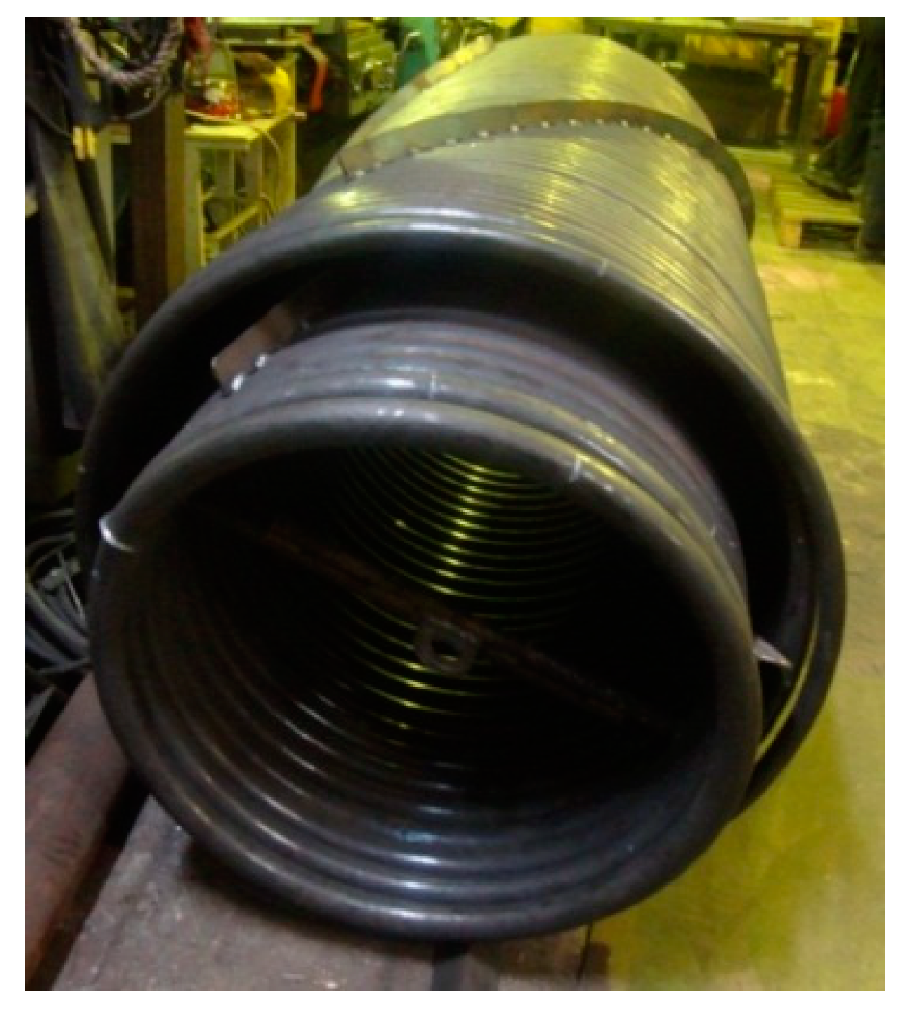
An upgraded transportable boiler plant was designed for the experiment. The main equipment is coil-type steam boilers (Figure 1). The installation consists of all the necessary main and auxiliary heating and electrical equipment. The MTPB is housed in a modular marine type container and is designed to operate in cold climatic conditions. Our experiment involves the collection and analysis of the performance parameters of a coil-type steam boiler in the real operating conditions of the Far North. The installation to be studied is located at the cluster site of the Var-Yogan field in the winter heating season. We set a number of tasks to achieve our research goals: supply steam to the drilling rig and auxiliary units for heating equipment and the technological process of collecting basic data on the operation of a steam boiler; construction and analysis of dependences of temperature and steam pressure on fuel consumption, on qualitative and quantitative parameters of feed water to justify economic and technical costs, advantages, and further prospects in the research and design of boiler houses, what is noted in the work of Kuznetsov et al. [24].

2. Materials and Methods

The temperature, pressure and velocity measurements in the diagram in Figure 2 were carried out according to the methods approved in the Eurasian Economic Union. However, the authors were also guided by the recommendations of the European Union in the field of measurement uncertainty and the methodology used. Measuring devices that were installed in the experimental boiler room according to Figure 2: pressure gauges showing in place and electric contact, Karat-520 water flow meter (produced by the limited liability company “Uraltechnologiya”, a member of the NPO KARAT group of companies, Yekaterinburg City, Russia), Petroll fuel meter (“Petroll” company, Moscow, Russia), thermocouples for measuring the temperature of steam and gases in different parts of the coils, testo-320 gas analyzer (German Corporation Testo SE & Co. KGaA, Lenzkirch, Germany) for analyzing the composition of flue gases. With the help of the above devices, the main parameters were measured for steam (pressure and temperature), water and fuel consumption, as well as the main indicators for flue gases (temperature, O₂).

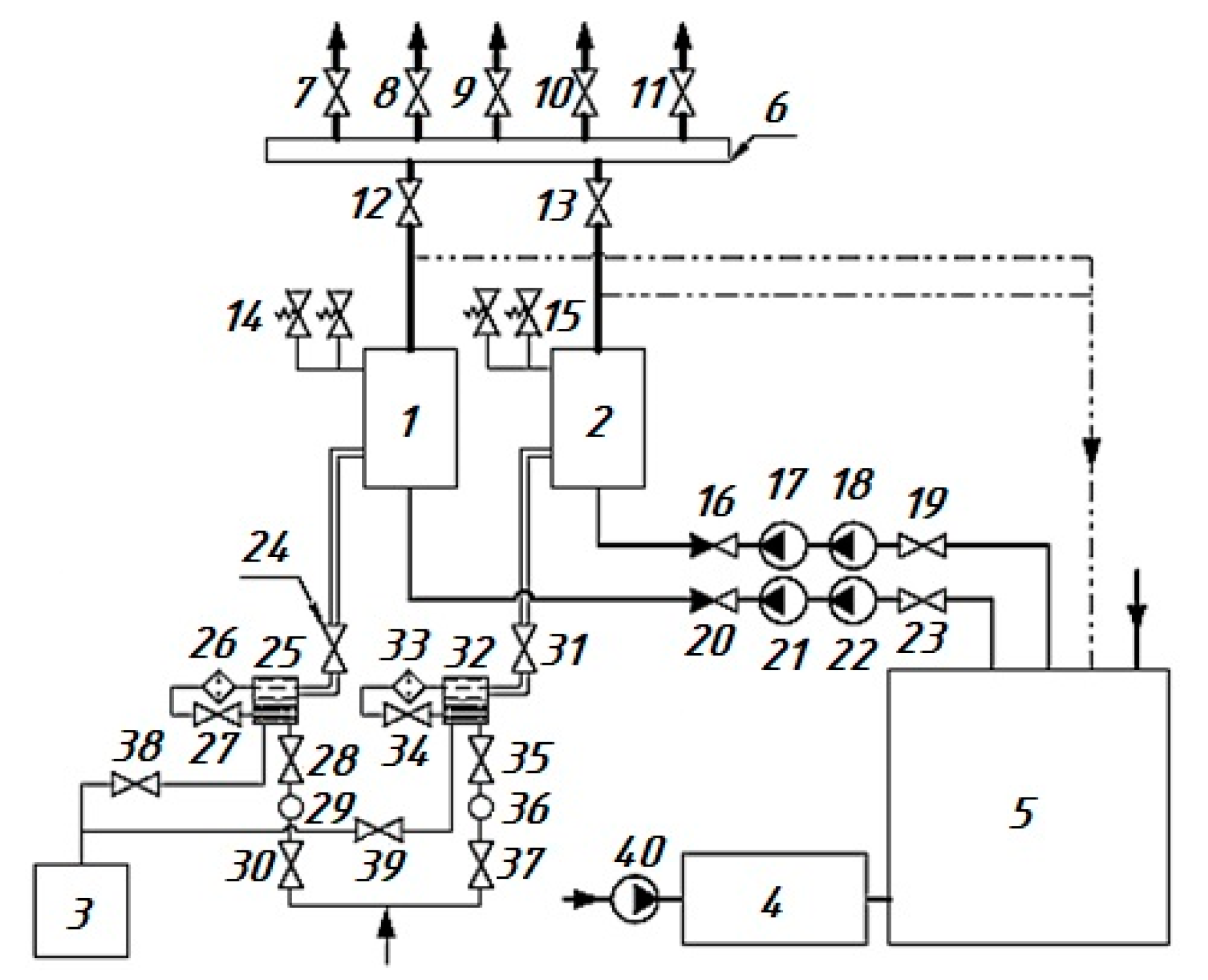
During operational testing, the MTPB was operated in two modes to compare the results. A schematic diagram of the MTPB is shown in Figure 2. The first mode represents the operation of one boiler (in Figure 2, Symbols 1 and 2) and feed pumps (in Figure 2, 21, 22 and 17, 18) in turn.

The development of the experimental research methodology is based on the estimation of the uncertainty arising from each of its sources. For example, the diagram in Figure 2 shows devices for measuring flow, temperature, and pressure. To determine the total uncertainty, you need to define each one separately, and then use the formulas for the constructed model.

In the case of the authors’ research, the method itself contributes to the uncertainty, so this contribution can be expressed as a value that affects the final result. In this case, the uncertainty of the parameter is expressed directly in units of y, and the sensitivity coefficient ∂y/∂x = 1.

The result of the steam velocity measurements—the arithmetic mean of 4.147 m/s is characterized by a standard deviation of 0.04 m/s. The standard uncertainty u(y) associated with precision under these conditions is 0.04 m/s. The model of this measurement in this case can be expressed by the formula y = (calculated result) + ε, where ε reflects all random effects under the given measurement conditions, with the sensitivity coefficient ∂y/∂x = 1.

Calculate the arithmetic mean of the steam velocity from all measurements at a given point:

$$\mathrm{w}=\frac{1}{\mathrm{n}}{\displaystyle \sum }_{\mathrm{i}=1}^{\mathrm{n}}{\mathrm{w}}_{\mathrm{i}}$$

(1)

After calculations using Equation (1), we get the value w = 4.147 m/s.

For sources of random uncertainty, we calculate the uncertainty by type A:

$${\mathrm{u}}_{\mathrm{A}}\left(\mathrm{w}\right)=\sqrt{\frac{{\sum }_{\mathrm{i}=1}^{\mathrm{n}}({\mathrm{w}}_{\mathrm{i}}-\mathrm{w})}{\mathrm{n}\left(\mathrm{n}-1\right)}}$$

(2)

Calculations using Equation (2) gave the result ${\mathrm{u}}_{\mathrm{A}}\left(\mathrm{w}\right)=0.8\%$.

For sources of systematic uncertainty (instrument error) calculating the uncertainty by type B:

$${\mathrm{u}}_{\mathrm{B}}\left(\mathrm{w}\right)=\frac{∆\mathrm{w}}{\sqrt{3}}$$

(3)

Calculations using Equation (3) gave the value of ${\mathrm{u}}_{\mathrm{B}}\left(\mathrm{w}\right)=1.58\%.$

Calculate the total standard uncertainty:

$${\mathrm{u}}_{\mathrm{C}}\left(\mathrm{w}\right)=\sqrt{{\mathrm{u}}_{\mathrm{A}}{\left(\mathrm{w}\right)}^2+{\mathrm{u}}_{\mathrm{B}}{\left(\mathrm{w}\right)}^2}$$

(4)

Using Equation (5), we get the value ${\mathrm{u}}_{\mathrm{C}}\left(\mathrm{w}\right)=\sqrt{0.64 + 2.4964}=1.771\%.$

For the confidence probability (coverage probability) P = 0.95 (it is recommended in the Manual calculation of uncertainty) setting the coverage factor k = 2 and calculate the extended measurement uncertainty:

$$\mathrm{u}={\mathrm{ku}}_{\mathrm{C}}\left(\mathrm{w}\right)$$

(5)

Finally, the total value of the extended uncertainty is$\mathrm{u}=2·1.771=3.542\%$. The total value of the extended uncertainty is$\mathrm{u}=2·0.01=0.02 \mathrm{MPa}$ in case of k = 2. The purpose of using u is to show the confidence interval of the uncertainty band near the pressure measurement result, within which one can expect to find most of the distribution of pressure values that could reasonably be attributed to the measured value.

According to the Guidelines for measurements and their uncertainties in the countries of the Eurasian Economic Union, a maximum value of 5% is accepted for experimental data, so the results obtained fall into the confidence interval.

The found uncertainty value is subject to revision only in the process of revalidation of the analysis methodology. Validation of the measurement method was carried out during repeated tests of the boiler unit in the conditions of operation at the oil and gas field in the far north. To ensure that the performance indicators obtained during the development of the methodology are achieved with its specific application, the methodology is validated. In the case of the author’s research, the technique was conducted in an interlaboratory study, which resulted in additional data on the effectiveness.

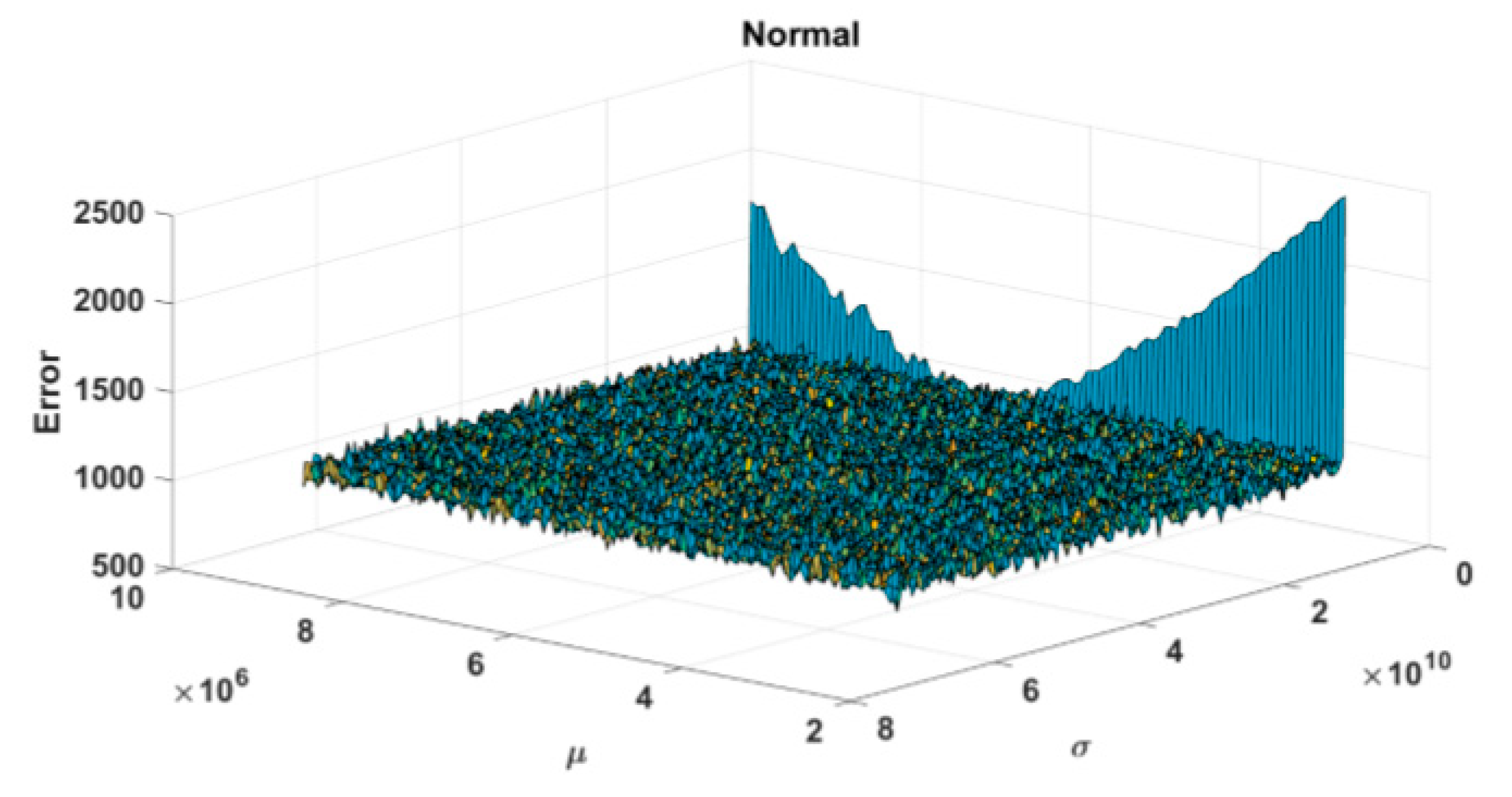
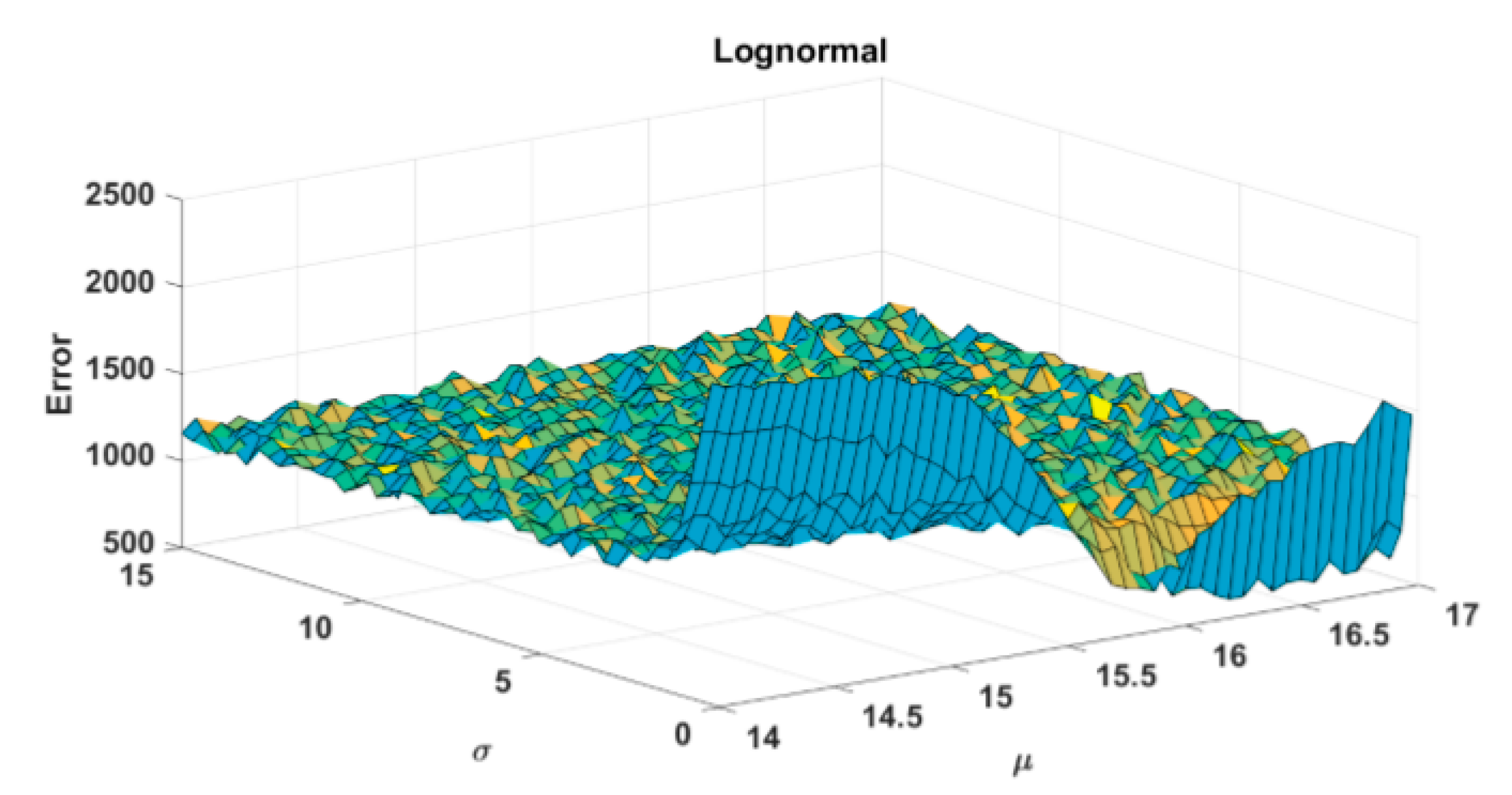
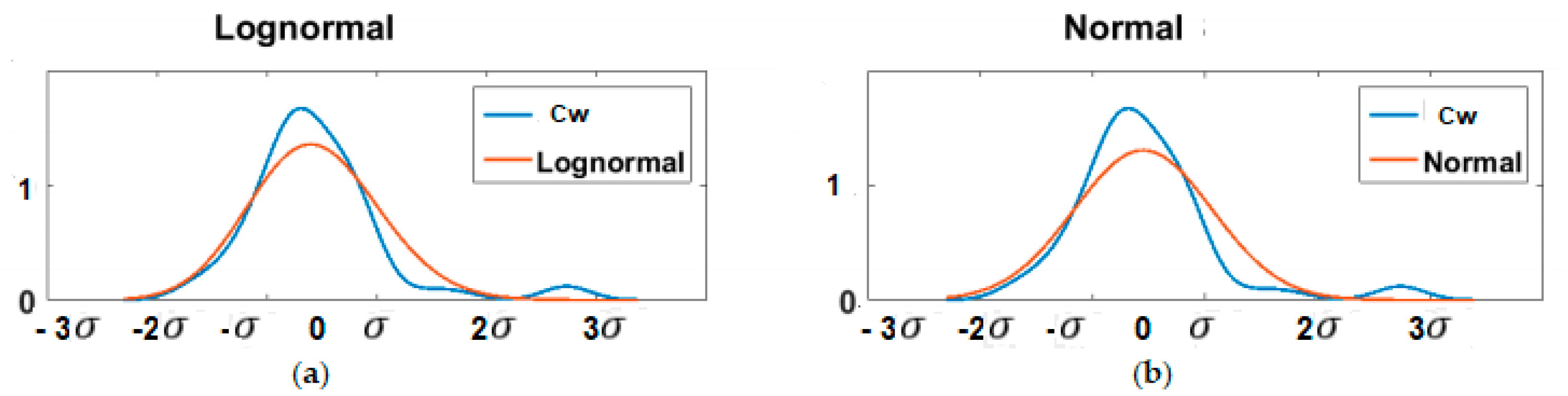
At this stage, we know the distribution functions of all the parameters of the model, so, assuming that the parameters correspond to the distribution functions, we calculated the validation error shown in Figure 3 and Figure 4, and Error = 895.5186 (Normal), Error = 177.7951 (Lognormal). Charts are made using MatLab (MathWorks developer, Natick, MA, USA).

Similarly, the uncertainty of other variables, such as temperature and pressure, was evaluated. The calculated value of the correction introduced in the measurement result, necessary to take into account the influence of the heat sink on the thermometer body and the thermal resistance between the sensor element of the thermometer and the channel wall, is 0.025 °C. The uncertainty of the correction value using thermal modeling lies in the range from 0.005 to minus 0.005 °C. There are reasons to assume that the probability density of uncertainty has a uniform distribution. The certificate of verification of the used measuring device indicates its confidence error is equal to 0.01 °C with probability 0.95 (2σ).

Thus, we consider the case of direct measurements, which does not require the representation of the measured value in the form of a functional dependence. In this case, the uncertainty of the measurement result can be represented as the sum of the uncertainties caused by the influence of various factors, which can be determined on the basis of all available information. At the same time, it can be assumed that all the components of uncertainty are not correlated. The following sources of uncertainty of the measurement result can be determined from the experimental condition:

(1)

Random component of the thermometer reading T_i, caused by a random change in all possible effects affecting the measurement result.

(2)

Inaccuracy of the method for estimating the correction introduced to account for the effect of the heat sink effect on the thermometer body.

(3)

The probabilistic nature of the estimation of the error of the thermometer. Total standard uncertainty ${\mathrm{u}}_{\mathrm{C}}\left(\mathrm{T}\right)$ of temperature measurement can be described by the following relation:

$${\mathrm{u}}_{\mathrm{C}}\left(\mathrm{T}\right)=\sqrt{{\mathrm{u}}_{\mathrm{A}}{\left(\mathrm{T}\right)}^2+{\mathrm{u}}_{\mathrm{B}1}{\left(\mathrm{T}\right)}^2+{\mathrm{u}}_{\mathrm{B}2}{\left(\mathrm{T}\right)}^2}$$

(6)

where ${\mathrm{u}}_{\mathrm{A}}$—estimation of the random component of the total uncertainty of the temperature measurement result, estimated by type A; ${\mathrm{u}}_{\mathrm{B}1}$—estimation of the uncertainty component of the temperature measurement result due to the uncertainty of the correction introduced to account for the heat sink effect on the thermometer body; ${\mathrm{u}}_{\mathrm{B}2}$—estimation of the uncertainty component of the temperature measurement result due to the uncertainty of the thermometer error estimation.

The random component of the uncertainty of the measurement result of the temperature measured by the type A.

We determine the estimate of the result of temperature measurements in the channel of the metal block as the arithmetic mean of the results of 30 observations:

$$\mathrm{T}=\frac{1}{\mathrm{n}}{\displaystyle \sum }_{\mathrm{i}=1}^{\mathrm{n}}{\mathrm{T}}_{\mathrm{i}}$$

(7)

Getting the value $\mathrm{T}=\frac{1}{30}\sum _{\mathrm{i}=1}^{30}{\mathrm{T}}_{\mathrm{i}}=120.7532 \mathrm{°}\mathrm{C}.$

Defining the standard uncertainty ${\mathrm{u}}_{\mathrm{A}}$ by type A rating T:

$${\mathrm{u}}_{\mathrm{A}}\left(\mathrm{T}\right)=\sqrt{\frac{{\sum }_{\mathrm{i}=1}^{\mathrm{n}}{\left({\mathrm{T}}_{\mathrm{i}}-\mathrm{T}\right)}^2}{\mathrm{n}\left(\mathrm{n}-1\right)}}$$

(8)

Getting the value ${\mathrm{u}}_{\mathrm{A}}\left(\mathrm{T}\right)=0.002 \mathrm{°}\mathrm{C}.$

The correction that takes into account the presence of a heat sink is added to the arithmetic mean of the temperature: ${\mathrm{T}}_{\exp }=\mathrm{T}+0.025=120.7532+0.025=120.7557 \mathrm{°}\mathrm{C}$.

Estimates of standard measurement result uncertainties caused by the uncertainties of the correction introduced to account for the heat sink effect and the thermometer error are determined by type B.

Estimation of uncertainty ${\mathrm{u}}_{\mathrm{B}1}$ correction introduced to account for the effect of the heat sink on the thermometer body. From the general reasoning and the experimental data obtained, it is known that the uncertainty of the correction value lies within the limits of ±0.005 °C. That is, the upper bound b+ the distribution of the correction is a plus value 0.005 °C, and the bottom one, b₋ is the value of −0.005 °C. In this case, the standard uncertainty of the correction is ${\mathrm{u}}_{\mathrm{B}1}$ can be determined from the relation:

$${\mathrm{u}}_{\mathrm{B}1}=\frac{{\mathrm{b}}_{+}-{\mathrm{b}}_{-}}{2\sqrt{3}}$$

(9)

Getting the value ${\mathrm{u}}_{\mathrm{B}1}$ = $0.0015 \mathrm{°}\mathrm{C}$.

Estimation of uncertainty ${\mathrm{u}}_{\mathrm{B}2}$ measurement result caused by the probabilistic nature of the thermometer error estimation. In the certificate of verification of the thermometer, its confidence error is indicated, equal to 0.01 °C with probability 0.95, which corresponds to the Student’s coefficient equal to 1.96. It follows that the standard uncertainty of the thermometer is u(δ) equal to ${\mathrm{u}}_{\mathrm{B}2}$ = 0.01/1.96 = 0.005 °C, where 1.96—Student’s coefficient, corresponding to 95% the confidence level for a normal distribution.

The total standard uncertainty is calculated using Equation (6).

$${\mathrm{u}}_{\mathrm{C}}\left(\mathrm{T}\right)=\sqrt{{0.002}^2+{0.0015}^2+{0.005}^2}=0.006 \mathrm{°}\mathrm{C}.$$

(10)

The total value of the extended uncertainty is$\mathrm{u}=2·0.006=0.012 \mathrm{°}\mathrm{C}$ in case of k = 2. The purpose of using u is to show the confidence interval of the uncertainty band near the temperature measurement result, within which one can expect to find most of the distribution of temperature values that could reasonably be attributed to the measured value.

The calculated value of the correction introduced into the measurement result, which is necessary to account for the influence between the pressure gauge sensor element and the channel wall, is 0.05 MPa. The uncertainty of the correction value using thermal modeling lies in the range from 0.01 to minus 0.01 MPa. There are reasons to assume that the probability density of uncertainty has a uniform distribution. The certificate of verification of the used measuring device indicates its confidence error equal to 0.02 MPa with the probability of 0.95 (2σ).

Thus, we consider the case of direct measurements, which does not require the representation of the measured value in the form of a functional dependence. In this case, the uncertainty of the measurement result can be represented as the sum of the uncertainties caused by the influence of various factors, which can be determined on the basis of all available information. At the same time, it can be assumed that all the components of uncertainty are not correlated. The following sources of uncertainty of the measurement result can be determined from the problem condition:

(1)

The random component of the pressure gauge readings caused by a random change in all possible effects affecting the measurement result.

(2)

The probabilistic nature of the estimation of the error of the pressure gauge. Total standard uncertainty ${\mathrm{u}}_{\mathrm{C}}$ of temperature measurement can be described by the following relation:

$${\mathrm{u}}_{\mathrm{C}}\left(\mathrm{p}\right)=\sqrt{{\mathrm{u}}_{\mathrm{A}}{\left(\mathrm{p}\right)}^2+{\mathrm{u}}_{\mathrm{B}}{\left(\mathrm{p}\right)}^2}$$

(11)

where ${\mathrm{u}}_{\mathrm{A}}$—estimation of the random component of the total uncertainty of the pressure measurement result, estimated by type A; ${\mathrm{u}}_{\mathrm{B}}$—estimation of the uncertainty component of the pressure measurement result due to the uncertainty of the type B thermometer error estimation.

Uncertainty of the random component of the measurement result of the pressure gauge, estimated by type A.

We determine the estimate of the result of pressure measurements in the channel of the metal block as the arithmetic mean of the results of 30 observations:

$$\mathrm{p}=\frac{1}{\mathrm{n}}\sum _{\mathrm{i}=1}^{\mathrm{n}}{\mathrm{p}}_{\mathrm{i}}$$

(12)

Getting the value $\mathrm{p}=\frac{1}{30}\sum _{\mathrm{i}=1}^{30}{\mathrm{p}}_{\mathrm{i}}=0.3602 \mathrm{MPa}.$

Defining the standard uncertainty ${\mathrm{u}}_{\mathrm{A}}$ by type A rating p:

$${\mathrm{u}}_{\mathrm{A}}\left(\mathrm{p}\right)=\sqrt{\frac{{\sum }_{\mathrm{i}=1}^{\mathrm{n}}{\left({\mathrm{p}}_{\mathrm{i}}-\mathrm{p}\right)}^2}{\mathrm{n}\left(\mathrm{n}-1\right)}}$$

(13)

Getting the value ${\mathrm{u}}_{\mathrm{A}}\left(\mathrm{p}\right)=0.003 \mathrm{MPa}.$

Estimates of standard measurement result uncertainties caused by the uncertainties of the correction introduced to account for the error of the pressure gauge are determined by type B.

Estimation of uncertainty ${\mathrm{u}}_{\mathrm{B}}$ the measurement result caused by the probabilistic nature of the thermometer error estimation. In the certificate of verification of the thermometer, its confidence error is indicated, equal to 0.02 MPa with probability 0.95, ${\mathrm{u}}_{\mathrm{B}}$ = 0.01 MPa.

The total standard uncertainty is calculated using Equation (10):

$${\mathrm{u}}_{\mathrm{C}}\left(\mathrm{p}\right)=\sqrt{{0.003}^2+{0.01}^2}=0.01 \mathrm{MPa}.$$

(14)

Finally, the total value of the extended uncertainty is$\mathrm{u}=2·0.01=0.02 \mathrm{MPa}$ in case of k = 2. The purpose of using u is to show the confidence interval of the uncertainty band near the pressure measurement result, within which one can expect to find most of the distribution of pressure values that could reasonably be attributed to the measured value.

Experiments were carried out on direct-flow coil-type boilers to measure the length of the torch, in particular, its initial section, as well as the height of the intense combustion zone. During the experiments, the methods approved for operation and measurement of parameters in high-temperature installations were used, for example, errors of primary and secondary measuring devices were multiplied. The discrepancy between the results on measuring the temperature and length of the torch of the theoretical and experimental studies tended to 3%, which could be explained by some error when conducting experiments at high temperatures in boiler installations, for example, re-emission and high dust content of the torch in the furnace space. Our novel boiler plant proposal, which includes coil-type steam boilers, is characterized by an increased heat transfer coefficient in the convective part, consisting of two coaxial cylinders (Figure 5), which makes it possible to turbulize the flue gas flow.

This also intensifies heat transfer in an annular channel with a variable cross section, reducing the temperature of the gases at the outlet. A distinctive feature of the boiler unit is the ratio of the geometric dimensions of the boiler—the height of the furnace H_F, the diameters of the coaxial cylinders of the coils D₁ and D₂, which are defined as H_F = (2…2.1)·D₁, H_F = (1.7…1.9)·D₂, moreover, similar characteristics are presented by Kuznetsov [24] for industrial medium pressure boilers and Lummi [25] for low pressure boilers.

The intensification of heat transfer in the boiler is achieved by using coils of different diameters. Flue gases move along an annular channel with a variable cross section. With this arrangement, the total heat exchange surface is increased. The first coil has a larger diameter, which allows the coolant to obtain more heat and accelerate the vaporization process due to the amount of heat received and the narrowing of the flow area. An additional area of heat exchange is provided by a spiral coil installed on the ceiling of the boiler, this is stipulated in the work of Sidelkovsky and Yurenev [26].

Flue gas velocity was measured in laboratory conditions using an experimental stand. The aerodynamic characteristics of the fan were controlled by a frequency drive of the electric motor. The experiment was carried out with different diameters of the flue gas duct formed by the coils. The flue gas velocity is calculated from the pressure difference measured at the inlet and outlet of the flue gas duct, more information about this can be found in the work of Trembovlya et al. [27]. Based on the results of the experiment, we chose the optimal ratio between the aerodynamic drag of the gas-air duct and the maximum value of the flue gas velocity. The increased flue gas velocity and increased heat transfer area increased the convection heat transfer coefficient, increasing the heat transfer coefficient (6):

$$\mathrm{k}=\mathsf{\Psi }·\left({\mathsf{\alpha }}_{\mathrm{c}}+{\mathsf{\alpha }}_{\mathrm{r}}\right),$$

(15)

where $\mathsf{\Psi }$ is the beam thermal efficiency coefficient; ${\mathsf{\alpha }}_{\mathrm{c}}$ and ${\mathsf{\alpha }}_{\mathrm{r}}$ are the heat transfer coefficients by convection and radiation in the convective part, respectively.

The average logarithmic temperature head of the built-in air heater increases due to the difference between cold (T_c.a.) and hot air (T_h.a.). In addition, the temperature difference $\mathrm{∆}\mathrm{T}={\mathrm{T}}_{\mathrm{h}.\mathrm{a}.}-{\mathrm{T}}_{\mathrm{c}.\mathrm{a}.}$ is increased due to the upper supply of the air flow movement when using the fan compared to the lower supply, without additional power consumption for the fan drive. With an increase in ΔT by 120%, the air flow rate in the fan-boiler section increases by 122%. Under the same conditions, electricity costs increase by 0.80–0.90%. The thermal stress of the boiler decreases due to the heating of the air passing through the built-in air heater. Zykov [28] offered a variety of air heating options and Lipov et al. [29] showed the need to use air heating for low-pressure boiler units.

Next, we present the results of studies of the aerodynamic characteristics of the torch, as well as measurements on the aerodynamic stand. The length L_f and the temperature of the torch on the length of the torch L_f during the operation of the steam generator of the coil type. The data are given depending on the steam capacity of the boiler unit. Rated load of the boiler D_nom of steam per second. In addition, the data are provided when burning crude oil (

Table 1. The results of the measurements.

Parameter	0.70·Dnom	0.85 Dnom	1.00 Dnom
Lf, meters	1.32	1.78	2.33
T, Kelvins	1648	1693	1721

).

3. Mathematical and Computer Modeling of a Direct-Flow Steam Generator of the Coil Type

3.1. Mathematical Description and Boundary Conditions

To study and visualize the process of vaporization in the coil, a mathematical model was compiled and reproduced in the ANSYS program. To describe the model, it was necessary to create equations. For this purpose, the thermodynamic system formed during the passage in the coil was considered. This system is accepted as heterogeneous, because it consists of several physical homogeneous bodies in the presence of discontinuities in the change of their properties within the system. The gas-liquid mixture is in the first phase-liquid, the second steam. During the flow in the pipes of the coil, the flow interacts with the channel wall due to friction and pressure, as well as thermal—due to heat exchange with the wall. The intensity of processes for gas-liquid mixtures depends on the flow structure, phase distribution over the channel cross-section, and internal processes.

The concentrations of the component and the density of the mixture at the interface vary unevenly: the concentration from 0 to 1; density from ${\widehat{\mathsf{\rho }}}_1$ to ${\widehat{\mathsf{\rho }}}_2$.

Therefore, the density of the gas-liquid mixture can be expressed by Equation (14):

$${\hat{\mathsf{\rho }}}_{\mathrm{mix}}={\hat{\mathsf{\rho }}}_1\left(1-\hat{\mathsf{\psi }}\right)+{\hat{\mathsf{\rho }}}_2\hat{\mathsf{\psi }}$$

(16)

where $\hat{\mathsf{\psi }}$—local relative volume concentration of the vapor phase.

Taking into account the accepted assumptions and simplifications, the flow processes of a gas-liquid mixture can be described by Equation (17):

$$\underset{\mathrm{V}}{\iiint }\frac{\partial }{\partial \mathrm{t}}\left[{\hat{\mathsf{\rho }}}_1\left(1-\hat{\mathsf{\psi }}\right)+{\hat{\mathsf{\rho }}}_2\hat{\mathsf{\psi }}\right]\mathrm{dV}+\underset{\mathrm{S}}{\iint }\left[{\hat{\mathsf{\rho }}}_1{\mathrm{v}}_1^{\mathrm{n}}\left(1-\hat{\mathsf{\psi }}\right)+{\tilde{\mathsf{\rho }}}_2{\mathrm{v}}_2^{\mathrm{n}}\hat{\mathsf{\psi }}\right]\mathrm{dS}=0$$

(17)

where $\mathrm{V}$—volume of the transported medium; $\mathrm{S}$—the surface that limits the volume of the medium.

In the processes occurring in the system, it is necessary to consider the component-a part of the system, the content of which does not depend on the content of other parts. If there are N different substances in the phase, between which there are n chemical reactions, then the number of components in such a phase (N-n).

There are additional factors that affect the formation of the flow structure, which depend on the flow rate of phases, the location of the pipe, and the mechanism of phase formation. Do not neglect the characteristics of the pipeline-coil, which contains horizontal and inclined sections. Thus, based on the above, a number of simplifications and assumptions were made to build a mathematical model. To describe turbulence, the standard k-ε model is used with the introduction of new concepts-generation P and dissipation ε. Two new equations allow us to consider turbulence in space and time. This model is semi-empirical and is based on a phenomenological approach and experimental results.

For modeling, it is conventionally assumed that the transported gas-liquid mixture is a mixture of a Newtonian one-component viscous weakly compressible heat-conducting liquid and a Newtonian one-component viscous compressible heat-conducting vapor.

An “exact” grid was used to build the model. Thickening of the mesh is created near impermeable walls. To determine the enthalpies of the m-th phase, the ratio (18):

$$\mathrm{dh}={\left(\frac{\partial {\mathrm{h}}_{\mathrm{m}}}{\partial \mathrm{T}}\right)}_{\mathrm{p}}\mathrm{dT}+{\left(\frac{\partial {\mathrm{h}}_{\mathrm{m}}}{\partial \mathrm{p}}\right)}_{\mathrm{T}}\mathrm{dp}={\left({\mathrm{c}}_{\mathrm{p}}\right)}_{\mathrm{m}}\mathrm{dT}+{\left(\frac{\partial {\mathrm{h}}_{\mathrm{m}}}{\partial \mathrm{p}}\right)}_{\mathrm{T}}\mathrm{dp}, \mathrm{m}=1,2,$$

(18)

where ${\mathrm{h}}_{\mathrm{m}}$—specific enthalpy of the m-th phase; $\mathrm{T}$—temperature; $\mathrm{p}$—pressure; ${\left({\mathrm{c}}_{\mathrm{p}}\right)}_{\mathrm{m}}$—heat capacity of the m-th phase at constant pressure; m = 1, 2—indices of the liquid and vapor phases.

Parameter ${\left(\frac{\partial {\mathrm{h}}_{\mathrm{m}}}{\partial \mathrm{p}}\right)}_{\mathrm{T}}$ can be determined from the ratio (19):

$${\left(\frac{\partial {\mathrm{h}}_{\mathrm{m}}}{\partial \mathrm{p}}\right)}_{\mathrm{T}}=-\mathrm{T}{\left(\frac{\partial {\mathrm{v}}_{\mathrm{m}}}{\partial \mathrm{T}}\right)}_{\mathrm{p}}+{\mathrm{v}}_{\mathrm{m}},{ \mathrm{v}}_{\mathrm{m}}=\frac{1}{{\mathsf{\rho }}_{\mathrm{m}}}, \mathrm{m}=1,2$$

(19)

where ${ \mathrm{v}}_{\mathrm{m}}$—specific volume of the m-th phase; ${\mathsf{\rho }}_{\mathrm{m}}$—averaged (over the cross-section of the flow of the m-th phase) density of the m-th phase.

It is recommended to use the Peng-Robinson equations (20) as the thermal equilibrium equation for the vapor phase when modeling the flows of gas-liquid media in monographs:

$$\left[\mathrm{p}+\frac{{\mathrm{a}}^{*}}{{\mathrm{v}}_2\left({\mathrm{v}}_2+{\mathrm{b}}^{*}\right)+{\mathrm{b}}^{*}\left({\mathrm{v}}_2-{\mathrm{b}}^{*}\right)}\right]·\left({\mathrm{v}}_2-{\mathrm{b}}^{*}\right)={\mathrm{R}}_2{\mathrm{T}}_2,$$

(20)

where $\mathrm{p}$—pressure of the transported two-phase medium.

The thermal equilibrium equation for the liquid phase is expressed in thermal Equation (19).

$${\mathsf{\rho }}_1={\mathsf{\rho }}_1\left({\mathrm{T}}_1\right).$$

(21)

The study, taking into account theoretical calculations and experimental data, allowed us to create a model of the vaporization process in a coaxial cylinder.

3.2. Visualization of Simulation Results

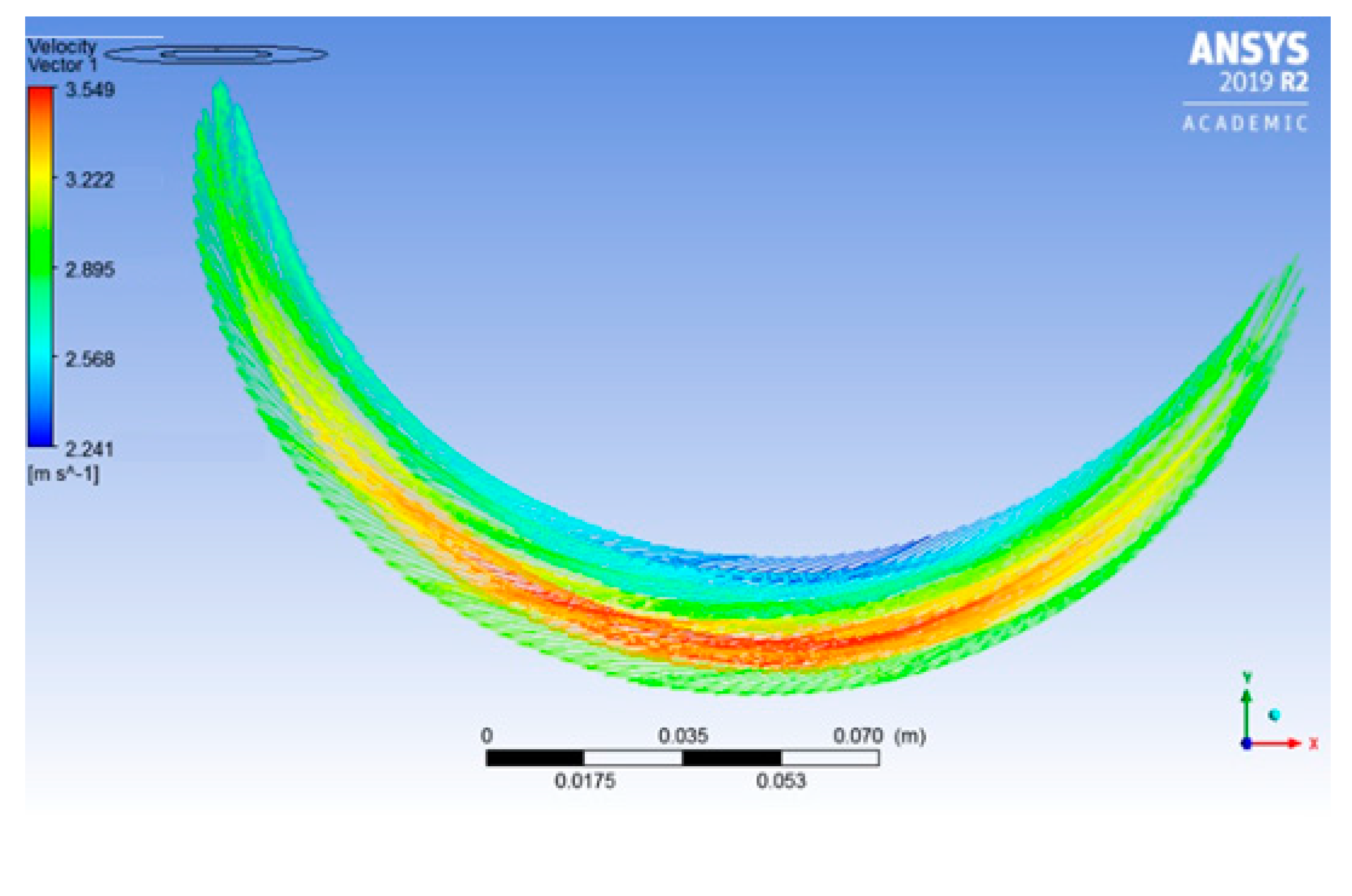
Prior to the construction of the model, it was assumed that bubble boiling occurs on the surface of the pipe in the boiler under consideration. Then the bubbles are transferred to the main stream. As the proportion of steam increases, a plug is formed, which can occupy the entire cross-section of the pipe, and therefore the flow rate increases significantly. At the same time, a boiling process can occur on the walls. This mode can be replaced by an annular one, when the pipe wall is covered with a film of liquid, and the central part is occupied by a steam-water mixture. According to the mathematical modeling and visualization obtained (an example of the movement of the coolant in the inner coil is shown in Figure 6), the velocity of the coolant reaches its maximum value in the center of the coil, which confirms the above hypothesis.

3.3. Recommendations for Calculating the Speed of the Steam-Water Mixture in Coils

Taking the volume flow rate of the m-th phase (20), m³/s:

$${\mathrm{Q}}_{\mathrm{m}}={\mathsf{\omega }}_{\mathrm{m}}\cdot \mathrm{S}=\frac{{\mathrm{V}}_{\mathrm{m}}}{\mathrm{t}}$$

(22)

where ${\mathsf{\omega }}_{\mathrm{m}}$—velocity of the heat carrier of the m-th phase, m/s; $\mathrm{S}$—the cross-sectional area of tubing, m²; ${\mathrm{V}}_{\mathrm{m}}$—the volume of the heat carrier of the m-th phase passing through the cross-section of the flow during time t, m³; $\mathrm{t}$—the time it takes for a liquid or vapor of volume ${\mathrm{V}}_{\mathrm{m}}$ to pass through the cross-section of the flow, s.

Therefore, the velocity of the coolant can be expressed in terms of Equation (23):

$${\mathsf{\omega }}_{\mathrm{m}}=\frac{{\mathrm{V}}_{\mathrm{m}}}{\mathrm{t}·\mathrm{S}}$$

(23)

However, it should be taken into account that the object in question has the shape of a coil consisting of pipelines of different diameters: the outer diameter of the coil is 28 mm, the inner diameter is 32 mm. In this regard need to be amended, taking into account the above changes and to take into account the diameter and height of the coaxial cylinders: 890 mm in the height and length of the outer coil respectively in 1680 mm and 172.95 m; inner coil—746 mm height 1664 mm and length 119.52 m.

The correction to the coolant velocity for each type of coil is presented in the expression (22):

$${\mathrm{z}}_{\mathrm{i}}=\frac{{\mathrm{H}}_{\mathrm{i}}·{\mathrm{d}}_{\mathrm{i}}}{{\mathrm{L}}_{\mathrm{i}}·{\mathrm{D}}_{\mathrm{i}}}$$

(24)

where ${\mathrm{H}}_{\mathrm{i}}$—the height of the coil, m; ${\mathrm{d}}_{\mathrm{i}}$—the diameter of the coil, m; ${\mathrm{L}}_{\mathrm{i}}$—coil length, m; ${\mathrm{D}}_{\mathrm{i}}$—diameter of the coaxial cylinder, m.

The calculation of the speed for the external coil, taking into account the expression (14) and the correction (22), is made according to Equation (23):

$${\mathsf{\omega }}_{\mathrm{m}}={\mathrm{z}}_{\mathrm{i}}{}^{0.52}·\frac{{\mathrm{V}}_{\mathrm{m}}}{\mathrm{t}·\mathrm{S}}$$

(25)

Calculation of the speed for the inner coil according to Equation (24):

$${\mathsf{\omega }}_{\mathrm{m}}={\mathrm{z}}_{\mathrm{i}}{}^{0.5}·\frac{{\mathrm{V}}_{\mathrm{m}}}{\mathrm{t}·\mathrm{S}}$$

(26)

4. Experimental Data

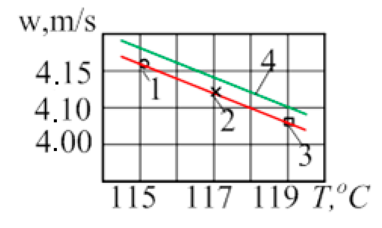
In December 2020, the authors tested a similar installation at an oil and gas field in the far north. The data obtained during these experiments agree very well with the calculated data, so the authors decided to present these data in

Table 2. The coolant velocity.

№	Temperature, °C	Speed (Experiment), m/s	Speed (Model), m/s
1	115	4.16	4.17
2	117	4.13	4.14
3	119	4.08	4.10

and Figure 7. The calculations for the coolant velocity based on experimental and theoretical calculations using mathematical modeling are presented in Table 2.

When constructing a mathematical model of the vaporization process, the theory of boiling and vaporization modes in coils was confirmed. However, the study showed that there is a high probability changes of the last mode dispersion when near a wall is formed a steam film, the conductivity decreases and the burnout of the tube wall, if not reduce the heat flux density applied to the coil. The amount of heat that is released into the environment in the presence of external and internal factors: poor quality of the coolant, intense combustion, wear of pipes, can serve as a catalyst and cause serious damage to the coils of the considered direct-flow boiler.

Mode 1. Experimental values of boiler operation 1 and 2, feed pumps 17, 18 and 21, 22, respectively, Figure 2 (

Table 3. Experimental values of Steam boiler 1.

Experiment	Measurements	Water Consumption	Water Temperature	Fuel Consumption	Steam Temperature after the Boiler	Steam Pressure after the Boiler
No.	No.	kg/s	°C	kg/s	°C	MPa
1	1	0.30944	44	0.01526	151	0.36
	2	0.33167	44	0.01517	151	0.36
	3	0.33361	44	0.01431	149	0.35
	4	0.34917	46	0.01558	151	0.36

and

Table 4. Experimental values of Steam boiler 2.

Experiment	Measurements	Water Consumption	Water Temperature	Fuel Consumption	Steam Temperature after the Boiler	Steam Pressure after the Boiler
No.	No.	kg/s	°C	kg/s	°C	MPa
2	1	0.37444	31	0.01866	159	0.49
	2	0.42389	26	0.01900	160	0.50
	3	0.43167	32	0.01873	159	0.49
	4	0.45750	32	0.01883	159	0.49

).

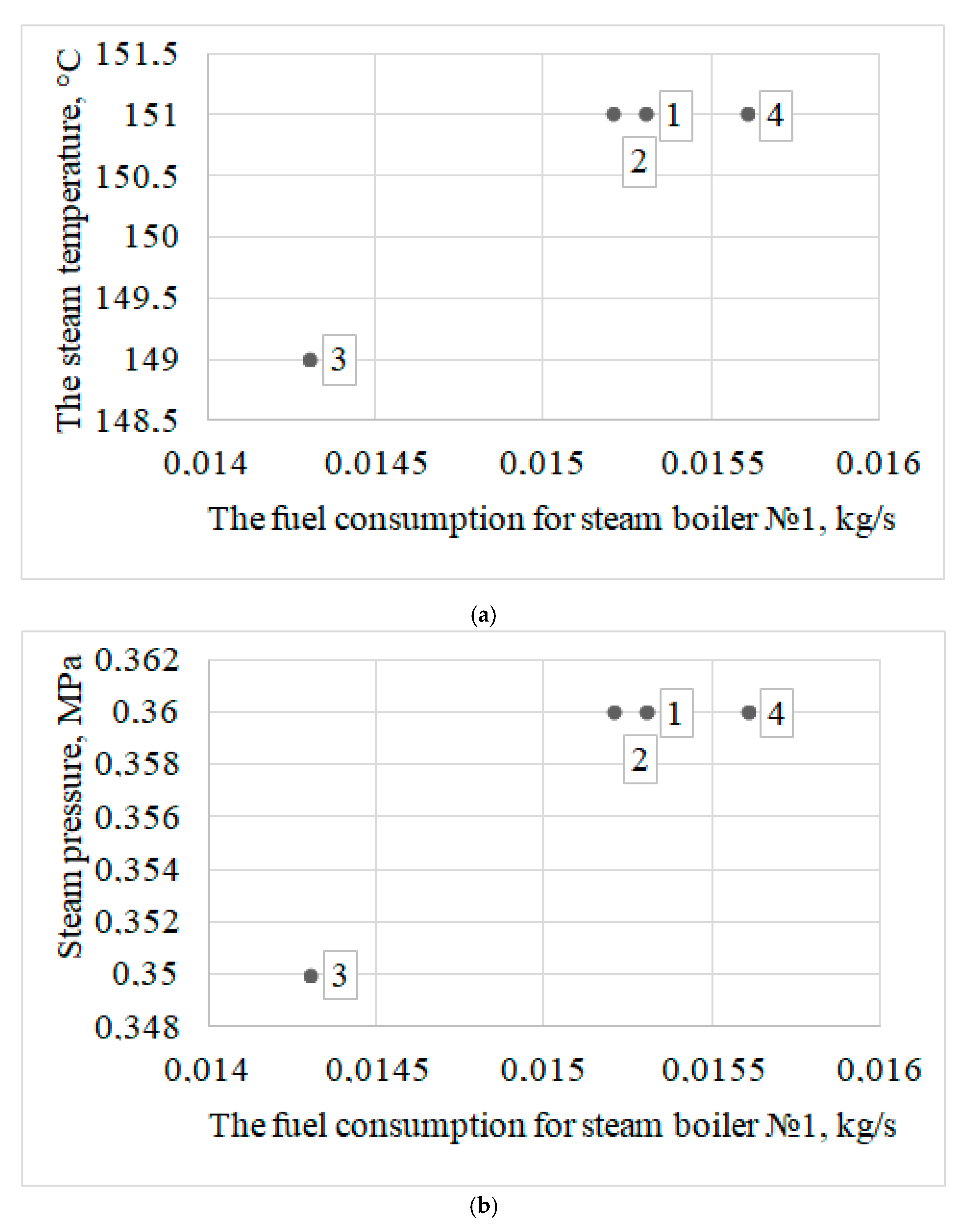
The correlation coefficient showing the relationship between the steam temperature and the fuel consumption for steam boiler No. 1 (Figure 8a) is 0.948, which indicates a strong relationship between these values. A positive correlation close to unity allows us to assert that an increase in one value affects the growth of the second, what is mentioned in the work of Pustylnik [30]. The correlation coefficient showing the relationship between the steam pressure and the fuel consumption of boiler No. 1 (Figure 8b) is also 0.948. A similar conclusion about the relationship between the steam temperature and the fuel consumption was taken to be valid for these values.

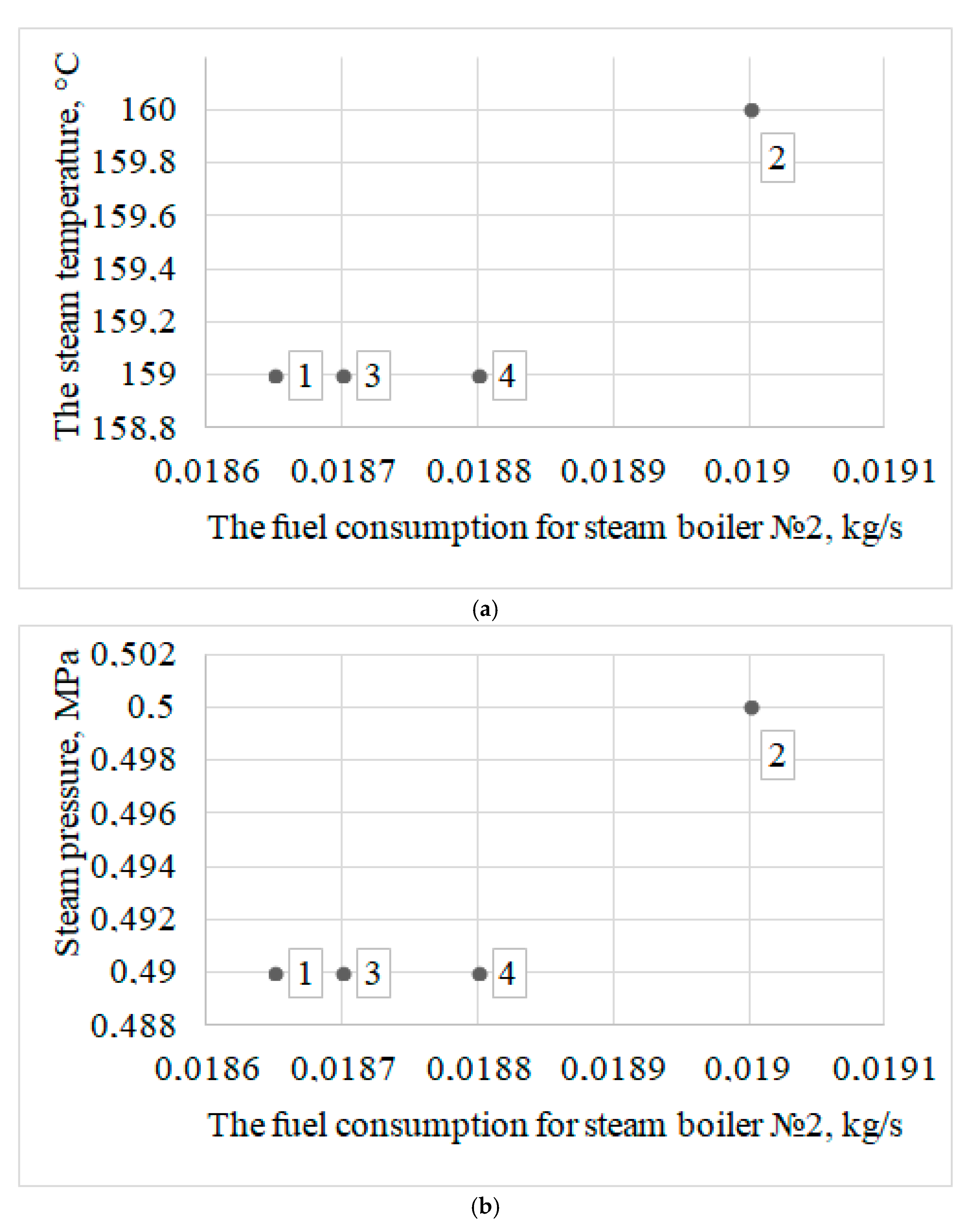
The correlation coefficient showing the relationship between the steam temperature and the fuel consumption for steam boiler No. 2 is 0.89, which indicates a sufficient relationship of these values. A positive correlation indicates that an increase in one value contributes to an increase in another, Figure 9.

The correlation coefficient showing the relationship between steam pressure and fuel consumption of boiler 2 is also 0.89. The above conclusion for the considered relationship between steam temperature and fuel consumption is also accepted for these parameters, Table 4.

Mode 2. Simultaneous operation of two boilers with the inclusion of two feed pumps,

Table 5. Experimental values of two steam boilers in mode 2.

Experiment	Measurements	Water Consumption	Water Temperature	Fuel Consumption	Steam Temperature after the Boiler	Steam Pressure after the Boiler
No.	No.	kg/s	°C	kg/s	°C	MPa
1	1	0.34278	45	0.01461	148	0.33
	2	0.34028	45	0.01449	156	0.43
	3	0.40194	53	0.01455	161	0.51
	4	0.35167	55	0.01487	160	0.49
2	1	0.38083	45	0.01983	152	0.36
	2	0.37167	45	0.01978	156	0.43
	3	0.33417	53	0.01988	160	0.49
	4	0.35611	55	0.01990	161	0.52

.

Both boilers and feed pumps are switched on to increase the steam output. All systems were working at full power. Table 5 shows the results of the experiment.

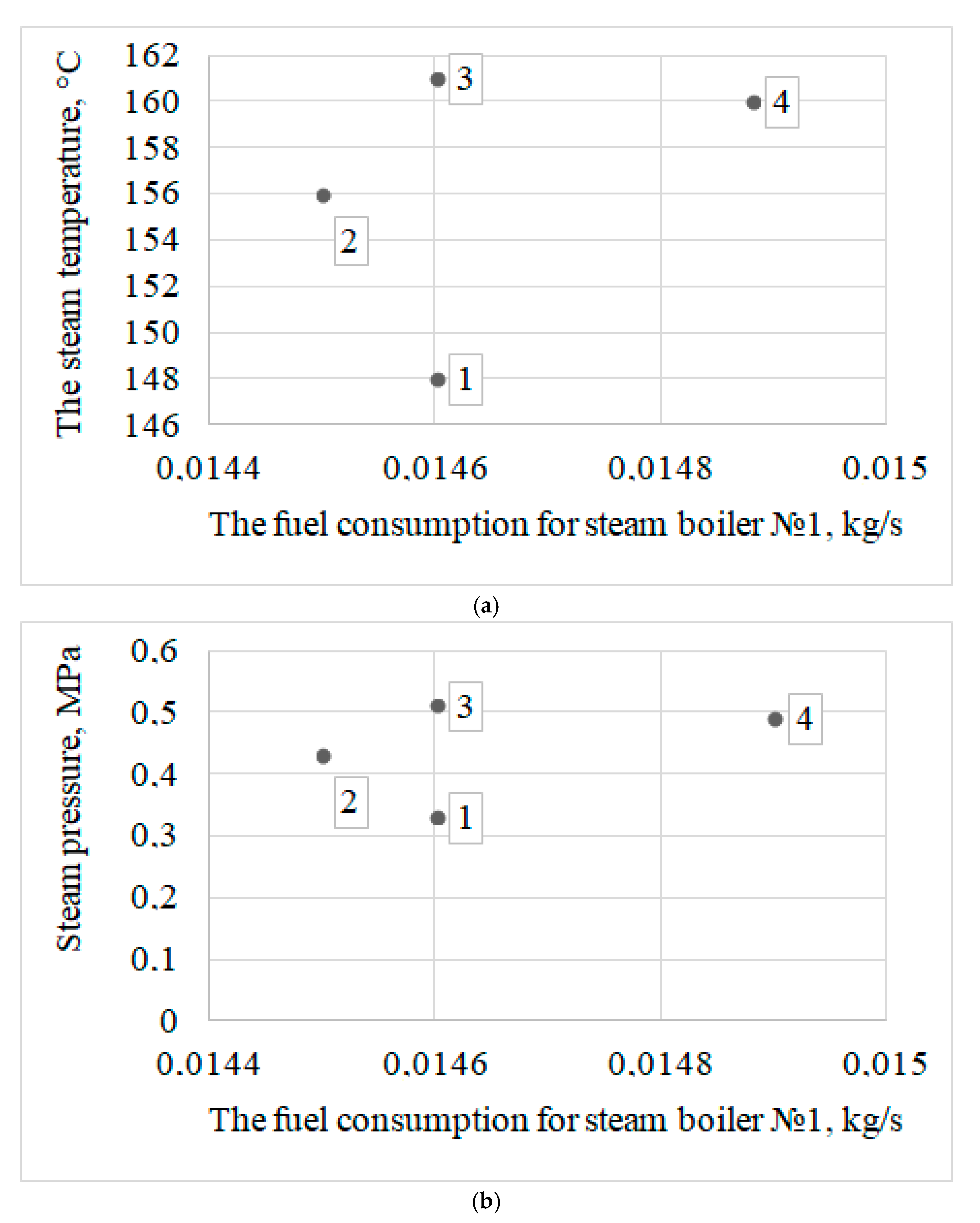
Figure 10 shows the relationship between temperature, steam pressure, and fuel consumption in the first boiler, respectively.

The correlation coefficient showing the relationship between steam temperature and fuel consumption, as well as the relationship between steam pressure and fuel consumption for steam boiler 1 in the second mode is 0.2306 and 0.2352, respectively. Points 1 and 3 illustrate that with a large difference in vapor pressure, the fuel consumption changed by a small value ΔB = 0.00006 kg/s. A small drop in fuel consumption is associated with a sharp increase in the temperature of the feed water, Δt = 8 °C (18). The increase in the temperature of the feed water reduced the boiler’s need for higher fuel consumption to maintain steam parameters (27):

$$\mathrm{B}=\frac{\mathrm{D}·\left({\mathrm{h}}^{″}-{\mathrm{h}}_{\mathrm{fw}}\right)}{\mathrm{NCV}·\mathsf{\eta }}·100,$$

(27)

where$\mathrm{B}$ is fuel consumption, kg/s; $\mathrm{D}$ is steam capacity, kg/s; ${\mathrm{h}}^{″},{ \mathrm{h}}_{\mathrm{fw}}$ is the enthalpy of steam and feed water, MJ/kg; $\mathrm{NCV}$ is net calorific value of fuel, MJ; $\mathsf{\eta }$ is boiler efficiency, %.

The experimental data also show that the feed water consumption at point 3 increased, which resulted in a sharp jump in all steam parameters at the boiler outlet. In connection with the analyzed corrections for the experimental values of temperature and feed water consumption, the smaller relationship between steam parameters and fuel consumption is explained.

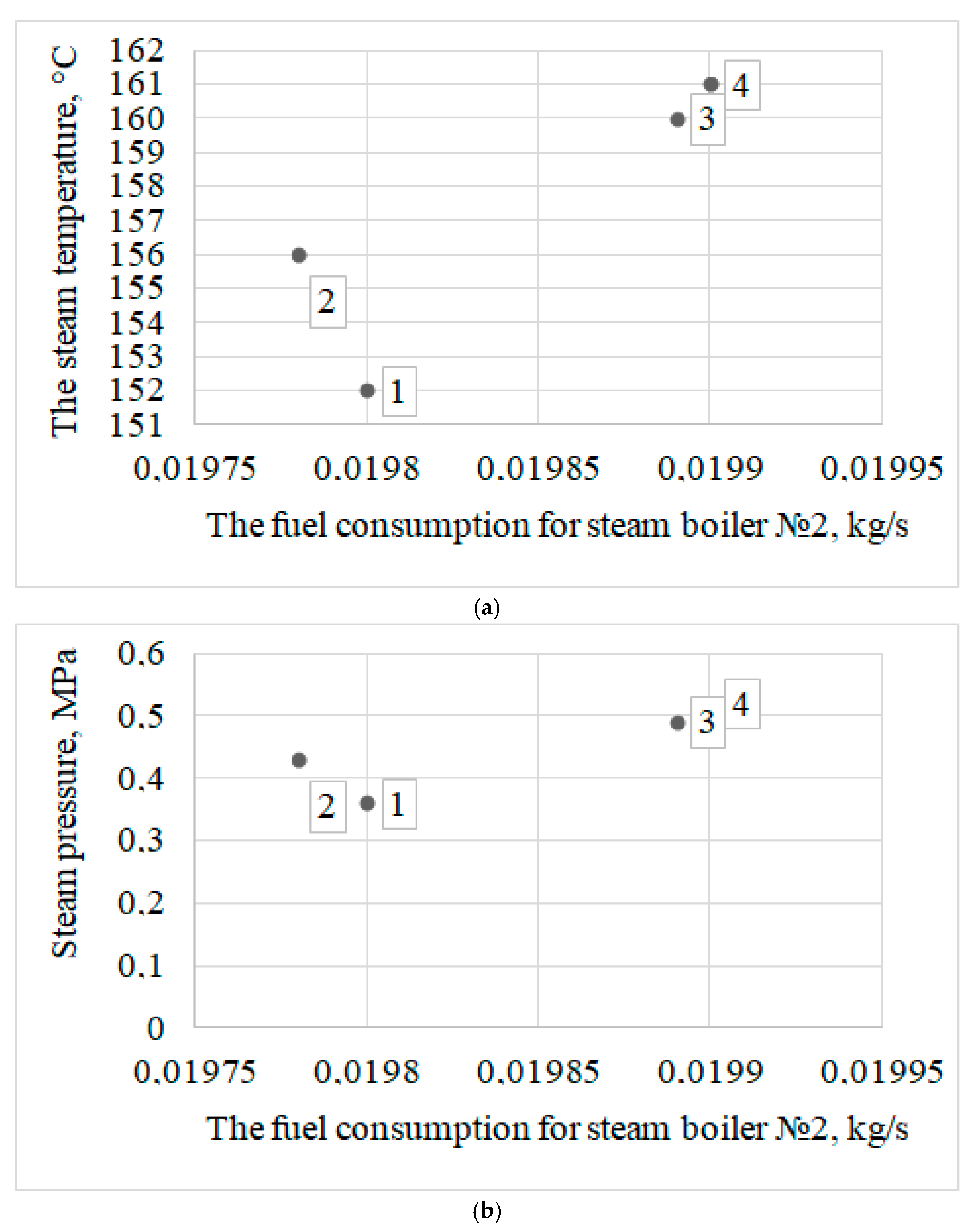
Figure 11 shows the relationship between temperature, steam pressure, and fuel consumption at the first boiler, respectively.

The correlation coefficient calculated to study the relationship between temperature, steam pressure, and fuel consumption on boiler 2 was 0.6895 and 0.6888, respectively. The experiment on the second boiler was carried out with a gradual increase in all parameters of the coolant; therefore, a stronger relationship is traced between temperature, steam pressure, and fuel consumption.

Thus, the analysis of the dependences of steam parameters and fuel consumption showed that the low storage capacity of once-through boilers is reflected in the temperature and pressure of the steam with changes in fuel consumption. Depending on the operating factors, the heating surface of the superheating zone changes. To maintain constant parameters of the coolant, it is necessary to maintain the ratio of the flow rate of feed water and fuel. In an earlier work, [31] the authors Osintsev et al. of the article proved a similar effect. In their work [31], the authors investigated a new design of a boiler unit that was part of an energy technology complex based on renewable energy sources. When conducting experimental tests, the authors proved that in direct-flow boilers, the working point (the ratio of parameters: temperature and pressure), at which the vaporization process begins, does not have a constant place (as it happens in boilers with drums), which in turn affects fuel consumption (you need to constantly monitor the flame). Therefore, the process is “floating”. With the help of graphs and calculations based on the data collected during the commissioning tests, the researchers were able to find a good ratio between fuel consumption and feed water to stabilize the boiler operation. The work described [31] was not only applied in nature, but in the patent for the invention, the authors were able to justify the efficiency of the boiler unit in “floating” modes.

Fuel consumption value is a dynamic characteristic for a once-through boiler. In a direct-flow boiler, the water–fuel ratio is regulated through the temperature and amount of feed water, by returning condensate, and installing a control valve. With low storage capacity, changes in the flow rate, quantity, and temperature of feed water affect the values ${\mathrm{D} \mathrm{and} \mathrm{h}}_{\mathrm{fw}}^{\prime }$, which affects the instantaneous change in the fuel consumption value $\mathrm{B}$.

Mode 3 (Table 3) for the first boiler and Mode 4 for the second are recorded in the performance-adjustment chart. In this mode, the outlet coolant is supplied with maximum parameters in terms of temperature and pressure at optimal fuel consumption for each boiler.

The coil-type boiler model has no drum. The vaporization process ends in a separator, which is installed outside the boiler. This has a positive effect on the quality of pipes during operation, deposits in the boiler elements form more slowly over time, thereby increasing the service life and reducing economic costs.

In their early works, the authors of the article presented the results of research on the operation of boiler units and heat and power equipment. For example, in [32] Toropov et al. presented new methods for studying the operation of boiler units, and in [33] E.V. Toropov et al. showed the possibility of organizing new methods in a new methodological framework. In addition, in [34], Toropov et al. proposed to use the results of [33] for low-and medium-pressure thermal power equipment. It should be noted that the paper by Osintsev et al. [35] shows the possibility of using the results of the work [33] in order to organize neural network control of combustion processes, including natural gas combustion. Thus, the methodological basis of the article was laid by the authors earlier in the work [33]. When introducing a new boiler unit to the drilling site, the operating company studied the thermal diagram of the entire production and the indicators of the coolant in each block. This examination confirmed the presence of heat losses to the environment on the lines and the absence of pressure gauges and thermometers. In addition, they confirmed that the connection of the pipelines did not provide the proper volume of the coolant when returning the condensate, which increased the consumption of make-up water. Analysis confirmed the need for modernization of the heating lines. Improvements to the scheme included changing the system of pipelines for returning condensate to the boiler room from the blocks, installing new instrumentation on the lines, insulating the pipelines, and installing an additional insulated tank for collecting condensate.

5. Empirical Coefficients Obtained from the Results of Experiments

The space formed by the coil cylinders and the wall of the boiler’s inner shell provides for the passage of flue gases. Two cylindrical boiler shells form an annular chamber for the passage of air from the fan to the burner device through the holes made in the base of the boiler [28]. Thus, heated air is supplied to the burner device, which increases the convective component of radiant-convective heat exchange in gas ducts (26):

$${\mathrm{Q}}_{\mathrm{f}}{=\mathsf{\alpha }}_{\mathrm{r}}·\mathrm{∆}{\mathrm{T}}_{\mathrm{gf}}·{\mathrm{F}}_1$$

(28)

where ${\mathsf{\alpha }}_{\mathrm{r}}$ is the heat transfer coefficient from the flame to the wall by radiation, W/(m²$·$K); $\mathrm{∆}{\mathrm{T}}_{\mathrm{gf}}$ is the temperature difference (27), $\mathrm{°}\mathrm{C}$; ${\mathrm{F}}_1$ is the internal surface area of the furnace, m²:

$$\mathrm{∆}{\mathrm{T}}_{\mathrm{gf}}={\mathrm{T}}_{\mathrm{gas}}^{\prime }-{\mathrm{T}}_{\mathrm{w}1},$$

(29)

where ${\mathrm{T}}_{\mathrm{gas}}^{\prime }$ is characteristic temperature of the gas-air flow (28), $\mathrm{°}\mathrm{C}$; ${\mathrm{T}}_{\mathrm{w}1}$ is the average temperature of the furnace wall, $\mathrm{°}\mathrm{C}$:

$${\mathrm{T}}_{\mathrm{gas}}^{\prime }={\mathrm{T}}_{\mathrm{air}}+{\mathrm{c}}_{\mathrm{t}}·\left({\mathrm{T}}_{\mathrm{gas}}-{\mathrm{T}}_{\mathrm{air}}\right),$$

(30)

where ${\mathrm{T}}_{\mathrm{air}}$ is the air temperature, $\mathrm{°}\mathrm{C}$; ${\mathrm{c}}_{\mathrm{t}}$ is the temperature correction; ${\mathrm{T}}_{\mathrm{gas}}$ is the gas temperature, $\mathrm{°}\mathrm{C}$.

Let us compare our test results with the calculated values. Processing the experimental results guides the changes to be made to technical and economic parameters of the boiler and the practical assessment of the presented coil design. When comparing the experimental and calculated results, correction factors were introduced while adhering to the equality of the initial parameters (29). The equality of the initial parameters is based on losses ${\mathrm{q}}_2$, since this parameter is affected by changes within the known limits of the initial input values of the defining quantities:

$${\mathrm{q}}_2^{\mathrm{l}}={\mathrm{q}}_2\pm \mathrm{∆}{\mathrm{q}}_2^{\mathrm{c}.\mathrm{air}}\pm \mathrm{∆}{\mathrm{q}}_2^{\mathrm{a}.\mathrm{h}}\pm \sum {\mathrm{k}}_{\mathrm{t}}\mathrm{∆}\mathrm{m},$$

(31)

where ${\mathrm{q}}_2$ is the heat loss with exhaust gases, %; $\mathrm{∆}{\mathrm{q}}_{\mathrm{2}}^{\mathrm{c}.\mathrm{a}\mathrm{i}\mathrm{r}}$ is the correction for deviation of cold air temperature (30); $\mathrm{∆}{\mathrm{q}}_2^{\mathrm{a}.\mathrm{h}}$ is the change in ${\mathrm{q}}_2$ values when heating air in the air heater by $\mathrm{∆}{\mathrm{T}}_{\mathrm{gf}}$ (31); $\mathrm{\sum }{\mathrm{k}}_{\mathrm{t}}\mathrm{∆}\mathrm{m}$ is the sum of the products of the correction factors for the deviation of the initial parameter by ∆m, nominal or calculated:

$$\mathrm{∆}{\mathrm{q}}_2^{\mathrm{c}.\mathrm{air}}={\mathrm{q}}_2·\frac{{\mathrm{t}}_{\mathrm{c}.\mathrm{air}}^{\mathrm{calc}}-{\mathrm{t}}_{\mathrm{c}.\mathrm{air}}^{\exp }}{{\vartheta }_{\mathrm{ex}}-{\mathrm{t}}_{\mathrm{c}.\mathrm{air}}^{\exp }}$$

(32)

where ${\mathrm{t}}_{\mathrm{c}\mathrm{.}\mathrm{a}\mathrm{i}\mathrm{r}}^{\mathrm{c}\mathrm{a}\mathrm{l}\mathrm{c}}$ is the cold air temperature, calculated, °C; ${\mathrm{t}}_{\mathrm{c}\mathrm{.}\mathrm{a}\mathrm{i}\mathrm{r}}^{\mathrm{e}\mathrm{x}\mathrm{p}}$ is the cold air temperature, experimental value, °C; ${\vartheta }_{\mathrm{e}\mathrm{x}}$ is the flue gas temperature, °C:

$$\mathrm{∆}{\mathrm{q}}_2^{\mathrm{a}.\mathrm{h}}={\mathrm{k}}_{\mathrm{a}.\mathrm{h}} ·\left({\mathrm{t}}_{\mathrm{a}.\mathrm{h}}^{\mathrm{calc}}-{\mathrm{t}}_{\mathrm{a}.\mathrm{h}}^{\exp }\right)$$

(33)

where ${\mathrm{t}}_{\mathrm{a}\mathrm{.}\mathrm{h}}^{\mathrm{c}\mathrm{a}\mathrm{l}\mathrm{c}}$ is the air temperature after the air heater, calculated, °C; ${\mathrm{t}}_{\mathrm{a}\mathrm{.}\mathrm{h}}^{\mathrm{e}\mathrm{x}\mathrm{p}}$ is the air temperature after the air heater, experimental value, °C, ${\mathrm{k}}_{\mathrm{a}\mathrm{.}\mathrm{h}}$ is the correction factor.

Consequently, by comparing the calculated and empirically-obtained temperatures, the coefficient ${\mathrm{c}}_{\mathrm{w}}$, was introduced, which summarizes the correction factors used in deviations for the cold air temperature and after the air heater. Thus, equation has been improved in terms of introducing correction factors for flow turbulization and for the variable value of the equivalent diameter of annular channels formed by coaxial cylindrical surfaces of the coils (32) and for a change in air temperature after the air heater (33).

$${\mathrm{c}}_{\mathrm{f}}={\left(\frac{{\mathrm{D}}_2}{{\mathrm{D}}_1}\right)}^{0.5},$$

(34)

$${\mathrm{c}}_{\mathrm{w}}={\left(1+\mathrm{∆}{\mathrm{T}}^{\left(-0.5\right)}\right)}^{0.25}.$$

(35)

Taking into account the correction factors, equation is transformed (36):

$${\mathrm{Q}}_{\mathrm{f}}={\mathrm{c}}_{\mathrm{f}}·{\mathrm{c}}_{\mathrm{w}}·{\mathsf{\alpha }}_{\mathrm{r}}·\mathrm{∆}{\mathrm{T}}_{\mathrm{gf}}·{\mathrm{F}}_1$$

(36)

Experimental coefficients (32) and (33) were obtained for the first time, used in the thermal calculation of the boiler in Equation (34) taking into account the normative methodology.

6. Results and Discussion

Based on formulas specified above, the dependences of the coefficient ${\mathrm{c}}_{\mathrm{w}}$ on ${\mathrm{T}}_{\mathrm{c}.\mathrm{a}}$ and ${\mathrm{T}}_{\mathrm{h}.\mathrm{a}}$ for a coil-type steam boiler are obtained (

Table 6. Dependency of the coefficient ${\mathrm{c}}_{\mathrm{w}}$ on the temperatures of cold and heated air for a coil-type steam boiler.

	With the Coldest Five Days, °C	At the Average Temperature of the Coldest Month, °C	At the Air Temperature t = +8 °C
${\mathrm{T}}_{\mathrm{c}.\mathrm{a}}$, $\mathrm{°}$C	−40	−25	+8
${\mathrm{T}}_{\mathrm{h}.\mathrm{a}}$, $\mathrm{°}$C	+27	+58	+65
${\mathrm{c}}_{\mathrm{w}}$	1.029	1.026	1.032

For the coefficient ${\mathrm{c}}_{\mathrm{w}}$ the equation of the normal probability density distribution is as follows.

and Figure 12). The data in Table 6 can be used for structural and verification calculations.

At the same time for ${\mathrm{c}}_{\mathrm{w}}$ Similarly, we get the band of uncertainty: the lower bound is 1.024, the upper bound is 1.034. The authors would like to note that during the experiment, the values ΔT for the coefficient ${\mathrm{c}}_{\mathrm{w}}$ were studied from the obtained data, based on the sample. The values ΔT obtained include the effects of influence from external factors, the overall standard deviation was estimated, and a sensitivity analysis was performed.

Mikhaylenko’s recent research shows that the theory of heat and mass transfer, in particular the flow of gases and liquids, has its drawbacks in relation to experimental studies of boiler installations. Mikhaylenko presented the results of the research in the form of a developed model [36]. Bruce-Konuah et al. [17] proposed a hypothesis for the behavior of the air flow on a weakly isothermal model, as well as for computer modeling of the movement of heated gases, and this hypothesis was partially confirmed by the developed mathematical model, which is consistent with the results of the studies of Sweetnam et al. [6]. The hypotheses considered in the review were confirmed by the construction of mathematical models. These models fully correspond to each other, as well as to the basic physical laws, in particular, the equations of conservation of mass and energy, as well as the boundary conditions of heat exchange and gas dynamic processes.

In the works of Hameed et al. [37] and Boje [38], the authors propose mathematical models that are applicable to the hydro-and gas dynamics of boiler units of similar designs.

In Trojan [39], the author proposes a non-standard mathematical model applicable to a steam generator. In [40], Orlov et al. propose a whole software package for calculating the hydrodynamics of a boiler unit.

All these works have their disadvantages and advantages. At the same time, since the boiler unit considered in this article is unique, it is difficult to make an exact match based on the results of scientific analysis of developments and models. The authors of this article, in fact, develop specific mathematical models that are applicable for a new type of steam generators.

Let’s compare the data obtained by different authors, for example, on the hydrodynamics of water in a boiler unit (

Table 7. Comparison of the authors’ experimental data and simulation results [40] at the temperature of 120 °C.

Parameter	Speed (Experiment), m/s	Speed (Model), m/s	Speed (Experiment), m/s [40]	Speed (Model), m/s [40]
temperature of 120 °C	4.06	4.08	4.07	4.06

and

Table 8. Comparison of the authors’ experimental data and simulation results [15,16] at the temperature of 115 °C.

Parameter	Speed (Experiment), m/s [15]	Speed (Model), m/s [15]	Speed (Experiment), m/s [16]	Speed (Model), m/s [16]
temperature of 115 °C	4.16	4.18	4.21	4.20

).

Let us compare the same data with the results of hydrodynamic modeling presented in the works of Bag [15] and an article by Buck [16].

7. Conclusions

Coil-type steam boilers have withstood operation at the oil field “Var-Yogan” in the subarctic continental climate as part of a modernized boiler plant.

The results of our analysis of the experimental data collected from the MTPB in real working conditions allow us to draw the following particular conclusions that are of interest to this experimental theoretical study:

(1)

We introduce correction factors for the equation of the convective component of radiant-convective heat transfer in the gas ducts. With these correction factors, ${\mathrm{Q}}_{\mathrm{f}}$ is close to the real value, taking into account the design features of the boiler. The results of the dependence of the correction factor ${\mathrm{c}}_{\mathrm{w}}$ on the temperature of the outside and heated air are presented. During experimental operation, the advantages of the compact design of the boilers were proven.

(2)

Testing the boiler plant showed that a stable fuel temperature provided the required viscosity and good fuel atomization. Along with the change in the consumption of feed water and fuel, there was a significant change in temperature and steam pressure due to the low storage capacity of the once-through boilers. Losses with underburning and outgoing heat have decreased.

(3)

A methodological basis for analytical and experimental studies of radiation and convective heat transfer in a direct-flow steam generator of the coil type has been developed.

(4)

For the first time, experimental coefficients have been obtained that can be used for direct-flow steam generators of the coil type, which will increase the efficiency of these heat exchange devices.

(5)

The experimental data underwent sensitivity analysis, including an uncertainty band, and the methodology was validated. Data from experiments and simulations are compared with the results of other authors.

References

- Arnfield, A.J. Köppen Climate Classification; Encyclopædia Britannica, Inc.: Chicago, IL, USA, 2020; Available online: https://www.britannica.com/science/Koppen-climateclassification (accessed on 11 December 2020).
- Chen, D.; Chen, H.W. Using the Köppen classification to quantify climate variation and change: An example for 1901–2010. Environ. Dev. 2013, 6, 69–79. [Google Scholar] [CrossRef]
- Mazzeo, D.; Matera, N.; De Luca, P.; Baglivo, C.; Congedo, P.M.; Oliveti, G. Worldwide geographical mapping and optimization of stand-alone and grid-connected hybrid renewable system techno-economic performance across Köppen-Geiger climates. Appl. Energy 2020, 276, 115507. [Google Scholar] [CrossRef]
- Bennett, G.J. The Secret Life of Boilers: Dynamic Performance of Residential Gas Boiler Heating Systems—A Modelling and Empirical Study. In Proceedings of the CIBSE Technical Symposium, Sheffield, UK, 25–26 April 2019; pp. 25–26. [Google Scholar]
- Bennett, G.; Elwell, C.; Oreszczyn, T. Space heating operation of combination boilers in the UK: The case for addressing real-world boiler performance. Build. Serv. Eng. Res. Technol. 2019, 40, 75–92. [Google Scholar] [CrossRef] [Green Version]
- Sweetnam, T.; Spataru, C.; Barrett, M.; Carter, E. Domestic demand-side response on district heating networks. Build. Res. Inf. 2018, 47, 330–343. [Google Scholar] [CrossRef] [Green Version]
- Hernández Corona, J.L.; Vázquez, E.M.; Sánchez Lima, H.V.; Fragoso Parra, G.A.; Espinoza Peralta, J.A. Steam Generator for External Resistances. J. Sci. Res. Publ. 2020, 10, 463–469. [Google Scholar] [CrossRef]
- Guidez, J.; Prele, G. The Steam Generators. In Superphenix; Atlantis Press: Paris, France, 2017; p. 130. [Google Scholar]
- Sharma, A.; Sharma, M.; Shukla, A.K.; Negi, N. Evaluation of Heat Recovery Steam Generator for Gas/Steam Combined Cycle Power Plants. In Advances in Fluid and Thermal Engineering; Lecture Notes in Mechanical Engineering; Saha, P., Subbarao, P., Sikarwar, B., Eds.; Springer: Singapore, 2019. [Google Scholar] [CrossRef]
- Astorga-Zaragoza, C.-M.; Osorio-Gordillo, G.-L.; Reyes-Martínez, J.; Madrigal-Espinosa, G.; Chadli, M. Takagi—Sugeno Observers as an Alternative to Nonlinear Observers for Analytical Redundancy. Application to a Steam Generator of a Thermal Power Plant. Int. J. Fuzzy Syst. 2018, 20, 1756–1766. [Google Scholar] [CrossRef]
- Silva, P.R.S.; Leiroz, A.J.K.; Cruz, M.E.C. Evaluation of the efficiency of a heat recovery steam generator via computational simulations of off-design operation. J. Braz. Soc. Mech. Sci. Eng. 2020, 42, 1–18. [Google Scholar] [CrossRef]
- Cheridi, A.L.D.; Loubar, A.; Dadda, A.; Bouam, A. Modeling and simulation of a natural circulation water-tube steam boiler. SN Appl. Sci. 2019, 1, 1405. [Google Scholar] [CrossRef] [Green Version]
- Moghari, M.; Hosseini, S.; Shokouhmand, H.; Sharifi, H.; Izadpanah, S. A numerical study on thermal behavior of a D-type water-cooled steam boiler. Appl. Therm. Eng. 2012, 37, 360–372. [Google Scholar] [CrossRef]
- Sunil, P.U.; Barve, J.; Nataraj, P.S.V. Mathematical modeling, simulation and validation of a boiler drum: Some investigations. Energy 2017, 126, 312–325. [Google Scholar] [CrossRef]
- Hag, E.E.; Rahman, T.U.; Ahad, A.; Ali, F.; Ijaz, M. Modeling and simulation of an industrial steam boiler. Int. J. Comput. Eng. Inf. Technol. 2016, 8, 7–10. [Google Scholar]
- Backi, C.J. Nonlinear modeling and control for an evaporator unit. Control Eng. Pract. 2018, 78, 24–34. [Google Scholar] [CrossRef]
- Bruce-Konuah, A.; Jones, R.V.; Fuertes, A.; De Wilde, P. Central heating settings in low energy social housing in the United Kingdom. Energy Procedia 2019, 158, 3399–3404. [Google Scholar] [CrossRef]
- Dixon, D.; Nguyen, A. An Empirical Oil, Steam, and Produced-Water Forecasting Model for Steam-Assisted Gravity Drainage with Linear Steam-Chamber Geometry. SPE Reserv. Evaluation Eng. 2019, 22, 1615–1629. [Google Scholar] [CrossRef]
- Kusumastuti, I.; Erfando, T.; Hidayat, F. Effects of Various Steam Flooding Injection Patterns and Steam Quality to Recovery Factor. J. Earth Energy Eng. 2019, 8, 33–39. [Google Scholar] [CrossRef]
- Badur, J.; Bryk, M. Accelerated start-up of the steam turbine by means of controlled cooling steam injection. Energy 2019, 173, 1242–1255. [Google Scholar] [CrossRef]
- Duarte, C.A.; Espejo, E.; Martinez, J.C. Failure analysis of the wall tubes of a water-tube boiler. Eng. Fail. Anal. 2017, 79, 704–713. [Google Scholar] [CrossRef]
- Chauhan, S.S.; Khanam, S. Energy integration in boiler section of thermal power plant. J. Clean. Prod. 2018, 202, 601–615. [Google Scholar] [CrossRef]
- Shi, Y.; Wang, J. Ash fouling monitoring and key variables analysis for coal fired power plant boiler. Therm. Sci. 2015, 19, 253–265. [Google Scholar] [CrossRef]
- Kuznetsov, N.V. Direct-flow two-stage steam generator: Pat. RU89623U1. Ros. Federation No. 2009130968/22. In Thermal Calculation of Boiler Units: Standard Method; Kuznetsov, N.V., Mitor, V.V., Dubrovsky, I.E., Eds.; EKOLIT: Moscow, Russia, 2011; 296p. (In Russian) [Google Scholar]
- Lummi, A.P. Calculation of a Hot Water Boiler; Lummi, A.P., Munts, V.A., Eds.; GOU VPO USTU-UPI: Yekaterinburg, Russia, 2009; 41p. (In Russian) [Google Scholar]
- Sidelkovsky, L.N. Boiler Plants for Industrial Enterprises. Textbook for Universities in the Specialty "Industrial Heat Power", 4th ed.; Sidelkovsky, L.N., Yurenev, V.N., Eds.; Moscow Bastet: Moscow, Russia, 2009; 526p. (In Russian) [Google Scholar]
- Trembovlya, V.I. Heat Engineering Tests of Boiler Plants, 2nd ed.; Trembovlya, V.I., Finger, E.D., Avdeeva, A.A., Eds.; Energoatomizdat: Moscow, Russia, 1991; 416p. (In Russian) [Google Scholar]
- Zykov, A.K. Steam and Hot Water Boilers: Reference Book, 2nd ed.; Zykov, A.K., Ed.; NPOOBT: Moscow, Russia, 1995; 119p. (In Russian) [Google Scholar]
- Lipov, Y.M. Layout and Thermal Calculation of a Steam Boiler: Textbook for Universities; Lipov, Y.M., Samoilov, Y.F., Vilensky, T.V., Eds.; Energoatomizdat: Moscow, Russia, 1988; 208p. (In Russian) [Google Scholar]
- Pustylnik, E.I. Statistical Methods of Analysis and Processing of Observations; Nauka: Moscow, Russia, 1968; 288p. [Google Scholar]
- Osintsev, K.V.; Osintsev, V.V.; Bogatkin, V.I.; Toropov, E.V.; Kuskarbekova, S.I. Liquid Electric Heater. Patent 2694890, 18 July 2019. [Google Scholar]
- Toropov, E.V.; Osintsev, K.V.; Aliukov, S.V. Analysis of the calculated and experimental dependencies of the combustion of coal dust on the basis of a new methodological base of theoretical studies of heat exchange processes. Int. J. Heat Technol. 2018, 36, 1240–1248. [Google Scholar] [CrossRef]
- Toropov, E.; Osintsev, K.; Aliukov, S. New Theoretical and Methodological Approaches to the Study of Heat Transfer in Coal Dust Combustion. Energies 2019, 12, 136. [Google Scholar] [CrossRef] [Green Version]
- Alabugin, A.; Aliukov, S.; Osintsev, K. Combined Approach to Analysis and Regulation of Thermodynamic Processes in the Energy Technology Complex. Process 2021, 9, 204. [Google Scholar] [CrossRef]
- Osintsev, K.; Aliukov, S.; Prikhodko, Y. New Methods for Control System Signal Sampling in Neural Networks of Power Facilities. IEEE Access 2020, 8, 1. [Google Scholar] [CrossRef]
- Mikhaylenko, E.V. How to improve the characteristics of mobile generators. Chief Power Eng. 2015, 5–6, 65–71. (In Russian) [Google Scholar]
- Hameed, V.; Fatima, J.H. Investigation study of vertical helical coil heat exchanger. In Proceedings of the 2nd International Conference on Materials Engineering & Science, Baghdad, Iraq, 25–26 September 2020; Volume 2213. [Google Scholar]
- Boje, E. Dry-out point estimation in once through boilers. IFAC Proc. Vol. 2009, 42, 723–728. [Google Scholar] [CrossRef]
- Trojan, M. Modeling of a steam boiler operation using the boiler nonlinear mathematical model. Energy 2019, 175, 1194–1208. [Google Scholar]
- Orlov, K.A. Program complex “WaterSteamPro” for calculating the thermophysical properties of water and water vapor. In Proceedings of the X Russian Conference on Thermophysical Properties of Substances: Abstracts of Reports, Moscow, Russia, 15–19 October 2018; Orlov, K.A., Alexandrov, A.A., Ochkov, V.F., Ochkov, A.V., Eds.; Publishing House “Butlerov Communications”: Kazan, Russia, 2002; pp. 187–188. (In Russian). [Google Scholar]
Figure 1.
Coil-type steam boiler.
Figure 2.
Schematic of the MTPB: (1, 2) steam boiler; (3) reserve fuel tank; (4) chemical water treatment unit; (5) nutritional container; (6) distribution manifold; (7–9) valve (steam to the consumer); (10) valve (steam for own needs); (11) valve (steam for heating the tank); (12, 13) valve; (14, 15) relief safety valve; (16, 20) check valve; (17, 18, 21, 22) feed pump; (19, 23, 24, 27, 28, 30, 31, 34, 35, 37–39) valve; (25, 32) separator; (26, 33) fine filter; (29, 36) coarse filter; (40) pump.
Figure 3.
Validation error (Normal).
Figure 4.
Validation error (Lognormal).
Figure 5.
Coaxial cylinders consisting of spiral coils.
Figure 6.
Model of the steam formation process in the coil of a direct-flow steam boiler.
Figure 7.
Changing the speed of the coolant at different temperatures: 1, 2, 3-speed data, taking into account the uncertainty, obtained when 115, 117, 119 °C, 4-simulation data.
Figure 8.
Relationship between parameters in Steam boiler 1: (a) relationship between steam temperature and fuel consumption, (b) relationship between steam pressure and fuel.
Figure 9.
Relationship between parameters in Steam boiler 2: (a) relationship between steam temperature and fuel consumption, (b) relationship between steam pressure and fuel.
Figure 10.
Figure 11.
Figure 12.
Normal distribution of the probability density of the coefficient : (a) lognormal, (b) normal, σ—standard deviation (3 values are sufficient σ to construct the law of normal distribution, the values of σ selected for each specific case in Matlab).