Computational Fluid Dynamics Simulations for Investigation of the Damage Causes in Safety Elements of Powered Roof Supports—A Case Study

Abstract

The paper describes a case study of the safety hydraulic system damage in the working of a longwall in a Polish coal mine. The safety elements are a component of the powered roof supports which secure the shield against damage during rock burst incidents. The damage event, which occurred in the hydraulic system during the mining process, caused the uncontrolled lowering of the powered roof support height during the mining process. The uncontrolled lowering of a shield may cause the danger of the loss of the stability along the longwall working in the form of a rock burst and collapses and may represent a serious and immediate danger to the safety and health of employees. Based on the results of the computational fluid dynamics methods (CFD) analysis of the safety elements in the hydraulic system of longwall 2-leg shield, the causes of damage were diagnosed and presented. The CFD and the strength analysis by the finite element method (FEM) were used for numerical modeling. The diagrams and maps of changes of parameters having an impact on the damage mechanism in safety elements of the hydraulic leg were developed based on the results of model tests. The forecasted values of stress distributions in the safety system of the hydraulic leg have made it possible to identify the reasons of the damage causes, verified by real observations.

1. Introduction

According to the 2020 annual report on the state of basic natural and technical hazards in the conditions of Polish mining [1], total extraction from regions classified as threatened by rock bursts amounted to approximately 54% of the total production volume. Since classifying the coal seam or part of it to the appropriate degree of rock burst hazard is not a measure of the occurrence or not of a high-energy rock tremor, and it should be assumed that rock mass tremors currently affect over 60% of the exploited coal seams and show a growing tendency (due to deteriorating geological and mining conditions associated with increasing cover depth, and the occurrence of exploitation problems).

Pursuant to the requirements of the Health and Safety Ministry [2], powered supports intended for use in conditions with a risk of rock mass tremors should be adapted to absorb dynamic loads. The assessment and guidelines are prepared by the Central Mining Institute (GIG) according to its own method for selecting shields for mining conditions. The GIG method is an analytical method, which is widely used in mining practice, using the technical parameters of the powered roof support and many years of experience.

The main goal of the method is to determine the safe scope of its work for the considered case of the powered roof support [3]. The method takes into account the fluid flow in the safety elements of the powered roof support which secure the hydraulic legs against overloads [4]. The safety elements of the powered roof support consist of a pressure-limiting hydraulic valve and a connection pipe supplying fluid from the hydraulic legs to the valve [5,6,7]. The characteristics of liquid flow in safety elements, which are understood as the dependence of pressure on the volumetric fluid flow together with the parameters of the hydraulic valve, determine the effectiveness of the safety elements of the powered roof support against its overload [8]. The extraction of the coal seams at greater depth and the real risk of rock mass tremors, requires the use of hydraulic legs with increasingly large bearing capacities. The introduction of shields with a piston diameter of the hydraulic leg above Ø 0.32 m into operation and additionally hydraulic legs with a drilled cylinder shell (an outlet for fluid from the working space under the piston of the hydraulic leg), has resulted in the appearance of phenomena not previously observed in modern shields, i.e. hydraulic shocks (fluid hammer) causing the excitation of the safety system. According to [9], hydraulic shocks are the phenomenon of strong pressure oscillations in a pipe operating under pressure, caused by rapid changes in the velocity of the fluid flow in a short time. The hydraulic shocks in the safety elements of a hydraulic leg are characterized by vibration frequencies of several hundred Hertz (Hz) and amplitudes significantly exceeding the operating values. The effect of the hydraulic shocks is a loss of tightness in the safety elements of the powered roof support, and reduction or loss of the load bearing capacity of the powered roof support, which consequently may lead to the uncontrolled lowering of the shield height [10,11,12,13,14].

Identification of the aforementioned hazards and their elimination is a significant problem for the efficiency of mining processes and work safety [15,16]. Therefore, this paper attempts to describe the causes of damage events occurring in a working overflow valve during the mining process based on the results of the numerical simulations using the CFD and FEM methods.

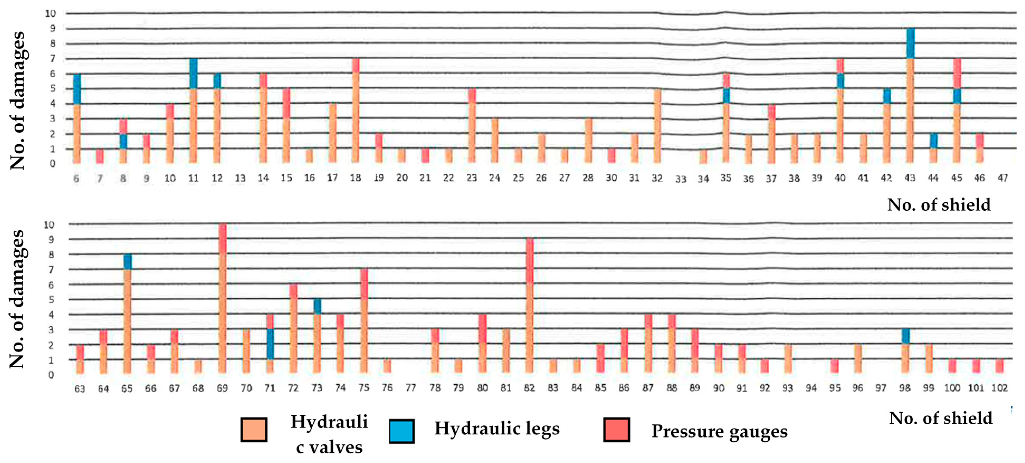
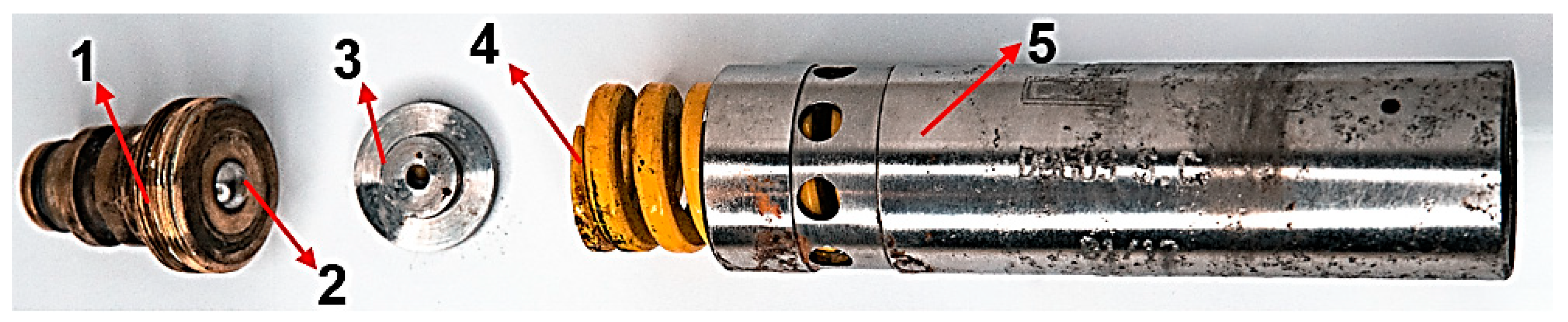
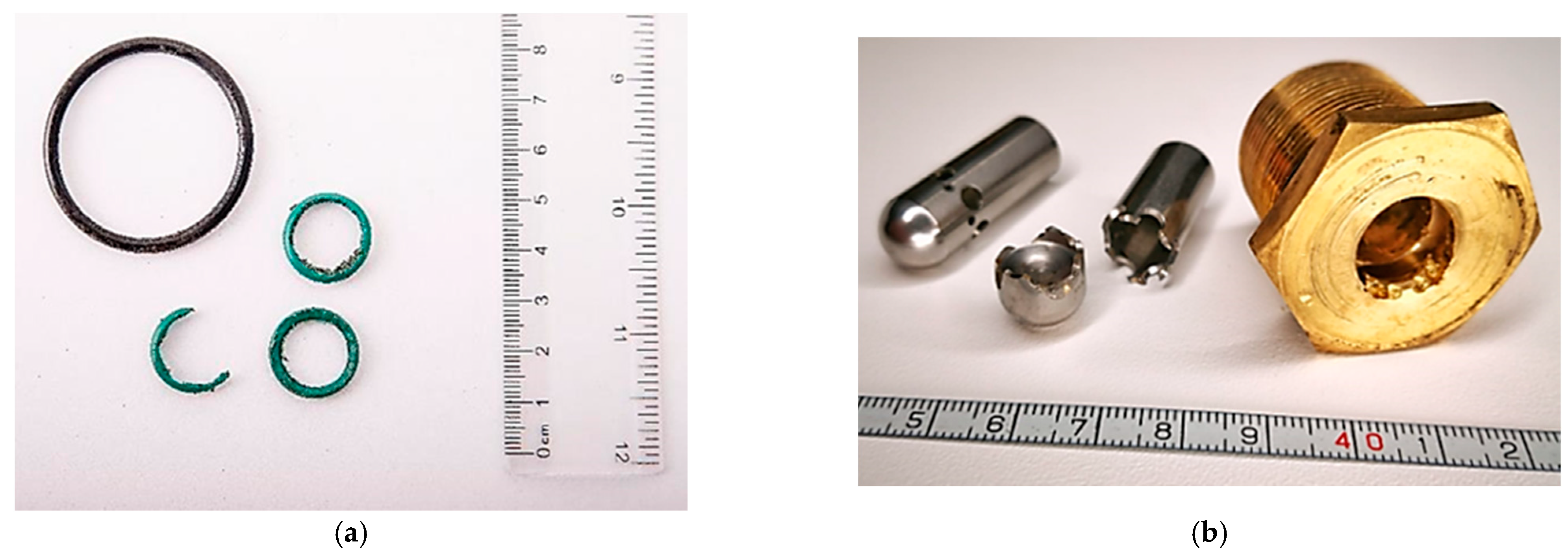
2. Safety Elements Damage

The safety elements of powered roof support are, in many cases, the last link securing the shields against damage due to rock tremors. The safety elements securing the hydraulic leg of a powered roof support against the damage are shown in Figure 1.

Putting the powered roof supports with large diameter hydraulic legs into the longwall operation requires increased flows of the liquid supplying the hydraulic legs, which entails technical problems resulting from the necessity to move a fluid with a high variability of pressure and intensity. These problems are especially exacerbated in the case of hydraulic legs in which the liquid from the working space (under the piston) is discharged to the operated check valve by drilling a hole in the hydraulic leg’s cylinder shell. Recently, cases of the operation of longwall supports were registered in which, despite compliance with all formal and technical requirements, there was an excessive amount of damage to the safety elements of powered roof supports. The recorded cases of damage events resulted from tremors of the rock mass, the values of which were lower than forecasted. The greatest amount of damage to the hydraulic leg’s control system components was recorded in shields in which hydraulic legs with a diameter of ∅ 0.37 m and drilled cylinder shells was used. The registered damage events during the advancing of the longwall showed that they were uniformly distributed along the entire longwall. Within four months of the longwall advance, over 500 cases of damage to various elements of the control hydraulics were recorded. The number and nature of these damage events during the longwall operation was enormous. A fragment of the data is shown in Figure 2. All recorded damage events occurred at the ends of the connections which discharge fluid from the working space of the hydraulic leg to the safety elements of the powered roof support, such as hydraulic legs, hydraulic valves and pressure gauges [17].

The damage always resulted in the loss of pressure in the hydraulic systems of the hydraulic legs, which in extreme cases resulted in the uncontrolled lowering of the shield height. This uncontrolled lowering meant that the longwall advances had to be stopped until the damage was dealt with. Hydraulic valves limiting the working pressure of the hydraulic legs (the overflow valves) were the elements that were most often damaged (representing approximately 50% of the damage incidents). The overflow valves used are piston valves with an O-ring seals and a spring (Figure 3). The damage was mainly in the form of damage to the O-ring seals sealing the valve piston, breaks or leaks of the piston and/or damage to the valve parts. Examples of damage are shown in Figure 4 [17].

In order to confirm the proper execution of the piston of the overflow valve (the basic element of the valve), the piston was subjected to chemical composition analysis in the laboratory of the Polish Mining Group (PGG S.A.). The chemical analysis showed that the chemical composition of the piston material was normal. Therefore, it should be assumed that the probable cause of the damage was the occurrence of pressures at the inlet of the hydraulic valve with values and variability exceeding its permissible technical parameters.

3. Materials and Methods

The model tests were performed using SolidWorks Flow Simulation, which is based on Computational Fluid Dynamics (CFD) as well as in SolidWorks Simulation (2018, Waltham, MA 02451, U.S.A) by the finite element method (FEM). This is a Computer-Aided Engineering (CAE), program used for designing 2D and 3D models, as well as allowing the creation of very detailed elements and assemblies at the design stage as well as working drawings. Also allow to inspect a design directly before production by means of a broad range of available tools, from CFD analysis to the analysis of static and dynamic strength of a studied prototype construction, based on the FEM method.

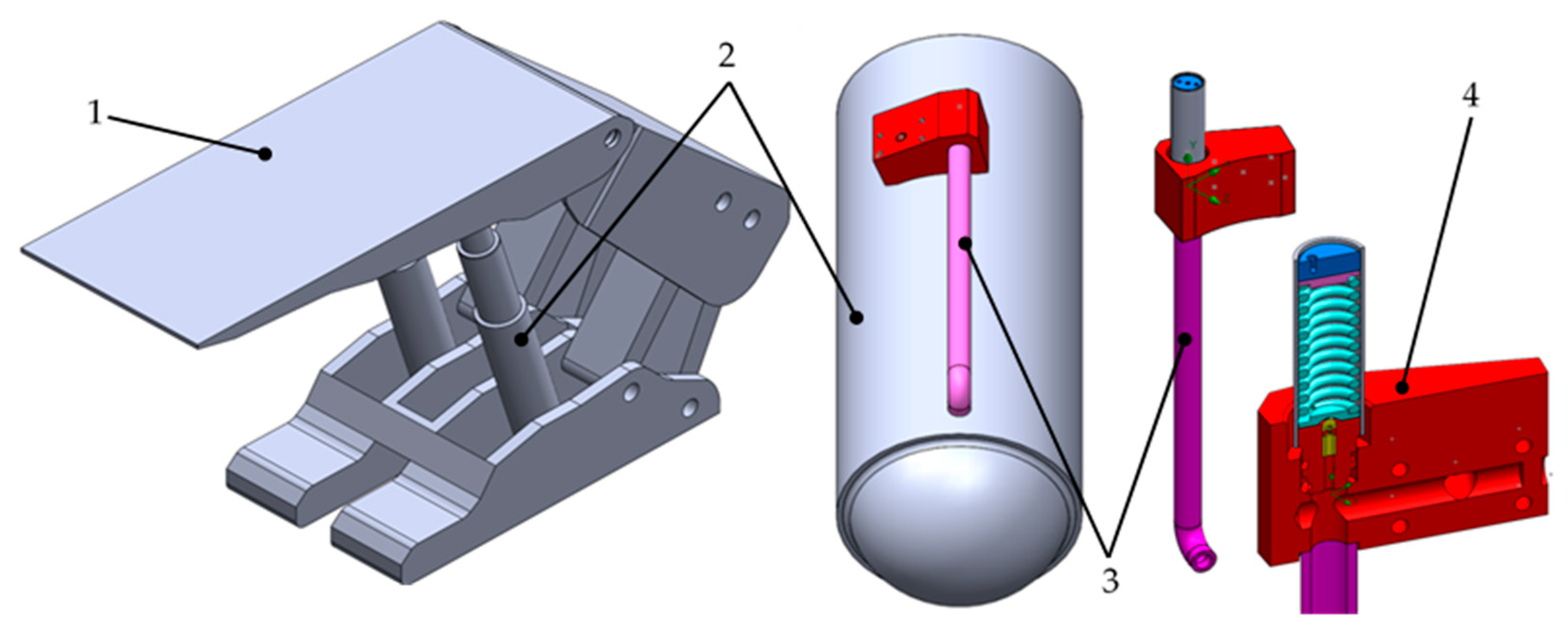
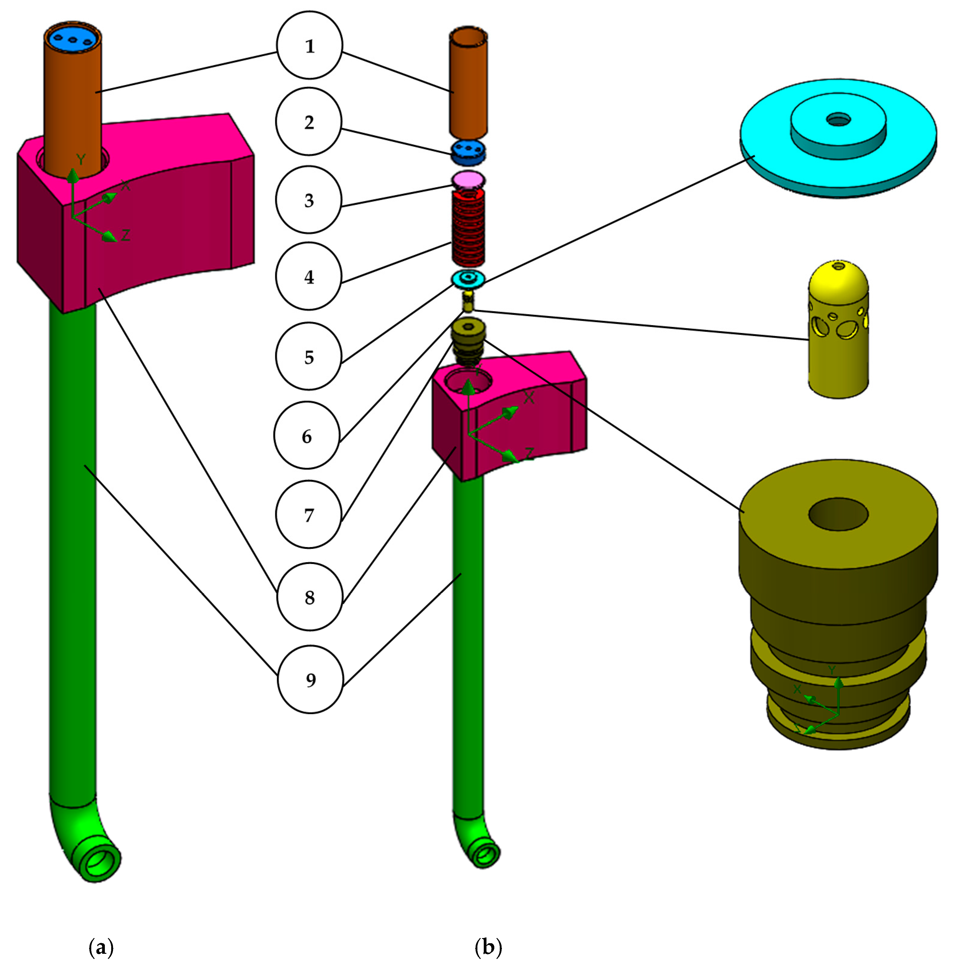
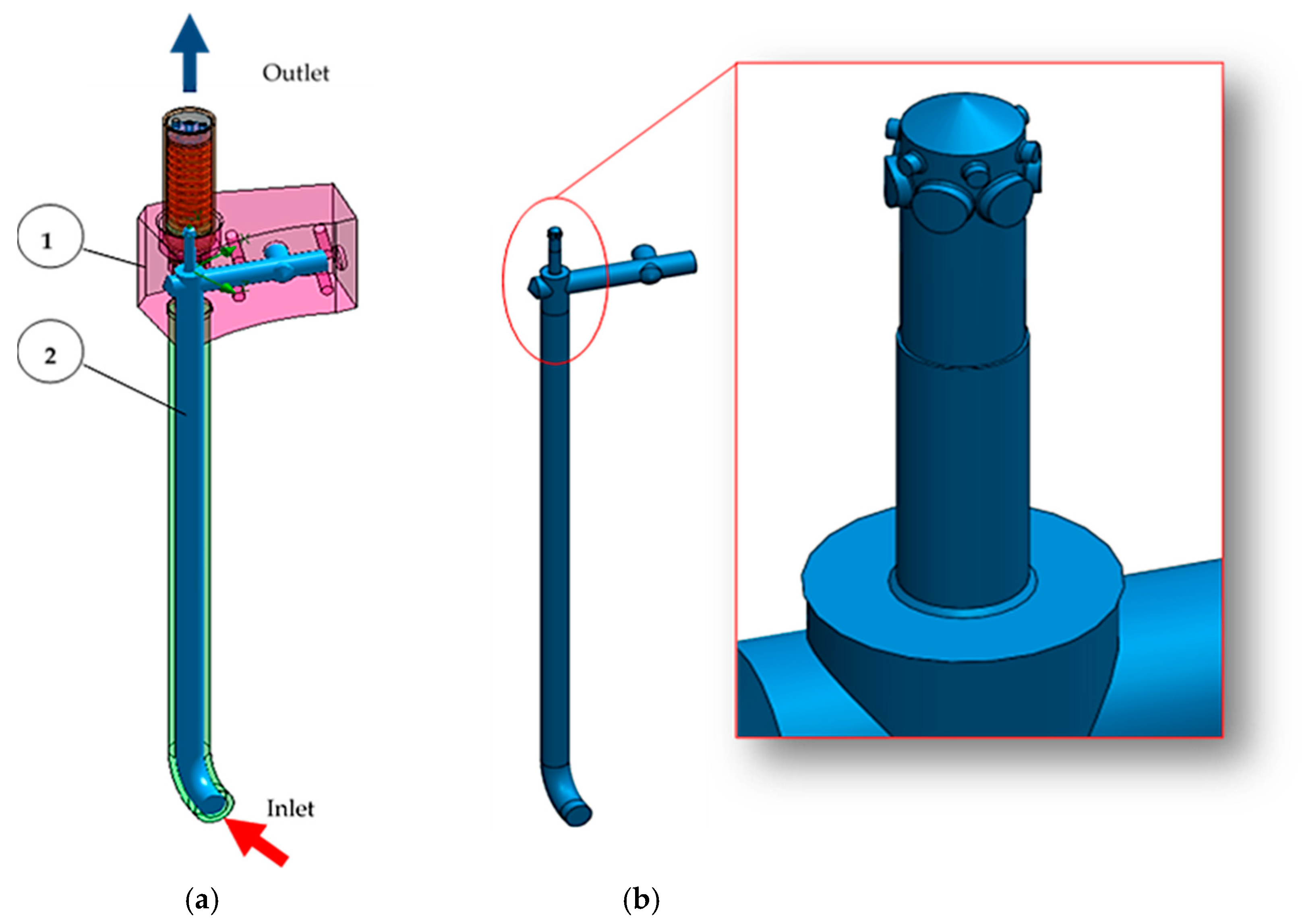
3.1. Geometry

In Figure 5 a view of the safety elements of a longwall shield is shown. The safety elements are the components of hydraulic legs which determine its power hydraulic as well as the safety and capacity of powered roof support. The main component of hydraulic legs is the overflow valve which serves as a safety valve. The overflow valve’s task is to protect and secure a hydraulic leg against dynamic loads which occur during rock burst. When the pressure in the hydraulic leg is exceeded then the overflow valve is opened via slide-piston (position 6 in Figure 5). The slide-piston with a roll spring (position 4 in Figure 5) acts directly on the adjusting nut (position 2 in Figure 5) and causes that the pressure is released in the hydraulic legs through the two holes located on the adjusting nut cover (position 1 in Figure 5).

Based on the 3D model, the volume of fluid was separated from solid geometry on which boundary conditions (i.e. volume flow rate, static pressure, etc.) are defined. The separated volume of fluid was used to generate the numerical model in order to simulate the work of safety elements using the CFD method. The CFD simulation will be able to predict the pressure change depending on the volume flow rate. The CFD results will be used to simulate load changes in the safety element using the finite elements method (FEM).

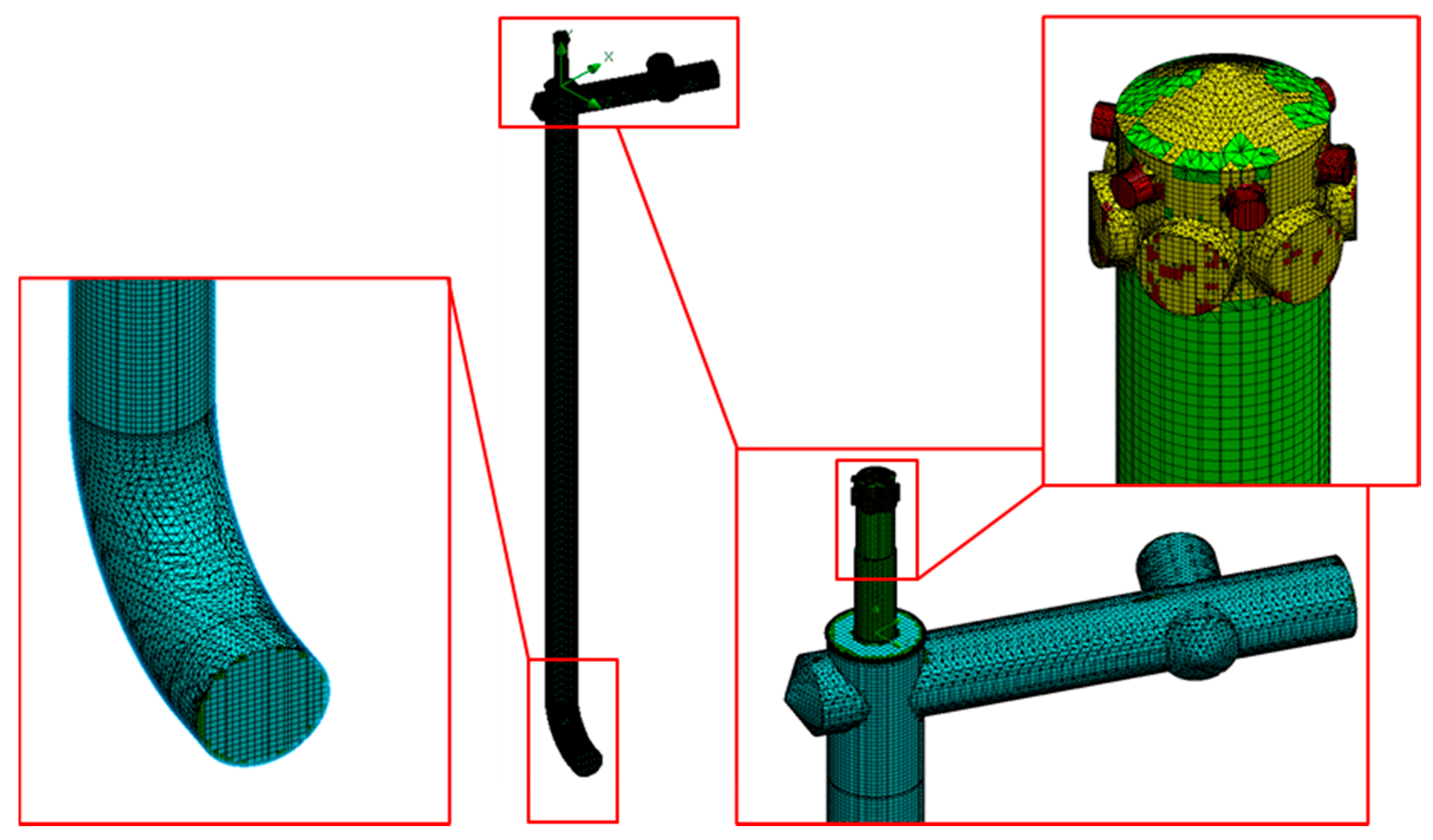
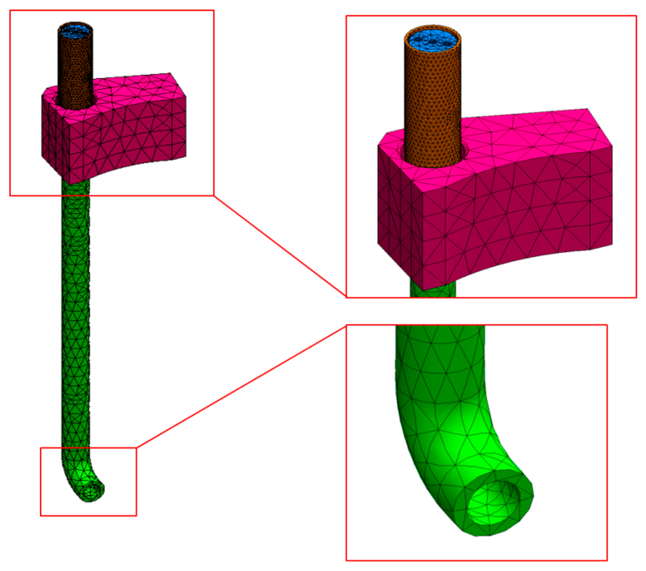
3.2. Numerical Grid

In the case of fluid flow analysis in the CFD module, the program groups fluid flow analysis into two separate categories namely: internal analysis and external analysis. At the beginning of model preparation, it is very important to recognize which type of analysis one wishes to perform; in this instance it is an internal flow analysis. For this type of analysis, the fluid enters a model through the inlets and exits the model through the outlets. In order to perform internal flow analysis, the overflow valve model must be fully closed (no openings) using lids. In Figure 6 the major steps of the fluid volume (Figure 6b) separating process based on the 3D model of safety elements (Figure 6a) are shown.

A numerical grid, shown in Figure 7, was formed by 226,112 total cells, where 69,745 fluid cells are in contact with solids, which represents the geometry of the fluid. The fluid volume is 0.0002 m³. The mesh grid was based on an orthogonal finite volume mesh.

In the case of safety element analysis, the modelling process begins by creating a geometric model. The program divides the model into small fragments with simple shapes (elements) that connect with each other at common points (nodes). Finite element analysis applications perceive the model as a grid of discrete elements which are connected to each other using the automatic generator. The automatic generator in the software generates a numerical grid based on the global information such as: tolerance, element size and determination of local mesh controls. Numerical grid control enables the specification of different element sizes for vertices, edges, faces and components. The program calculates the global element size for the model, taking into account its surface, area and volume. The size of the generated numerical grid (the number of nodes and elements) depends on the geometry and dimensions of the model, the size of the element, grid tolerance, grid control and specific contacts.

The numerical grid shown in Figure 8 was generated in the form of a mesh formed by 35,837 elements, connected with 62,804 nodes. The tetrahedral 3D solid elements for all solid components were used to generate the mesh grid.

3.3. Assumption of the CFD Method

The purpose of the fluid flow process simulation supported by CFD methods in the space that constitutes the volume occupied by the analyzed fluid is to obtain a solution to a set of differential equations which interpret the law of the conservation of the mass and momentum of the moving fluid (Naiver-Stokes equation). These fundamental equations, which express the behaviour of a fluid flow through a given geometry, are defined in the following forms [18]:

• Mass conservation equation:

  $$\frac{\partial \rho }{\partial t}+\nabla \left(\rho {\nu }_i\right)=0$$

  (1)
• Naiver-Stokes equation:

  $$\rho \frac{\partial \left(\rho {\nu }_i\right)}{\partial t}+\frac{\partial }{\partial x_j}\left(\varrho {\nu }_i{\nu }_j\right)+\frac{\partial P}{\partial x_i}=\frac{\partial }{\partial x_j}\left({\tau }_{ij+}{\tau }_{ij}^R\right)+S_i$$

  (2)

  where ρ–fluid density (kg·m⁻³), ν–fluid velocity (m·s⁻¹) and p–fluid pressure (Pa),

The influence of disturbances in the fluid transfer process within the given geometry were interpreted with a k-ε turbulence model. Solving this model comes down to determining the value of turbulent viscosity μ_t using turbulence kinetic energy k and dissipation rate ε related to the energy dissipation resulting from the occurrence of internal resistances to motion of a fluid flow through a channel. The turbulent viscosity μ_t model of the fluid is expressed using an equation defined in the following form:

$${\mu }_t=f_{\mu }{C}_{\mu }\frac{\rho k^2}{\epsilon }$$

(3)

Fluid transport equations for turbulence kinetic energy k and dissipation ε are expressed in the following forms [18]:

• For turbulence kinetic energy:

  $$\frac{\partial \rho k}{\partial t}+\frac{\partial \rho k{\nu }_i}{\partial x_i}=\frac{\partial }{\partial x_i}\left(\left(\mu +\frac{{\mu }_i}{{\sigma }_k}\right)\frac{\partial k}{\partial x_i}\right)+{\tau }_{ij}^R\frac{\partial {\nu }_i}{\partial x_j}-\rho \epsilon +{\mu }_t{P}_B$$

  (4)
• For dissipation energy:

  $$\frac{\partial \rho k}{\partial t}+\frac{\partial \rho \epsilon {\nu }_i}{\partial x_i}=\frac{\partial }{\partial x_i}\left(\left(\mu +\frac{{\mu }_i}{{\sigma }_k}\right)\frac{\partial \epsilon }{\partial x_i}\right)+C_{\epsilon 1}\frac{\epsilon }{k}\left(f_1{\tau }_{ij}^R\frac{\partial {\nu }_i}{\partial x_j}+C_B{\mu }_t{P}_B\right)-f_2{C}_{{\epsilon }_2}\frac{\rho {\epsilon }^2}{k}$$

  (5)

  where C_ε1–empirical constant, C_ε1 = 1.44, C_ε2–empirical constant, C_ε2 = 1.92, C_µ–empirical constant, C_µ = 0.09, k–velocity fluctuation (turbulence) kinetic energy (m²·s⁻²), P–local vorticity fluctuation production, ε– turbulence kinetic energy dissipation rate (m²·s⁻³), μ_t–turbulent viscosity (Pa·s), σ_k–turbulent Prandtl number σ_k = 1.0, σ_ε–turbulent Prandtl number σ_ε = 1.3 and µ–fluid dynamic viscosity (Pa·s).

In order to carry out the calculation process, the following boundary conditions were adopted for pure water:

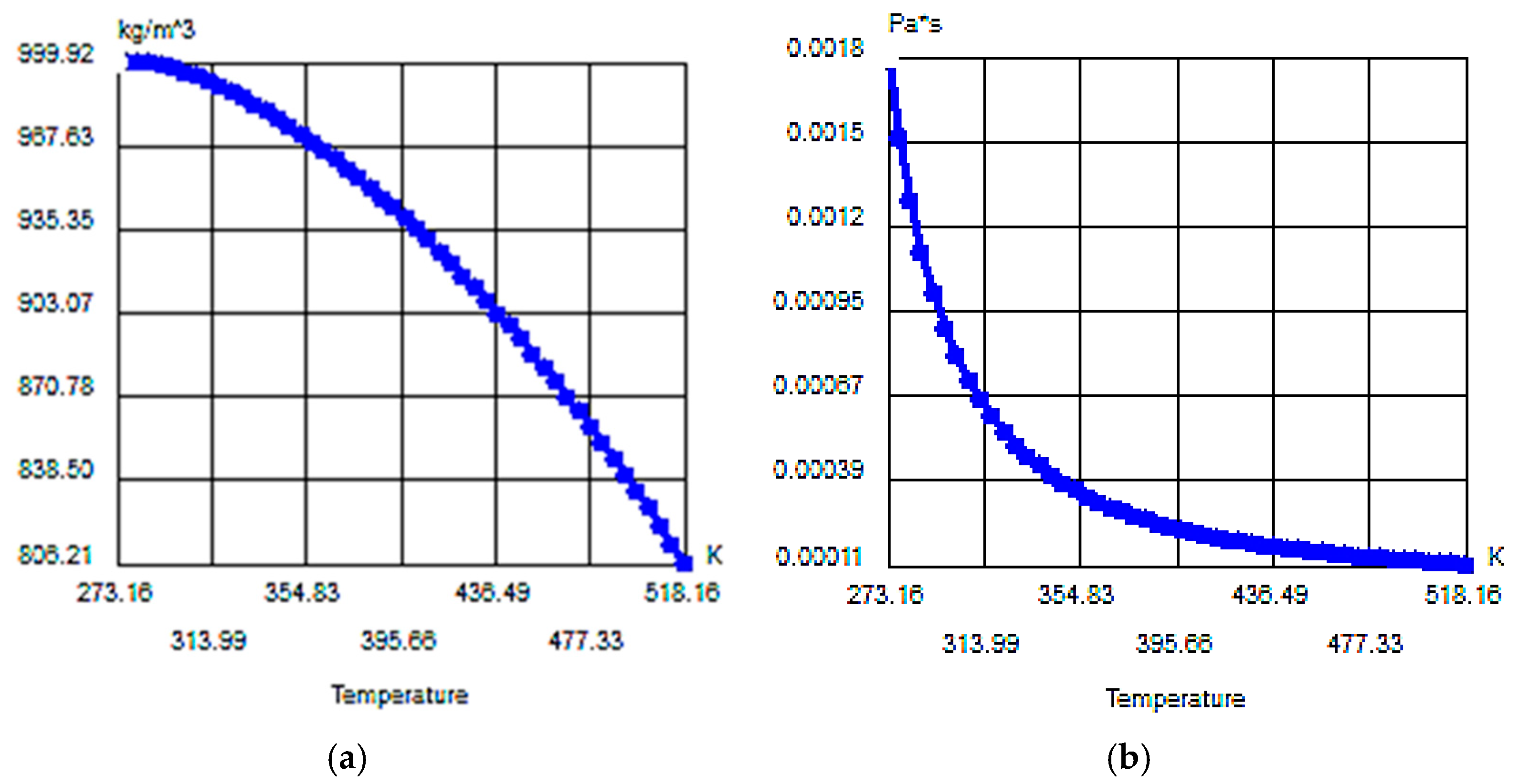
• density described by ρ(T) = −0.0025T² + 1.1577T + 871.45 (kg·m⁻³) (Figure 9a),
• dynamic viscosity described by µ(T) = 4 × 10⁻⁸ T² − 4 × 10⁻⁵ T + 0.0082 (Pa·s) (Figure 9b),
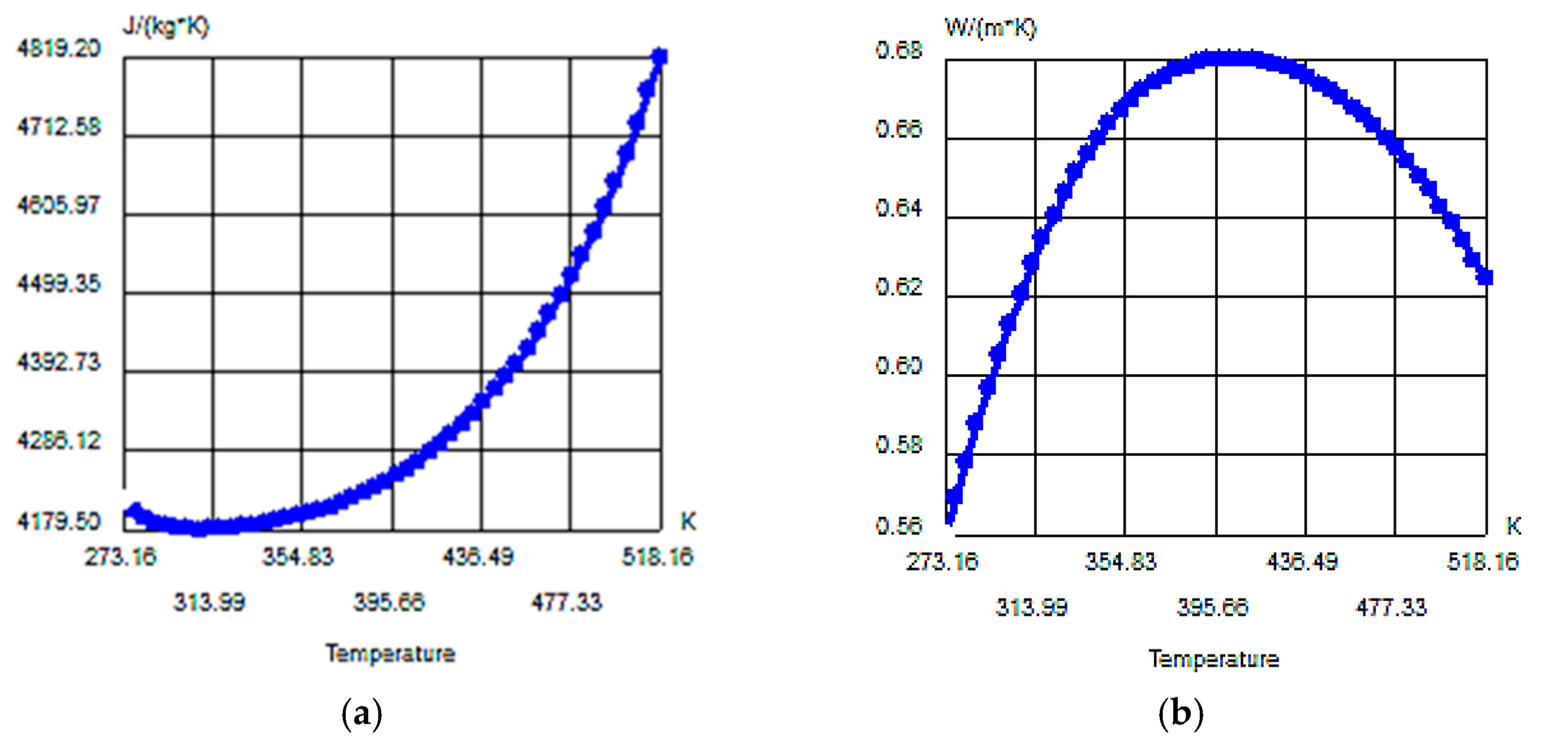
• specific heat described by C_p(T) = 0.0172T² − 11.4T + 6062.2 (J·kg⁻¹·K⁻¹) (Figure 10a),
• thermal conductive described by λ(T) = −6 × 10⁻⁶ T² + 0.005T − 0.332 (W·m⁻¹·K⁻¹) (Figure 10b),
• variation of volumetric flow V = 0 ÷ 2000 dm³·min⁻¹,
• temperature of fluid T = 298.15 (K) (25 °C).

3.4. Assumption of the Strength Analysis

Finite element analysis (FEM) is a numerical method for analyzing engineering projects. The software calculates the element size of the numerical grid for the overflow valve model, taking into account its volume, surface area and other geometric details. The size of the generated numerical grid (the number of elements and nodes) depends on the dimensions and geometry of the model, the size of the element, grid tolerance, grid control and specific contacts. At the initial stages of design analysis, when approximate results may be sufficient, a larger element size can be specified to reduce solution time. In order to obtain a more accurate calculation, a smaller size of the numerical grid may be required.

Calculations were carried out using the FEM method in SolidWorks Simulation. Computer programs, operating on the basis of the finite elements method numerical algorithms in addition to internal forces and displacements, automatically calculate the Huber-Mises-Hencky reduced tension in the following relationship [19]:

$${\sigma }_{red}=\sqrt{{\sigma }_x^2+{\sigma }_y^2+{\sigma }_z^2-{\sigma }_x{\sigma }_y-{\sigma }_x{\sigma }_z-{\sigma }_y{\sigma }_z+3\cdot \left({\tau }_{xy}^2+{\tau }_{xz}^2+{\tau }_{yz}^2\right)}$$

(6)

Equation (6) can be simplified to the following form [19]:

$${\sigma }_{red}=\sqrt{{\sigma }^2+3\cdot {\tau }^2}$$

(7)

where τ shear stresses (N·m⁻²), σ normal stresses (N·m⁻²).

By reducing the stresses into the appropriate loads related to the geometric properties W_x (the section modulus) for the cross-sectional area A, the following Equation (8) is obtained [19]:

$${\sigma }_{red}=\sqrt{{\left(\frac{Mg}{W_x}+\frac{N}{A}\right)}^2+3\cdot {\left(\frac{T}{A}\right)}^2}$$

(8)

where M_g–bending moment (Nm), N–axial force (N), T–shear force (transverse force) (N), W_x–section modulus (m³), A–cross section area (m²) and σ_red–normal stresses (N m⁻²),

4. Results

The results of numerical modelling were represented by curves in the graphs and in the form of graphically maps. The CFD method was used to calculate the pressure and the velocity for various values of volume flow rate in safety elements of the hydraulic leg. The volume flow rates in the CFD numerical model reflect and simulate the dynamic loads due to rock burst. The FEM method was used to calculate the effect of the pressure and the velocity on the distribution of stress contours reduced based on the Huber-Mises-Hencky hypothesis.

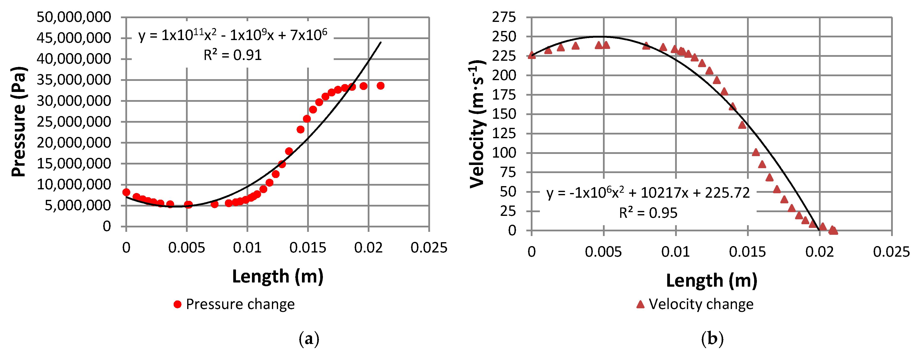
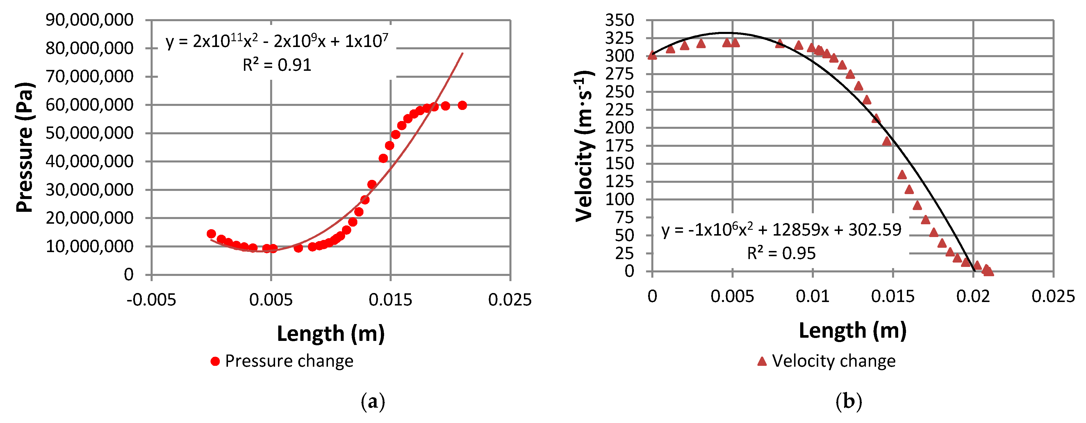
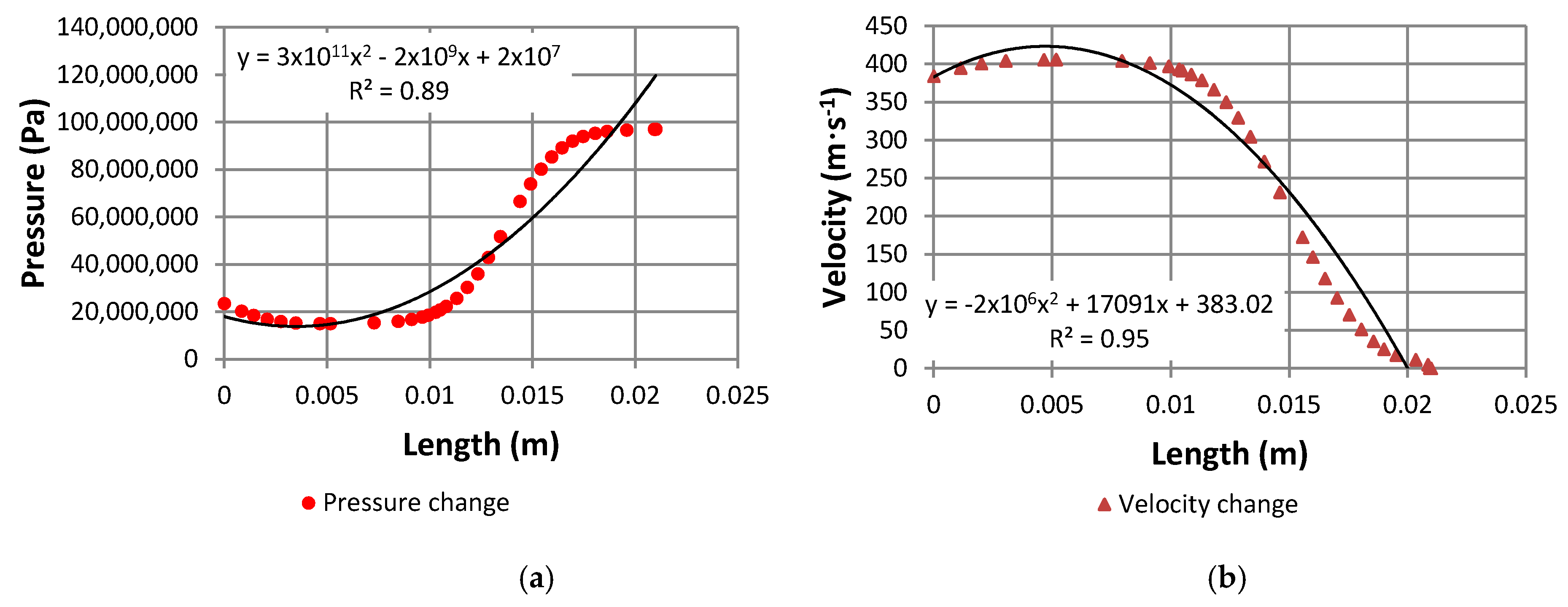
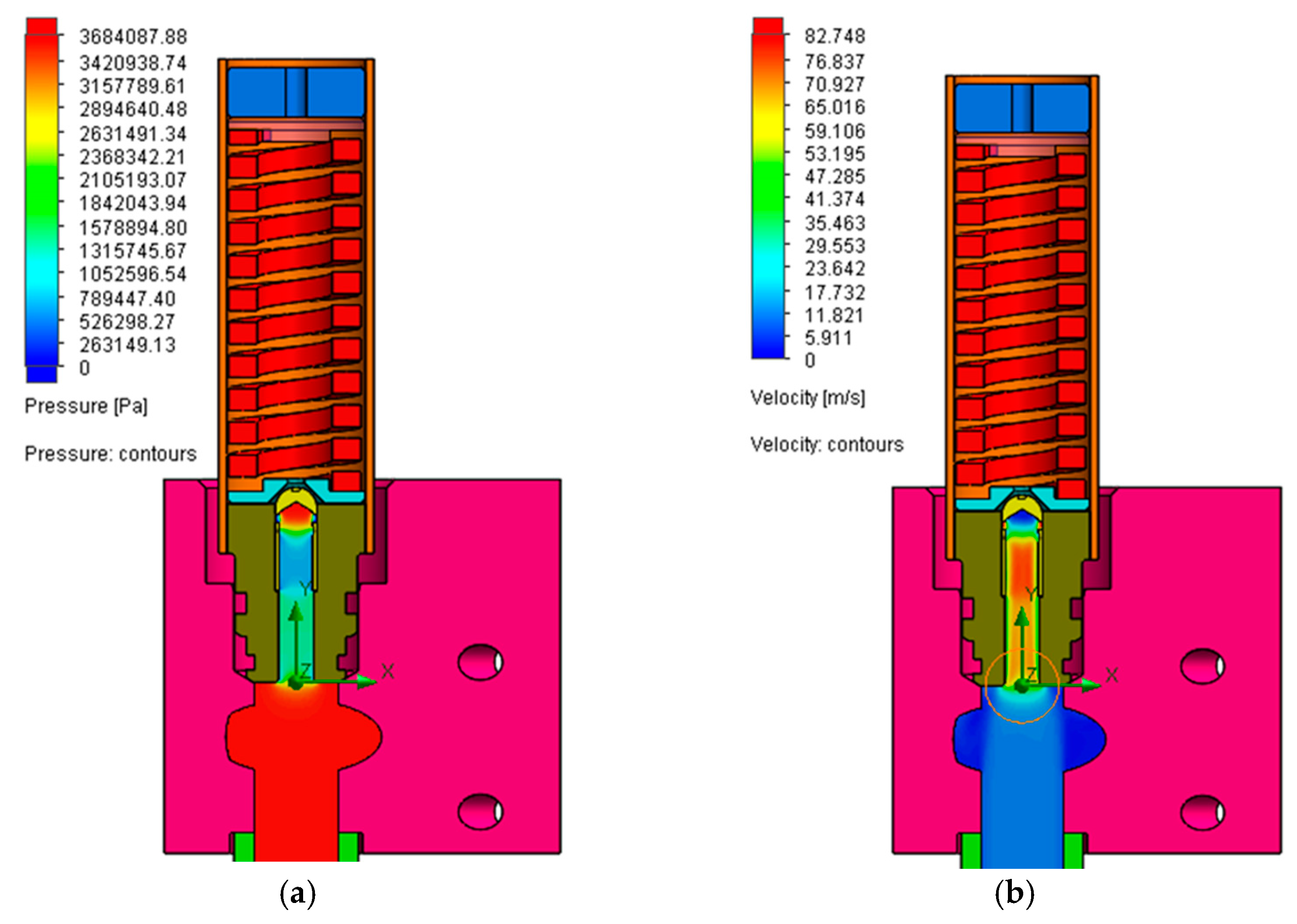
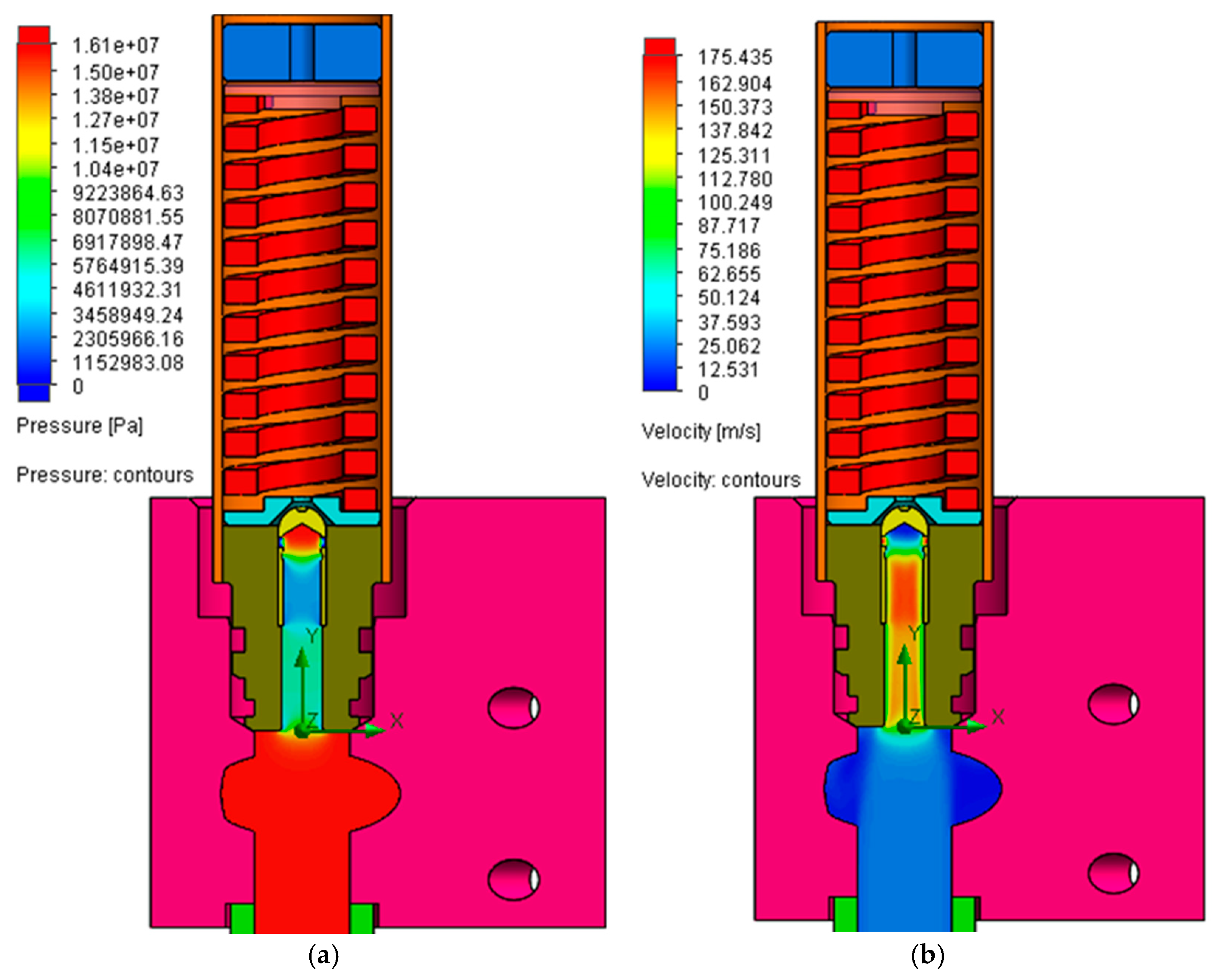
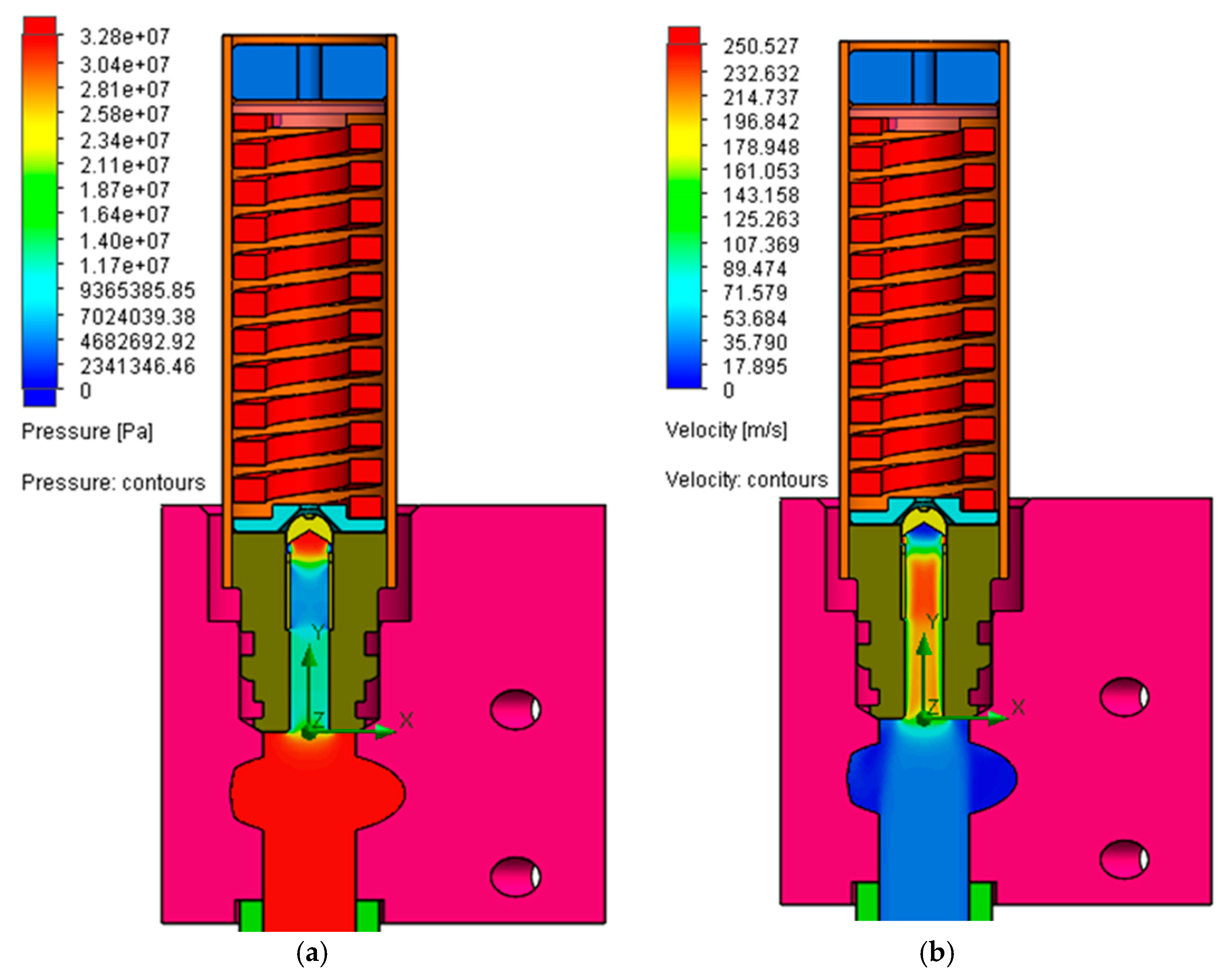
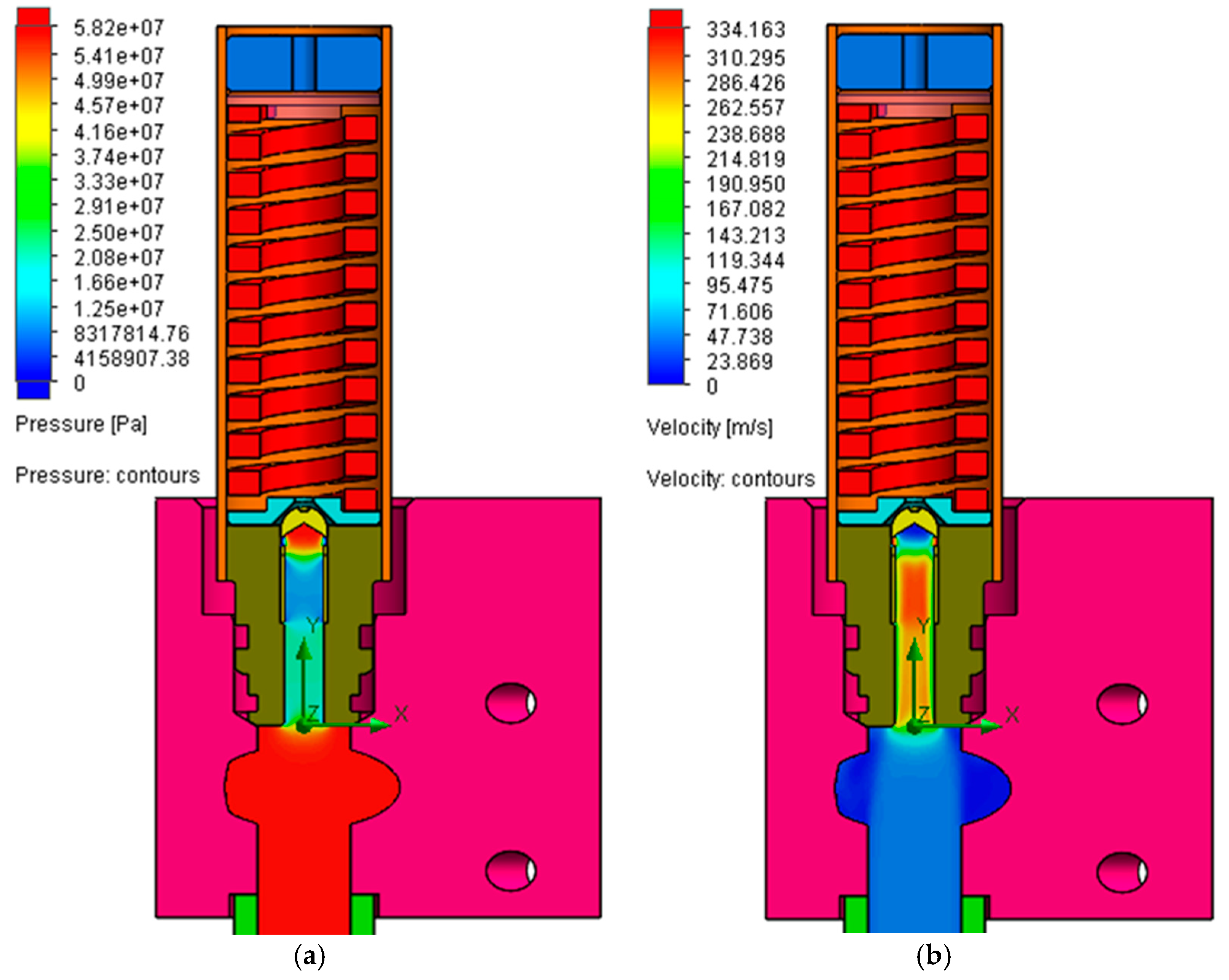
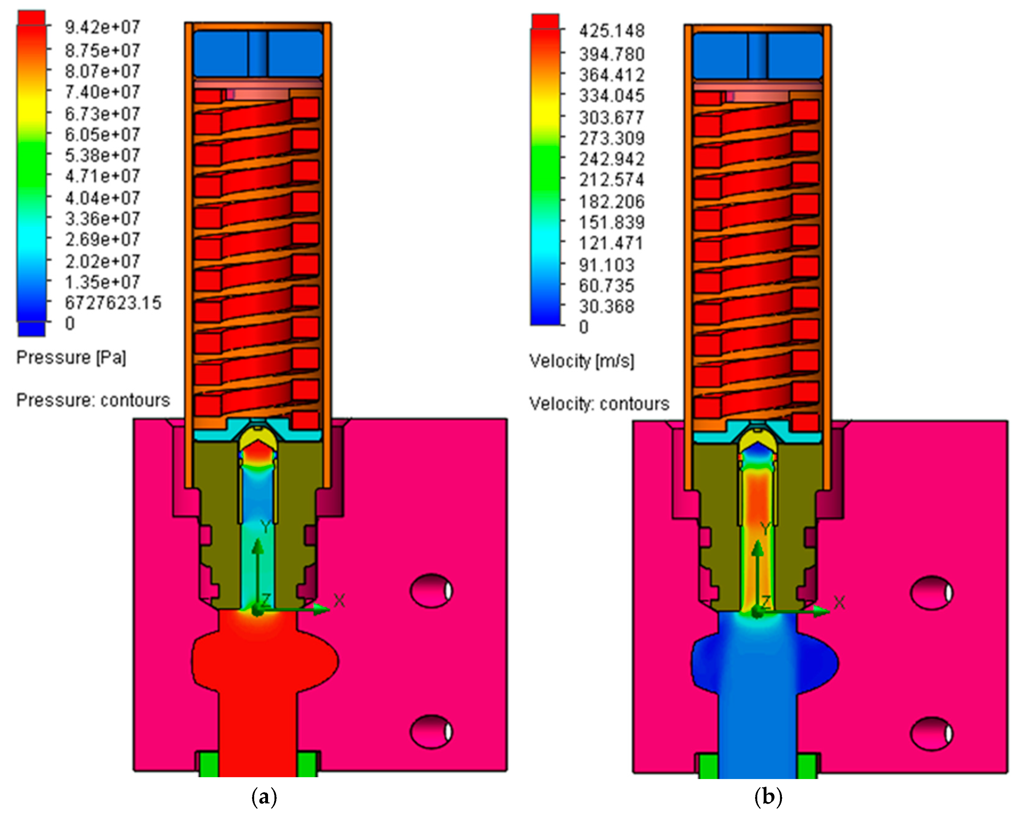
4.1. CFD Analysis

In Figure 11, Figure 12, Figure 13, Figure 14 and Figure 15 the results of our CFD simulations are presented. These figures illustrate the characteristics of slide-piston (position 6 in Figure 5) work for different values of volume flow rate. The horizontal axis describes the change of slide-piston length. The length of the slide-piston is 0.022 m. The vertical axis describes the change of pressure and velocity along the length of the slide-piston. The results were obtained from numerical calculations using the CFD. The volume flow rate simulates loading by a rock burst.

The pressure-length curve in Figure 11a shows that pressure changes in a range from approx. 1 × 10⁶ Pa, at the slide-piston inlet, to approx. 4 × 10⁶ Pa, at the slide-piston outlet, for a volume fluid flow which equals 0.0033 m³s⁻¹. In the case of the results in Figure 11b, the velocity-length curve shows that the velocity is 70 m·s⁻¹ at the slide-piston outlet but the velocity at the outlet is 0.02 m·s⁻¹.

The pressure-length curve in Figure 12a shows that pressure change in the range from approx. 5 × 10⁶ Pa, at the slide-piston inlet, to approx. 15 × 10⁶ Pa, at the slide-piston outlet, for a volume fluid flow which equals 0.007 m³·s⁻¹. In the case of the results in Figure 12b, the velocity-length curve shows that the maximum value of velocity is 180 m·s⁻¹ but at the outlet the velocity is 0.02 m·s⁻¹.

The pressure-length curve in Figure 13a shows that pressure change in the range from approx. 10 × 10⁶ Pa, at the slide-piston inlet, to approx. 35 × 10⁶ Pa, at the slide-piston outlet, for a value of volume fluid flow which equals 0.01 m³·s⁻¹. In the case of the results in Figure 13b, the velocity-length curve shows that the maximum value of velocity is 250 m·s⁻¹ at the slide-piston inlet but at the outlet the velocity is 0.02 m·s⁻¹.

The pressure-length curve in Figure 14a shows that pressure change in the range from approx. 10 × 10⁶ Pa, at the slide-piston inlet, to approx. 60 × 10⁶ Pa, at the slide-piston outlet, for a value of volume fluid flow which equals 0.01335 m³·s⁻¹. In the case of the results in Figure 14b, the velocity-length curve shows that the maximum value of velocity is 350 m·s⁻¹ at the slide-piston inlet but at the outlet the velocity is 0.02 m·s⁻¹.

The pressure-length curve in Figure 15a shows that pressure changes between approx. 20 × 10⁶ Pa, at the slide-piston inlet, to approx. 100 × 10⁶ Pa, at the slide-piston outlet, for a value of volume fluid flow which equals 0.017 m³·s⁻¹. In the case of the results in Figure 15b, the velocity-length curve shows that the maximum value of velocity is 425 m·s⁻¹ but at the outlet the velocity is 0.02 m·s⁻¹.

The results of CFD simulations show an increase of pressure by 19 × 10⁶ Pa at the inlet slide-piston, where for velocity the results show an increase by 365 m·s⁻¹. In the case of pressure, the results show an increase of 96 × 10⁶ Pa at the outlet of the slide-piston.

Figure 16, Figure 17, Figure 18, Figure 19 and Figure 20 show the variation of pressure and velocity in the safety elements of a longwall shield in the form of graphic maps. The results were listed depending on the volume flow rate of the fluid. The qualitative analysis supporting the interpretation of the results shows that the pressure reaches its maximum value at the inlet of the connecting spigot (position 7 in Figure 7) and at the outlet of the slide-piston (position 6 in Figure 5). In the case of velocity, the maximum value was reached along the length of the slide-piston and the connecting spigot.

In the area where CFD calculation achieves the maximum value of pressure and velocity, the damage to the safety elements can occur. The strength analysis will be performed using the FEM method to clarify the obtained results of the CFD calculations.

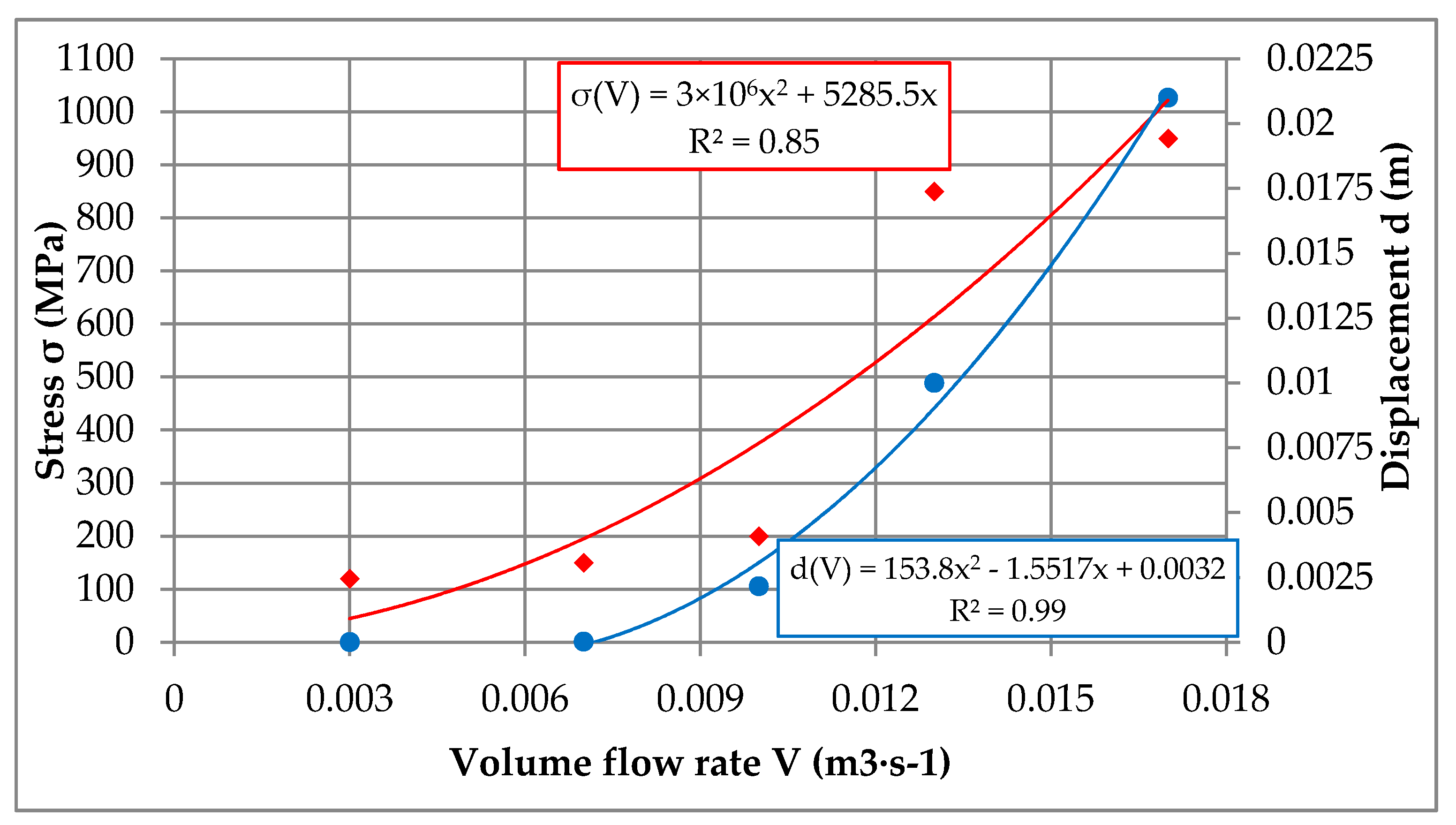
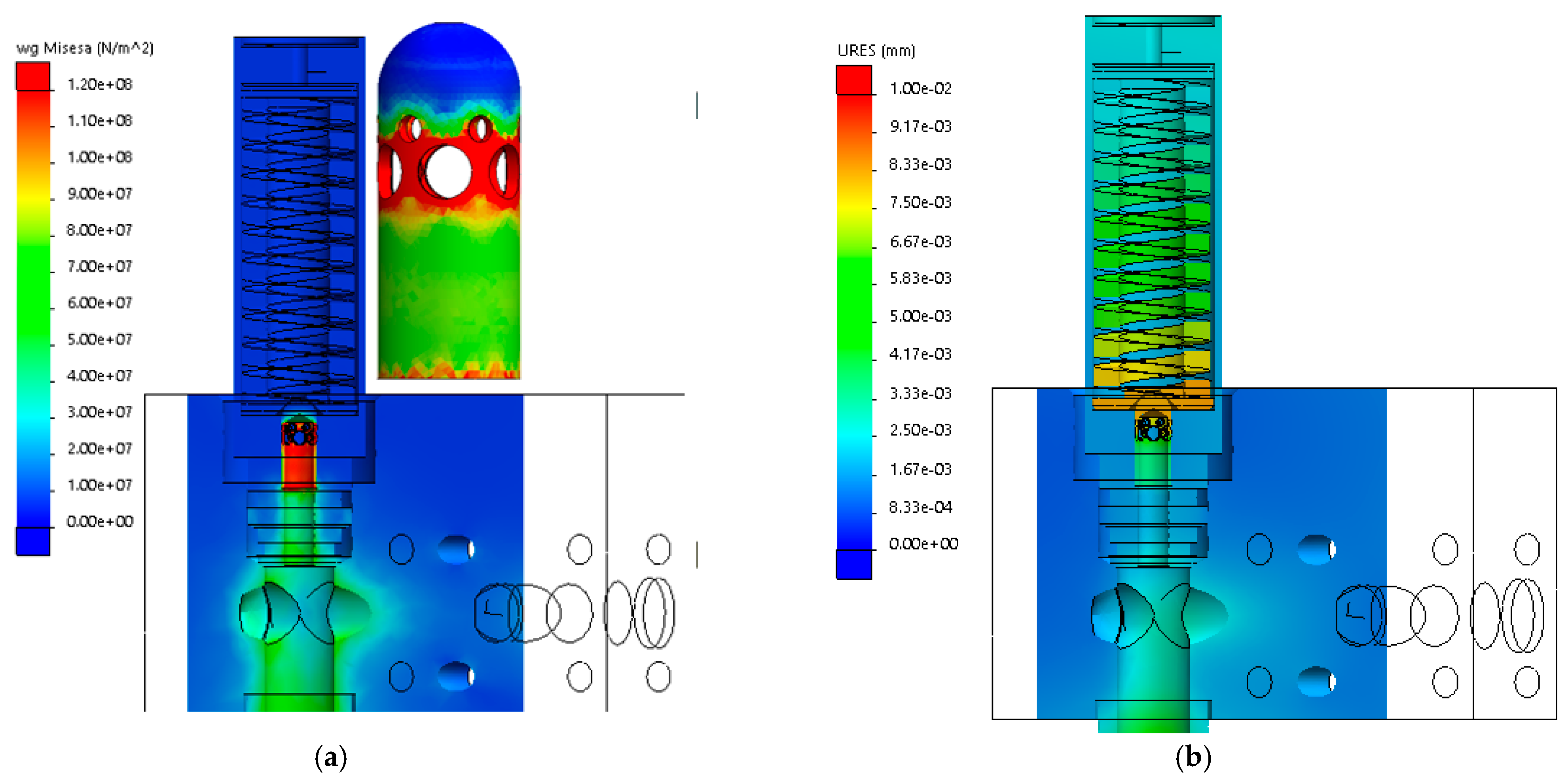
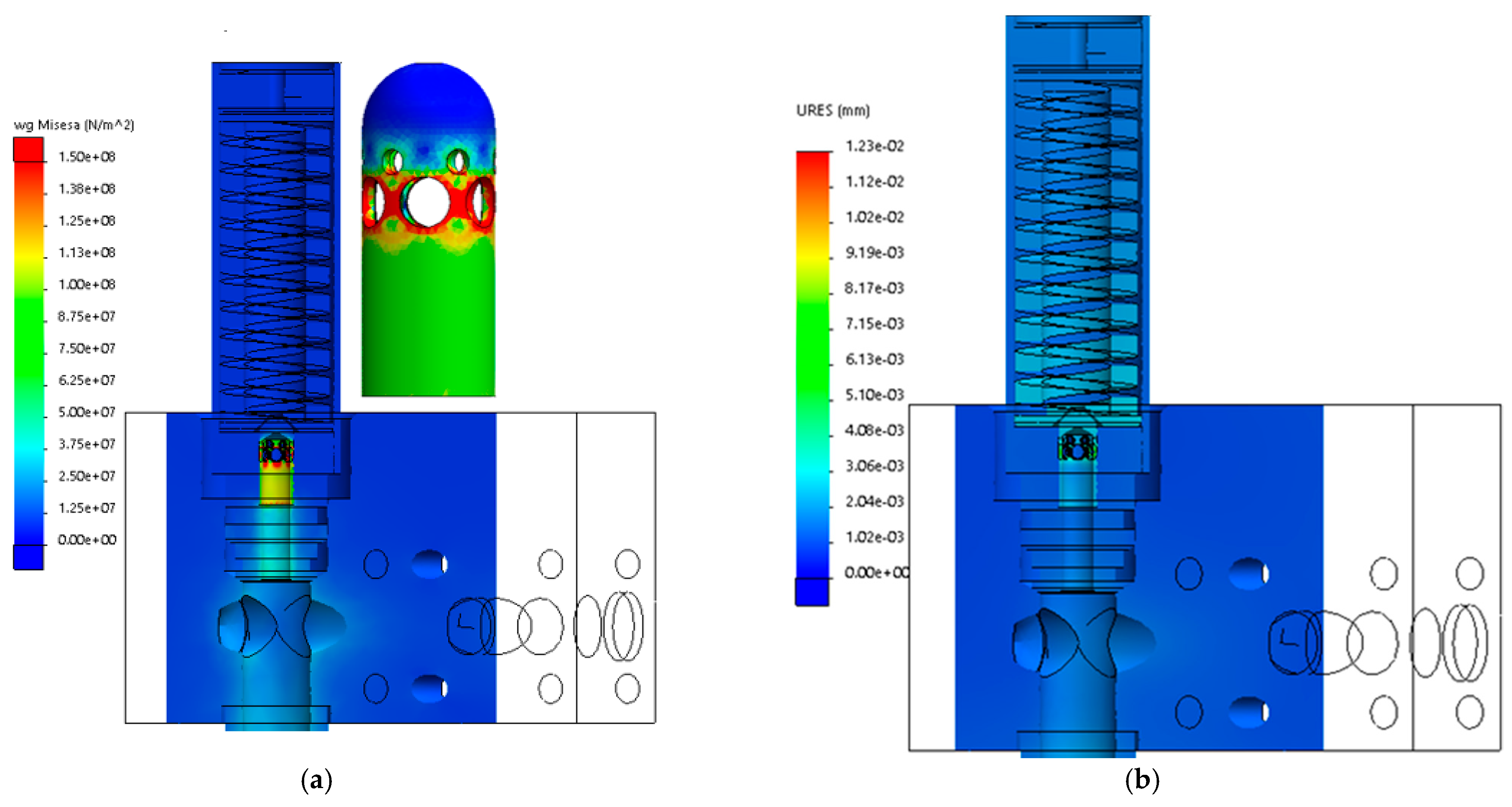
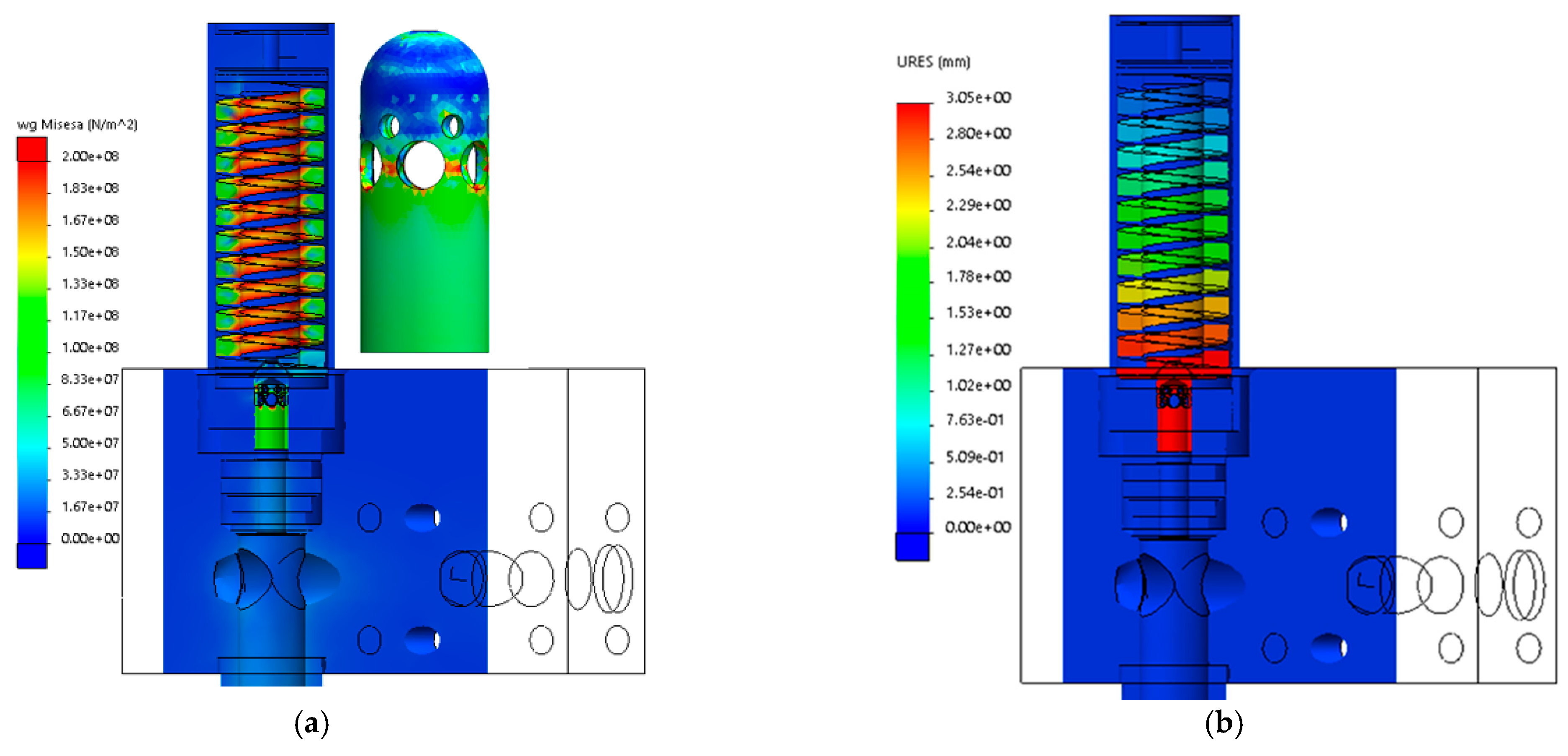
4.2. Strength Analysis

The curve in Figure 21 illustrates the variation of the von Mises stress and the displacement depending on the volume flow rate. The horizontal axis describes the change of the volume flow rate. The vertical axis describes the change of stress and displacement. Results were obtained from numerical calculations using the FEM method. The von Mises criteria was used in order to determine stress value in the safety elements which was subjected in a complex loading condition. The results of the von Mises stress were compared with the material’s tensile strength (R_m).

The stress-volume flow rate curve in Figure 21 shows that the increase of stress in the analyzed safety elements of longwall hydraulic power support occurs above the volume flow rate value of 0.0025 m³·s⁻¹. It can be noticed that the higher the value of the volume flow rate, the greater is the stress in the safety elements.

Table 1. Change of von Misses stress (δ) and displacement (d) depending on the volume flow rate of the fluid.

No.	Stress σ, (MPa)	Displacement d, (m)	Volume Flow Rate V, (m3·s−1)
1.	120	0.000012	0.003
2.	150	0.000031	0.007
3.	200	0.002160	0.010
4.	850	0.010000	0.013
5.	950	0.021000	0.017

illustrates the variation of stresses and displacement due to pressure in safety elements.

Figure 22, Figure 23, Figure 24, Figure 25 and Figure 26 show the variation maps of von Mises stress and displacement in the safety elements of the longwall shield. The results are shown in the form of graphic maps depending on the volume flow rate of the fluid. The qualitative analysis of the results in Figure 22, Figure 23, Figure 24, Figure 25 and Figure 26 show that von Mises stress reaches its maximum value in the slide-piston (position 6 in Figure 5). Up to the amount of 0.01 m³·s⁻¹, the von Mises stress is not exceeded in the safety elements. Above the value of 0.01 m³·s⁻¹, the von Mises stress is exceeded and this occurs mainly in the slide-piston. The yield point (R_e) of the slide-piston steel is 650 MPa, but the variation of tensile strength (R_m) between 800–1000 MPa [20].

It can be observed in Figure 22, Figure 23, Figure 24, Figure 25 and Figure 26 that destruction of the overflow valve is the result of notches appear on the surface, which led to cracks and consequently damage to the slide-piston due to exceeding permissible stresses above 0.01 m³·s⁻¹.

5. Discussion

The safety elements are the key system of the hydraulic leg which securing a powered roof support against damage and the uncontrolled lowering of shield height during the mining process. The uncontrolled lowering of shields height can cause the danger of the loss of the longwall stability in the form of a rock bursts and collapses as well as danger to safety and health for employees.

Using the CFD method described in the paper, the pressure and velocity developments in the safety elements of the 2-leg shield were simulated and calculated. Based on the results of CFD calculations the effect of the pressure and the velocity on the distribution of stress contours reduced based on the Huber-Mises-Hencky hypothesis were simulated and calculated. The applying the CFD method with connection of strength analysis by FEM method have enabled captured the main process and mechanisms of damage. These phenomena cannot be monitored experimentally or in the laboratory conditions due to huge investment costs caused by the highly dynamic process, measured in microseconds.

The novelty demonstrated in the paper is to develop a numerical method for selecting overflow valve for dynamic load conditions by means of the CFD method and strength analysis using the FEM method in the hydraulic system of longwall powered support.

Connecting these two methods allows to observe the interaction of various factors, the effect of which is greater than the sum of individual separate actions (the synergies of calculations). The proposed method of numerical calculation for investigation of hydraulic system by the case of the 2-leg shield was not reflected in available literature. There is a wide range of method for an analysis of hydraulic leg safety system reported by various researchers [14,15,16] but does not include the possibility of addressing this problem.

Presented in the paper numerical model is a hybrid approach combining the CFD method with the strength analysis by FEM method allows a better understanding of the hydraulic leg safety elements behaviour under the dynamic load in the context of effectiveness of hydraulic system as well as can be a one of the method for selecting shields to geo-mining conditions. Moreover, the numerical model can be adapted to the actual situation based on an available experimental monitoring.

6. Conclusions

This article presents the results of model tests which consisted of identifying the distribution of the pressure and the stresses causing the destruction of the overflow valve piston. Model tests were carried out with the use of the CFD method to determine the fluid pressure in the safety system of 2-leg shield and the strength analysis by FEM method in order to determine the distribution of stresses based on the Huber-Mises-Hencky hypothesis.

The results of the model tests allowed to identify the safe scope of the overflow valve work for the considered case of the powered roof support to the value of volume flow rate below 0.01 m³·s⁻¹, which corresponds to a reference value of 600 L·min⁻¹ and pressure approx. 35 × 10⁶ Pa. The results of the model tests enabled the formulation of the following conclusions:

(1)

The use of CFD methods in combination with the finite element methods (FEM) enables the identification of the pressure values and the von Mises stress in safety elements of the powered roof support which may leads to its destruction as a result of dynamic loads originating from the rock mass occurs during the longwall mining,

(2)

The results of numerical simulations have made it possible to identify the maximal scope of the overflow valve work below the volume flow rate approximately 0.01 m³·s⁻¹, which corresponds to a reference value of 600 L·min⁻¹,

(3)

Results of the strength analysis by finite element method allowed identifying the reasons of damage in safety system of hydraulic legs by specifying a higher stress value than allowable for the piston material,

(4)

The exceeded values of stress observed in the piston based on the numerical strength analysis by FEM method led to damage to safety system of the hydraulic leg which covers with the real observations,

(5)

The results of model tests have created the possibilities to enhance the use of the analyzed overflow valve, through modifications of the geometry of the overflow valve piston and increase the strength parameters of the material,

(6)

The combination of CFD methods with the strength analysis by FEM methods provided for development a method enabling the effective design and method for selection of the powered roof support to given dynamic load conditions,

(7)

The advantages of proposed method are the possibility of adaptation the numerical model to the actual situation based on an available experimental monitoring,

(8)

The numerical calculations demonstrated that the coupled CFD method together with the strength analysis based on the FEM method adopted in this paper can give good insights into the hydraulic system dynamic behaviour of the powered roof support.

References

- Kabiesz, J.; Konopko, W.; Patyńska, R. Annual Report on the State of Basic Natural and Technical Hazards in Hard Coal Mining; GIG: Katowice, Poland, 2020; pp. 97–101. [Google Scholar]
- Ordinance of the Minister of Energy on Detailed Requirements for Conducting Underground Mining Operations of 23 November 2016. Available online: http://www.dziennikustaw.gov.pl/du/2017/1118/1 (accessed on 5 November 2019).
- Prusek, S.; Rajwa, S.; Stoiński, K. Kriterien zur Abschätzung des Risikos von Strebschaden; Glückauf-Forschung,66, 3;92–95. 2005. Available online: https://www.tib.eu/de/suchen/id/tema:TEMA20051107016/Kriterien-zur-Absch%C3%A4tzung-des-Risikos-von-Strebsch%C3%A4den?cHash=db8855764c5376dd561b7de3fce57f98 (accessed on 5 November 2019).
- Rajwa, S.; Prusek, S.; Stoiński, K. The principles of Powered roof Support Yielding—Method Description; Work Safety and Environmental Protection in Mining, No. 12; 2016; pp. 3–8.
- Stoiński, K. Mining Roof Support in Hazardous Conditions of Mining Tremors; The Central Mining Institute: Katowice, Poland, 2000. [Google Scholar]
- Stoiński, K. Powered Roof Support for Rock Tremors Conditions; The Central Mining Institute: Katowice, Poland, 2018. [Google Scholar]
- Świątek, J.; Stoiński, K. Case Analysis of Damages to Control Hydraulics of the Leg in the Powered Roof Support Section; E3S Web of Conferences, 105, 03013(2019). Available online: https://www.e3s-conferences.org/articles/e3sconf (accessed on 5 November 2019). [CrossRef]
- Peng Syd, S.; Cheng, J.; Du, F.; Xue, Y. Underground ground control monitoring and interpretation, and numerical modeling, and shield capacity design. Int. J. Min. Sci. Technol. 2019, 29, 79–85. [Google Scholar] [CrossRef]
- Brown, F.T. The Transient Response of Fluid Lines. J. Basic Eng. Trans. ASME Ser. D. 1962, 84, 547–553. [Google Scholar] [CrossRef]
- Rajwa, S.; Janoszek, T.; Świątek, J. The Simulation of Fluid Flow in Safety Elements of Longwall Shield Support Hydraulic Legs; IOP Conf. Ser.: Mater. Sci. Eng. 679 012017. Available online: https://0-iopscience-iop-org.brum.beds.ac.uk/article/10.1088/1757-899X/679/1/012017 (accessed on 5 November 2019). [CrossRef]
- Rajwa, S.; Janoszek, T.; Prusek, S. Influence of canopy ratio of powered roof support on longwall working stability—A case study. Int. J. Min. Sci. Technol. 2019, 29, 591–598. [Google Scholar] [CrossRef]
- Stoiński, K. Selection of Hydraulic Prop Longwall Support for Work in Conditions of Rock Mass Tremors Hazard; Archives of Mining Sciences: Kraków, Poland, 1998; Volume 43, pp. 471–486. [Google Scholar]
- Świątek, J.; Szurgacz, D. The Identification of the Damage Causes of the Hydraulic Control System Components in Powered Roof Support by Means of Tests and Calculations; AIP Conference Proceedings 2209, 020003 (2020). Available online: https://aip.scitation.org/doi/10.1063/5.0000011 (accessed on 5 November 2019). [CrossRef]
- Szurgacz, D.; Brodny, J. Adapting the Powered Roof Support to Diverse Mining and Geological Conditions. Energies 2020, 13, 405. [Google Scholar] [CrossRef] [Green Version]
- Janota, M.; Władzielczyk, K. The Use of the CFD Method to Calculate the Fluid Dynamics in By-Pass Valves of Power Supports; Mining–Informatics, Automation and Electrical Engineering, Vol. 52, No. 5; 2014; p.49–55. Available online: http://yadda.icm.edu.pl/yadda/element/bwmeta1.element.baztech-b1f54c36-a337-451f-a815-66b97e1056d5 (accessed on 5 November 2019).
- Cymerys, A.; Władzielczyk, K. Work Analysis of Working Overflow Valve by Means of the CFD Method in the Hydraulic System of Longwall Powered Support Set; Przegląd Górniczy, Vol. 67, No. 11; 2011; pp. 98–105. Available online: http://yadda.icm.edu.pl/yadda/element/bwmeta1.element.baztech-b7cca520-2f3b-443e-be48-8b2a39f434e4?q=bwmeta1.element.baztech-419e187b-4773-48e1-85ab-1171cb143e6a;13&qt=CHILDREN-STATELESS (accessed on 5 November 2019).
- Świątek, J. The Method to Improve the Operation of the Hydraulic Leg of a Powered Roof Support. Ph.D. Thesis, Central Mining Institute, Katowice, Poland, 2020. (Unpublished). [Google Scholar]
- Sobachkin, A.; Dumnov, G. Numerical Basis of CAD-Embedded CFD; NAFEMS World Congress; Salzburg, Austria. 2013. Available online: https://www.semanticscholar.org/paper/Numerical-Basis-of-CAD-Embedded-CFD-White-Sobachkin-Dumnov/56f54b31c528c588cfb465d953c2b0f24ea9e297 (accessed on 5 November 2019).
- Grodzicki, M.; Rotkegel, M. The Concept of Modification and Analysis of the Strength of Steel Roadway Supports for Coal Mines in the Soma Basin in Turkey; Studia Geotechnica et Mechanica; 2018; 40(1): 38–45. Available online: https://content.sciendo.com/configurable/contentpage/journals$002fsgem$002f40$002f1$002farticle-p38.xml (accessed on 5 November 2019).
- Polish Standard—PN-EN 10088-1:2014-12. Stainless Steels. Part 1: List of Stainless Steels; Polish Committee for Standardization (PKN): Warsaw, Poland, 2014. [Google Scholar]