Impact of Actual Weather Datasets for Calibrating White-Box Building Energy Models Base on Monitored Data

Gutiérrez González, Vicente; Ramos Ruiz, Germán; Fernández Bandera, Carlos

doi:10.3390/en14041187

Open AccessArticle

Impact of Actual Weather Datasets for Calibrating White-Box Building Energy Models Base on Monitored Data

by

Vicente Gutiérrez González

,

Germán Ramos Ruiz

and

Carlos Fernández Bandera

^*

School of Architecture, University of Navarra, 31009 Pamplona, Spain

^*

Author to whom correspondence should be addressed.

Energies 2021, 14(4), 1187; https://0-doi-org.brum.beds.ac.uk/10.3390/en14041187

Submission received: 23 December 2020 / Revised: 4 February 2021 / Accepted: 6 February 2021 / Published: 23 February 2021

(This article belongs to the Special Issue Energy Efficiency and Indoor Environment Quality)

Download

Browse Figures

Versions Notes

Abstract

:

The need to reduce energy consumption in buildings is an urgent task. Increasing the use of calibrated building energy models (BEM) could accelerate this need. The calibration process of these models is a highly under-determined problem that normally yields multiple solutions. Among the uncertainties of calibration, the weather file has a primary position. The objective of this paper is to provide a methodology for selecting the optimal weather file when an on-site weather station with local sensors is available and what is the alternative option when it is not and a mathematically evaluation has to be done with sensors from nearby stations (third-party providers). We provide a quality assessment of models based on the Coefficient of Variation of the Root Mean Square Error (CV(RMSE)) and the Square Pearson Correlation Coefficient (

R^{2}

). The research was developed on a control experiment conducted by Annex 58 and a previous calibration study. This is based on the results obtained with the study case based on the data provided by their N2 house.

Keywords:

weather data; calibration; sensors; energy simulation; sensors saving; methodology; Building Energy Models (BEMs)

1. Introduction

The building energy model (BEM) is a key element when speaking about building analytics and control applications, such as model predictive control (MPC) [1] and fault detection diagnosis (FDD) [2]. The smart grids to be built in the future will use high-quality BEMs as an important element. The European Union has funded SABINA [3], which is an innovation and research project that seeks to generate financial models and create new technologies to actively manage, connect and control storage and generation to exploit the connections between the thermal inertia of buildings and electrical flexibility. The European electricity system has the capacity to introduce an increasing amount of energy generation from renewable sources into its system. SABINA echoes this demand, as it focuses on one of the cheapest sources of green energy: thermal inertia inside buildings, also achieving the coupling between heat and power grids. Using thermal inertia as an energy store is referred to as a “power to heat” (P2H) solution [4,5,6].

Energy prediction relies entirely on models, and therefore one of the main pillars of SABINA is the production of high-quality models (calibrated) that can give reliability to P2H technology. These models are constructed on the basis on an initial methodology developed by Ramos et al. [7] and Bandera et al. [8], which has been recently improved and empirically validated by Gutiérrez et al. [9] based on the work carried out by Annex 58 of the Committee of the International Energy Agency Energy in Buildings and Communities program (IEA-EBC) approved in 2011 and completed in 2016. The main objectives of Annex 58 were: to develop common quality procedures for dynamic full-scale testing to come to a better performance analysis and develop models to characterize and predict the effective thermal performance of building components and whole buildings [10].

Whole building energy simulation tools allow the detailed calculation to specify building performance criteria, such as the space temperature and electric energy consumption, under the influence of external inputs such as weather [11], occupancy, ground [12] and infiltration. These calculations are carried out at time series data and EnergyPlus [13] is among the main tools that perform these calculations based on what is called a white-box model. These models are founded on physical parameters rather than mathematical or statistical formulation. The main challenge of these models is how to reduce the gap between the measured and simulated data as these models are over-parameterized and under-determined. Despite the potential benefits and the software continuous progress, a number of problems retract from a more widespread use. The gap undermines the confidence in the model prediction and curtails the adoption of BEM tools during the design, commissioning, and operation.

It is necessary that BEM closely represents the actual behavior of the real building. The calibration process can achieve this. However, the calibration of white-box modeling by aligning the measured data to a simulation is a highly under-determined, which normally yields multiple solutions [14]. This under-determined problem carries us to the uncertainty problem that should be analyzed properly [15,16]. De Wit [17] classified the various sources of uncertainty as follows:

Specification uncertainty: Arising from incomplete or inaccurate specification of the building or systems modeled. This may include any exposed model parameters, such as the geometry, material properties, Heating Ventilation Air Conditioning (HVAC) specifications, plant and system schedules, etc.
Modeling uncertainty: When executing highly complex physical processes, simplifications or assumptions can be made to obtain results more easily. These simplifications can be taken by the modeler (stochastic process scheduling and zoning) or internal to the calculation program (calculation algorithms).
Numerical uncertainty: Errors introduced in the simulation and discretization of the model.
Scenario uncertainties: Uncertainties that can be produced by external conditioning factors such as weather data, occupant behavior, etc.

In this paper, the main focus is on the uncertainty of the scenario based on outdoor weather conditions. As pointed out by some authors [18,19,20], one of the key parameters to produce a calibrated BEM is the weather file. According to Bhandari et al. [21] there are three existing weather files that can be fed into the energy model: future [22,23,24], typical and actual [25]. Typical weather files generate a weather file for a set of years, usually covering the last 20–30 years. These types of files are used to understand the building under standard conditions. For this reason, these weather files together with the so-called future weather files are not suitable for building calibration. For the study presented in this paper, the focus has been on actual weather files that are constructed from a specific location and time. The data for the generation of the weather file can be obtained from those generated by an on-site weather station [26] or by processing data from several nearby stations [25,27,28]. The latter option is often used by external or third-party data providers [29].

The calibration of a BEM normally entails the installation of an on-site weather station. This installation normally implies an extra cost for the project because, on top of the expense of the station, data handling could be an extra issue. This is one of the main problems that restrains energy service companies (ESCOs) in promoting option D (calibrated BEM for measuring energy conservation measurements) of international measurement verification protocols (IPMVP) [30]. For this reason, the goal of this study is to tackle the following research questions: First, is it possible to obtain a better weather file than that provided by the on-site weather station? Secondly, when not having the option of installing a dedicated weather station or retrieving data from a nearby one, is it still possible to obtain a calibrated BEM? The research presented in the following sections answers these two questions positively and provides a methodology for any modeler to quantify the impact of these decisions on their work.

To answer these questions, the paper is structured as follows. In Section 2, design of the method, where is explained the study used for weather file selection base on two different techniques. First, the weather file selection is performed with a base model to produce a rank of the best weather files and a selection of the best results is chosen based on two criteria: the best results at the level of uncertainty indexes and the more cost-effective solution, which does not reduce the model quality. Secondly a calibration process is performed based on the four weather files selected. This process will confirm the rank of the weather files and the initial guess that is not necessary to conduct the calibration, which is time consuming, in order to choose the most adequate weather file. In Section 3, we present our analysis of the results and explain how a better model than the on-site was achieved and a cost-effective solution was provided without greatly reducing the model quality. The paper finishes with our conclusions, which are discussed in Section 4.

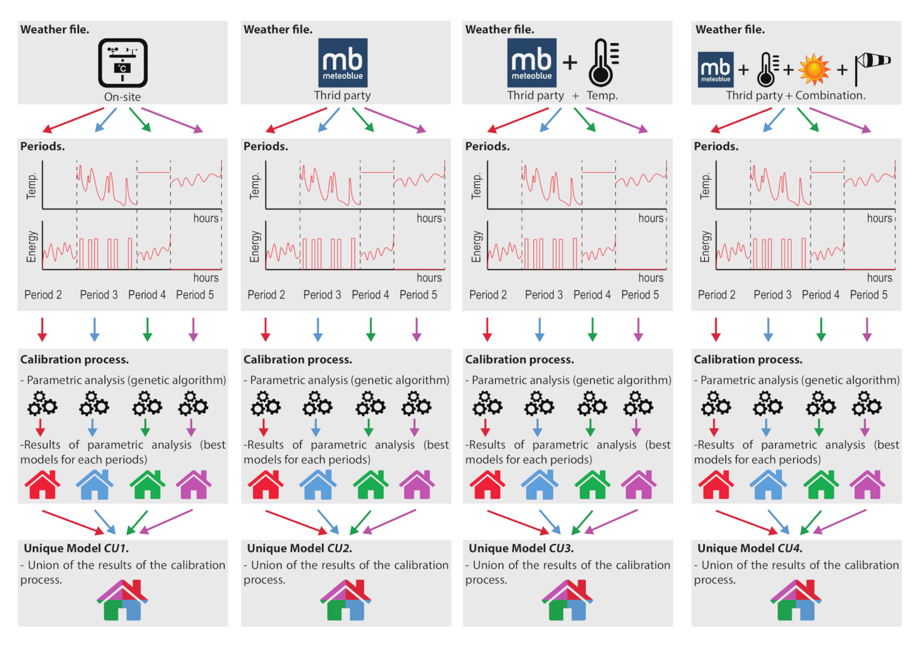
2. Design of the Method

To apply the methodology proposed in this paper, the data provided in annex 58 IEA-EBC [10,31] have been used both for the generation of the energy model and for obtaining the calibrated model.

We focused on the N2 house (N2 is the name of the house) in the German town of Holzkirchen near Munich. The house is situated on a flat area and there are no buildings in the vicinity to provide shade in the summer season when the annex was tested. The house has three floors (basement, ground floor, and attic) with a free height of 2.50 m. The test proposed by the annex focuses on the ground floor spaces: the two bedrooms, the living room, the entrance, the bathroom, the corridor and the kitchen (Figure 1). This housing is optimal for the realization of the proposed study because it provides all the necessary data for the accomplishment of the work. At the same time, these data are of a high quality, which reduces the uncertainty that they may cause in the final results of the research.

We focus on house N2 (N2 is the name of the house) in the German town of Holzkirchen, about 35 km south of Munich (47.874 N, 11.728 E). It is a house situated on a flat area without any buildings that could cast shadows on it in the summer period, which was the period of analysis. It shares the typical climate of Central Europe: oceanic. The house has three floors (basement, ground floor and attic) with a clear height of 2.50 m. The study focused on the ground floor. The study focused on the ground floor, which included a living room, a kitchen, an entrance, a bathroom, a corridor and two bedrooms (Figure 1). This dwelling is optimal for the proposed study because it provides all the data necessary to carry out the work. At the same time, this data is of high quality, which reduces the uncertainty it may cause in the final results of the research.

The exercise developed in annex 58 consisted of five periods of energization of the housing, each period with certain characteristics. The energy model then responds to reality, both in the energy consumed and in the temperature reached. The offered periods began with the first (initialization) duration of three days, where a constant interior temperature was maintained in the house at 30 °C. In period number 2 (Period 2, set point 30 °C), seven days in length, a constant temperature was still maintained at 30 °C inside the house, and the calibrated energy model provided the real energy consumed. In the 3rd period that lasted 14 days (Period 3, ROLBS), energy was introduced through the living room radiator in aleatory periods with a randomly ordered logarithmic binary sequence (ROLBS).

Within the EC COMPASS project [32], this sequence was developed. Its objective is to ensure that all relevant frequencies that can occur in a given time have the same weight. To achieve this, the on and off periods are chosen in logarithmically equal intervals and mixed in a quasi-random order. With this sequence, it can be ensured that there is no connection between solar gains and heat input through the HVAC systems. The energy model must be able to reproduce the internal temperature that this energy produces. In period 4 (Period 4, set point 25 °C), a constant temperature was again introduced into the house, but this time at 25 °C and the energy model reproduced the energy produced by that indoor temperature. The last period is the 5th (Period 5, free oscillation), where the house was left in free oscillation, i.e., without any energy contribution. The calibrated model, then, reproduced the interior temperatures.

For the weather files used in this exercise, a climate file offered by third parties was selected, located about 440 m in a straight line from the selected house (47.87 N, 11.73 E) and together with the data from the weather station placed on the site, a composition of the sensors was made (Table 1). Using the sensors of the on-site station as a basis, the sensors will be replaced by those of third parties, generating a total of 64 climate files. The sensors used were the outside temperature (T), global horizontal irradiation (GHI), diffuse horizontal irradiation (DHI), wind speed (WS), wind direction (WD), and relative humidity (RH).

Once the energy model of the house was created (baseline model), and having already generated the weather files that will be used in the test, we proceeded to simulate the energy model in all periods and with all the climate files, to obtain a list with the behavior of the weather files and, thereby, obtain which one is the best suited to reality.

The next step was to check that the simulations performed with all the weather files and the base model conformed to a fitting process, i.e., to subject the model to a calibration process. This process was conducted with 4 of the 64 climate archives generated. The four that were considered to be the most relevant were selected. These were:

The weather file produced by the weather station placed on site (on-site weather file). This climate file was chosen because it allegedly best represents the weather of the area.
Third-party weather file (third-party weather file). This file was selected as the alternative to the site’s weather station.
The weather file composed of the third-party, but replacing the outside temperature sensor with that of the site’s weather station (third-party weather file + on-site temperature sensor). This climate file was selected for being one of the most cost-effective.
The weather file that provided the best results in the simulations with the base model (weather file combination). This was chosen for being the one with the best results of adjustment with reality.

The research method used started with the selection of the weather files. Once they had been selected, the process of calibrating the base model began [9]. The objective of this procedure was to justify the impact that the weather files had on the calibrated model, thus checking which was the energy model that together with its weather file best fit reality and to verify that the ranking generated in the simulations of the base model with all the weather files was fulfilled (Figure 2).

The calibration process, tested in previous studies with different buildings and with satisfactory results, will generate the model that best fits in temperature and energy to all the periods proposed by the exercise in the annex (periods 2 to 5). To achieve this, several scripts were programmed in the EnergyPlus [33] run-time language. These commands transfer the measured temperature or energy to the model. The periods described in the previous paragraphs were also subjected to the calibration process shown in Figure 3. Although the methodology may resemble an optimization process, the objective function links the fit between the values provided by the model and the real data. In this case, the coefficient of variation of the root mean square error (CV(RMSE)) and the square Pearson correlation coefficient (

R^{2}

) were used [16]. To find the best solution, the non-dominant sorting genetic algorithm (NSGA-II) [34] was chosen as the search engine. The possible combinations of the parameters are those that will determine the search space, these are: thermal bridges, thermal mass, infiltrations and capacitances.

Once all the periods were calibrated according to this methodology, the model that best suited all of them was obtained. This calibration operation was then repeated with the proposed weather files.

When the calibrated models (CUi, …, CUn) were obtained, the adjustment they achieved with respect to the real temperature and energy were studied, thus discovering which was the weather file that after a calibration process of the energy model, was the closest to reality. In addition, we checked whether the adjustment classification of the base model with all the weather files had similarity with the results obtained in the calibrated models. The evaluation of the models was proposed to be performed with two types of indexes, the same ones that the genetic algorithm used in the calibration process: First, the CV(RMSE) (Equation (1)) which is the coefficient of variation of the root mean square error. The CV(RMSE) is achieved by weighting the Root Mean Square Error (RMSE) by the mean of the actual data. The measured variability is considered to be error variance by this index and therefore the American Society of Heating, Refrigerating, and Air Conditioning Engineers (ASHRAE) Guideline 14, the Federal Energy Management Program (FEMP) and the International Performance Maintenance and Verification Protocol (IPMVP) recommend its use [30,35,36,37,38,39,40,41,42]. Secondly, the coefficient of determination R

^{2}

(Equation (2)) which is the percentage of variation of the response variable that explains its relationship with one or more predictor variables. Generally, the higher the R

^{2}

, the better the fit of the model to its data. The R

^{2}

is always between 0 and 100%.

CV (R M S E) = \frac{1}{\bar{y}} {[\frac{\sum_{i = 1}^{n} {(y_{i} - {\hat{y}}_{i})}^{2}}{n - p}]}^{\frac{1}{2}}

(1)

R^{2} = {(\frac{\sum_{i = 1}^{n} (y_{i} - \bar{y}) ({\hat{y}}_{i} - \bar{\hat{y}})}{\sqrt{(\sum_{i = 1}^{n} {(y_{i} - \bar{y})}^{2}) (\sum_{i = 1}^{n} {({\hat{y}}_{i} - \bar{\hat{y}})}^{2})}})}^{2} .

(2)

3. Analysis of the Results and Discussion

The first exercise that was performed for the demonstration of the methodology was the simulation of the base model with all the proposed weather file combinations. This was an attempt to discover which climate file, by simulating it with a baseline model, best fit reality. The results can be seen in Figure 4 and Figure 5. Through the box plots, the results obtained in this phase of the methodology are shown. In both figures are highlighted the results of:

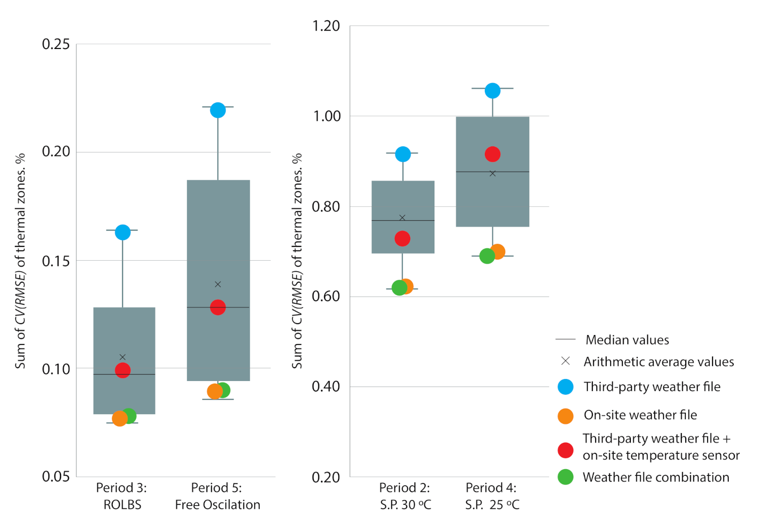
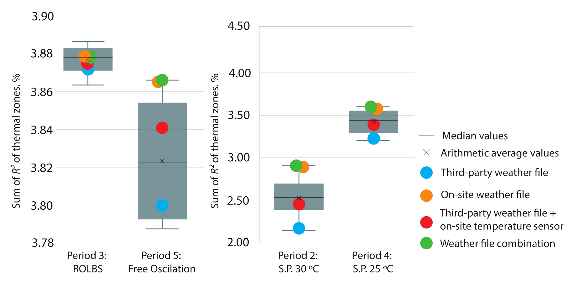
The weather file that best fit the real data, created from the combination of sensors from the weather station placed on site and the one obtained from third parties: “Weather file combination”. This configuration was: the wind speed, global, and diffuse horizontal irradiation and temperature sensors of the weather station placed on site and the wind direction and relative humidity sensors of the third-party. This is highlighted by a green circle in the figures.
The “third-party weather file + on-site temperature sensor”, created by adding, to the third-party climate file, the temperature sensor data from the site’s weather station. This is highlighted in the figures by a red circle. This weather file is one of the most cost-effective.
The weather file resulting from the sensors of the weather station placed at the site, “on-site weather file”. This is highlighted with an orange circle on the figures.
The meteorological file created with the third-party sensors “third-party weather file”. This is marked in blue in the figures.

Figure 4 shows the sum of the CV(RMSE) index of the thermal zones that come into play in the simulation (living room, bedroom, kitchen, and children’s room). This index has a range from 0 to ∞, where 0 represents the model with the best adjustment. This was obtained by comparing the temperature and energy data (depending on the period) generated by the base energy model and the different weather files with those of reality. Each period has its own box plot. On the left of the figure are the periods where the model is asked for temperature, and on the right are the periods where the model is asked for energy:

The required temperature periods for the energy model:

Period 3: During the 2 weeks that period 3 lasts, the house underwent an injection of energy through a ROLBS sequence, and the model was used to discover the temperature that this energy produces. Once the model with the different weather files was subjected to this period, we see that the weather file that behaved best was the “on-site weather file” and, almost in the same position, was the “weather file combination” both in quartile 1. The “third-party weather file + on-site temp. sensor” was at the limit of quartile 2 and 3, worsening the results with respect to period 2. Finally, the “third-party weather file” was still the worst performer at the upper limit of quartile 4.
Period 5: In this period, the house was in free oscillation and the model represented the temperatures that were obtained when no energy was injected into the house. The behavior of the weather files in this period had a similarity with the results obtained in period 3. Quartile 1 contained both the “weather file combination” and the “on-site weather file”. The latter was placed in the first position. Between quartile 2 and 3, there was the “third-party weather file + on-site temp. sensor”, which was almost at the average of the results. Finally, as in all other periods, the “third-party weather file” was placed on the upper edge of quartile 4.

Required energy periods to the energy model:

Period 2: In this period, the house was subjected to a constant temperature at 30 °C, and the energy model was required to be able to reproduce the energy needed to reach that temperature. The weather file that produced the best fit with reality was the “weather file combination” followed very closely by the on-site weather file, both located in the first quartile. Already in the second quartile, but above average, the “third-party weather file + on-site temp. sensor” was placed. The weather file that was the worst suited to reality is that of third parties, which is in the fourth quartile.
Period 4: The house was heated to 25 C and the energy model was able to reproduce the energy necessary to obtain that temperature. The best weather file was again the “weather combination”, this time making more of a difference to the “weather on-site”, although both files were in the first quartile. In the 3rd, below the average, we find the “third-party weather file + on-site temp. sensor” and, as in the other periods, located at a great distance from the rest. In the 4th quartile was the “third-party weather file”.

Figure 5 shows the sum of the index R

^{2}

of the thermal zones that enter the simulation process: living room, bedroom, kitchen, and children’s room. This index measures how much the shapes of the two curves resemble each other. In this case, the temperature and energy curves produced by the simulated model and the different weather files were compared with reality. The range was from 0 to 4 (4 because this is the sum of the four thermal zones that are analyzed in the energy model) with 4 being the model with the best adjustment. Each period is shown in a box plot. As in Figure 4, on the left are the periods where the model is asked for temperature, and on the right are the periods where the model is asked for energy.

The required temperature periods for the energy model:

Period 3: In this period, all the weather archives were much closer to each other. Even so, the one that best fit the reality was the “on-site weather file” in quartile 2, followed very closely by the “weather file combination”. Both files were above average. In third position was the “third-party weather file + on-site temperature sensor” located in quartile 3 below the average. The last position was the “third-party weather file” on the border between quartile 3 and 4.
Period 5: In this period, the difference in the results of the different weather data archives was greater. In quartile 1, the “weather file combination” was the best suited to reality. Next was the “on-site weather file”. In quartile 2 and above, but at a considerable distance, was the “third-party weather file + on-site temperature sensor”. In the last position, but in quartile 3, was the “third-party weather file”.

The required energy periods for the energy model:

Period 2: The “weather file combination” achieved the first position; this was the one that best fit the real data of the studied meteorological archives. This was in the first quartile followed very closely by the “on-site weather file”. In the third one was the “third-party weather file + on-site temp sensor” located a little behind the average. At the bottom of the fourth quartile, we find the “third-party weather file”.
Period 4: The weather file that best matched reality was the “weather file combination” located in quartile 1, as well as the “on-site weather file” that followed it very narrowly. The “third-party weather file + on-site temperature sensor” was in the third lower quartile. Finally, at the bottom edge of quartile 4 is the “third-party weather file”.

As a summary of the comments on the results of this analysis, the weather file that best fit the real data was the “weather file combination” followed at a very short distance by the “on-site weather file”. Thirdly, the “third-party weather file + on-site temperature sensor” was clearly positioned most of the time in the third quartile, but above average. For the “third-party weather file”, there is no doubt that it was the weather file that fit the worst to reality, placing itself, in most periods, in the lower limit of the last quartile.

Once this check was performed, the combination of sensors between those placed on site and those obtained from a third-party weather file were known to produce better adjustment results. This is the wind speed (WS), global (GHI) and diffuse (DHI) horizontal irradiation, and temperature (T) sensors of the weather station placed on the site and the wind direction (WD) and relative humidity (RH) sensors of the third-party.

The next step, as explained in the description of the methodology, is to justify the selection of the four weather files with which the calibration process was performed. They were:

The weather file that produced the best adjustment to real data when simulated with the base energy model: “weather file combination”.
The climate file with the best ratio between cost and effectiveness: “third-party weather file + on-site temperature sensor”.
The weather file created from sensor data from the on-site weather station: “On -site weather file”.
The weather file generated from sensor data gathered from third parties: “third-party weather file”.

The energy model with each type of weather file was subjected to a fitting process (explained in Section 2), with the aim of verifying whether the same results are obtained as in the classification made with the simulations of the baseline model and all the weather files (Figure 6).

The model with the four selected weather files was calibrated in each of the periods proposed in annex 58. The four calibrated models obtained for each period were joined into one, creating the model that best fits the reality in all periods. Thus, we obtained four calibrated models, one for each selected weather file:

CU1 model obtained with the “on -site weather file”.
CU2 model obtained with the “third-party weather file”.
CU3 model obtained with the “third-party weather file + on-site temperature sensor”.
CU4 model obtained with the “weather file combination”.

To present the results obtained, Table 2 was created to show the uncertainty indexes CV(RMSE) and R

^{2}

attained by the models in the different calibration periods. For the periods where the temperature generated by the energy model was compared with the real temperature, the area-weighted average of each thermal zone analyzed was considered to produce the index result. However, in the periods where the energy consumed is the comparison, the sum of the energy spent per thermal zone was carried out to achieve the uncertainty index.

To combine the effects on the weather file in all calibration periods in a unique result, the value of the temperature and energy indices obtained (normalized indices) was normalized, so that they have the same basis to be able to add them up and thus obtain a unified value (sum indices).

When studying the results obtained, the weather file that obtained the best results was the “weather file combination”, with an index sum value of 0.416, exceeding, by a very small margin, the “on-site weather file” (0.544). In third position was the “third-party weather file + on-site temperature sensor” with a normalized index sum value of 0.985. In addition, the “third-party weather file” obtained a normalized index sum value of 6.245, which was well behind the other weather files. As can be seen in the table, we confirmed that the ranking the weather files produced with the base model was repeated in the calibration process.

When analyzed in more detail, we concluded that in the periods where the result sought was temperature (period 3 and 5), both the “weather file combination”, “on-site weather file” and “third-party weather file + on-site temperature sensor”, had very similar results, all obtaining very good values. The biggest differences occurred when we examined the energy periods (periods 2 and 4). Here, the “weather file combination” and the “on-site weather file” produced a difference compared with the other files.

In addition, in period 4, the “weather file combination” was much better adjusted to the expected result of 8.08% CV(RMSE) compared to the 14.46% obtained by the “on-site weather file”.

Another analysis made to the weather archives was to determine if they complied with the objectives proposed by the international standards: The International Performance Measurement and Verification Protocol (IPMVP) determines that a model achieves best fit values when it manages to obtain a CV(RMSE) of less than

\pm 20 %

on an hourly scale. On the other hand, ASHRAE and the Federal Energy Management Program (FEMP) state that a model can be considered to be fit when it obtains a CV(RMSE) index of less than

\pm 30 %

on the same scale (Table 3). As for the R

^{2}

index, ASHRAE recommends that models should not have an index of less than

75 %

to be considered calibrated.

In Table 2, the results that are not colored comply with international standards, the results that comply with ASHRAE and FEMP have been colored in orange, while the periods that do not comply with any standard have been marked in red. Both the “weather file combination” and the “on-site weather file” met the standard expectations in all the periods analyzed. The “third-party weather file + on-site temperature sensor” achieved very good rates, although, in period 4, it did not manage to comply with the IPMVP standard in the CV(RMSE) rate value where it stayed with 20.60% being the limit to be able to comply with 20.00%. The “third-party weather file” failed to respond satisfactorily in period 2, where it did not meet the value of R

^{2}

, and in period 4 where it did not reach a good value for either index.

4. Conclusions

Based on the results obtained with the study conducted in this paper, a new method is proposed to establish the degree to which the sensors that generate the climate file were affected in the process of adjusting the energy models of the building. Thus, we were able to select the best composition of sensors depending on the needs of the project.

Different types of sensors come into play in the process of creating the weather file: the wind speed and direction, global and diffuse horizontal irradiation, the outdoor temperature, and the relative humidity. Data from these sensors can be obtained from weather stations placed at the experiment site or can be acquired from third parties.

A weather station placed on the site requires a strong economic investment not only when buying or renting the group of sensors needed, as well as when processing and validating the data generated. Although weather data acquired from third parties are much cheaper, they have the disadvantage of being less accurate.

In this article, a new fast methodology was developed to determine the degree of adjustment of the different weather files composed of site data and third-party data. To this end, the sensors of the on-site weather station and those of third parties were combined with the aim of creating as many climate files as possible, resulting in a total of sixty-four files.

The results obtained in the experiment confirmed that there was a combination of sensors that offered a better degree of adjustment between the simulated temperatures and energies and reality than those offered by the site’s weather station. Using these sensors to compose the weather file allowed the energy model to represent reality more accurately. This combination used the wind speed (WS), global and diffuse solar radiation (GHI), and temperature (T) sensors from the weather station placed at the site and the wind direction (WD) and relative humidity (RH) sensors from the data provided by third parties (weather file combination).

Good results were obtained by the climate file composed of the third-party data plus the temperature sensor of the site’s weather station (third-party + on-site temp. sensor). With a very low economic cost, as it was simply necessary to place a temperature sensor outside the building, very positive adjustment results were achieved. The model behaved with excellent performance in all periods, complying with the parameters proposed by ASHRAE both in the CV(RMSE) and in R

^{2}

index. This model obtained a normalized index sum of 0.985 compared to 0.544 as obtained by the model calibrated with the site’s climate file. This is a difference to be considered, but is far from the one that occurs with the model adjusted with the climate file composed of third-party data, which obtained an index sum of 6.245. Depending on the degree of precision that must be obtained in the energy model, this option can be a good way to deal with the adjustment process. The weather file had the best cost-effectiveness ratio.

One of the most relevant conclusions obtained when developing the proposed methodology was the fact that it was not necessary to go through a process of adjustment of the model to be able to indicate the effect of the weather file in the final result. The results obtained when simulating all the proposed climate archives with the base model were the same as those obtained when executing an adjustment process. Even the positions in which the files were placed, as well as the distance between them, were met.

With the methodology proposed here, in a swift and simple way, we opened the option of being able to choose the composition of the meteorological file for use in the energy model adjustment process. This decision can be considered for economic, precision, and effectiveness factors, among others.

Author Contributions

V.G.G. and C.F.B. supervised the methodology used in the article, performed the simulations and the analysis, and wrote the manuscript. G.R.R. developed the EnergyPlus model and participated in the data analysis. All authors have read and agreed to the published version of the manuscript.

Funding

The work was funded by the research and innovation program Horizon 2020 of the European Union under Grant No. 731211, project SABINA.

Acknowledgments

We would like to thank the promoters of annex 58, the possibility of accessing the data of the houses. Without this data it would not have been possible to complete this work.

Conflicts of Interest

The authors declare no conflict of interest.

Abbreviations

The following abbreviations are used in this manuscript:

BEM	Building Energy Model
CV(RMSE)	Coefficient of Variation of Mean Square Error
MPC	Model Predictive Control
R $^{2}$	Square Pearson Correlation Coefficient
FDD	Fault Detection Diagnosis
SABINA	SmArt BI-directional multi eNergy gAteway
P2H	Power to Heat
IEA-EBC	International Energy Agency Energy in Buildings and Communities
HVAC	Heating Ventilation Air Conditioning
ESCOs	Energy Service Companies
IPMVP	International Measurement a Verification Protocol
EU	European Union
WD	Wind Direction
C	Celsius degrees
WS	Wind Speed
m	Meter
N	North
E	East
T	Temperature
GHI	global radiation
WD	Wind Direction
RH	Relative Humidity
DHI	diffuse radiation
FEMP	Federal Energy Management Program
NSGA-II	Non-Dominated Sorting Genetic Algorithm
RMSE	Root Mean Square Error
ASHRAE	American Society of Heating, Refrigerating, and Air Conditioning Engineers
%	Percentage

References

Zhang, Z.; Chong, A.; Pan, Y.; Zhang, C.; Lam, K.P. Whole building energy model for HVAC optimal control: A practical framework based on deep reinforcement learning. Energy Build. 2019, 199, 472–490. [Google Scholar] [CrossRef]
Hensen, J.L.; Lamberts, R. Building Performance Simulation for Design and Operation; Routledge: London, UK, 2012. [Google Scholar]
SABINA H2020 EU Program. Available online: http://sindominio.net/ash (accessed on 10 June 2020).
Kohlhepp, P.; Hagenmeyer, V. Technical potential of buildings in Germany as flexible power-to-heat storage for smart-grid operation. Energy Technol. 2017, 5, 1084–1104. [Google Scholar] [CrossRef] [Green Version]
Bloess, A.; Schill, W.P.; Zerrahn, A. Power-to-heat for renewable energy integration: A review of technologies, modeling approaches, and flexibility potentials. Appl. Energy 2018, 212, 1611–1626. [Google Scholar] [CrossRef]
Fernández Bandera, C.; Pachano, J.; Salom, J.; Peppas, A.; Ramos Ruiz, G. Photovoltaic Plant Optimization to Leverage Electric Self Consumption by Harnessing Building Thermal Mass. Sustainability 2020, 12, 553. [Google Scholar] [CrossRef] [Green Version]
Ruiz, G.R.; Bandera, C.F.; Temes, T.G.A.; Gutierrez, A.S.O. Genetic algorithm for building envelope calibration. Appl. Energy 2016, 168, 691–705. [Google Scholar] [CrossRef]
Fernández Bandera, C.; Ramos Ruiz, G. Towards a new generation of building envelope calibration. Energies 2017, 10, 2102. [Google Scholar] [CrossRef] [Green Version]
González, V.G.; Ruiz, G.R.; Bandera, C.F. Empirical and Comparative Validation for a Building Energy Model Calibration Methodology. Sensors 2020, 20, 5003. [Google Scholar] [CrossRef]
Strachan, P.; Svehla, K.; Heusler, I.; Kersken, M. Whole model empirical validation on a full-scale building. J. Build. Perform. Simul. 2016, 9, 331–350. [Google Scholar] [CrossRef] [Green Version]
Agüera-Pérez, A.; Palomares-Salas, J.C.; de la Rosa, J.J.G.; Florencias-Oliveros, O. Weather forecasts for microgrid energy management: Review, discussion and recommendations. Appl. Energy 2018, 228, 265–278. [Google Scholar] [CrossRef]
González, V.G.; Ruiz, G.R.; Segarra, E.L.; Gordillo, G.C.; Bandera, C.F. Characterization of Building Foundation in Building Energy Models. In Proceedings of the Building Simulation, Rome, Italy, 2–4 September 2019. [Google Scholar]
United States Department of Energy. EnergyPlus Engineering Reference: The Reference to EnergyPlus Calculations; Lawrence Berkeley National Laboratory: Berkeley, CA, USA, 2009. [Google Scholar]
Coakley, D.; Raftery, P.; Keane, M. A review of methods to match building energy simulation models to measured data. Renew. Sustain. Energy Rev. 2014, 37, 123–141. [Google Scholar] [CrossRef] [Green Version]
Ruiz, G.R.; Bandera, C.F. Analysis of uncertainty indices used for building envelope calibration. Appl. Energy 2017, 185, 82–94. [Google Scholar] [CrossRef]
González, V.G.; Colmenares, L.Á.; Fidalgo, J.F.L.; Ruiz, G.R.; Bandera, C.F. Uncertainy’s Indices Assessment for Calibrated Energy Models. Energies 2019, 12, 2096. [Google Scholar] [CrossRef] [Green Version]
De Wit, S.; Augenbroe, G. Analysis of uncertainty in building design evaluations and its implications. Energy Build. 2002, 34, 951–958. [Google Scholar] [CrossRef]
Segarra, E.L.; Ruiz, G.R.; González, V.G.; Peppas, A.; Bandera, C.F. Impact Assessment for Building Energy Models Using Observed vs. Third-Party Weather Data Sets. Sustainability 2020, 12, 6788. [Google Scholar] [CrossRef]
Erba, S.; Causone, F.; Armani, R. The effect of weather datasets on building energy simulation outputs. Energy Procedia 2017, 134, 545–554. [Google Scholar] [CrossRef]
Voisin, J.; Darnon, M.; Jaouad, A.; Volatier, M.; Aimez, V.; Trovão, J.P. Climate impact analysis on the optimal sizing of a stand-alone hybrid building. Energy Build. 2020, 210, 109676. [Google Scholar] [CrossRef]
Bhandari, M.; Shrestha, S.; New, J. Evaluation of weather datasets for building energy simulation. Energy Build. 2012, 49, 109–118. [Google Scholar] [CrossRef]
Sandels, C.; Widén, J.; Nordström, L.; Andersson, E. Day-ahead predictions of electricity consumption in a Swedish office building from weather, occupancy, and temporal data. Energy Build. 2015, 108, 279–290. [Google Scholar] [CrossRef]
Du, H.; Barclay, M.; Jones, P. Generating high resolution near-future weather forecasts for urban scale building performance modelling. In Proceedings of the 15th Conference of International Building Performance Simulation Association, San Francisco, CA, USA, 7–9 August 2017. [Google Scholar]
Du, H.; Jones, P.; Segarra, E.L.; Bandera, C.F. Development of a REST API for obtaining site-specific historical and near-future weather data in EPW format. In Proceedings of the Building Simulation and Optimization 2018, Cambridge, UK, 11–12 September 2018. [Google Scholar]
Silvero, F.; Lops, C.; Montelpare, S.; Rodrigues, F. Generation and assessment of local climatic data from numerical meteorological codes for calibration of building energy models. Energy Build. 2019, 188, 25–45. [Google Scholar] [CrossRef]
Cuerda, E.; Guerra-Santin, O.; Sendra, J.J.; Neila, F.J. Understanding the performance gap in energy retrofitting: Measured input data for adjusting building simulation models. Energy Build. 2020, 209, 109688. [Google Scholar] [CrossRef]
Song, S.; Haberl, J.S. Analysis of the impact of using synthetic data correlated with measured data on the calibrated as-built simulation of a commercial building. Energy Build. 2013, 67, 97–107. [Google Scholar] [CrossRef]
Ciobanu, D.; Eftimie, E.; Jaliu, C. The influence of measured/simulated weather data on evaluating the energy need in buildings. Energy Procedia 2014, 48, 796–805. [Google Scholar] [CrossRef] [Green Version]
Afram, A.; Janabi-Sharifi, F. Theory and applications of HVAC control systems–A review of model predictive control (MPC). Build. Environ. 2014, 72, 343–355. [Google Scholar] [CrossRef]
Cowan, J. International Performance Measurement and Verification Protocol: Concepts and Options for Determining Energy and Water Savings-Vol. I. International Performance Measurement & Verification Protocol, 1. LBNL Report #: LBNL/PUB-909. Available online: https://escholarship.org/uc/item/68b7v8rd (accessed on 10 June 2020).
Annex 58: Reliable Building Energy Performance Characterisation Based on Full Scale Dynamic Measurement. 2016. Available online: https://bwk.kuleuven.be/bwf/projects/annex58/index.htm (accessed on 10 June 2020).
van Dijk, H.; Tellez, F. Measurement and Data Analysis Procedures, Final Report of the JOULE IICOMPASS project (JOU2-CT92-0216). 1995.
Crawley, D.B.; Hand, J.W.; Kummert, M.; Griffith, B.T. Contrasting the capabilities of building energy performance simulation programs. Build. Environ. 2008, 43, 661–673. [Google Scholar] [CrossRef] [Green Version]
Deb, K.; Pratap, A.; Agarwal, S.; Meyarivan, T. A fast and elitist multiobjective genetic algorithm: NSGA-II. IEEE Trans. Evol. Comput. 2002, 6, 182–197. [Google Scholar] [CrossRef] [Green Version]
Guideline, A. Measurement of Energy and Demand Savings; Guideline 14-2002; American Society of Heating, Ventilating, and Air Conditioning Engineers: Atlanta, GA, USA, 2002. [Google Scholar]
Lucas Segarra, E.; Du, H.; Ramos Ruiz, G.; Fernández Bandera, C. Methodology for the quantification of the impact of weather forecasts in predictive simulation models. Energies 2019, 12, 1309. [Google Scholar] [CrossRef] [Green Version]
Ruiz, G.R.; Bandera, C.F. Importancia del clima en la simulación energética de edificios. In Jornadas Internacionales de Investigación en Construcción: Vivienda: Pasado, Presente y Futuro: Resúmenes y Actas; Instituto Eduardo Torroja: Madrid, Spain, 2013. [Google Scholar]
Du, H.; Bandera, C.F.; Chen, L. Nowcasting methods for optimising building performance. In Proceedings of the Building Simulation 2019: 16th Conference of International Building Performance Simulation Association, Rome, Italy, 2–4 September 2019. [Google Scholar]
Li, H.; Hong, T.; Sofos, M. An inverse approach to solving zone air infiltration rate and people count using indoor environmental sensor data. Energy Build. 2019, 198, 228–242. [Google Scholar] [CrossRef] [Green Version]
Martínez, S.; Eguía, P.; Granada, E.; Moazami, A.; Hamdy, M. A performance comparison of multi-objective optimization-based approaches for calibrating white-box building energy models. Energy Build. 2020, 216, 109942. [Google Scholar] [CrossRef]
Reddy, T.A.; Maor, I.; Panjapornpon, C. Calibrating Detailed Building Energy Simulation Programs with Measured Data—Part I: General Methodology (RP-1051). HVAC&R Res. 2007, 13, 221–241. [Google Scholar] [CrossRef]
Carroll, W.; Hitchcock, R. Tuning simulated building descriptions to match actual utility data: Methods and implementation. ASHRAE Trans. Am. Soc. Heat. Refrig. Aircond. Eng. 1993, 99, 928–934. [Google Scholar]

Figure 1. Plan and external views of the N2 house. Holzkirchen, Germany.

Figure 2. Generic process diagram for achieving calibration mode.

Figure 3. Calibration environment with a genetic algorithm. The coefficient of variation of the root mean square error (CV(RMSE)) and the genetic algorithm non-dominated sorting genetic algorithm (NSGA-II) [9].

Figure 4. The simulation result of the base model with all the proposed weather files. CV(RMSE) Index.

Figure 5. The simulation result of the base model with all the proposed weather files. R

^{2}

Index.

Figure 5. The simulation result of the base model with all the proposed weather files. R

^{2}

Index.

Figure 6. The process diagram for achieving the calibrated model.

Table 1. All possible combinations of weather files. The sensors used were the outside temperature (T), global horizontal irradiation (GHI), diffuse horizontal irradiation (DHI), wind speed (WS), wind direction (WD), and relative humidity (RH).

Weather Combination				Weather Combination
Weather File Name	On-Site Weather Sensors	+	Third-Party Weather Sensors	Weather File Name	On-Site Weather Sensors	+	Third-Party Weather Sensors
Third-party	—	+	WS; WD; RH; GHI; DHI; T	Weather 33	WS	+	WD; RH; GHI; DHI; T
Weather 02	DHI	+	WS; WD; RH; GHI; T	Weather 34	WS; DHI	+	WD; RH; GHI; T
Weather 03	DHI; T	+	WS; WD; RH; GHI	Weather 35	WS; DHI; T	+	WD; RH; GHI
Weather 04	GHI	+	WS; WD; RH; DHI; T	Weather 36	WS; GHI	+	WD; RH; DHI; T
Weather 05	GHI; DHI	+	WS; WD; RH; T	Weather 37	WS; GHI; DHI	+	WD; RH; T
Weather 06	GHI; DHI; T	+	WS; WD; RH	Combination	WS; GHI; DHI; T	+	WD; RH
Weather 07	GHI; T	+	WS; WD; RH; DHI	Weather 39	WS; GHI; T	+	WD; RH; DHI
Weather 08	RH	+	WS; WD; GHI; DHI; T	Weather 40	WS; RH	+	WD; GHI; DHI; T
Weather 09	RH; DHI	+	WS; WD; GHI; T	Weather 41	WS; RH; DHI	+	WD; GHI; T
Weather 10	RH; DHI; T	+	WS; WD; GHI	Weather 42	WS; RH; DHI; T	+	WD; GHI; T
Weather 11	RH; GHI	+	WS; WD; DHI; T	Weather 43	WS; RH; GHI	+	WD; DHI; T
Weather 12	RH; GHI; DHI	+	WS; WD; T	Weather 44	WS; RH; GHI; DHI	+	WD; T
Weather 13	RH; GHI; DHI; T	+	WS; WD	Weather 45	WS; RH; GHI; DHI; T	+	WD
Weather 14	RH; GHI; T	+	WS; WD; DHI	Weather 46	WS; RH; GHI; T	+	WD; DHI
Weather 15	RH; T	+	WS; WD; GHI; DHI	Weather 47	WS; RH; T	+	WD; GHI; DHI
Third-party + On-site temp. sensor	T	+	WS; WD; RH GHI; DHI	Weather 48	WS; T	+	WD; RH; GHI; DHI
Weather 17	WD	+	WS; RH; GHI; DHI; T	Weather 49	WS; WD	+	RH; GHI; DHI; T
Weather 18	WD; DHI	+	WS; RH; GHI; T	Weather 50	WS; WD; DHI	+	RH; GHI; T
Weather 19	WD; DHI; T	+	WS; RH; GHI	Weather 51	WS; WD; DHI; T	+	RH; GHI
Weather 20	WD; GHI	+	WS; RH; DHI; T	Weather 52	WS; WD; GHI	+	RH; DHI; T
Weather 21	WD; GHI; DHI	+	WS; RH; T	Weather 53	WS; WD; GHI; DHI	+	RH; T
Weather 22	WD; GHI; DHI; T	+	WS; RH	Weather 54	WS; WD; GHI; DHI; T	+	RH
Weather 23	WD; GHI; T	+	WS; RH; DHI	Weather 55	WS; WD; GHI; T	+	RH; DHI
Weather 24	WD; RH	+	WS; DHI; GHI; T	Weather 56	WS; WD; RH	+	GHI; DHI; T
Weather 25	WD; RH; DHI	+	WS; GHI; T	Weather 57	WS; WD; RH; DHI	+	GHI; T
Weather 26	WD; RH; DHI; T	+	WS; GHI	Weather 58	WS; WD; RH; DHI; T	+	GHI
Weather 27	WD; RH; GHI	+	WS; DHI; T	Weather 59	WS; WD; RH; GHI	+	DHI; T
Weather 28	WD; RH; GHI; DHI	+	WS; T	Weather 60	WS; WD; RH; GHI; DHI	+	T
Weather 29	WD; RH; GHI; DHI; T	+	WS	On-site	WS; WD; RH; GHI; DHI; T	+	—
Weather 30	WD; RH; GHI; T	+	WS; DHI	Weather 62	WS; WD; RH; GHI; T	+	DHI
Weather 31	WD; RH; T	+	WS; GHI; DHI	Weather 63	WS; WD; RH; T	+	GHI; DHI
Weather 32	WD; T	+	WS; RH; GHI; DHI	Weather 64	WS; WD; T	+	RH; GHI; DHI

Table 2. The normalized results in the checking periods with the different weather files. Randomly ordered logarithmic binary sequence (ROLBS).

Weather	Model	Checking Period	Index		Normalized Indices	Indices Sum
				Average house
				temperatures
		Period 3 (ROLBS)	CV(RMSE)	1.23%	0.000
			R $^{2}$	99.07%	0.000
		Period 5 (Free oscillation)	CV(RMSE)	1.63%	0.109
			R $^{2}$	98.66%	0.021
On-site	Model
	CU1			Sum of
				housing energy
		Period 2 (Set point 30 C)	CV(RMSE)	9.65%	0.049
			R $^{2}$	91.80%	0.091
		Period 4 (Set point 25 C)	CV(RMSE)	14.46%	0.200
			R $^{2}$	92.77%	0.072	0.544
				Average house
				temperatures
		Period 3 (ROLBS)	CV(RMSE)	4.87%	1.000
			R $^{2}$	90.26%	0.453
		Period 5 (Free oscillation)	CV(RMSE)	4.70%	0.953
			R $^{2}$	79.62%	1.000
Third-party	Model
	CU2			Sum of
				housing energy
		Period 2 (Set point 30 C)	CV(RMSE)	17.84%	0.307
			R $^{2}$	69.66%	0.532
		Period 4 (Set point 25 C)	CV(RMSE)	39.93%	1.000
			R $^{2}$	46.20%	1.000	6.245
				Average house
				temperatures
		Period 3 (ROLBS)	CV(RMSE)	1.33%	0.026
			R $^{2}$	98.75%	0.017
		Period 5 (Free oscillation)	CV(RMSE)	1.45%	0.059
			R $^{2}$	98.55%	0.027
Third-party +	Model
Temp.	CU3			Sum of
				housing energy
		Period 2 (Set point 30 C)	CV(RMSE)	12.53%	0.140
			R $^{2}$	88.47%	0.157
		Period 4 (Set point 25 C)	CV(RMSE)	20.60%	0.393
			R $^{2}$	88.09%	0.165	0.985
				Average house
				temperatures
		Period 3 (ROLBS)	CV(RMSE)	1.37%	0.039
			R $^{2}$	98.87%	0.011
		Period 5 (Free oscillation)	CV(RMSE)	1.68%	0.123
			R $^{2}$	98.21%	0.044
Combination	Model
	CU4			Sum of
				housing energy
		Period 2 (Set point 30 C)	CV(RMSE)	11.16%	0.097
			R $^{2}$	91.22%	0.103
		Period 4 (Set point 25 C)	CV(RMSE)	8.08%	0.000
			R $^{2}$	96.37%	0.000	0.416

Table 3. The calibration criteria of Federal Energy Management Program (FEMP), American Society of Heating, Refrigerating, and Air Conditioning Engineers (ASHRAE), and international performance measurement and verification protocol (IPMVP).

Data Type	Index	FEMP 3.0 Criteria	ASHRAE G14-2002	IPMVP
Calibration Criteria
Monthly Criteria %	CV(RMSE)	$\pm 15$	$\pm 15$	-
Hourly Criteria %	CV(RMSE)	$\pm 30$	$\pm 30$	$\pm 20$

Publisher’s Note: MDPI stays neutral with regard to jurisdictional claims in published maps and institutional affiliations.

© 2021 by the authors. Licensee MDPI, Basel, Switzerland. This article is an open access article distributed under the terms and conditions of the Creative Commons Attribution (CC BY) license (http://creativecommons.org/licenses/by/4.0/).

Share and Cite

MDPI and ACS Style

Gutiérrez González, V.; Ramos Ruiz, G.; Fernández Bandera, C. Impact of Actual Weather Datasets for Calibrating White-Box Building Energy Models Base on Monitored Data. Energies 2021, 14, 1187. https://0-doi-org.brum.beds.ac.uk/10.3390/en14041187

AMA Style

Gutiérrez González V, Ramos Ruiz G, Fernández Bandera C. Impact of Actual Weather Datasets for Calibrating White-Box Building Energy Models Base on Monitored Data. Energies. 2021; 14(4):1187. https://0-doi-org.brum.beds.ac.uk/10.3390/en14041187

Chicago/Turabian Style

Gutiérrez González, Vicente, Germán Ramos Ruiz, and Carlos Fernández Bandera. 2021. "Impact of Actual Weather Datasets for Calibrating White-Box Building Energy Models Base on Monitored Data" Energies 14, no. 4: 1187. https://0-doi-org.brum.beds.ac.uk/10.3390/en14041187

Note that from the first issue of 2016, this journal uses article numbers instead of page numbers. See further details here.

Article Menu

Impact of Actual Weather Datasets for Calibrating White-Box Building Energy Models Base on Monitored Data

Abstract

1. Introduction

2. Design of the Method

3. Analysis of the Results and Discussion

4. Conclusions

Author Contributions

Funding

Acknowledgments

Conflicts of Interest

Abbreviations

References

Share and Cite

Article Metrics

Article Access Statistics

Further Information

Guidelines

MDPI Initiatives

Follow MDPI