
Double-Target Based Neural Networks in Predicting Energy Consumption in Residential Buildings


1
Institute of Research and Development, Duy Tan University, Da Nang 550000, Vietnam
2
Faculty of Civil Engineering, Duy Tan University, Da Nang 550000, Vietnam
3
Faculty of Civil Engineering, Technische Universität Dresden, 01069 Dresden, Germany
4
School of Economics and Business, Norwegian University of Life Sciences, 1430 Ås, Norway
5
John von Neumann Faculty of Informatics, Obuda University, 1034 Budapest, Hungary
6
School of the Built Environment, Oxford Brookes University, Oxford OX3 0BP, UK
*
Author to whom correspondence should be addressed.
Energies 2021, 14(5), 1331; https://0-doi-org.brum.beds.ac.uk/10.3390/en14051331
Submission received: 5 January 2021
/
Revised: 21 February 2021
/
Accepted: 22 February 2021
/
Published: 1 March 2021
(This article belongs to the Special Issue Smart Built Environment for Health and Comfort with Energy Efficiency)
Abstract
:A reliable prediction of sustainable energy consumption is key for designing environmentally friendly buildings. In this study, three novel hybrid intelligent methods, namely the grasshopper optimization algorithm (GOA), wind-driven optimization (WDO), and biogeography-based optimization (BBO), are employed to optimize the multitarget prediction of heating loads (HLs) and cooling loads (CLs) in the heating, ventilation and air conditioning (HVAC) systems. Concerning the optimization of the applied algorithms, a series of swarm-based iterations are performed, and the best structure is proposed for each model. The GOA, WDO, and BBO algorithms are mixed with a class of feedforward artificial neural networks (ANNs), which is called a multi-layer perceptron (MLP) to predict the HL and CL. According to the sensitivity analysis, the WDO with swarm size = 500 proposes the most-fitted ANN. The proposed WDO-ANN provided an accurate prediction in terms of heating load (training (R2 correlation = 0.977 and RMSE error = 0.183) and testing (R2 correlation = 0.973 and RMSE error = 0.190)) and yielded the best-fitted prediction in terms of cooling load (training (R2 correlation = 0.99 and RMSE error = 0.147) and testing (R2 correlation = 0.99 and RMSE error = 0.148)).
1. Introduction
The concerns about reducing energy consumption in smart cities are growing. Indeed, the rate of energy consumption has risen mainly in the last two decades. For instance, in buildings, an approximate increasing rate of consumption of 0.9% per year in the USA was reported by the US Energy Information Administration (EIA) [1]. In this regard, the residential buildings (as it is the main concern of the present study) consume approximately 38% of electricity energy. Therefore, almost one-fourth of the world’s energy is consumed in residential buildings [2]. Considering climate change, environmental concerns, as well as an overall significant contribution of buildings and their high demands on the consumption of such energy use, new intelligent methods are required to reduce this energy consumption. The rate of energy consumption of buildings has been investigated by various researchers such as Zhou, et al. [3], Ahmad, et al. [4], and Mocanu, et al. [5].
1.1. Background of Artificial Intelligence
With recent advances in computational intelligence, many scholars have replaced traditional methods with new generated machine learning [6,7,8,9,10,11], deep learning [12,13,14,15,16,17], decision making [18,19], and artificial intelligence-based tools [20,21,22]. These novel approximation techniques are well employed in various engineering fields such as in evaluating environmental concerns [19,23,24,25,26,27,28,29,30,31], implications for natural environmental management [32,33,34,35,36,37,38,39], water resources management [28,40,41,42,43,44], natural gas consumption [45,46,47,48], energy efficiency [49,50,51,52,53,54,55,56], image processing [57,58,59], building construction and design [60,61,62], feature selection/extraction [63,64,65,66,67], face recognition [68,69], climate change [70], managing smart cities [71], and project management [72], while in the field of medical science artificial intelligence is employed to have a better diagnosis of particular patients [41,73,74,75], early diagnosis of them [76], or medical image classification [77]. There have been many novel algorithms enhancing the current predictive neural network-based models. Metaheuristic algorithms have been highly regarded in various problems that demand an optimal solution [78]. The hybrid optimization techniques such as differential evolution [79], data-driven robust optimization [80], the whale optimization algorithm [81,82], harris hawks optimization [83], the differential edge detection algorithm [84], many-objective sizing optimizations [85], fruit fly optimization [86], the moth-flame optimization strategy [87], bacterial foraging optimization [88], ant colony optimization [89], particle swarm optimization (PSO) [90,91,92], chaos enhanced grey wolf optimization [73], and quantum-enhanced multiobjective large-scale [93].
Zhou, et al. [3] applied a feedforward artificial neural network (ANN) combined with a hybrid system (for example, considering the multivariable optimization process). The results obtained from their study showed that the generated ANN-based data-driven training algorithm is more reliable than the traditional “lsqcurvefit” fitting method. Asadi, et al. [94] investigated the energy consumption prediction of the building retrofits. They used a combination of the ANN and a genetic algorithm to find the most proper structure of a hybrid algorithm and to assess the interaction among conflicting objectives. Mocanu, et al. [5] stated that the deep learning-based solution methods are aimed to enhance the estimation level of the predictive network by letting a higher level of abstraction be implemented. Ahmad, et al. [4] stated that the management of energy-efficient buildings and predicting energy consumption for all buildings are critical tasks for decision-makers, in order to save effective energy as well as to develop smart cities. They reviewed some of the employed prediction techniques in estimating the building electrical energy using the most updated artificial intelligence (AI)-based solution. Zhou, et al. [3] investigated the use of a new hybrid system combined with active cooling, phase change materials, and hybrid ventilations.
1.2. HL and CL-Related Studies
Many researchers also have aimed to investigate the links between the heating loads (HLs) and cooling loads (CLs) and their most influential parameters such as the speed of the wind, the conditions of the environment climate changing, the rate of light, etc. Budaiwi and Abdou [95] successfully employed the heating, ventilation, and air conditioning (HVAC) system operational strategies to deduce the amount of consumed energy in buildings. In their study, they used an example of buildings with intermittent occupancy. Nasruddin, et al. [96] studied the HVAC optimization system to measure energy consumption in a particular building dataset. They used ANN as well as a multi-objective GA. Their findings provided possible design variables that can help to achieve the best-fit HVAC system. The results proved to be practical in terms of both annual energy consumption and thermal comfort. Min, et al. [97] explored indirect evaporative cooling energy recovery systems (for example, to pursue a high-quality indoor thermal environment) through a new statistical modeling approach. The validation of the proposed model was done using a series of experimental data. Roy, et al. [98] predicted heating load in buildings by employing a hybrid model of multivariate adaptive regression splines (MARS) and extreme learning machine (ELM). Liu, et al. [99] studied hierarchical modeling and temperature interval techniques to optimize the prediction of a multi-layer hybrid building’s cooling and heating load. The obtained results are compared with the basic estimation models, showing that the accuracy of the proposed models is significantly enhanced [99]. Kavaklioglu [100] proposed a new rebuts modeling of cooling and heating loads to have an efficient residential building design. Moayedi, et al. [101] investigated the social behavior of elephant herds in order to predict cooling load of residential buildings. In this sense, the technique of elephant herding optimization (EHO) is employed to optimize the trend of the HVAC system. In the other study, the k-fold cross-validation method was used to validate the proposed hybrid models, as discussed by Qiao, et al. [102]. Conventional modeling such as ordinary least squares was employed to have a better comparison between the obtained results and traditional techniques. The results showed that the developed methods are excellent in providing links between the influential factors and the target, which were heating and cooling loads.
1.3. Novelty and Proposed Methods
Based on the applicability of metaheuristic algorithms for a wide range of optimization techniques (for example, [13,93,103,104,105,106,107,108,109,110,111]), this study is particularly conducted in the case of thermal load analysis for residential buildings, where their real operations highly rely on building design criteria. The building design codes try to reduce the amount of energy consumption by considering two key terms: CLs and HLs. The HVAC is a well-known technology for indoor and vehicular environmental comfort. The concept of HVAC is a key issue in designing residential building structures such as apartment buildings, hotels, family homes, senior living facilities, office and industrial buildings (for example, medium to large), hospitals, and skyscrapers. Indeed, the subject of HAVC is not limited to building only, and it can be considered for the commonly used vehicles such as trains, cars, airplanes, large ships as well as submarines that work in the marine environments. The main objective of the HVAC system is to provide acceptable indoor air quality and thermal comfort. Although there are many new techniques to calculate HLs and CLs, there is still a lack of proper intelligence techniques in the prediction of these parameters. Studying through the current literature, numerous studies have used popular optimization methods [112,113] but the lack of multiobjective consideration of both HL and CL as well as more up-to-date hybrid intelligent-based solutions can be a suitable gap of knowledge in the subject of HVAC systems simulation. Therefore, this article recommends three novel multiobjective intelligent-based solutions on the herding trend of the grasshopper optimization algorithm (GOA), wind-driven optimization (WDO), and biogeography-based optimization (BBO) to predict the multi targets of HLs and CLs of residential buildings. These algorithms enhance the current ANN-based solutions. In this regard, over 33,000 model iterations are performed to provide the best-fit structure of combined algorithms.
2. Methodology and Theoretical Background
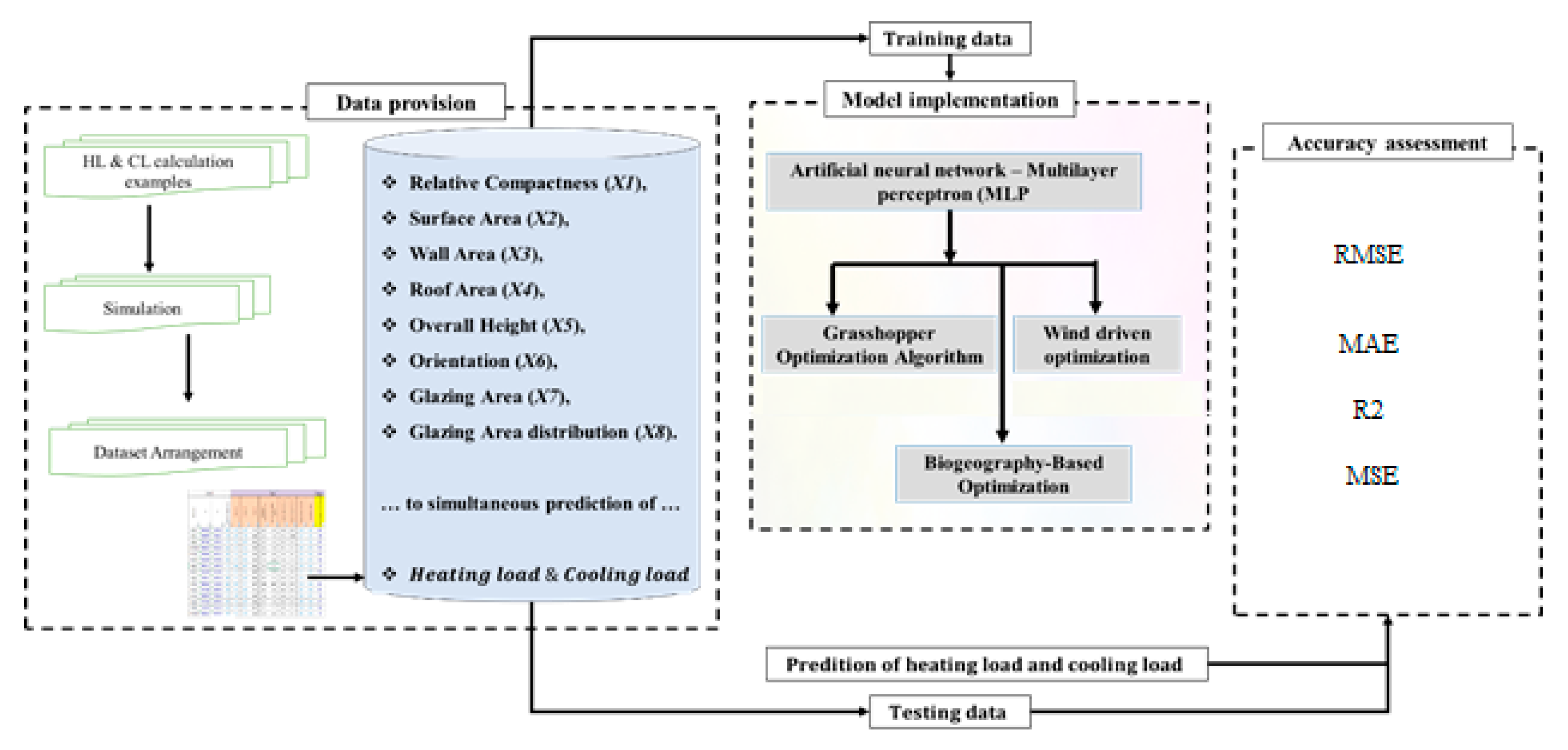
The steps that are taken to fulfill the objective of the current study are illustrated here as well as in Figure 1:
- (a)
- First, data preprocessing: in this step, the collected dataset of heating loads and cooling loads are separated randomly into two main sections called the training dataset and testing dataset. As a well-established train/test dataset selection, 70% of the whole dataset is used for training the models to create a proper predictive network and to make the connection between both targets of HLs and CLs and their influential factors. The rest of the 30% is selected to be the testing and validation datasets. In our example, we selected 30% for the testing dataset, where none of the testing datasets were involved in the learning process.
- (b)
- Second, the programming language of MATLAB 2018 is used to (i) define the most proper structure of the multi-layer perceptron (MLP) neural network (in terms of the number of hidden neurons), and (ii) building three hybrid models by optimizing the computational parameters of the MLP (that is, its biases and assigned weights) using the GOA, WDO, and BBO algorithms. After a series of trial and error parametric processes (that is, used to find the most appropriate hyperparameters of the hybrid models), the best population size is determined for each model. Next, the outputs (that is, HLs and CLs in our study) are predicted by the proposed models.
- (c)
- In the last step, by employing the remaining 30% of data (that is, called the testing dataset), the error performance of the proposed models is calculated based on the differences between the real measured values and the predicted values obtained from the proposed models.
The following, sections describe the MLP, GOA, WDO, and BBO algorithms that were used.
2.1. Multilayer Perceptron
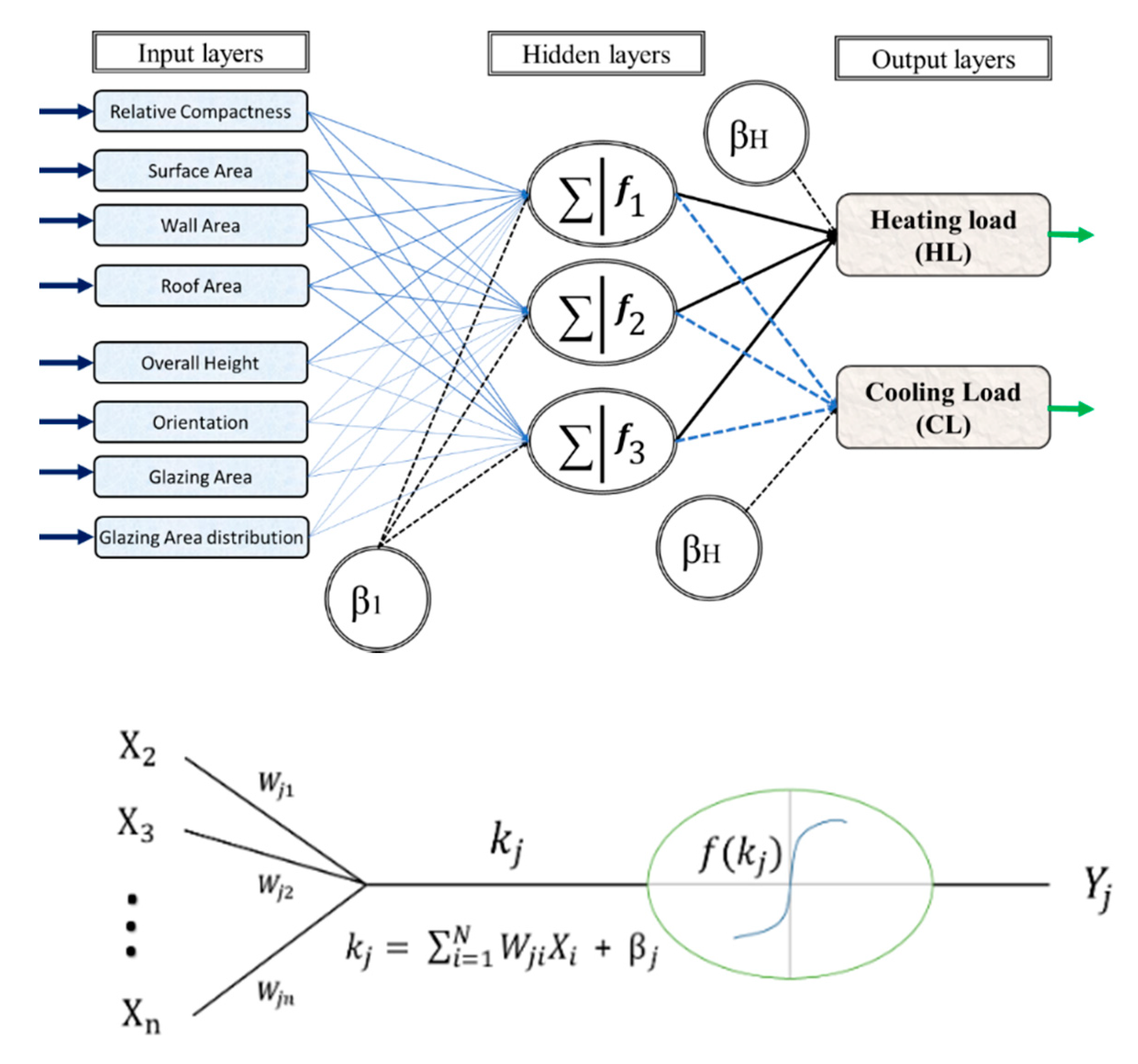
These tools are widely applied for modeling complex engineering issues. Artificial neural networks (ANNs), (that is, also called neural networks) were first introduced by McCulloch and Pitts [114]. It is known as a computing system vaguely inspired by the biological neural networks, whose idea is primary taken from animal brains. This artificial intelligence (AI)-based technique will try to make a relationship between a series of input data layers with one or more output layers by establishing non-linear equations [115]. A common ANN structure includes different elements called input layers, hidden layer(s), and output layer(s) (Figure 2).
2.2. Grasshopper Optimization Algorithm
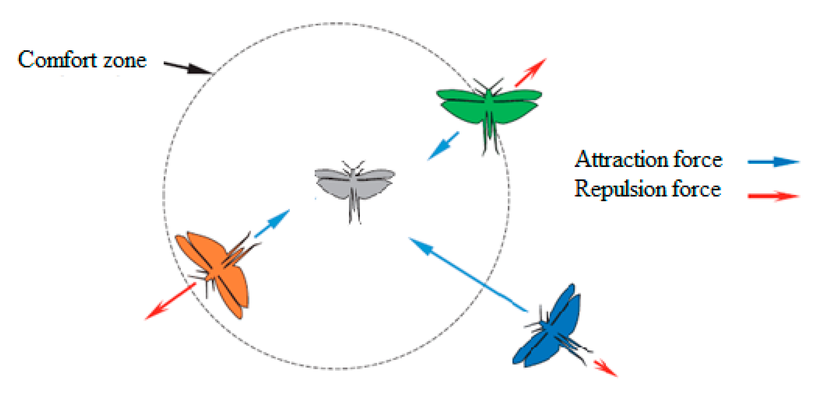
Grasshoppers may be seen independently or in a swarm in nature. It is considered as one of the insects feeding on plants. Noting that such insects are considered as a pest (that is, any plant or animal detrimental to crops) as they mainly severely harm the crops and pasture [116]. The idea of the grasshopper optimization algorithm (GOA) is taken from the natural behaviors of grasshoppers pests; Saremi, et al. [117] developed the GOA for solving searching optimization issues. Like many previously published natural inspired algorithms (for example, the whale optimization algorithm; the ant lion optimizer; the salp swarm algorithm, etc.), the GOA algorithm predicts based on two major steps. The first step is an exploration whereas the second step is called exploitation. As is taken from the grasshoppers’ behaviors, such steps are performed to seek a food source. In this first phase (that is, called the exploitation phase), the agents that are responsible for the search fly locally over the search area. This process is illustrated in Figure 3. which is adapted from [117]. According to Mafarja, et al. [118], which explored the behavior of the relations for different levels of some algorithm parameters, when the distance between two grasshoppers is between 0 and 2.079, the repulsion takes place between them. Consequently, if the distance is out of this range (that is, larger than 2.079), it means that the proposed grasshopper enters a comforting district.
Equation (1) expresses the movement of grasshoppers, noting that the term xi is the position of the ith insect:
where r1, r2, and r3 are random values between 0 and 1. Also, Si, Gi, and Ai denote the social relationship, the gravity force, and the wind advection, respectively.
2.3. Wind-Driven Optimization
The technique of wind-driven optimization (WDO) was introduced by Bayraktar, et al. [119]. The early idea of WDO was initially formed for electromagnetics usages. In this sense, the four most influential forces for this task are a Coriolis force (FC), pressure gradient force (FPG), frictional force (FF), and gravitational force (FG). The main idea behind the WDO method is that, for reducing the computational complexity, the air parcels are considered weightless and dimensionless. Assuming that δV and the ∇P are the finite volume and pressure gradient of the air, and Equation (6) shows the main force because of the pre-defined pressure gradient. The FF (as it is shown by Equation (7)) aims to face the air-triggered movement by the term FPG. In this regard, the term FG (that is, the gravitational force illustrated by Equation (8)) pulls the parcels to the earth’s center from every dimension. Also, the FC (Equation (9)) attributes to the deflection in the air parcel motions.
In Equations (6)–(8), the term is set to be the velocity vector of wind, is the density of a short air parcel, g signifies the gravitational constant, symbolizes the earth’s rotation and finally is a frictional coefficient.
By considering the above-mentioned influential factors and pre-defined forces along with the ideal gas equation, the finalized equation is provided by Derick, et al. [120]:
Since the air velocity mainly depends on the pressure value the velocity gets adjusted to bring higher pressure for the system.
Therefore, regarding the pressure rank, Equation (10) is adapted. In this sense, due to the pressure, the known parcels, in a descending sequence, are ranked. Accordingly, the position and velocity are updated by the following equations when i denotes the rank:
where in Equations (7) and (8), the terms and signify the velocity value of the current and coming iteration, respectively. Note that the term x is defined to be the air parcel position. In addition, and are set to be the optimal and current positions, respectively. Meanwhile, the other terms such as are set to be equal while the C is taken to calculated as C = −2 . The clarified progressive process updates until stopping criteria are met. These criteria can be set by an objective function or even a pre-defined number of repetitions. Full details of the WDO technique is explained in some previous studies such as Bayraktar, et al. [119] and Bayraktar, et al. [121].
2.4. Biogeography-Based Optimization
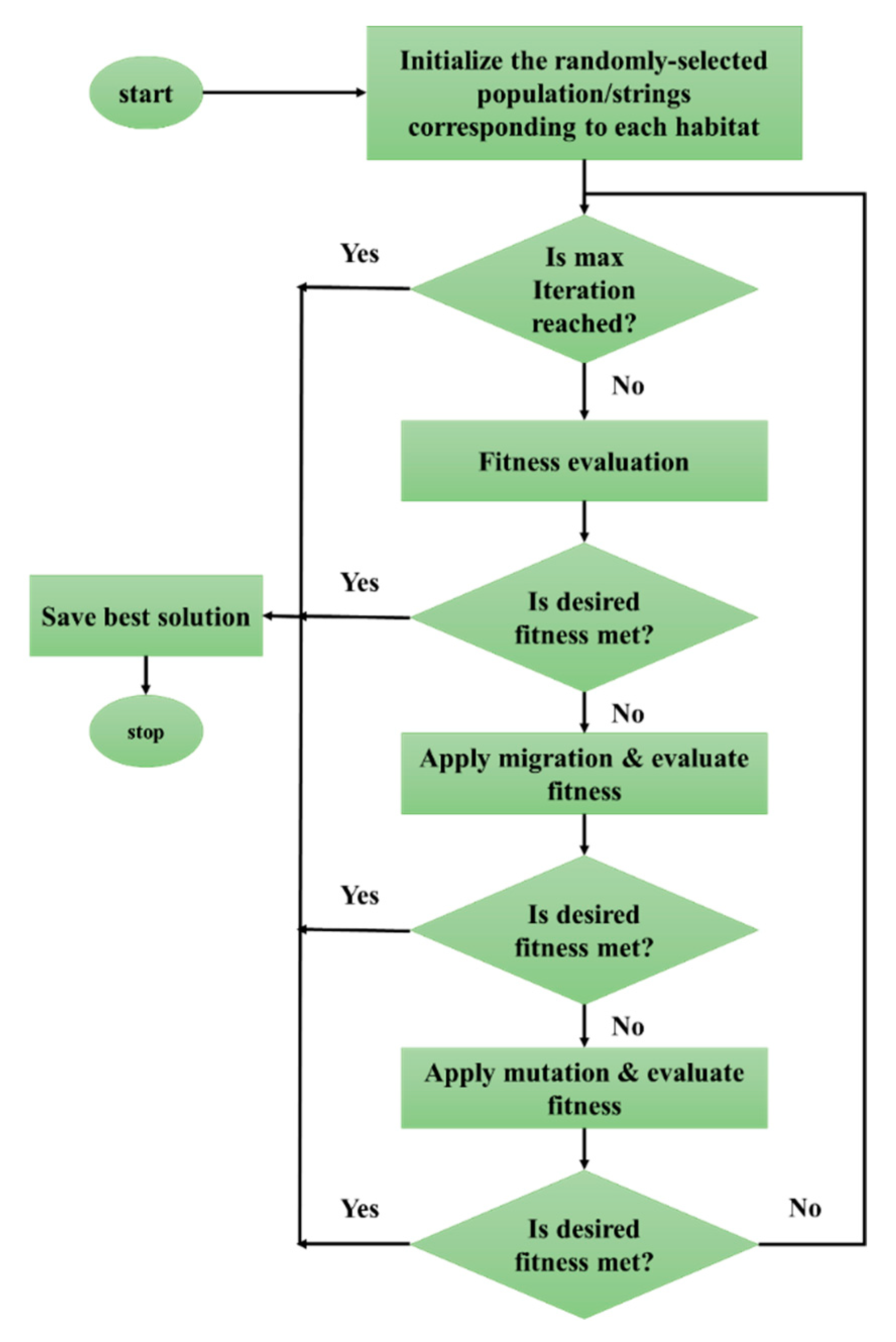
BBO was established based on the nature of different species distribution as well as their biogeography knowledge. BBO was first developed by Simon [54]. Later it was expanded by other researchers and more particularly by Mirjalili et al. [55], where the initial algorithm was enhanced and combined with MLP structure and became BBO-MLP. Due to its excellent predictivity, many scholars recommended it to be used in many complex engineering problems [122,123]. A combination with MLP aimed to optimize the performance of the MLP since the BBO is known as a population search based technique. The flowchart of the original algorithm before being mixed with MLP is shown in Figure 4. Which is adopted from [54,55]. Similar to many other population search-based optimization algorithms, the BBO also gets started by generating a random population called a habitat.
3. Data Collection and Statistical Analysis
The primary dataset of this study is obtained from Tsanas and Xifara [124] as uploaded in an open-source machine learning repository (http://archive.ics.uci.edu/ml/datasets/Energy + efficiency accessed on 26 December 2020). The dataset was prepared according to the Ecotect computer software [125], where 12 different types of residential buildings (hypothetically located in Athens, Greece, each containing 7 persons with the area of 771.75 m3 composed of 18 elementary cubes with dimensions of 3.5 × 3.5 × 3.5 m3) with changes in their influential design parameters simulated. Common material with U-values of 1.780, 0.860, 0.500, and 2.260 for walls, floors, roofs, and windows, respectively, was used for simulating the buildings. Calculating the glazing areas as a ratio the floor area, three areas with the ratios 10%, 25%, and 40% are considered. Applied distributions of this parameter are as follows:
- (a)
- uniform: with 25% glazing on each,
- (b)
- north: 55% on the north and 15% on each other side,
- (c)
- east: 55% on the east and 15% on each other side,
- (d)
- south: 55% on the south and 15% on each other side, and
- (e)
- west: 55% on the west and 15% on each other side.
Some samples also did not have glazing areas.
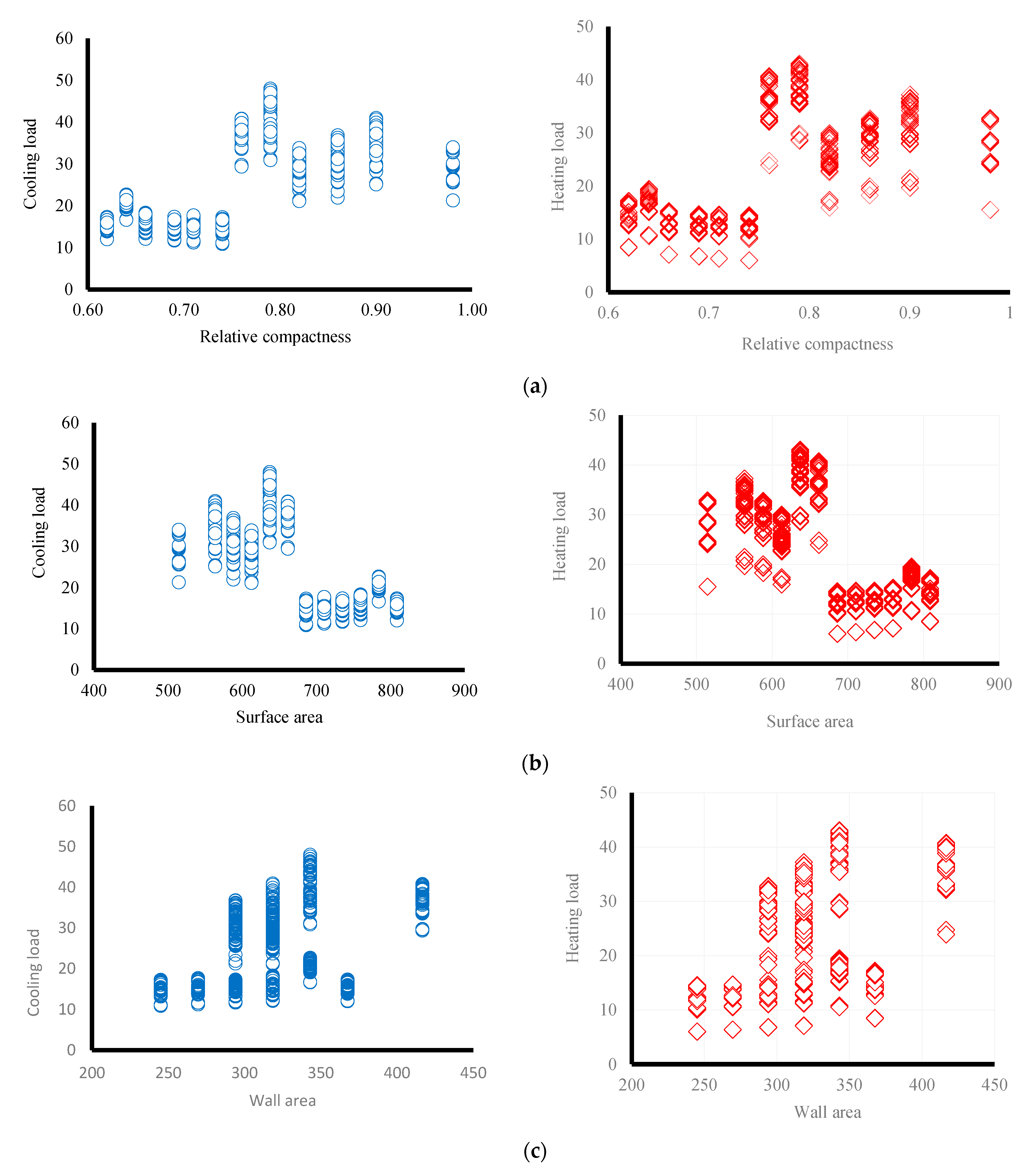
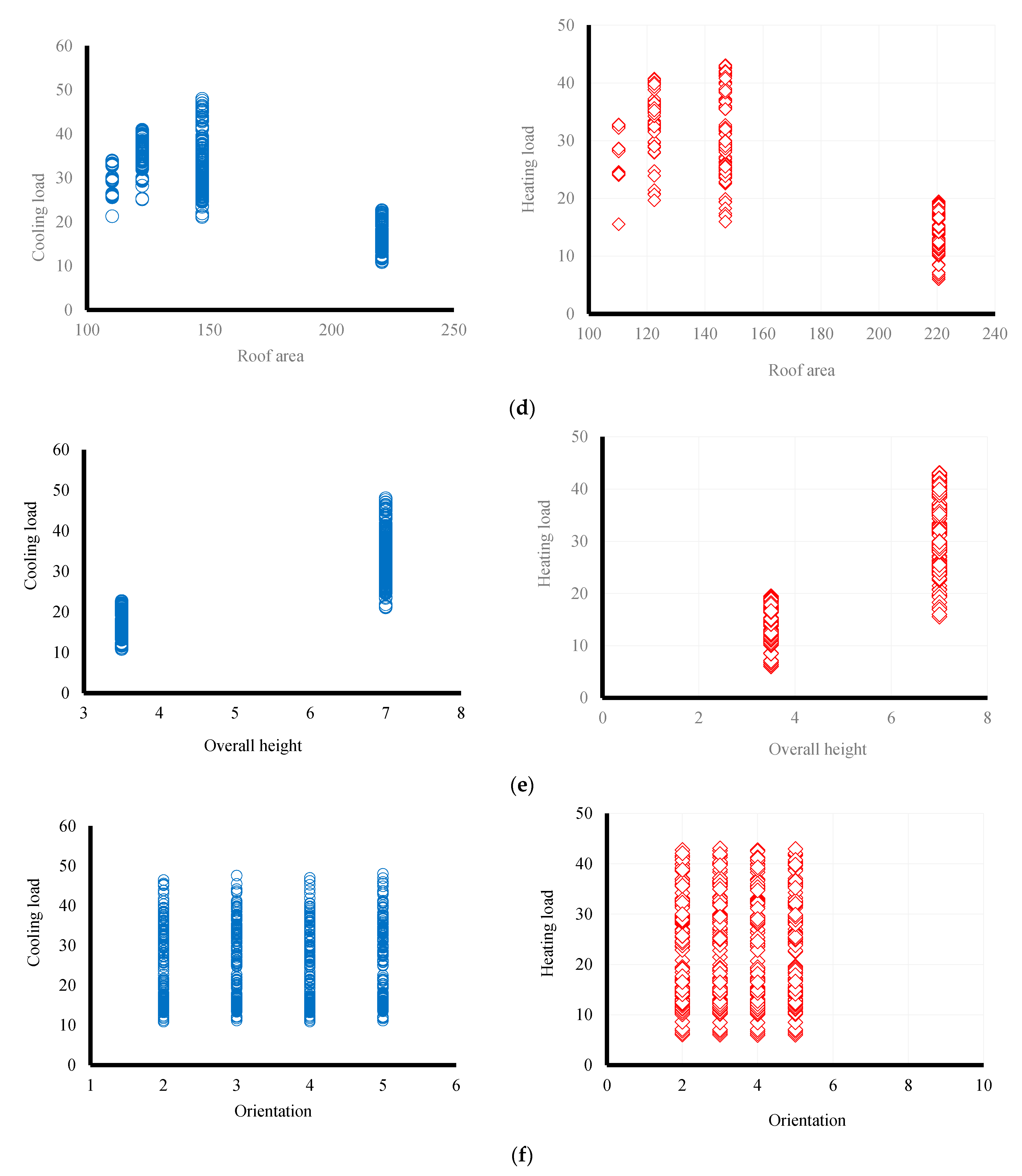
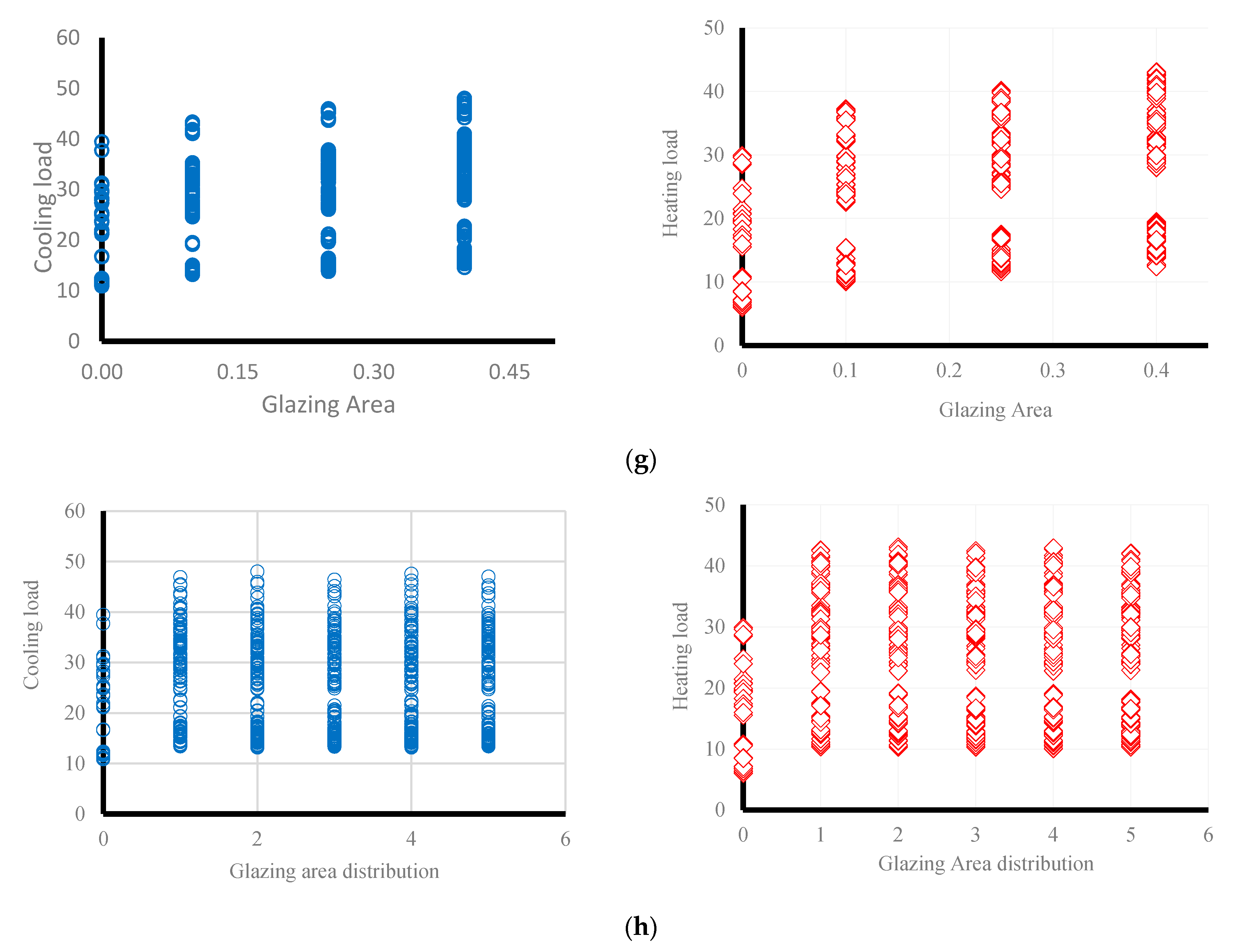
The main objective was to measure the values of HL and CL (both in kWh/m2) based on the designated residential buildings. Each one of the proposed residential buildings follows a unique structure, such as variation in their design parameters such as relative compactness, roof area, surface area, wall area, orientation, glazing area distribution, overall height, and glazing area. For instance, four orientations, five distribution scenarios, four sets of glazing areas (such as 0, 10, 25, and 40% of the entire floor area), etc. Therefore, a total of 768 design examples were simulated accounting for eight key design factors. The targets were both HL and CL that were required for the particular residential buildings. More description of the employed dataset can be obtained in other related studies such as Chou and Bui [126] and Tsanas and Xifara [124]. In this article, both of the HL, as well as CL, are taken into the calculation procedure as the main target variables. The main aim was that these targets to be predicted by the three proposed hybrid intelligence techniques including GOA-MLP, WDO-MLP, and BBO-MLP. The main dataset includes 768 samples, 537 rows (i.e., 70%) are chosen for designing the training pattern, and the rest of the 231 rows (that is, 30%) are taken to assess the validation and to test the trained networks. The scatter plots of Figure 5 show the influential factors that have been used as the main inputs and their relationship with both chosen targets of HL and CL. To help to understand the variability of the provided datasets, the descriptive statistics of the input variables are provided and tabulated in Table 1.
4. Results and Discussion
This investigation aimed to predict HLs and CLs in buildings utilizing artificial intelligence according to predictive tools. An ANN multilayer perceptron (MLP) is employed to estimate the HLs and CLs. The prepared datasets are separated into two sections, for training and testing the model. The first section that is selected using 70% of the whole database is considered for training of the ANN models (named training dataset) while the 30% remaining items are used for evaluation of their network performances (called the testing dataset). The new testing dataset (that is, selected in each stage of the network simulation) is built using data that varies from the training step. Two statistical indices of the determination coefficient (R2) and root mean square error (RMSE) are employed to compute the network error efficiency and the regression among the target values and system outcomes of HLs and CLs. The upper mentioned indices are significantly utilized and also are presented by Equations (9) and (10), respectively.
where, Yi actual, Yi produced, and Ymean indicate values considered in each step of the simulation for the exact, predicted, and the mean values of the shown Pult, respectively. N displays the number of data.
4.1. Optimization of MLP Model
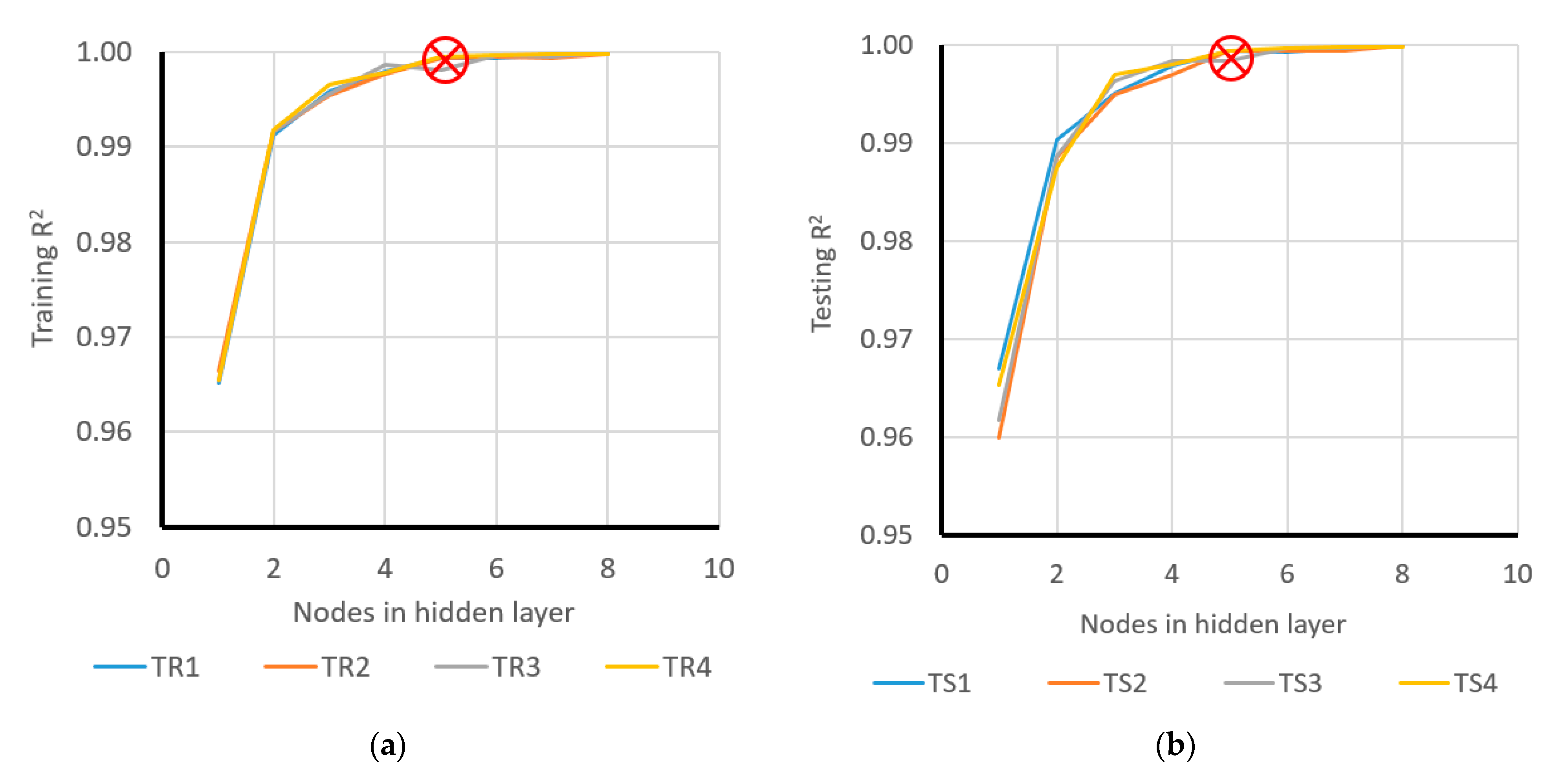
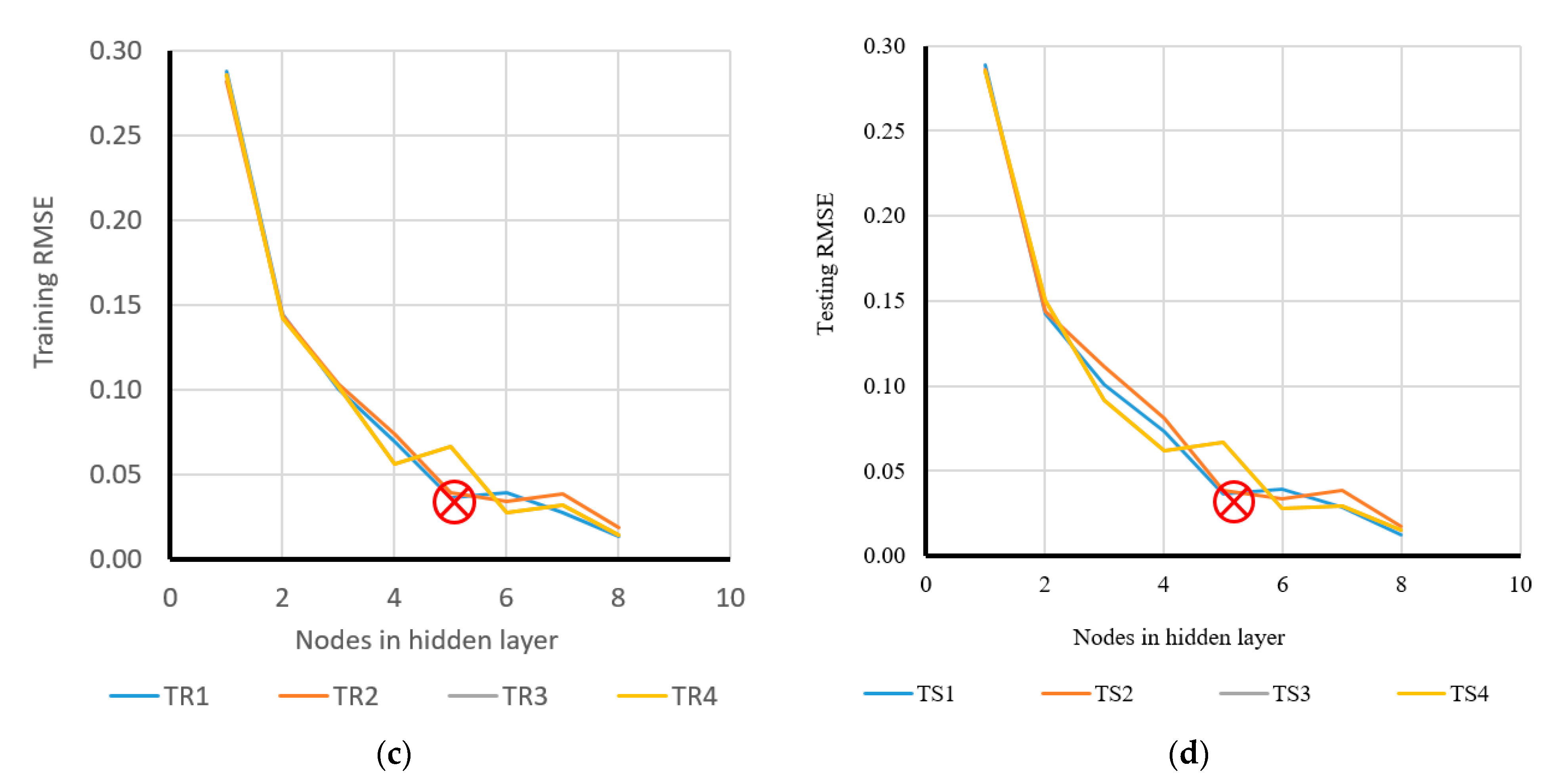
Before training the models using GOA, WDO, and BBO, a reliable primary structure of the MLP should be determined. In a multilayer perceptron-based network model, the number of neurons for the output and input layers is fixed. Such a number is considered to be equal to the number of outputs and inputs, respectively. It is important to know that this number in the hidden layer is a different factor that changes relying on the amount of user data. So, in this step and to create a strong multilayer perceptron-based network structure, eight different numbers were tested for the hidden neurons. For more trustworthiness, each of the proposed networks was implemented four times (shown as TR1, TR2, TR3, and TR4 indicating the first, second, third, and fourth effort, respectively), and totally, thirty-two (= 4 ∗ 8) various structures were built to specify the most proper structure. Figure 6 shows the results of the considered analysis. This trial and error procedure can help to determine the best structure of the optimized network. The best structure of the MLP model, having the minimum error, may be achieved while the number of neurons in each hidden layer is 5. Accordingly, to have a simplified solution and as shown in Figure 6, the number of nodes equal to five was selected as the best possible number of neurons that are required to be chosen in the hidden layers. SO, the network structure is obtained to be 8 × 5 × 2 (that is, eight input neurons, five hidden neurons, and two output neurons).
The mathematical-based equation of the obtained MLP structure was given (as a problem function) to the GOA, WDO, and BBO optimization algorithms to be trained. This process consists of finding the best set of weights and biases for a raw MLP structure. The prediction is then executed by the optimized MLP.
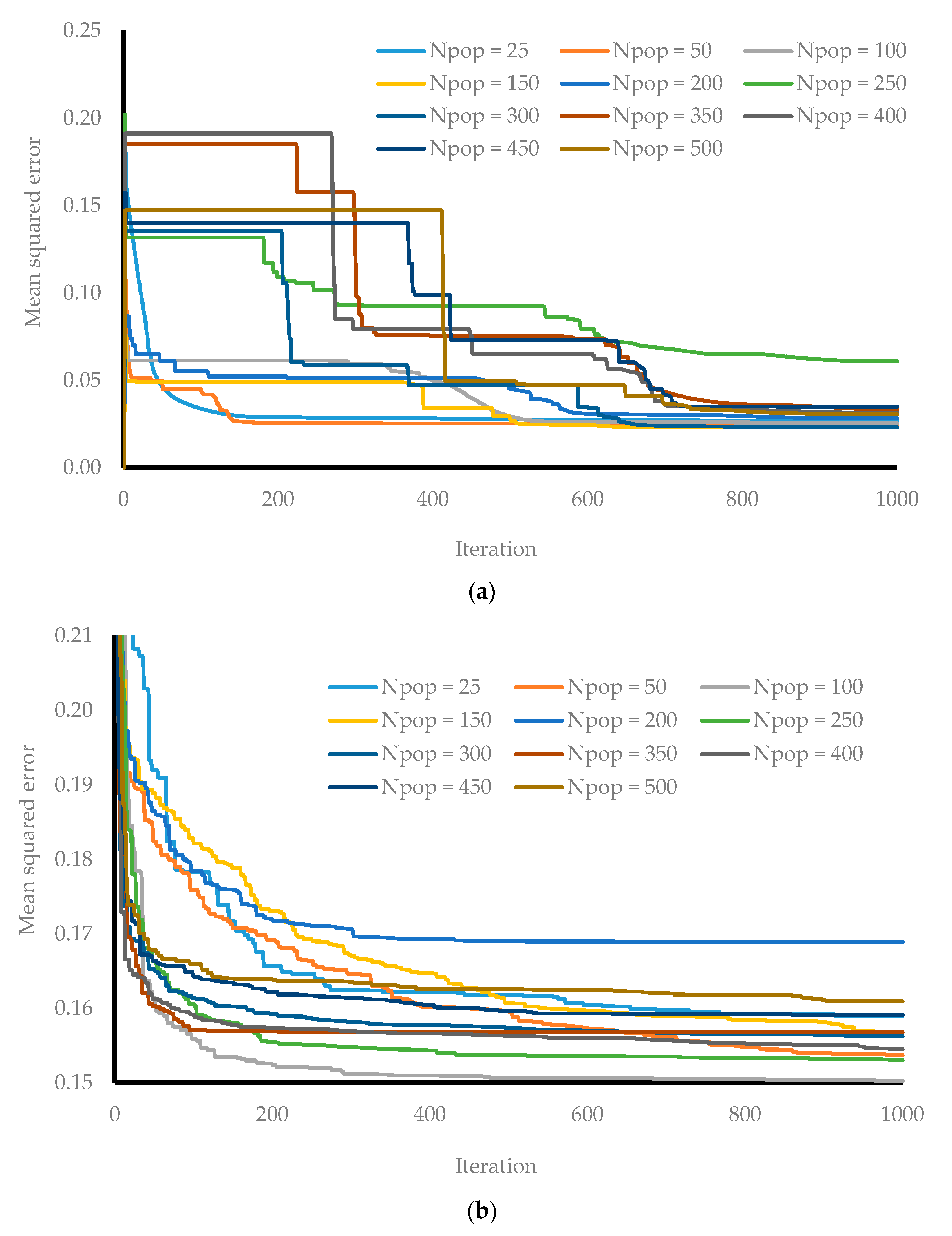
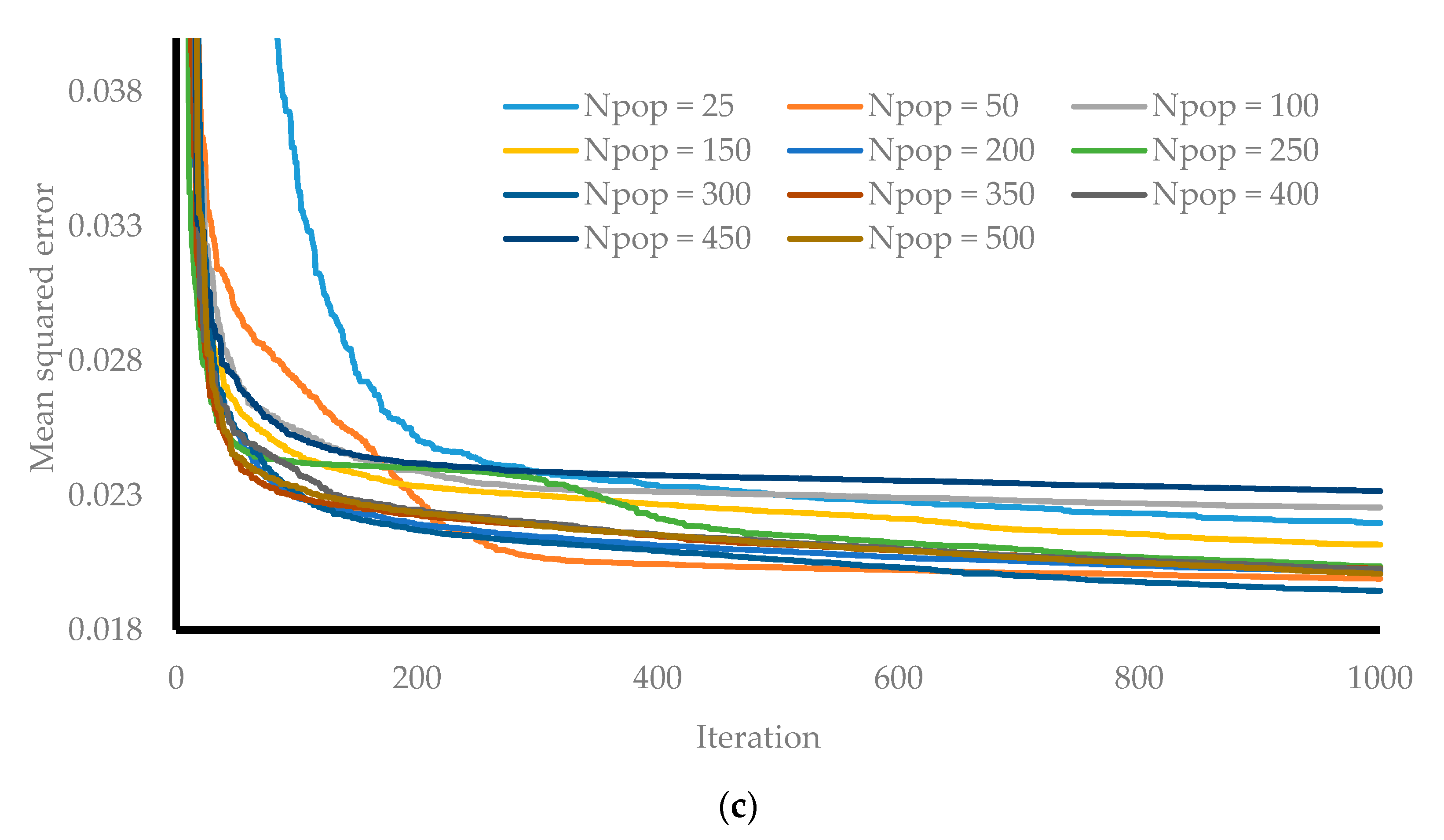
The next step deals with selecting the proper cost function, object function, and assessment techniques (for example, R2 and RMSE). In this step, we try to provide the best-fit relationships between the actual and predicted values. In the current study, two simultaneous target simulations were provided for both HLs and CLs. As described, at the end of each iteration the value of the cost function is taken to assess the accuracy of the proposed model. In this sense, a sensitivity analysis was then performed for all proposed models of GOA-MLP and WDO-MLP based on the population size (also known as the swarm size). It is one of the most critical terms for hybrid intelligent algorithms. Therefore, the hybrid predictive networks are assessed according to various swarm sizes (for example, in this study, nine sets of swarm sizes were used), leading to 11,000 iterations for every one of the proposed hybrid solutions. The swarm size varied between 25 to 500 as shown in Figure 7. All the algorithms conducted 1000 iterations to find enough chances to decrease the rate of errors shown here as mean square errors. The convergence curves that are shown in Figure 7 are the first result of the fitness function after the swarm size sensitivity analysis. This part is also called the convergence analysis. As depicted in Figure 7a–c, respectively, for the GOA-MLP, WDO-MLP, and BBO-MLP ensembles, the higher iterations normally caused a decrease in the rate of MSE errors. Nonlinear swarm-based analysis for the estimation of the GOA-MLP, WDO-MLP, and BBO-MLP of the heating load in energy-efficient buildings are tabulated in Table 2, Table 3 and Table 4, respectively.
4.2. Assessment of the Proposed Models
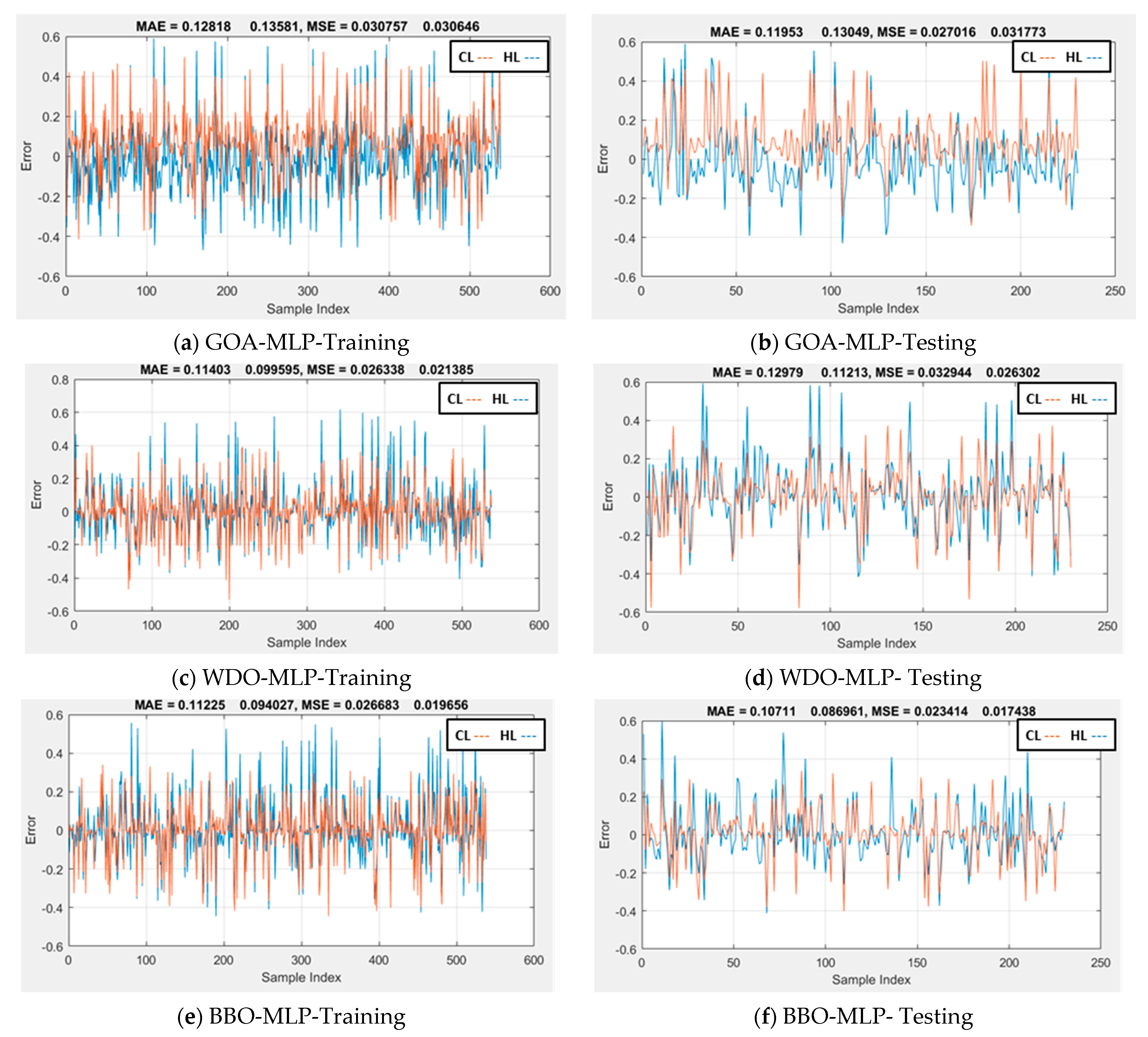
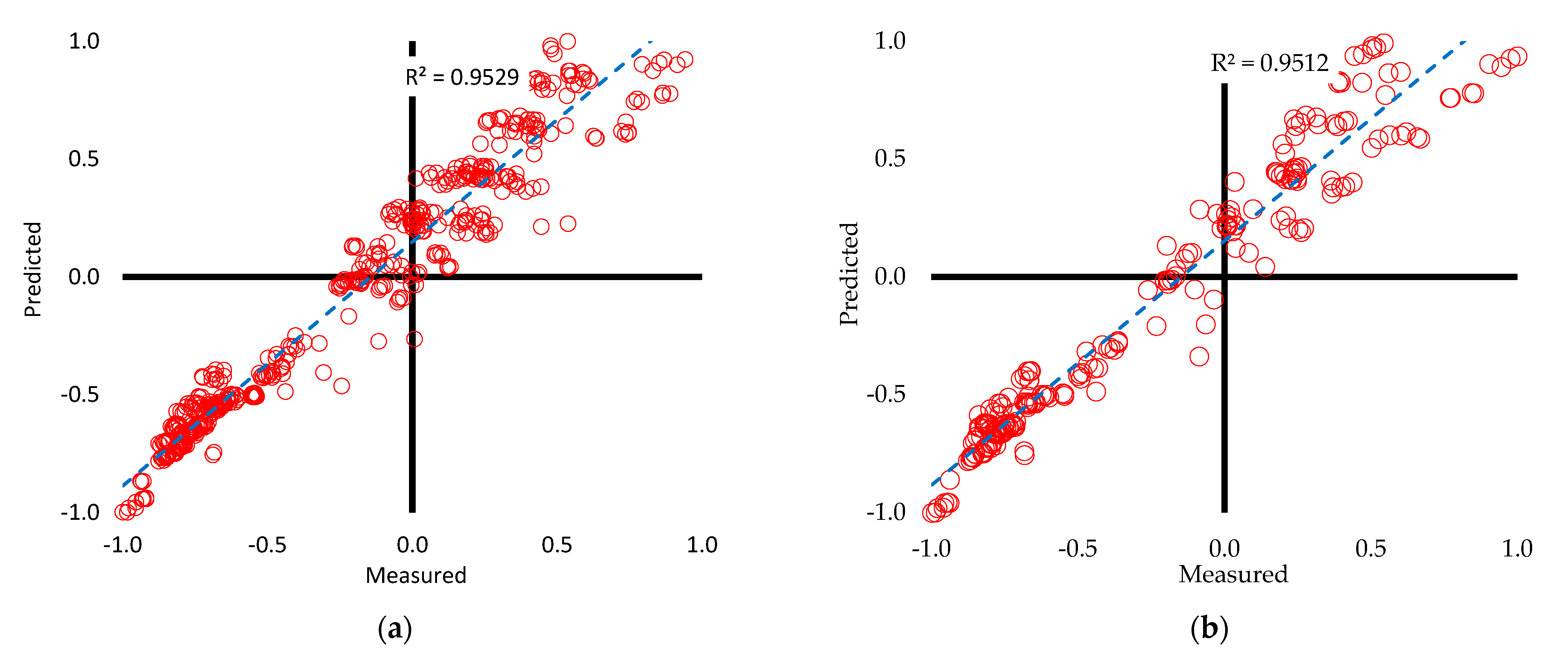
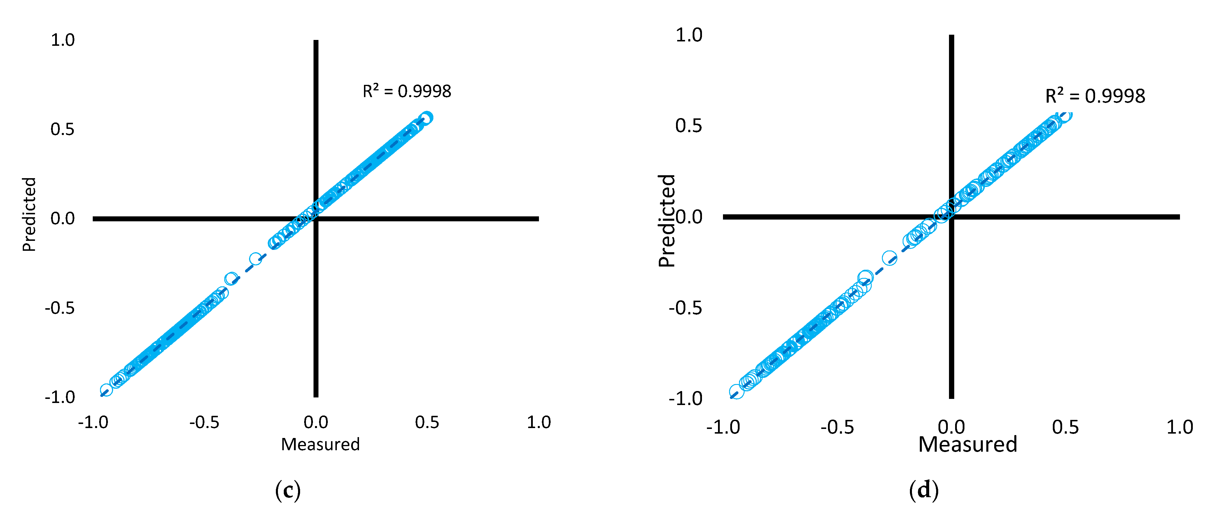
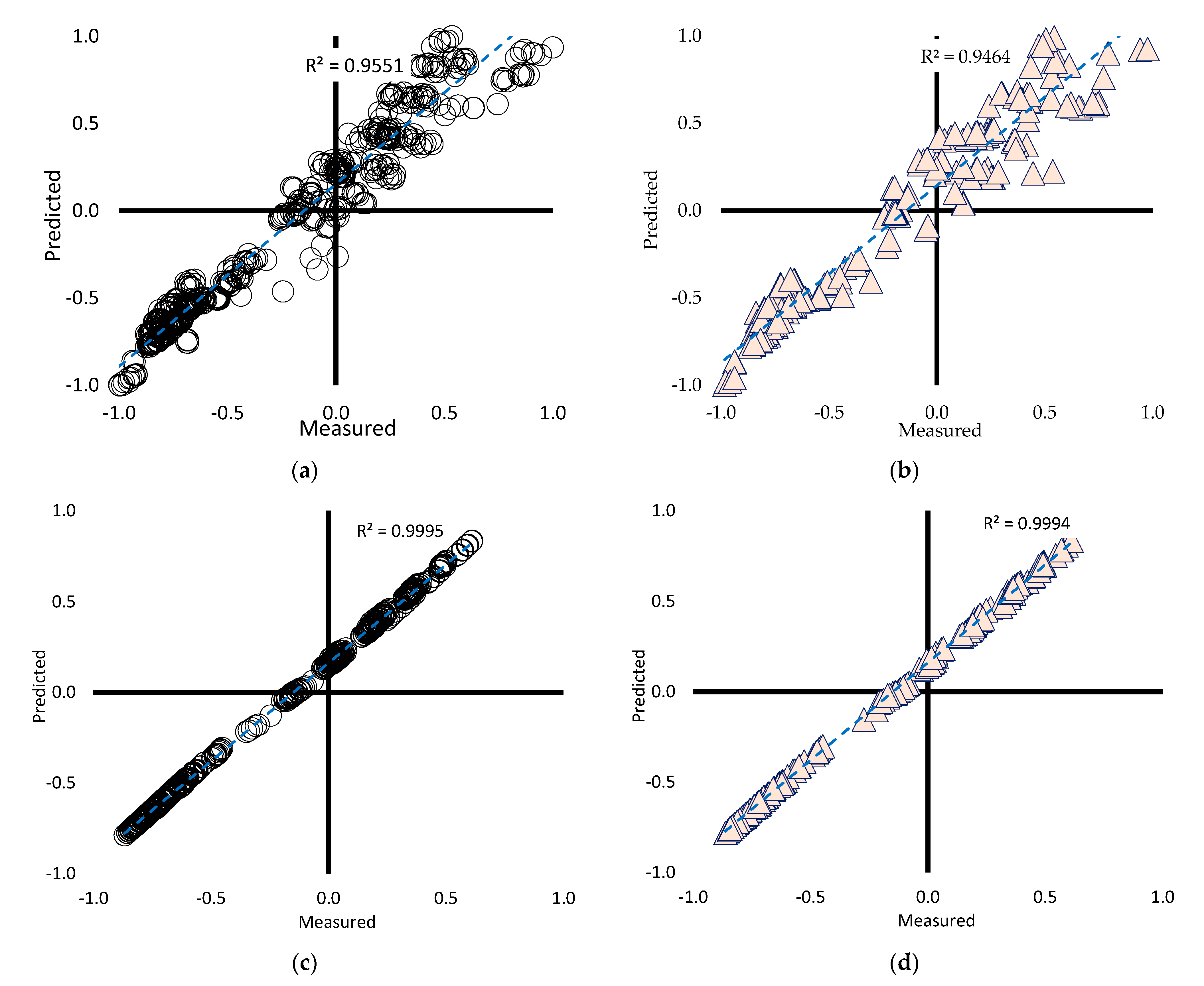
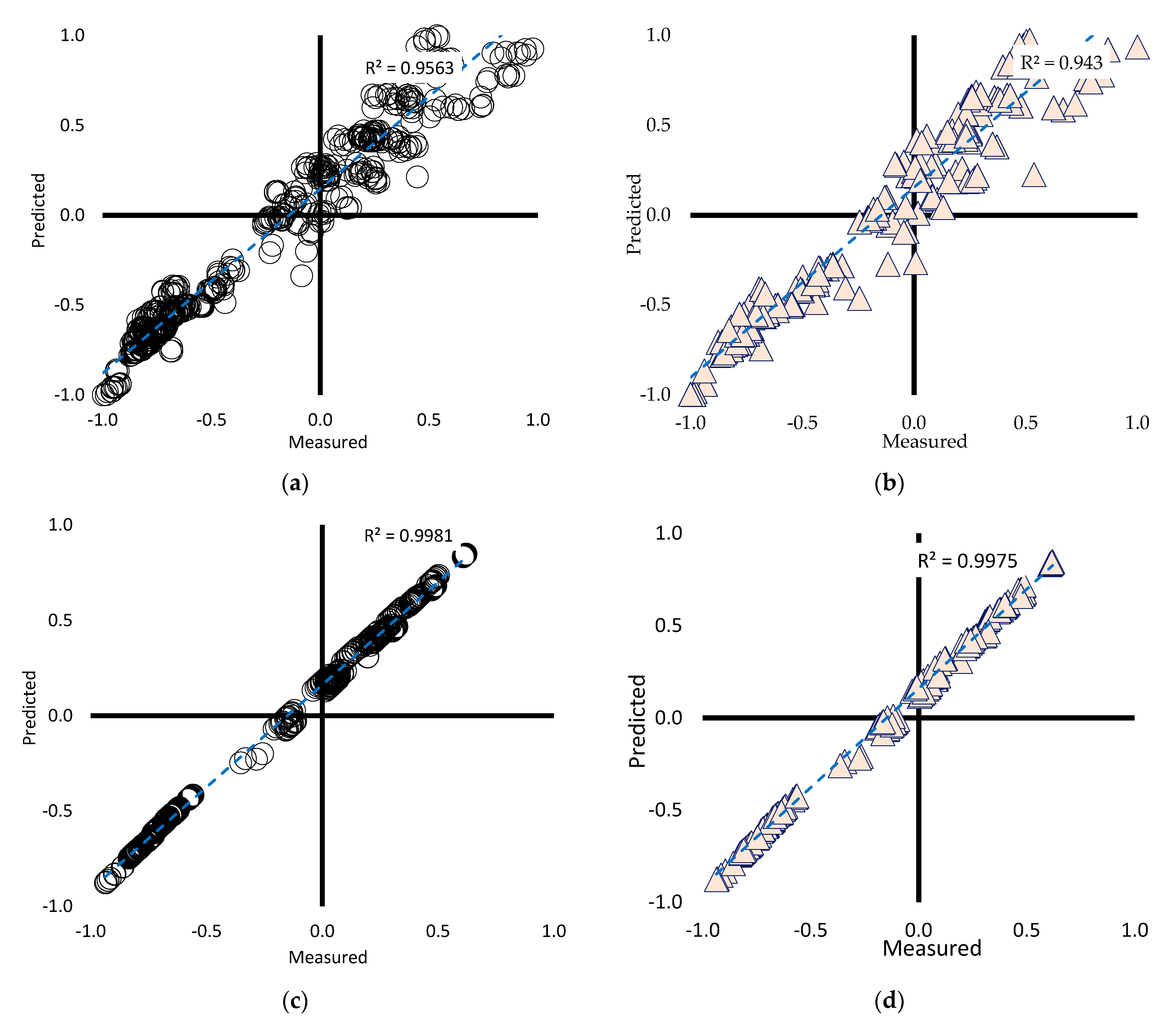
The reliability of the proposed models is assessed by evaluating the measured and predicted values of the HLs and the CLs. Two different sets of error criteria of MSE and RMSE are used to have an estimation of the error as well as checking the performance of samples obtained from both training and testing datasets. It is worth noting that the output fitness from both of the training and testing phases defines the generalization power and training capability, respectively. The computed error values in the simultaneous HL and CL prediction for GOA-MLP, WDO-MLP, and BBO-MLP techniques are also shown in Figure 8. Figure 9 (referred to as GOA-MLP) and Figure 10 (referred to as WDO-MLP) display a graphical evaluation between the original predicted and measured patterns of the heating and cooling loads (for both the training and testing datasets). Similarly, the accuracy of the proposed multitarget prediction BBO-MLP techniques are shown in Figure 11. As is seen, all proposed models result in a valid estimate of the HLs and CLs patterns: with the calculated R2 (training = 0.9529, testing = 0.9512) for the GOA-MLP-HLs and R2 of (training = 0.9998, testing = 0.9998) for the CLs estimation. In the case of WDO-MLP-HLs, the R2 (training = 0.9551 and testing = 0.9464) was calculated while for the WDO-MLP-CLs, the R2 (training = 0.9995 and testing = 0.9994) was found. Lastly, for the case of BBO-MLP-HLs, the R2 (training = 0.9563 and testing = 0.943) and BBO-MLP-CLs, the R2 (training = 0.9981 and testing = 0.9975) were calculated. Considering the three proposed techniques and after performing a nonlinear swarm optimization process, it can be seen that the best-fit model is obtained from the proposed structure of BBO-MLP. The result from the error evaluations also shows excellent accuracy, and this proved the BBO-MLP is the most effective hybrid technique in training the MLP.
4.3. Simplified Multitarget Equation
To have a more practical formula that can be used to predict both HLs and CLs and considering the minimum required error, in this section, a simple MLP network (having two neurons in its hidden layer) is provided. Also, to have a better understanding, the MLP-best-fit equation is prepared according to the optimized weights and biases. These terms are unique for any particular database. Noting that to have practical use of this formula, the well-known mathematical function of Tangent-Sigmoid (Tansig) is also provided. The Tansig is also the MLP activation function expressed by Equation (14). The R2 accuracy of the proposed formula for the prediction of multi targets of HLs and CLs simultaneously were 0.98547, 0.9866, 0.98374 for the training, testing, and validation datasets, respectively.
where
in which A, B, C, D, E, F, G, and H represent relative compactness, surface area, wall area, roof area, overall height, orientation, glazing area, and glazing area distribution, respectively.
HL = 2.5988 × Y1 − 2.7980 × Y2 − 1.1800
CL = 2.2978 × Y1 − 2.5449 × Y2 − 1.1861
CL = 2.2978 × Y1 − 2.5449 × Y2 − 1.1861
Y1 = Tansig(5.7372 × A + 2.0859 × B + 3.1483 × C + 2.1314 × D − 1.7433 × E − 0.0017 × F + 0.0034 × G − 0.0051 × H + 2.8682)
Y2 = Tansig(−0.6890 × A − 0.3583 × B − 0.1591 × C − 1.8659 × D − 1.8637 × E − 0.0034 × F − 0.1021 × G − 0.0128 × H + 0.6117)
4.4. Further Discussion and Future Works
The high significance of predicting the thermal load of buildings has driven many scholars toward developing sophisticated methods for predicting the heating load and cooling load. This subject is particularly important when it comes to energy-efficient buildings [127]. The findings of this study are in accordance with earlier efforts regarding the applicability of artificial intelligence models for simulating the HL and CL. These studies have focused on various types of buildings including office, residential, and industrial buildings [128,129].
Data-driven methods (for example, MLP ANN) are capable of analyzing the relationship between a number of effective parameters with a target parameter that is aimed to be predicted. The HL and CL of a residential building were successfully modeled in this study using three hybrid techniques. Each model represented an MLP neural network optimized with a metaheuristic algorithm. The optimizer components were the grasshopper optimization algorithm, wind-driven optimization, and biogeography-based optimization. These algorithms can globally find the solution to a given problem. In this work, evaluating different population sizes for the mentioned hybrids (Figure 7) showed that although the results of similar population sizes are somewhat close the effect of this parameter is better investigated to use an appropriate configuration.
Having a look at the dataset that was used (Figure 5), most of the inputs (for example, glazing area distribution) do not show an explicit correlation with the target parameters; this indicates the complexity of the problem. In such cases, a powerful algorithm can prevent the network to be misled. As the results showed, the GOA, WDO, and BBO could nicely deal with this problem; meaning that they could predict the loads for buildings with both high and low inputs.
Due to the excellent performance of all algorithms that were used, determining the best-fitted model can be disputable, but overall, considering both correlation and error evaluations for both targets, the BBO-based model was slightly better. It indicates that the MLP parameters optimized by the bio-geography theory are more efficient compared to those found by the grasshopper optimization algorithm and wind-driven optimization.
The formula provided at the end of this research is reliable due to the excellent correlation of its products. However, considering the dataset that was used, it may be subjected to residential buildings. As explained supra, the data of this study was obtained from a computer simulation for various types of residential buildings. An idea for future work can be utilizing the type of buildings as an input to archive a more generalizable solution.
5. Conclusions
This article is concerned with the simultaneous calculation of HLs and CLs of residential buildings through the HVAC system. To limit the drawbacks of MLP technique, hybrid intelligent techniques are implemented. The focus of the three proposed models abbreviated as GOA-MLP, WDO-MLP, and BBO-MLP was to introduce several reliable novel hybrid models to simulate both HLs and CLs. Overall, and after 33,000 iterations of the three proposed algorithms, it was shown that all three hybrid techniques (GOA-MLP, WDO-MLP, and BBO-MLP) can nicely deal with the prediction task. However, the accuracy of the BBO-based model was slightly higher. Moreover, assessing the results revealed that the CLs results are associated with higher accuracy. Since the CLs prediction was almost equal to the real values, the main comparison was made based on the values of predicted HLs. Although the findings of this paper led to three novel sophisticated approaches for the indirect modeling of building thermal load, the comprehensiveness of the proposed models can be improved by using the data of other types of buildings as well.
Author Contributions
Conceptualization, H.M. and A.M.; methodology, H.M. and A.M.; software, H.M. and A.M.; validation, H.M. and A.M.; formal analysis, H.M. and A.M.; investigation, H.M. and A.M.; resources, H.M. and A.M.; data curation, H.M. and A.M.; writing—original draft preparation, H.M. and A.M.; writing—review and editing, H.M. and A.M.; visualization, H.M. and A.M.; supervision, H.M. and A.M.; project administration, H.M. and A.M.; funding acquisition, H.M. and A.M. All authors have read and agreed to the published version of the manuscript.
Funding
This research received no external funding.
Institutional Review Board Statement
Not applicable.
Informed Consent Statement
Not applicable.
Data Availability Statement
Not applicable.
Acknowledgments
This research is in part supported by the Alexander von Humboldt Foundation and the open access funding by the publication fund of the TU Dresden.
Conflicts of Interest
The authors declare no conflict of interest.
References
- US EIA. Total Energy. Annual Energy Review. U.S. Department of Energy (DOE). Available online: https://www.eia.gov/totalenergy/data/annual/index.php (accessed on 10 November 2017).
- IEA, International Energy Agency. Key World Energy Statistics; IEA: Paris, France, 2015. [Google Scholar]
- Zhou, Y.K.; Zheng, S.Q.; Zhang, G.Q. Artificial neural network based multivariable optimization of a hybrid system integrated with phase change materials, active cooling and hybrid ventilations. Energy Conv. Manag. 2019, 197, 19. [Google Scholar] [CrossRef]
- Ahmad, A.S.; Hassan, M.Y.; Abdullah, M.P.; Rahman, H.A.; Hussin, F.; Abdullah, H.; Saidur, R. A review on applications of ANN and SVM for building electrical energy consumption forecasting. Renew. Sustain. Energ. Rev. 2014, 33, 102–109. [Google Scholar] [CrossRef]
- Mocanu, E.; Nguyen, P.H.; Gibescu, M.; Kling, W.L. Deep learning for estimating building energy consumption. Sustain. Energy Grids Netw. 2016, 6, 91–99. [Google Scholar] [CrossRef]
- Wang, Z.; Hong, T.; Piette, M.A. Building thermal load prediction through shallow machine learning and deep learning. Appl. Energy 2020, 263, 114683. [Google Scholar] [CrossRef] [Green Version]
- Hu, L.; Hong, G.; Ma, J.; Wang, X.; Chen, H. An efficient machine learning approach for diagnosis of paraquat-poisoned patients. Comput. Biol. Med. 2015, 59, 116–124. [Google Scholar] [CrossRef] [PubMed]
- Wang, S.-J.; Chen, H.-L.; Yan, W.-J.; Chen, Y.-H.; Fu, X. Face recognition and micro-expression recognition based on discriminant tensor subspace analysis plus extreme learning machine. Neural Process. Lett. 2014, 39, 25–43. [Google Scholar] [CrossRef]
- Chao, M.; Kai, C.; Zhiwei, Z. Research on tobacco foreign body detection device based on machine vision. Trans. Inst. Meas. Control 2020, 42, 2857–2871. [Google Scholar] [CrossRef]
- Wang, M.; Chen, H.; Yang, B.; Zhao, X.; Hu, L.; Cai, Z.; Huang, H.; Tong, C. Toward an optimal kernel extreme learning machine using a chaotic moth-flame optimization strategy with applications in medical diagnoses. Neurocomputing 2017, 267, 69–84. [Google Scholar] [CrossRef]
- Xia, J.; Chen, H.; Li, Q.; Zhou, M.; Chen, L.; Cai, Z.; Fang, Y.; Zhou, H. Ultrasound-based differentiation of malignant and benign thyroid Nodules: An extreme learning machine approach. Comput. Methods Programs Biomed. 2017, 147, 37–49. [Google Scholar] [CrossRef]
- Xu, M.; Li, T.; Wang, Z.; Deng, X.; Yang, R.; Guan, Z. Reducing Complexity of HEVC: A Deep Learning Approach. IEEE Trans. Image Process. 2018, 27, 5044–5059. [Google Scholar] [CrossRef] [PubMed] [Green Version]
- Liu, E.; Lv, L.; Yi, Y.; Xie, P. Research on the Steady Operation Optimization Model of Natural Gas Pipeline Considering the Combined Operation of Air Coolers and Compressors. IEEE Access 2019, 7, 83251–83265. [Google Scholar] [CrossRef]
- Qiu, T.; Shi, X.; Wang, J.; Li, Y.; Qu, S.; Cheng, Q.; Cui, T.; Sui, S. Deep Learning: A Rapid and Efficient Route to Automatic Metasurface Design. Adv. Sci. 2019, 6, 1900128. [Google Scholar] [CrossRef] [PubMed]
- Chen, H.; Chen, A.; Xu, L.; Xie, H.; Qiao, H.; Lin, Q.; Cai, K. A deep learning CNN architecture applied in smart near-infrared analysis of water pollution for agricultural irrigation resources. Agric. Water Manag. 2020, 240, 106303. [Google Scholar] [CrossRef]
- Lv, Z.; Qiao, L. Deep belief network and linear perceptron based cognitive computing for collaborative robots. Appl. Soft Comput. 2020, 92, 106300. [Google Scholar] [CrossRef]
- Qian, J.; Feng, S.; Tao, T.; Hu, Y.; Li, Y.; Chen, Q.; Zuo, C. Deep-learning-enabled geometric constraints and phase unwrapping for single-shot absolute 3D shape measurement. APL Photonics 2020, 5, 046105. [Google Scholar] [CrossRef]
- Liu, S.; Chan, F.T.S.; Ran, W. Decision making for the selection of cloud vendor: An improved approach under group decision-making with integrated weights and objective/subjective attributes. Expert Syst. Appl. 2016, 55, 37–47. [Google Scholar] [CrossRef]
- Yang, W.; Zhao, Y.; Wang, D.; Wu, H.; Lin, A.; He, L. Using Principal Components Analysis and IDW Interpolation to Determine Spatial and Temporal Changes of Surface Water Quality of Xin’anjiang River in Huangshan, China. Int. J. Environ. Res. Public Health 2020, 17, 2942. [Google Scholar] [CrossRef]
- Cao, B.; Zhao, J.; Lv, Z.; Gu, Y.; Yang, P.; Halgamuge, S.K. Multiobjective Evolution of Fuzzy Rough Neural Network via Distributed Parallelism for Stock Prediction. IEEE Trans. Fuzzy Syst. 2020, 28, 939–952. [Google Scholar] [CrossRef]
- Shi, K.; Wang, J.; Tang, Y.; Zhong, S. Reliable asynchronous sampled-data filtering of T–S fuzzy uncertain delayed neural networks with stochastic switched topologies. Fuzzy Sets Syst. 2020, 381, 1–25. [Google Scholar] [CrossRef]
- Zhu, Q. Research on Road Traffic Situation Awareness System Based on Image Big Data. IEEE Intell. Syst. 2020, 35, 18–26. [Google Scholar] [CrossRef]
- Zhao, X.; Ye, Y.; Ma, J.; Shi, P.; Chen, H. Construction of electric vehicle driving cycle for studying electric vehicle energy consumption and equivalent emissions. Environ. Sci. Pollut. Res. 2020, 1–15. [Google Scholar] [CrossRef]
- Zhang, T.; Wu, X.; Li, H.; Tsang, D.C.W.; Li, G.; Ren, H. Struvite pyrolysate cycling technology assisted by thermal hydrolysis pretreatment to recover ammonium nitrogen from composting leachate. J. Clean. Prod. 2020, 242, 118442. [Google Scholar] [CrossRef]
- Zhang, K.; Ruben, G.B.; Li, X.; Li, Z.; Yu, Z.; Xia, J.; Dong, Z. A comprehensive assessment framework for quantifying climatic and anthropogenic contributions to streamflow changes: A case study in a typical semi-arid North China basin. Environ. Model. Softw. 2020, 128, 104704. [Google Scholar] [CrossRef]
- Yang, S.; Deng, B.; Wang, J.; Li, H.; Lu, M.; Che, Y.; Wei, X.; Loparo, K.A. Scalable Digital Neuromorphic Architecture for Large-Scale Biophysically Meaningful Neural Network With Multi-Compartment Neurons. IEEE Trans. Neural Netw. Learn. Syst. 2020, 31, 148–162. [Google Scholar] [CrossRef]
- Wang, S.; Zhang, K.; van Beek, L.P.H.; Tian, X.; Bogaard, T.A. Physically-based landslide prediction over a large region: Scaling low-resolution hydrological model results for high-resolution slope stability assessment. Environ. Model. Softw. 2020, 124, 104607. [Google Scholar] [CrossRef]
- Liu, J.; Liu, Y.; Wang, X. An environmental assessment model of construction and demolition waste based on system dynamics: A case study in Guangzhou. Environ. Sci. Pollut. Res. 2020, 27, 37237–37259. [Google Scholar] [CrossRef] [PubMed]
- Jia, L.; Liu, B.; Zhao, Y.; Chen, W.; Mou, D.; Fu, J.; Wang, Y.; Xin, W.; Zhao, L. Structure design of MoS2@Mo2C on nitrogen-doped carbon for enhanced alkaline hydrogen evolution reaction. J. Mater. Sci. 2020, 55, 16197–16210. [Google Scholar] [CrossRef]
- He, L.; Shao, F.; Ren, L. Sustainability appraisal of desired contaminated groundwater remediation strategies: An information-entropy-based stochastic multi-criteria preference model. Environ. Dev. Sustain. 2020, 1–21. [Google Scholar] [CrossRef]
- Chao, L.; Zhang, K.; Li, Z.; Zhu, Y.; Wang, J.; Yu, Z. Geographically weighted regression based methods for merging satellite and gauge precipitation. J. Hydrol. 2018, 558, 275–289. [Google Scholar] [CrossRef]
- Wang, B.; Zhang, B.F.; Liu, X.W.; Zou, F.C. Novel infrared image enhancement optimization algorithm combined with DFOCS. Optik 2020, 224, 165476. [Google Scholar] [CrossRef]
- Han, X.; Zhang, D.; Yan, J.; Zhao, S.; Liu, J. Process development of flue gas desulphurization wastewater treatment in coal-fired power plants towards zero liquid discharge: Energetic, economic and environmental analyses. J. Clean. Prod. 2020, 261, 121144. [Google Scholar] [CrossRef]
- Feng, S.; Lu, H.; Tian, P.; Xue, Y.; Lu, J.; Tang, M.; Feng, W. Analysis of microplastics in a remote region of the Tibetan Plateau: Implications for natural environmental response to human activities. Sci. Total Environ. 2020, 739, 140087. [Google Scholar] [CrossRef]
- Zhang, T.; Wu, X.; Fan, X.; Tsang, D.C.W.; Li, G.; Shen, Y. Corn waste valorization to generate activated hydrochar to recover ammonium nitrogen from compost leachate by hydrothermal assisted pretreatment. J. Environ. Manag. 2019, 236, 108–117. [Google Scholar] [CrossRef] [PubMed]
- Hu, X.; Chong, H.-Y.; Wang, X. Sustainability perceptions of off-site manufacturing stakeholders in Australia. J. Clean. Prod. 2019, 227, 346–354. [Google Scholar] [CrossRef]
- He, L.; Shen, J.; Zhang, Y. Ecological vulnerability assessment for ecological conservation and environmental management. J. Environ. Manag. 2018, 206, 1115–1125. [Google Scholar] [CrossRef]
- He, L.; Chen, Y.; Zhao, H.; Tian, P.; Xue, Y.; Chen, L. Game-based analysis of energy-water nexus for identifying environmental impacts during Shale gas operations under stochastic input. Sci. Total Environ. 2018, 627, 1585–1601. [Google Scholar] [CrossRef] [PubMed]
- Zhang, K.; Wang, Q.; Chao, L.; Ye, J.; Li, Z.; Yu, Z.; Yang, T.; Ju, Q. Ground observation-based analysis of soil moisture spatiotemporal variability across a humid to semi-humid transitional zone in China. J. Hydrol. 2019, 574, 903–914. [Google Scholar] [CrossRef]
- Chen, Y.; Li, J.; Lu, H.; Yan, P. Coupling system dynamics analysis and risk aversion programming for optimizing the mixed noise-driven shale gas-water supply chains. J. Clean. Prod. 2021, 278, 123209. [Google Scholar] [CrossRef]
- Li, C.; Hou, L.; Sharma, B.Y.; Li, H.; Chen, C.; Li, Y.; Zhao, X.; Huang, H.; Cai, Z.; Chen, H. Developing a new intelligent system for the diagnosis of tuberculous pleural effusion. Comput. Methods Programs Biomed. 2018, 153, 211–225. [Google Scholar] [CrossRef] [PubMed]
- Chen, Y.; He, L.; Li, J.; Zhang, S. Multi-criteria design of shale-gas-water supply chains and production systems towards optimal life cycle economics and greenhouse gas emissions under uncertainty. Comput. Chem. Eng. 2018, 109, 216–235. [Google Scholar] [CrossRef]
- Cheng, X.; He, L.; Lu, H.; Chen, Y.; Ren, L. Optimal water resources management and system benefit for the Marcellus shale-gas reservoir in Pennsylvania and West Virginia. J. Hydrol. 2016, 540, 412–422. [Google Scholar] [CrossRef]
- Feng, W.; Lu, H.; Yao, T.; Yu, Q. Drought characteristics and its elevation dependence in the Qinghai–Tibet plateau during the last half-century. Sci. Rep. 2020, 10, 14323. [Google Scholar] [CrossRef] [PubMed]
- Liu, E.; Wang, X.; Zhao, W.; Su, Z.; Chen, Q. Analysis and Research on Pipeline Vibration of a Natural Gas Compressor Station and Vibration Reduction Measures. Energy Fuels 2020. [Google Scholar] [CrossRef]
- Peng, S.; Chen, Q.; Zheng, C.; Liu, E. Analysis of particle deposition in a new-type rectifying plate system during shale gas extraction. Energy Sci. Eng. 2020, 8, 702–717. [Google Scholar] [CrossRef] [Green Version]
- Peng, S.; Zhang, Z.; Liu, E.; Liu, W.; Qiao, W. A new hybrid algorithm model for prediction of internal corrosion rate of multiphase pipeline. J. Nat. Gas Sci. Eng. 2021, 85, 103716. [Google Scholar] [CrossRef]
- Liu, E.; Guo, B.; Lv, L.; Qiao, W.; Azimi, M. Numerical simulation and simplified calculation method for heat exchange performance of dry air cooler in natural gas pipeline compressor station. Energy Sci. Eng. 2020, 8, 2256–2270. [Google Scholar] [CrossRef] [Green Version]
- Zhu, L.; Kong, L.; Zhang, C. Numerical Study on Hysteretic Behaviour of Horizontal-Connection and Energy-Dissipation Structures Developed for Prefabricated Shear Walls. Appl. Sci. 2020, 10, 1240. [Google Scholar] [CrossRef] [Green Version]
- Zhang, S.; Zhang, J.; Ma, Y.; Pak, R.Y.S. Vertical dynamic interactions of poroelastic soils and embedded piles considering the effects of pile-soil radial deformations. Soils Found. 2020. [Google Scholar] [CrossRef]
- Yang, Y.; Liu, J.; Yao, J.; Kou, J.; Li, Z.; Wu, T.; Zhang, K.; Zhang, L.; Sun, H. Adsorption behaviors of shale oil in kerogen slit by molecular simulation. Chem. Eng. J. 2020, 387, 124054. [Google Scholar] [CrossRef]
- Yan, J.; Pu, W.; Zhou, S.; Liu, H.; Bao, Z. Collaborative detection and power allocation framework for target tracking in multiple radar system. Inf. Fusion 2020, 55, 173–183. [Google Scholar] [CrossRef]
- Wang, Y.; Yao, M.; Ma, R.; Yuan, Q.; Yang, D.; Cui, B.; Ma, C.; Liu, M.; Hu, D. Design strategy of barium titanate/polyvinylidene fluoride-based nanocomposite films for high energy storage. J. Mater. Chem. A 2020, 8, 884–917. [Google Scholar] [CrossRef]
- Lv, Q.; Liu, H.; Yang, D.; Liu, H. Effects of urbanization on freight transport carbon emissions in China: Common characteristics and regional disparity. J. Clean. Prod. 2019, 211, 481–489. [Google Scholar] [CrossRef]
- Lu, H.; Tian, P.; He, L. Evaluating the global potential of aquifer thermal energy storage and determining the potential worldwide hotspots driven by socio-economic, geo-hydrologic and climatic conditions. Renew. Sustain. Energy Rev. 2019, 112, 788–796. [Google Scholar] [CrossRef]
- Zhang, B.; Xu, D.; Liu, Y.; Li, F.; Cai, J.; Du, L. Multi-scale evapotranspiration of summer maize and the controlling meteorological factors in north China. Agric. For. Meteorol. 2016, 216, 1–12. [Google Scholar] [CrossRef]
- Xu, M.; Li, C.; Zhang, S.; Callet, P.L. State-of-the-Art in 360° Video/Image Processing: Perception, Assessment and Compression. IEEE J. Sel. Top. Signal Process. 2020, 14, 5–26. [Google Scholar] [CrossRef] [Green Version]
- Zenggang, X.; Zhiwen, T.; Xiaowen, C.; Xue-min, Z.; Kaibin, Z.; Conghuan, Y. Research on Image Retrieval Algorithm Based on Combination of Color and Shape Features. J. Signal Process. Syst. 2019, 1–8. [Google Scholar] [CrossRef]
- Xu, S.; Wang, J.; Shou, W.; Ngo, T.; Sadick, A.-M.; Wang, X. Computer Vision Techniques in Construction: A Critical Review. Arch. Comput. Methods Eng. 2020, 1–15. [Google Scholar] [CrossRef]
- Zhao, Y.; Joseph, A.J.J.M.; Zhang, Z.; Ma, C.; Gul, D.; Schellenberg, A.; Hu, N. Deterministic snap-through buckling and energy trapping in axially-loaded notched strips for compliant building blocks. Smart Mater. Struct. 2020, 29, 02LT03. [Google Scholar] [CrossRef]
- Zhao, Y.; Moayedi, H.; Bahiraei, M.; Foong, L.K. Employing TLBO and SCE for optimal prediction of the compressive strength of concrete. Smart Struct. Syst. 2020, 26, 753. [Google Scholar]
- Zhao, Y.; Yan, Q.; Yang, Z.; Yu, X.; Jia, B. A novel artificial bee colony algorithm for structural damage detection. Adv. Civ. Eng. 2020, 2020. [Google Scholar] [CrossRef] [Green Version]
- Zhu, G.; Wang, S.; Sun, L.; Ge, W.; Zhang, X. Output Feedback Adaptive Dynamic Surface Sliding-Mode Control for Quadrotor UAVs with Tracking Error Constraints. Complexity 2020, 2020, 8537198. [Google Scholar] [CrossRef]
- Xiong, Q.; Zhang, X.; Wang, W.-F.; Gu, Y. A Parallel Algorithm Framework for Feature Extraction of EEG Signals on MPI. Comput. Math. Methods Med. 2020, 2020, 9812019. [Google Scholar] [CrossRef]
- Zhang, J.; Liu, B. A review on the recent developments of sequence-based protein feature extraction methods. Curr. Bioinform. 2019, 14, 190–199. [Google Scholar] [CrossRef]
- Gholipour, G.; Zhang, C.; Mousavi, A.A. Numerical analysis of axially loaded RC columns subjected to the combination of impact and blast loads. Eng. Struct. 2020, 219, 110924. [Google Scholar] [CrossRef]
- Zhao, X.; Li, D.; Yang, B.; Chen, H.; Yang, X.; Yu, C.; Liu, S. A two-stage feature selection method with its application. Comput. Electr. Eng. 2015, 47, 114–125. [Google Scholar] [CrossRef]
- Zhang, X.; Jiang, R.; Wang, T.; Wang, J. Recursive Neural Network for Video Deblurring. IEEE Trans. Circuits Syst. Video Technol. 2020. [Google Scholar] [CrossRef]
- Zhang, X.; Wang, T.; Wang, J.; Tang, G.; Zhao, L. Pyramid Channel-based Feature Attention Network for image dehazing. Comput. Vis. Image Underst. 2020, 197–198, 103003. [Google Scholar]
- Tian, P.; Lu, H.; Feng, W.; Guan, Y.; Xue, Y. Large decrease in streamflow and sediment load of Qinghai–Tibetan Plateau driven by future climate change: A case study in Lhasa River Basin. Catena 2020, 187, 104340. [Google Scholar] [CrossRef]
- Wang, X.; Liu, Y.; Choo, K. Fault tolerant, ulti-subset aggregation scheme for smart grid. IEEE Trans. Ind. Inform. 2020. [Google Scholar] [CrossRef]
- Wu, C.; Wu, P.; Wang, J.; Jiang, R.; Chen, M.; Wang, X. Ontological knowledge base for concrete bridge rehabilitation project management. Autom. Constr. 2021, 121, 103428. [Google Scholar] [CrossRef]
- Zhao, X.; Zhang, X.; Cai, Z.; Tian, X.; Wang, X.; Huang, Y.; Chen, H.; Hu, L. Chaos enhanced grey wolf optimization wrapped ELM for diagnosis of paraquat-poisoned patients. Comput. Biol. Chem. 2019, 78, 481–490. [Google Scholar] [CrossRef]
- Jalali, A.; Behrouzi, M.K.; Salari, N.; Bazrafshan, M.-R.; Rahmati, M. The effectiveness of group spiritual intervention on self-esteem and happiness among men undergoing methadone maintenance treatment. Curr. Drug Res. Rev. Former. Curr. Drug Abus. Rev. 2019, 11, 67–72. [Google Scholar] [CrossRef]
- Salari, N.; Shohaimi, S.; Najafi, F.; Nallappan, M.; Karishnarajah, I. Application of pattern recognition tools for classifying acute coronary syndrome: An integrated medical modeling. Theor. Biol. Med. Model. 2013, 10, 57. [Google Scholar] [CrossRef] [Green Version]
- Mohammadi, M.; Raiegani, A.A.V.; Jalali, R.; Ghobadi, A.; Salari, N. The prevalence of retinopathy among type 2 diabetic patients in Iran: A systematic review and meta-analysis. Rev. Endocr. Metab. Disord. 2019, 20, 79–88. [Google Scholar] [CrossRef]
- Liu, D.; Wang, S.; Huang, D.; Deng, G.; Zeng, F.; Chen, H. Medical image classification using spatial adjacent histogram based on adaptive local binary patterns. Comput. Biol. Med. 2016, 72, 185–200. [Google Scholar] [CrossRef]
- Chen, H.-L.; Wang, G.; Ma, C.; Cai, Z.-N.; Liu, W.-B.; Wang, S.-J. An efficient hybrid kernel extreme learning machine approach for early diagnosis of Parkinson׳ s disease. Neurocomputing 2016, 184, 131–144. [Google Scholar] [CrossRef] [Green Version]
- Chen, H.; Heidari, A.A.; Chen, H.; Wang, M.; Pan, Z.; Gandomi, A.H. Multi-population differential evolution-assisted Harris hawks optimization: Framework and case studies. Future Gener. Comput. Syst. 2020, 111, 175–198. [Google Scholar] [CrossRef]
- Qu, S.; Han, Y.; Wu, Z.; Raza, H. Consensus Modeling with Asymmetric Cost Based on Data-Driven Robust Optimization. Group Decis. Negot. 2020, 1–38. [Google Scholar] [CrossRef]
- Wang, M.; Chen, H. Chaotic multi-swarm whale optimizer boosted support vector machine for medical diagnosis. Appl. Soft Comput. J. 2020, 88, 105946. [Google Scholar] [CrossRef]
- Cao, Y.; Li, Y.; Zhang, G.; Jermsittiparsert, K.; Nasseri, M. An efficient terminal voltage control for PEMFC based on an improved version of whale optimization algorithm. Energy Rep. 2020, 6, 530–542. [Google Scholar] [CrossRef]
- Zhang, Y.; Liu, R.; Wang, X.; Chen, H.; Li, C. Boosted binary Harris hawks optimizer and feature selection. Eng. Comput. 2020, 1–30. [Google Scholar] [CrossRef]
- Shi, K.; Wang, J.; Zhong, S.; Tang, Y.; Cheng, J. Non-fragile memory filtering of T-S fuzzy delayed neural networks based on switched fuzzy sampled-data control. Fuzzy Sets Syst. 2020, 394, 40–64. [Google Scholar] [CrossRef]
- Cao, B.; Dong, W.; Lv, Z.; Gu, Y.; Singh, S.; Kumar, P. Hybrid Microgrid Many-Objective Sizing Optimization With Fuzzy Decision. IEEE Trans. Fuzzy Syst. 2020, 28, 2702–2710. [Google Scholar] [CrossRef]
- Shen, L.; Chen, H.; Yu, Z.; Kang, W.; Zhang, B.; Li, H.; Yang, B.; Liu, D. Evolving support vector machines using fruit fly optimization for medical data classification. Knowl. -Based Syst. 2016, 96, 61–75. [Google Scholar] [CrossRef]
- Xu, Y.; Chen, H.; Luo, J.; Zhang, Q.; Jiao, S.; Zhang, X. Enhanced Moth-flame optimizer with mutation strategy for global optimization. Inf. Sci. 2019, 492, 181–203. [Google Scholar] [CrossRef]
- Xu, X.; Chen, H.-L. Adaptive computational chemotaxis based on field in bacterial foraging optimization. Soft Comput. 2014, 18, 797–807. [Google Scholar] [CrossRef]
- Zhao, X.; Li, D.; Yang, B.; Ma, C.; Zhu, Y.; Chen, H. Feature selection based on improved ant colony optimization for online detection of foreign fiber in cotton. Appl. Soft Comput. 2014, 24, 585–596. [Google Scholar] [CrossRef]
- Moayedi, H.; Tien Bui, D.; Gör, M.; Pradhan, B.; Jaafari, A. The Feasibility of Three Prediction Techniques of the Artificial Neural Network, Adaptive Neuro-Fuzzy Inference System, and Hybrid Particle Swarm Optimization for Assessing the Safety Factor of Cohesive Slopes. ISPRS Int. J. Geo-Inf. 2019, 8, 391. [Google Scholar] [CrossRef] [Green Version]
- Xi, W.; Li, G.; Moayedi, H.; Nguyen, H. A particle-based optimization of artificial neural network for earthquake-induced landslide assessment in Ludian county, China. Geomat. Nat. Hazards Risk 2019, 10, 1750–1771. [Google Scholar] [CrossRef] [Green Version]
- Zhou, G.; Moayedi, H.; Bahiraei, M.; Lyu, Z. Employing artificial bee colony and particle swarm techniques for optimizing a neural network in prediction of heating and cooling loads of residential buildings. J. Clean. Prod. 2020, 254, 120082. [Google Scholar] [CrossRef]
- Cao, B.; Wang, X.; Zhang, W.; Song, H.; Lv, Z. A Many-Objective Optimization Model of Industrial Internet of Things Based on Private Blockchain. IEEE Netw. 2020, 34, 78–83. [Google Scholar] [CrossRef]
- Asadi, E.; de Silva, M.G.; Antunes, C.H.; Dias, L.; Glicksman, L. Multi-objective optimization for building retrofit: A model using genetic algorithm and artificial neural network and an application. Energy Build. 2014, 81, 444–456. [Google Scholar] [CrossRef]
- Budaiwi, I.; Abdou, A. HVAC system operational strategies for reduced energy consumption in buildings with intermittent occupancy: The case of mosques. Energy Conv. Manag. 2013, 73, 37–50. [Google Scholar] [CrossRef]
- Nasruddin; Sholahudin; Satrio, P.; Mahlia, T.M.I.; Giannetti, N.; Saito, K. Optimization of HVAC system energy consumption in a building using artificial neural network and multi-objective genetic algorithm. Sustain. Energy Technol. Assess. 2019, 35, 48–57. [Google Scholar] [CrossRef]
- Min, Y.R.; Chen, Y.; Yang, H.X. A statistical modeling approach on the performance prediction of indirect evaporative cooling energy recovery systems. Appl. Energy 2019, 255, 13. [Google Scholar] [CrossRef]
- Roy, S.S.; Roy, R.; Balas, V.E. Estimating heating load in buildings using multivariate adaptive regression splines, extreme learning machine, a hybrid model of MARS and ELM. Renew. Sustain. Energ. Rev. 2018, 82, 4256–4268. [Google Scholar]
- Liu, K.; Liu, T.Z.; Jian, P.; Lin, Y. The re-optimization strategy of multi-layer hybrid building’s cooling and heating load soft sensing technology research based on temperature interval and hierarchical modeling techniques. Sustain. Cities Soc. 2018, 38, 42–54. [Google Scholar] [CrossRef]
- Kavaklioglu, K. Robust modeling of heating and cooling loads using partial least squares towards efficient residential building design. J. Build. Eng. 2018, 18, 467–475. [Google Scholar] [CrossRef]
- Moayedi, H.; Mu’azu, M.A.; Foong, L.K. Novel Swarm-based Approach for Predicting the Cooling Load of Residential Buildings Based on Social Behavior of Elephant Herds. Energy Build. 2019, 206, 109579. [Google Scholar] [CrossRef]
- Qiao, w.; Moayedi, H.; Foong, K.L. Nature-inspired hybrid techniques of IWO, DA, ES, GA, and ICA, validated through a k-fold validation process predicting monthly natural gas consumption. Energy Build. 2020. In press. [Google Scholar] [CrossRef]
- Pham, D.; Soroka, A.J.; Ghanbarzadeh, A.; Koc, E.; Otri, S.; Packianather, M. Optimising neural networks for identification of wood defects using the bees algorithm. In Proceedings of the 2006 4th IEEE International Conference on Industrial Informatics, Singapore, 16–18 August 2006; pp. 1346–1351. [Google Scholar]
- Fu, X.; Pace, P.; Aloi, G.; Yang, L.; Fortino, G. Topology Optimization Against Cascading Failures on Wireless Sensor Networks Using a Memetic Algorithm. Comput. Netw. 2020, 177, 107327. [Google Scholar] [CrossRef]
- Cao, B.; Zhao, J.; Yang, P.; Gu, Y.; Muhammad, K.; Rodrigues, J.J.P.C.; de Albuquerque, V.H.C. Multiobjective 3-D Topology Optimization of Next-Generation Wireless Data Center Network. IEEE Trans. Ind. Inform. 2020, 16, 3597–3605. [Google Scholar] [CrossRef]
- Cao, B.; Zhao, J.; Gu, Y.; Ling, Y.; Ma, X. Applying graph-based differential grouping for multiobjective large-scale optimization. Swarm Evol. Comput. 2020, 53, 100626. [Google Scholar] [CrossRef]
- Cao, B.; Zhao, J.; Gu, Y.; Fan, S.; Yang, P. Security-Aware Industrial Wireless Sensor Network Deployment Optimization. IEEE Trans. Ind. Inform. 2020, 16, 5309–5316. [Google Scholar] [CrossRef]
- Cao, B.; Fan, S.; Zhao, J.; Yang, P.; Muhammad, K.; Tanveer, M. Quantum-enhanced multiobjective large-scale optimization via parallelism. Swarm Evol. Comput. 2020, 57, 100697. [Google Scholar] [CrossRef]
- Sun, G.; Yang, B.; Yang, Z.; Xu, G. An adaptive differential evolution with combined strategy for global numerical optimization. Soft Comput. 2019, 1–20. [Google Scholar] [CrossRef]
- Deng, Y.; Zhang, T.; Sharma, B.K.; Nie, H. Optimization and mechanism studies on cell disruption and phosphorus recovery from microalgae with magnesium modified hydrochar in assisted hydrothermal system. Sci. Total Environ. 2019, 646, 1140–1154. [Google Scholar] [CrossRef]
- Chen, H.; Qiao, H.; Xu, L.; Feng, Q.; Cai, K. A Fuzzy Optimization Strategy for the Implementation of RBF LSSVR Model in Vis–NIR Analysis of Pomelo Maturity. IEEE Trans. Ind. Inform. 2019, 15, 5971–5979. [Google Scholar] [CrossRef]
- Zhou, G.; Moayedi, H.; Foong, L.K. Teaching–learning-based metaheuristic scheme for modifying neural computing in appraising energy performance of building. Eng. Comput. 2020, 1–12. [Google Scholar] [CrossRef]
- Zheng, S.; Lyu, Z.; Foong, L.K. Early prediction of cooling load in energy-efficient buildings through novel optimizer of shuffled complex evolution. Eng. Comput. 2020, 1–15. [Google Scholar] [CrossRef]
- McCulloch, W.S.; Pitts, W. A logical calculus of the ideas immanent in nervous activity. Bull. Math. Biophys. 1943, 5, 115–133. [Google Scholar] [CrossRef]
- Jain, A.K.; Mao, J.; Mohiuddin, K.M. Artificial neural networks: A tutorial. Computer 1996, 29, 31–44. [Google Scholar] [CrossRef] [Green Version]
- Simpson, S.; McCAFFERY, A.R.; Haegele, B.F. A behavioural analysis of phase change in the desert locust. Biol. Rev. 1999, 74, 461–480. [Google Scholar] [CrossRef]
- Saremi, S.; Mirjalili, S.; Lewis, A. Grasshopper optimisation algorithm: Theory and application. Adv. Eng. Softw. 2017, 105, 30–47. [Google Scholar] [CrossRef]
- Mafarja, M.; Aljarah, I.; Faris, H.; Hammouri, A.I.; Ala’M, A.-Z.; Mirjalili, S. Binary grasshopper optimisation algorithm approaches for feature selection problems. Expert Syst. Appl. 2019, 117, 267–286. [Google Scholar] [CrossRef]
- Bayraktar, Z.; Komurcu, M.; Werner, D.H. Wind Driven Optimization (WDO): A novel nature-inspired optimization algorithm and its application to electromagnetics. In Proceedings of the 2010 IEEE Antennas and Propagation Society International Symposium, Toronto, ON, Canada, 11–17 July 2010; pp. 1–4. [Google Scholar]
- Derick, M.; Rani, C.; Rajesh, M.; Farrag, M.; Wang, Y.; Busawon, K. An improved optimization technique for estimation of solar photovoltaic parameters. Sol. Energy 2017, 157, 116–124. [Google Scholar] [CrossRef]
- Bayraktar, Z.; Komurcu, M.; Bossard, J.A.; Werner, D.H. The wind driven optimization technique and its application in electromagnetics. IEEE Trans. Antennas Propag. 2013, 61, 2745–2757. [Google Scholar] [CrossRef]
- Moayedi, H.; Nguyen, H.; Rashid, A.S.A. Novel metaheuristic classification approach in developing mathematical model-based solutions predicting failure in shallow footing. Eng. Comput. 2019, 1–8. [Google Scholar] [CrossRef]
- Moayedi, H.; Osouli, A.; Bui, D.T.; Kok Foong, L.; Nguyen, H.; Kalantar, B. Two novel neural-evolutionary predictive techniques of dragonfly algorithm (DA) and biogeography-based optimization (BBO) for landslide susceptibility analysis. Geomat. Nat. Hazards Risk 2019, 10, 2429–2453. [Google Scholar] [CrossRef] [Green Version]
- Tsanas, A.; Xifara, A. Accurate quantitative estimation of energy performance of residential buildings using statistical machine learning tools. Energy Build. 2012, 49, 560–567. [Google Scholar] [CrossRef]
- Roberts, A.; Marsh, A. ECOTECT: Environmental Prediction in Architectural Education. In Proceedings of the 19th eCAADe Conference Proceedings, Helsinki, Finland, 29–31 August 2001; pp. 342–347. [Google Scholar]
- Chou, J.-S.; Bui, D.-K. Modeling heating and cooling loads by artificial intelligence for energy-efficient building design. Energy Build. 2014, 82, 437–446. [Google Scholar] [CrossRef]
- Gao, W.; Alsarraf, J.; Moayedi, H.; Shahsavar, A.; Nguyen, H. Comprehensive preference learning and feature validity for designing energy-efficient residential buildings using machine learning paradigms. Appl. Soft Comput. 2019, 84, 105748. [Google Scholar] [CrossRef]
- Ding, Y.; Zhang, Q.; Yuan, T.; Yang, F. Effect of input variables on cooling load prediction accuracy of an office building. Appl. Therm. Eng. 2018, 128, 225–234. [Google Scholar] [CrossRef]
- Kusiak, A.; Li, M.; Zhang, Z. A data-driven approach for steam load prediction in buildings. Appl. Energy 2010, 87, 925–933. [Google Scholar] [CrossRef]
Figure 1.
The graphical methodology of this study.

Figure 2.
Typical structure and operation of multilayer perceptron.

Figure 3.
The primitive corrective patterns in the grasshopper optimization algorithm (GOA) method.

Figure 4.
The flowchart of the biogeography-based optimization (BBO) algorithm.

Figure 5.
The graphical description between cooling loads (CLs) and heating loads (HLs) and influential factors. (a) Relative Compactness, (b) Surface Area, (c) Wall Area, (d) Roof Area, (e) Overall Height, (f) Orientation, (g) Glazing Area, and (h) Glazing Area distribution.
Figure 5.
The graphical description between cooling loads (CLs) and heating loads (HLs) and influential factors. (a) Relative Compactness, (b) Surface Area, (c) Wall Area, (d) Roof Area, (e) Overall Height, (f) Orientation, (g) Glazing Area, and (h) Glazing Area distribution.


Figure 6.
Sensitivity analysis of the R2 and RMSE of various suggested multi-layer perceptrons (MLPs) predict Pult: (a) Table 1. (b) try 2, (c) try 3, and (d) try 4.
Figure 6.
Sensitivity analysis of the R2 and RMSE of various suggested multi-layer perceptrons (MLPs) predict Pult: (a) Table 1. (b) try 2, (c) try 3, and (d) try 4.


Figure 7.
Executed population-based sensitivity analysis for the (a) GOA-MLP, (b) wind-driven optimization (WDO)-MLP, and (c) BBO-MLP.
Figure 7.
Executed population-based sensitivity analysis for the (a) GOA-MLP, (b) wind-driven optimization (WDO)-MLP, and (c) BBO-MLP.


Figure 8.
The computed error values in the simultaneous HL and CL prediction for (a) GOA-MLP-Training, (b) GOA-MLP-Testing, (c) WDO-MLP-Training, (d) WDO-MLP-Testing, (e) BBO-MLP-Training, and (f) BBO-MLP- Testing.
Figure 8.
The computed error values in the simultaneous HL and CL prediction for (a) GOA-MLP-Training, (b) GOA-MLP-Testing, (c) WDO-MLP-Training, (d) WDO-MLP-Testing, (e) BBO-MLP-Training, and (f) BBO-MLP- Testing.

Figure 9.
The graphical results of the GOA-MLP technique between the actual heating and cooling loads. (a) GOA-MLP training for heating load estimation, (b) GOA-MLP testing for heating load estimation, (c) GOA-MLP training for cooling load estimation, and (d) GOA-MLP testing for cooling load estimation.


Figure 10.
The graphical results of the WDO-MLP technique between the actual heating and cooling loads. (a) WDO-MLP training for heating load estimation, (b) WDO-MLP testing for heating load estimation, (c) WDO-MLP training for cooling load estimation, and (d) WDO-MLP testing for cooling load estimation.

Figure 11.
The graphical results of the BBO-MLP technique between the actual heating and cooling loads. (a) BBO-MLP training for heating load estimation, (b) BBO-MLP testing for heating load estimation, (c) BBO-MLP training for cooling load estimation, and (d) BBO-MLP testing for cooling load estimation.


Table 1.
Descriptive statistical indices versus the features that were used.
| Features | Descriptive Index | ||||||||
|---|---|---|---|---|---|---|---|---|---|
| Mean | Standard Error | Median | Mode | Standard Deviation | Sample Variance | Skewness | Minimum | Maximum | |
| Relative Compactness | 0.76 | 0.00 | 0.75 | 0.98 | 0.11 | 0.01 | 0.50 | 0.62 | 0.98 |
| Roof Area | 176.60 | 1.63 | 183.75 | 220.50 | 45.17 | 2039.96 | −0.16 | 110.25 | 220.50 |
| Surface Area | 671.71 | 3.18 | 673.75 | 514.50 | 88.09 | 7759.16 | −0.13 | 514.50 | 808.50 |
| Wall Area | 318.50 | 1.57 | 318.50 | 294.00 | 43.63 | 1903.27 | 0.53 | 245.00 | 416.50 |
| Orientation | 3.50 | 0.04 | 3.50 | 2.00 | 1.12 | 1.25 | 0.00 | 2.00 | 5.00 |
| Glazing Area distribution | 2.81 | 0.06 | 3.00 | 1.00 | 1.55 | 2.41 | −0.09 | 0.00 | 5.00 |
| Overall Height | 5.25 | 0.06 | 5.25 | 7.00 | 1.75 | 3.07 | 0.00 | 3.50 | 7.00 |
| Glazing Area | 0.23 | 0.00 | 0.25 | 0.10 | 0.13 | 0.02 | −0.06 | 0.00 | 0.40 |
Table 2.
Nonlinear GOA-MLP swarm-based analysis for the estimation of the heating load.
| Population Size | Network Result | Ranking | Total Rank | RANK | ||||||
|---|---|---|---|---|---|---|---|---|---|---|
| Train | Test | Train | Test | |||||||
| R2 | RMSE | R2 | RMSE | R2 | RMSE | R2 | RMSE | |||
| 25 | 0.999 | 0.152 | 0.999 | 0.151 | 6 | 4 | 6 | 3 | 19 | 7 |
| 50 | 0.997 | 0.147 | 0.998 | 0.148 | 3 | 6 | 3 | 4 | 16 | 9 |
| 100 | 0.999 | 0.146 | 0.999 | 0.154 | 7 | 8 | 7 | 2 | 24 | 5 |
| 150 | 1.000 | 0.153 | 1.000 | 0.147 | 9 | 2 | 9 | 6 | 26 | 4 |
| 200 | 1.000 | 0.144 | 1.000 | 0.139 | 10 | 9 | 10 | 9 | 38 | 2 |
| 250 | 0.997 | 0.146 | 0.996 | 0.147 | 1 | 7 | 1 | 7 | 16 | 9 |
| 300 | 0.998 | 0.156 | 0.998 | 0.158 | 4 | 1 | 5 | 1 | 11 | 11 |
| 350 | 0.999 | 0.149 | 0.999 | 0.144 | 8 | 5 | 8 | 8 | 29 | 3 |
| 400 | 0.998 | 0.153 | 0.998 | 0.148 | 5 | 3 | 4 | 5 | 17 | 8 |
| 450 | 0.997 | 0.142 | 0.997 | 0.135 | 2 | 10 | 2 | 10 | 24 | 5 |
| 500 | 1.000 | 0.044 | 1.000 | 0.043 | 11 | 11 | 11 | 11 | 44 | 1 |
Table 3.
Nonlinear WDO-MLP swarm-based analysis for the estimation of the heating load.
| Population Size | Network Result | Ranking | Total Rank | RANK | ||||||
|---|---|---|---|---|---|---|---|---|---|---|
| Train 2 | Test 2 | Train 2 | Test 2 | |||||||
| R2 | RMSE | R2 | RMSE | R2 | RMSE | R2 | RMSE | |||
| 25 | 0.999 | 0.154 | 0.999 | 0.152 | 6 | 3 | 5 | 4 | 18 | 8 |
| 50 | 1.000 | 0.154 | 0.999 | 0.156 | 10 | 4 | 8 | 3 | 25 | 6 |
| 100 | 0.996 | 0.150 | 0.997 | 0.160 | 1 | 7 | 1 | 1 | 10 | 10 |
| 150 | 1.000 | 0.138 | 1.000 | 0.140 | 11 | 11 | 11 | 11 | 44 | 1 |
| 200 | 0.999 | 0.151 | 0.999 | 0.146 | 8 | 5 | 10 | 7 | 30 | 3 |
| 250 | 0.998 | 0.154 | 0.998 | 0.160 | 2 | 2 | 2 | 2 | 8 | 11 |
| 300 | 0.999 | 0.158 | 0.999 | 0.150 | 9 | 1 | 9 | 5 | 24 | 7 |
| 350 | 0.999 | 0.151 | 0.998 | 0.149 | 3 | 6 | 3 | 6 | 18 | 8 |
| 400 | 0.999 | 0.146 | 0.999 | 0.141 | 7 | 10 | 6 | 9 | 32 | 2 |
| 450 | 0.999 | 0.148 | 0.999 | 0.144 | 4 | 8 | 7 | 8 | 27 | 5 |
| 500 | 0.999 | 0.147 | 0.999 | 0.140 | 5 | 9 | 4 | 10 | 28 | 4 |
Table 4.
Nonlinear BBO-MLP swarm-based analysis for the estimation of the heating load.
| Population Size | Network Result | Ranking | Total Rank | RANK | ||||||
|---|---|---|---|---|---|---|---|---|---|---|
| Train | Test | Train | Test | |||||||
| R2 | RMSE | R2 | RMSE | R2 | RMSE | R2 | RMSE | |||
| 25 | 0.999 | 0.151 | 0.998 | 0.147 | 4 | 4 | 2 | 8 | 18 | 9 |
| 50 | 0.998 | 0.152 | 0.999 | 0.157 | 2 | 1 | 3 | 1 | 7 | 11 |
| 100 | 0.999 | 0.145 | 0.999 | 0.146 | 7 | 11 | 7 | 10 | 35 | 1 |
| 150 | 0.997 | 0.147 | 0.997 | 0.154 | 1 | 10 | 1 | 2 | 14 | 10 |
| 200 | 1.000 | 0.150 | 1.000 | 0.151 | 9 | 5 | 9 | 4 | 27 | 4 |
| 250 | 1.000 | 0.148 | 1.000 | 0.149 | 10 | 9 | 10 | 6 | 35 | 1 |
| 300 | 0.999 | 0.152 | 0.999 | 0.153 | 8 | 2 | 8 | 3 | 21 | 8 |
| 350 | 0.999 | 0.151 | 0.999 | 0.141 | 6 | 3 | 6 | 11 | 26 | 5 |
| 400 | 0.999 | 0.150 | 0.999 | 0.147 | 3 | 6 | 5 | 9 | 23 | 6 |
| 450 | 1.000 | 0.149 | 1.000 | 0.149 | 11 | 8 | 11 | 5 | 35 | 1 |
| 500 | 0.999 | 0.149 | 0.999 | 0.148 | 5 | 7 | 4 | 7 | 23 | 6 |
Publisher’s Note: MDPI stays neutral with regard to jurisdictional claims in published maps and institutional affiliations. |
© 2021 by the authors. Licensee MDPI, Basel, Switzerland. This article is an open access article distributed under the terms and conditions of the Creative Commons Attribution (CC BY) license (http://creativecommons.org/licenses/by/4.0/).
Share and Cite
MDPI and ACS Style
Moayedi, H.; Mosavi, A. Double-Target Based Neural Networks in Predicting Energy Consumption in Residential Buildings. Energies 2021, 14, 1331. https://0-doi-org.brum.beds.ac.uk/10.3390/en14051331
AMA Style
Moayedi H, Mosavi A. Double-Target Based Neural Networks in Predicting Energy Consumption in Residential Buildings. Energies. 2021; 14(5):1331. https://0-doi-org.brum.beds.ac.uk/10.3390/en14051331
Chicago/Turabian StyleMoayedi, Hossein, and Amir Mosavi. 2021. "Double-Target Based Neural Networks in Predicting Energy Consumption in Residential Buildings" Energies 14, no. 5: 1331. https://0-doi-org.brum.beds.ac.uk/10.3390/en14051331
Note that from the first issue of 2016, this journal uses article numbers instead of page numbers. See further details here.