
Multiple-Load Forecasting for Integrated Energy System Based on Copula-DBiLSTM
by
Jieyun Zheng
1, 
Linyao Zhang
1,
Jinpeng Chen
2,*,
Guilian Wu
1,
Shiyuan Ni
1,
Zhijian Hu
2,
Changhong Weng
2 and
Zhi Chen
2 1
Economic Technology Research Institute, State Grid Fujian Electric Power Co., Ltd., Fuzhou 350000, China
2
School of Electrical Engineering and Automation, Wuhan University, Wuhan 430000, China
*
Author to whom correspondence should be addressed.
Energies 2021, 14(8), 2188; https://0-doi-org.brum.beds.ac.uk/10.3390/en14082188
Submission received: 15 March 2021
/
Revised: 6 April 2021
/
Accepted: 12 April 2021
/
Published: 14 April 2021
(This article belongs to the Special Issue Computational Intelligence and Load Forecasting in Power Systems)
Abstract
:With the tight coupling of multi-energy systems, accurate multiple-load forecasting will be the primary premise for the optimal operation of integrated energy systems. Therefore, this paper proposes a Copula correlation analysis combined with deep bidirectional long and short-term memory neural network forecasting model. First, Copula correlation analysis is used to conduct correlation analysis on multiple loads and various influencing factors. The influencing factors that have a great correlation with multiple loads were screened out as the input feature set of the model to eliminate the influence of interfering factors. Then, a deep bidirectional long and short-term memory neural network was constructed. Combined with the input feature set screened by the Copula correlation analysis method, the useful information contained in the historical data was more comprehensively learned from the forward and backward directions for training and forecasting. Through the actual calculation example analysis and comparison with other models, the forecasting accuracy of the method presented in this paper was improved to a certain extent.
1. Introduction
With the continuous improvement of user demands for energy quality, power grids must maintain dynamic balance in real time [1]. In recent years, the extensive popularization of intelligent terminal collection equipment (Terminal data collection equipment, such as smart meters) provides a good foundation for load forecasting. With the application of energy management systems, accurate load forecasting will help realize real-time dispatch of the power grid and optimize the operating cost of the system [2].
The traditional multi-energy system operates independently, which artificially separates the coupling between different energy forms, resulting in low operating efficiency [3]. Integrated energy systems (IES) have been widely used because of their good benefits in many aspects. The internal coupling of various energy conversion equipment greatly improves the multi-energy system’s flexibility and economy [4]. Therefore, it is necessary to consider the complex coupling relationship among multiple loads in load forecasting.
Existing load forecasting methods are mainly divided into traditional methods and machine learning methods, and deep learning methods with better performance are derived from machine learning methods [5]. Traditional forecasting methods, such as Kalman filter [6], differential integrated moving average autoregressive model [7], and multiple linear regression [8], are only applicable to small-scale data and require relatively high data stability. Traditional machine-learning methods mainly include support vector regression [9,10], random forest [11], etc. Reference [9] proposed an integrated support vector regression forecasting method based on the secondary sampling strategy, which improved the diversity of each support vector regression model through the secondary sampling strategy and proposed a group optimization method based on the integrated support vector regression. Although the traditional machine-learning methods have some improvement compared with the traditional methods, they cannot remember long-time series information, and the forecasting accuracy is limited.
Some scholars put forward deep learning methods. Among them, the most widely used in the long and short-term memory (LSTM) neural network [12]. Some variants of LSTM neural networks also have some applications. Reference [13] first used the attention mechanism for feature selection and then used recurrent gated unit for forecasting. In addition, there are some deep learning forecasting methods. In [14], the convolutional neural network model was used to forecast electric vehicles’ charging load. Reference [15] built an ensemble-learning model based on a deep belief network and carried out load forecasting.
Most of the existing research focuses on electric-load forecasting. However, IES is coupled with loads of various energy forms, so how to improve the accuracy of multiple-load forecasting is very important. Reference [3] built a multitask learning forecasting model with LSTM as the core and simulated the coupling characteristics among multiple loads through the hard sharing mechanism of internal neurons in multitask learning. Reference [16] first used the clustering method and Pearson’s correlation coefficient method to reconstruct historical load data and then used a convolutional neural network for feature extraction. Finally, LSTM neural network was used for forecasting.
At present, some studies have discussed the correlation between loads and influencing factors, and the commonly used analysis method is Pearson’s correlation analysis. For example, Pearson’s correlation coefficient method was used in [16,17] to analyze the correlation among multiple loads. However, Pearson’s correlation coefficient method can only analyze the linear correlation between variables and cannot give the nonlinear relationship between the multiple loads in IES and between the multiple loads and the influencing factors.
To solve these problems, this paper proposes an IES multiple-load forecasting model based on the Copula correlation analysis and deep bidirectional long and short-term memory (DBiLSTM) neural network. Considering that not all the influencing factors in the feature set of weather and calendar rules can improve the accuracy of load forecasting, First, the nonlinear correlation between the influencing factors in the feature set and the multiple loads are analyzed by Copula, and the weakly correlated influencing factors are eliminated to construct a new input feature set. Then, based on LSTM neural network, DBiLSTM neural network is constructed to learn the historical load data from the direction of both forward and backward directions simultaneously so as to learn more information contained in the historical load sequence. Based on this, a multiple-load forecasting model is built. An actual example is analyzed and compared with other models to verify the effectiveness of the proposed model.
2. Copula Theory Analysis
Because the multiple internal loads of IES are easily affected by weather and calendar rules, weather and calendar rules are often required to be taken as part of the model input in load forecasting to improve the forecasting accuracy. However, not all factors can play a role in improving the accuracy of load forecasting. Since some influencing factors are weakly correlated with multiple loads, taking these factors into account in load forecasting may reduce forecasting accuracy. To analyze the correlation between multiple loads and the influencing factors of weather and calendar rules, it is necessary to carry out quantitative analysis to construct an appropriate input feature set for the forecasting model.
The traditional Pearson’s correlation analysis method can only analyze the linear relationship between different variables [18], and it is unable to accurately describe the nonlinear relationship between IES multiple loads and influencing factors of weather and calendar rules. Therefore, Copula is used in this paper for quantitative correlation analysis.
Sklar theorem shows that the joint distribution function of multidimensional variables can be represented by a Copula function that connects all its one-dimensional edge distribution functions. If the edge distribution function is continuous, then this Copula function is unique.
The electric load and temperature can be taken as an example. Assuming that the electric load sequence is , the temperature sequence is , the joint distribution function of the electric load sequence and the temperature sequence is , and the corresponding edge distribution function is and respectively, then it can be known from Sklar theorem that there exists a Copula function , which correlates the joint distribution function with the corresponding edge distribution function:
After the edge distribution function of electric load and temperature is obtained, the joint distribution function and joint probability density function can be obtained through the Copula function. Then the correlation calculation and analysis can be carried out.
There are two kinds of common Copula functions: elliptical Copula and Archimedean Copula. Since only the elliptical Copula function and Frank-Copula functions in the Archimedean Copula function can describe the negative correlation between variables [19], the Frank-Copula function is selected for analysis in this paper. Its corresponding mathematical expression of the distribution function is:
where is the parameter of the Frank-Copula function, and are the electric load and temperature values, respectively.
Although the joint probability density function among variables can describe the correlation between variables, it cannot be expressed quantitatively, so it is necessary to calculate the correlation of the Copula function. Commonly used nonlinear correlation analysis methods include Spearman and Kendall rank correlation coefficient methods. The Spearman rank correlation coefficient method has some defects because not all Copula functions exist, so the Kendall rank correlation coefficient method with stronger applicability is selected for analysis, and its expression is as follows:
where represents the result of Kendall correlation analysis. The larger the , the stronger the correlation between the variables.
3. Deep Bidirectional Long and Short-Term Memory Neural Network Model
3.1. Long and Short-Term Memory Neural Network
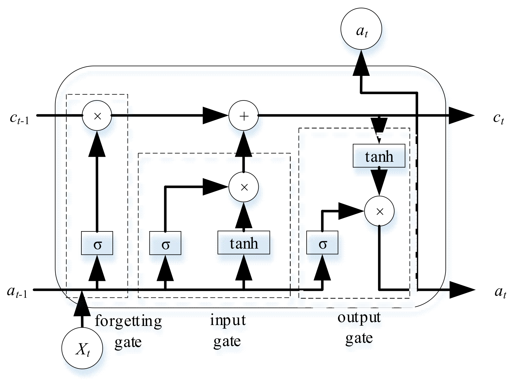
Due to the problems of gradient disappearance and gradient explosion in the traditional recurrent neural network, LSTM neural network was improved. Its internal structure is shown in Figure 1, which is mainly divided into three parts: forgetting gate, input gate and output gate.
The special memory structure makes LSTM neural network has strong memory ability, which is suitable for long time-series-load forecasting. The calculation formula of the three gates of the LSTM neural network is as follows:
- Forgetting gate:
- Input gate:
- Output gate:
For specific meanings of each variable in Formulas (4)–(9), please refer to [20].
3.2. Deep Bidirectional Long and Short-Term Memory Neural Network
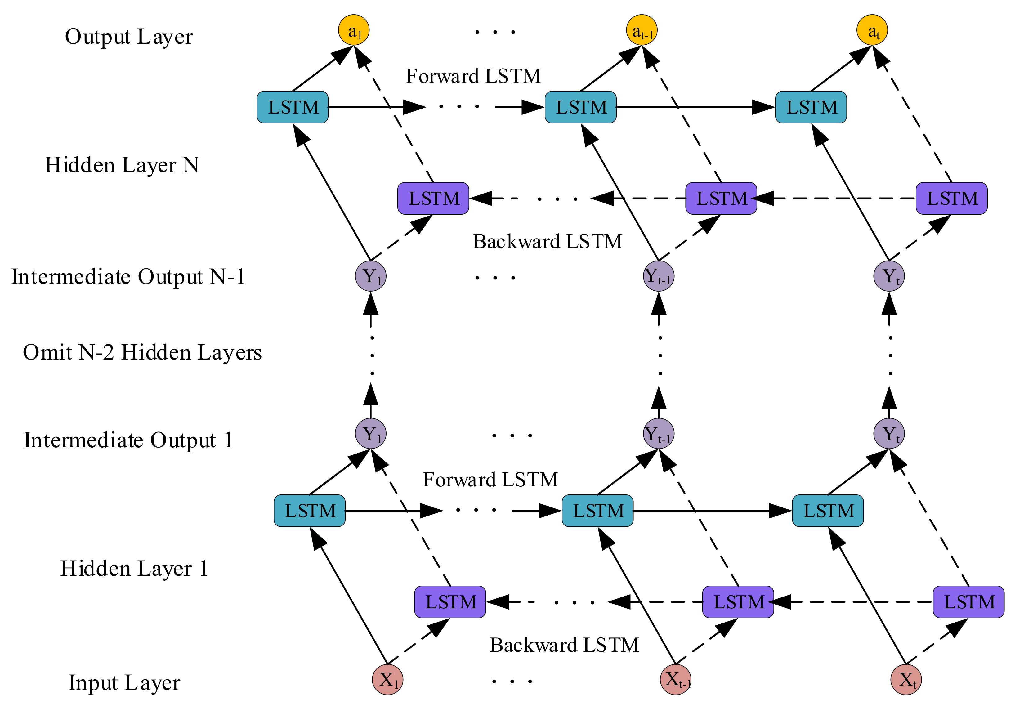
An LSTM neural network makes load forecasting by learning the information contained in load history data. However, the load at the current time is not only related to the load sequence in the previous period but also related to the load sequence in the later period due to the characteristics of the continuity of the load time series. Therefore, the bidirectional long and short-term memory (BiLSTM) neural network is derived from the LSTM neural network.
A BiLSTM neural network is composed of two independent LSTM neural networks, forward and backward. During neural network training, multiple historical loads data and influencing factors selected by Copula correlation analysis together form the input feature set. This input feature set is input to the forward LSTM neural network in the direction of time axis order and input to the backward LSTM neural network in the direction of time axis reverse. The output of each moment is composed of two independent LSTM neural networks. The output of each moment serves as the next neural network layer’s input and is transmitted layer-by-layer to form the DBiLSTM neural network, as shown in Figure 2.
4. Construction of Copula-DBiLSTM Model
4.1. Model Input and Output Settings
Given the great influence of weather factors, such as temperature on multiple loads, and the influence of calendar rules such as hours on multiple loads, the influence factors of weather and calendar rules were selected as feature sets. This was because, for example, when the temperature is high, the use of heat load will decrease, and the use of cooling load will increase. Similarly, because there are many electrical devices for cooling and heating, the electrical load also has a strong relationship with the temperature. The influencing factors of calendar rules also correlate with multiple loads, such as the influencing factor of hours. Since the load curve is a time series, the user’s energy consumption habits show a strong correlation with time, such as greater energy use during the day and less energy use at night.
Since not all factors can play a positive role, the Copula correlation analysis method was used to select effective influencing factors to form the input feature set of the model and the multiple loads, and the output of the model is the multiple loads.
Considering that the multiple loads of the day to be forecasted have a great correlation with the historical loads of the previous week, the electric, cooling, and heating loads of the previous week and various influencing factors selected by Copula were selected as inputs. The output was the electric, cooling and heating loads of the day to be forecasted.
To remove the influence of different dimensional data of different types and improve the training ability of the model, the data were normalized. The specific formula was as follows:
where, and are normalized pre-value and post-value, respectively; and are the minimum and maximum values in the original data sequence, respectively.
4.2. Copula-DBiLSTM Forecasting Model Framework
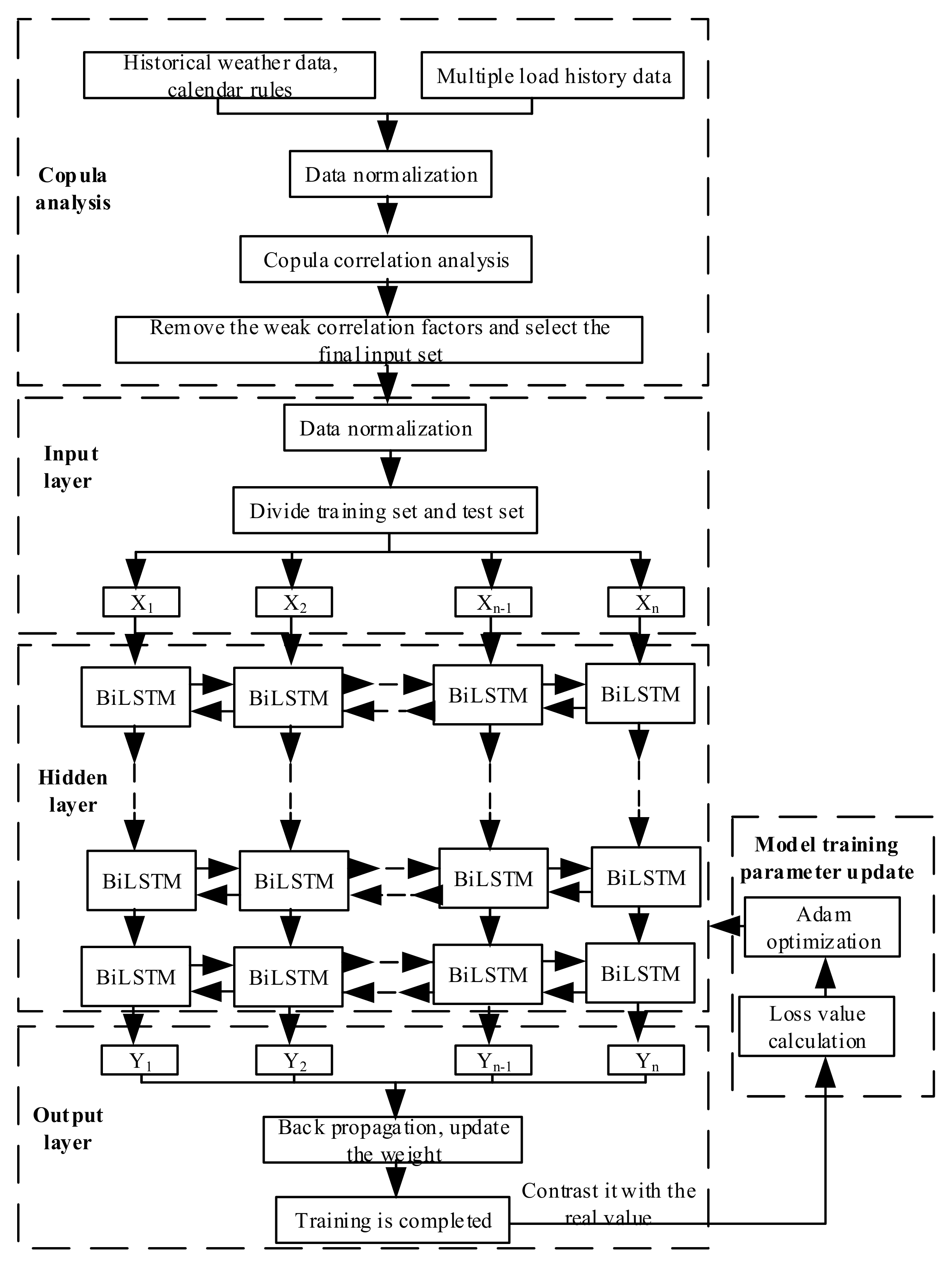
The overall framework of the Copula-DBiLSTM multiple-load forecasting model constructed in this paper is shown in Figure 3. The DBiLSTM neural network made the forecasts after model training on the input feature set composed of historical multiple loads data and influence factors selected by Copula correlation analysis.
By calculating the loss function, combined with the optimization algorithm, the model’s parameters were optimized and updated. Taking the multiple-load forecasting of electric, cooling, and heating loads as an example, the loss function expression was:
where is the value of the loss function; is the number of forecasting points participating in the calculation of the loss value; , , are the actual values of the electric, cooling, and heating loads at time respectively; , , and are the forecasting value of the electric, cooling and heating loads at time respectively.
In this paper, the mean absolute percentage error (), root mean square error (), mean absolute error () and mean square error () were taken as the evaluation indexes of the model forecast results. The expression is as follows:
where is the number of load points participating in the calculation; and are the real and forecasting values at time , respectively.
5. Case Analysis
5.1. Experimental Data Introduction
The experimental data came from the data of the United States IES system from January 2011 to October 2012, with a time resolution of 1 h, including electric, cooling, and heating loads. The corresponding weather data included temperature, humidity, horizontal solar radiation, vertical solar radiation, wind speed, dew point [21]. The calendar rules were months, weeks, days, hours, and holidays. The experimental data were divided into the training set, validation set, and test set according to 8:1:1.
5.2. Copula Correlation Analysis Results
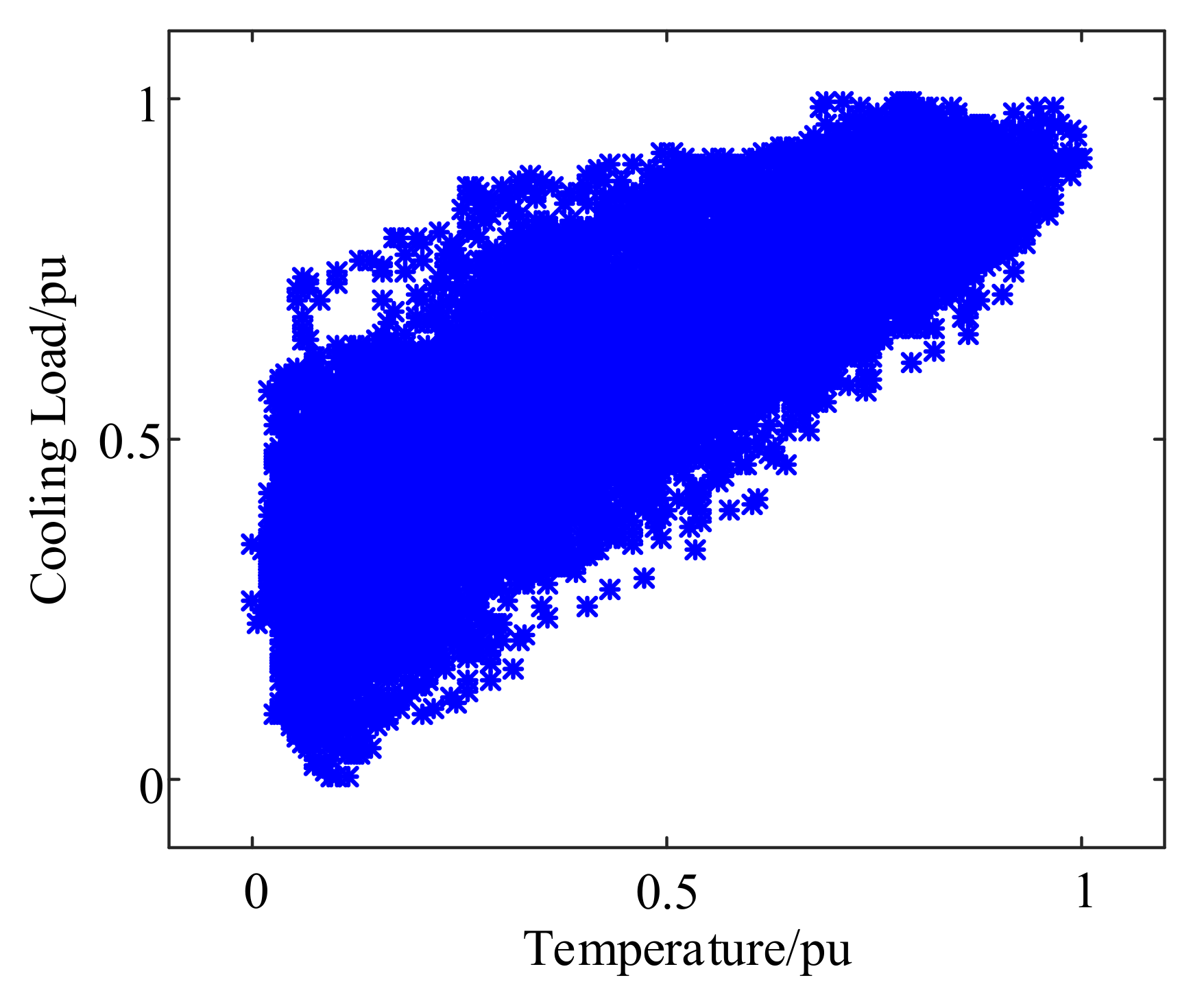
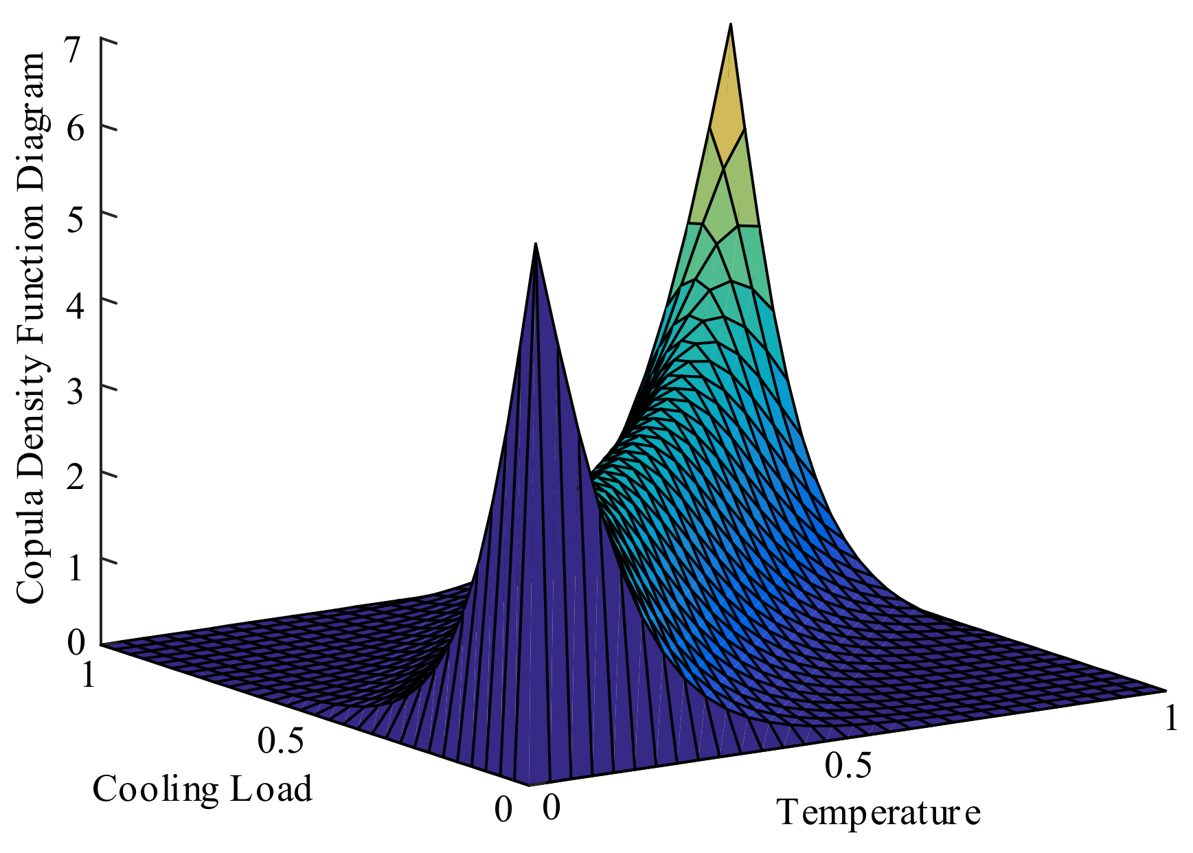
Many influencing factors must be screened through Copula to determine the appropriate input feature set. Figure 4 shows the scatter plot of cooling load and temperature, and Figure 5 shows the probability density function plot of cooling load and temperature. As can be seen from the scatter diagram in Figure 4, the diagram points were all distributed around the 45° diagonal, indicating that the cooling load has a great correlation with temperature. Combined with the Copula density function diagram in Figure 5, it can be seen that the Copula density function diagram of cooling load and temperature presented a diagonal distribution of 45°, with sharp peaks and thick tails at both ends of the diagonal, indicating that there is a great correlation between cooling load and temperature [18].
Although the scatter diagram and the Copula density function diagram above can provide some diagram features to determine the correlation between the two variables, they still lack some intuitiveness. Therefore, Table 1 shows the correlation calculation between the influencing factors of weather and calendar rules and multiple loads by using the Kendall rank correlation coefficient method in Copula.
Since a certain influencing factor may be positively correlated with electric load and negatively correlated with heating load, to comprehensively obtain the correlation between each influencing factor and multiple loads, the definition formula of the average correlation coefficient value is given as follows:
where, represents the average correlation coefficient value between the influencing factor and multiple loads; , and respectively represent the correlation value between the influencing factor and the electric, cooling and heating loads, and is the total number of influencing factors affecting multiple loads.
According to the correlation calculation results in Table 1, the average correlation coefficients between wind speed, holidays, weeks, days and multiple loads were all less than 0.15, which were weakly correlated or even unrelated influencing factors. Given that these four types of influencing factors may lead to a decline in forecasting accuracy, these four types of influencing factors were eliminated. The correlations between the remaining influencing factors and multiple loads were all greater than 0.15, which had a great correlation with multiple loads. The correlation between temperature and multiple loads was the largest, with an average correlation coefficient of 0.5529, which was much higher than other factors. Therefore, the influence factors whose average correlation value was greater than 0.15 were combined with the historical data of electric, cooling and heating loads to form the input feature set of the final model.
As shown in Table 1, there was a strong correlation between electric, cooling and heating loads, so it was necessary to make joint forecasting, verifying the necessity of the multiple-load forecasting model proposed in this paper.
5.3. Model Parameter Setting
We set the optimization algorithm of the DBiLSTM neural network to the Adam optimization algorithm. The learning rate was 0.01, the number of iterations was 150, and the dropout was set to 0.5 to prevent overfitting. After many experiments, the number of hidden layers of the neural network was finally selected as 2 layers. The number of neurons in each hidden layer was 50 and 100, respectively.
5.4. Analysis of Copula-DBiLSTM Forecasting Results
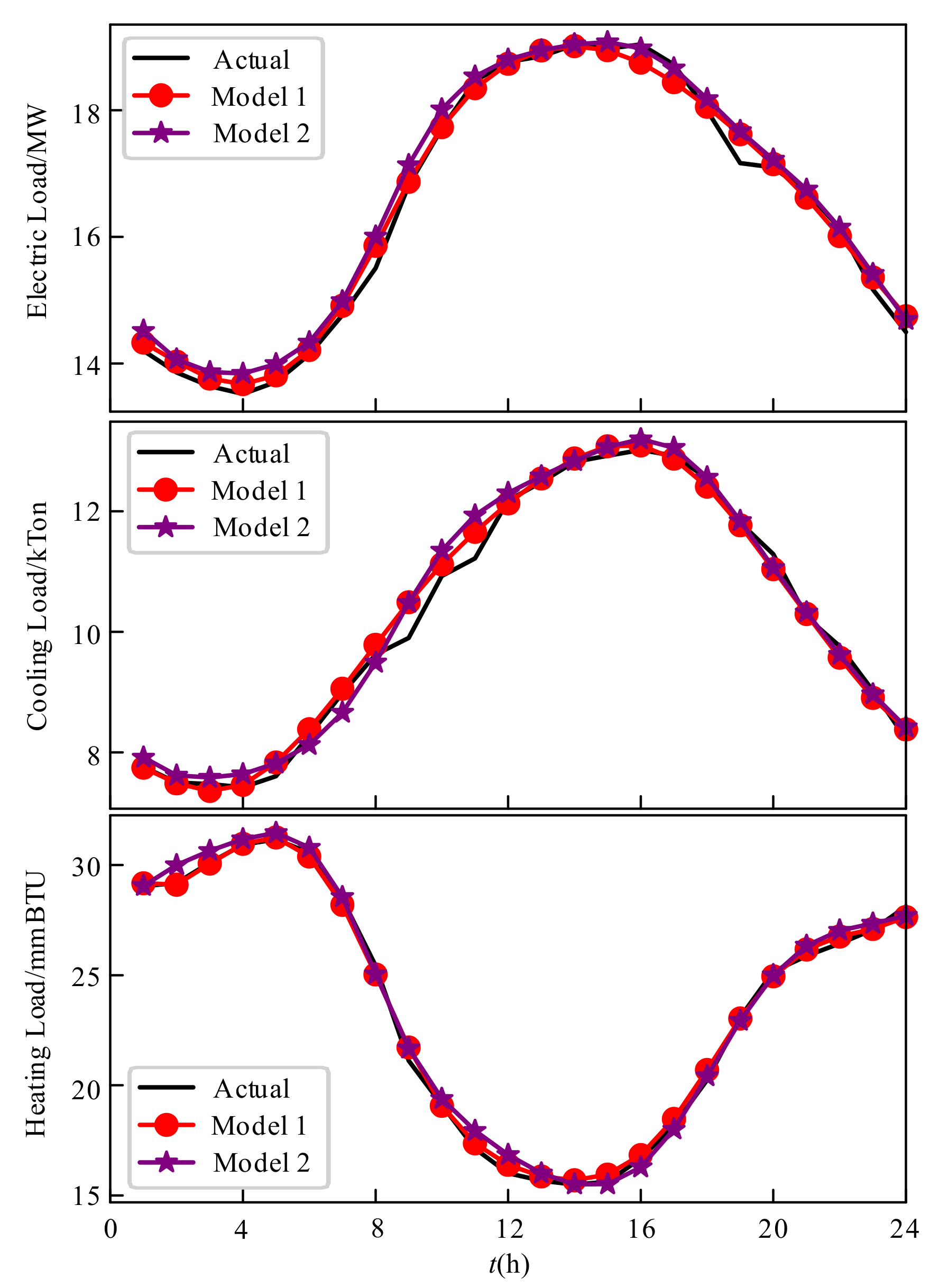
To verify the effectiveness of the Copula-DBiLSTM forecasting model proposed in this paper, the influence factors of weather and calendar rules were considered. The input feature set constructed by using Copula correlation (model 1), and the input set constructed by not using Copula correlation (model 2) were compared. The forecasting results on 21 September 2012 were selected for display. The results are shown in Figure 6 and Table 2.
It can be seen that after considering the application of Copula correlation analysis to select the influencing factors, the forecasting result was better. Combined with the correlation analysis in Table 1, it could be seen that due to the interference of weakly correlated or unrelated factors, like wind speed, taking these influencing factors as the input feature set of the model will reduce the forecasting performance of the model. By using the Copula correlation analysis method to screen out the influential factors with a strong correlation with multiple loads as the input feature set of the model, the influence of interference factors could be removed, which improved the forecasting accuracy of the model.
5.5. Comparative Analysis of Different Models
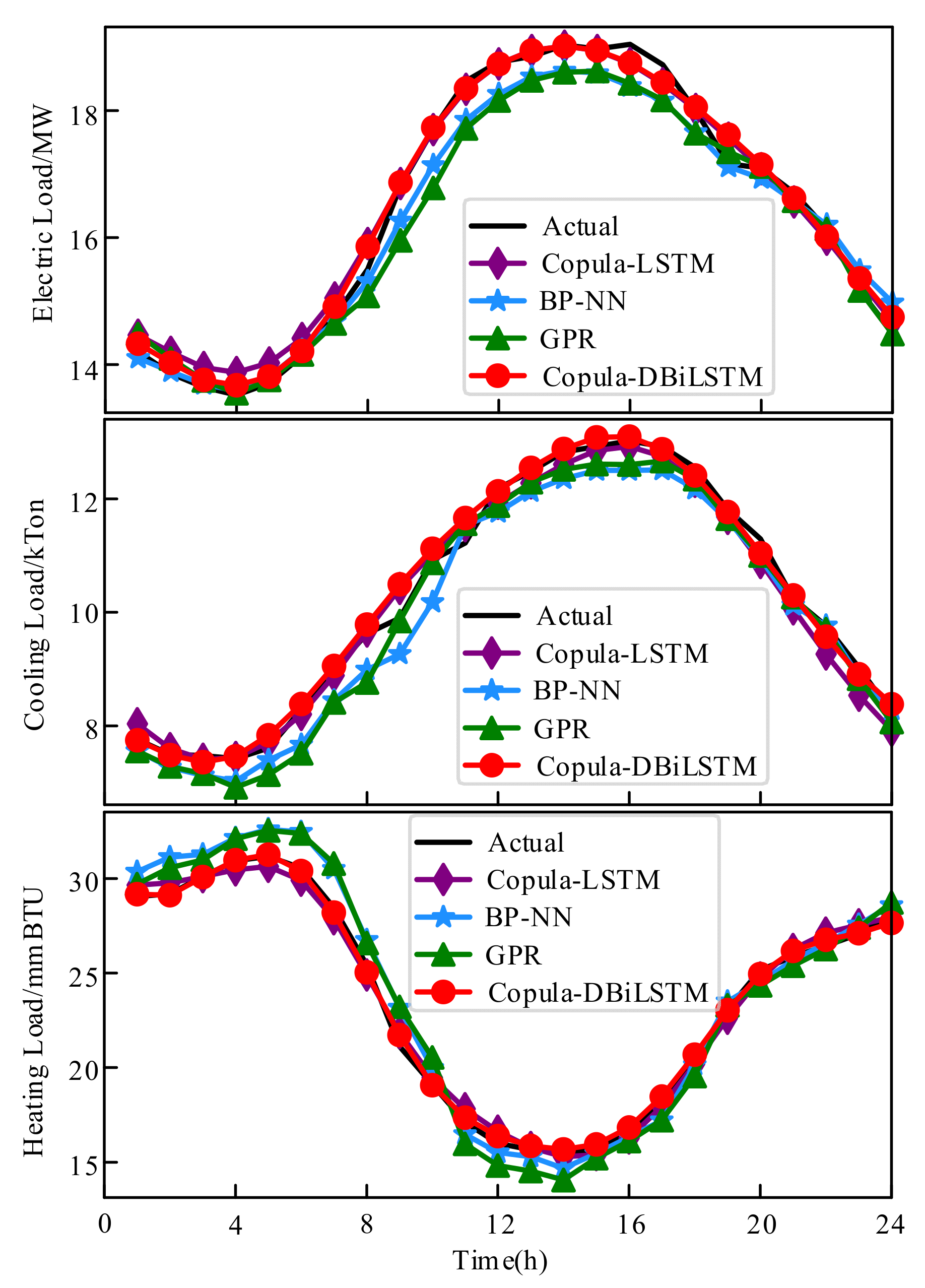
The proposed model in this paper was compared with several commonly used models, including Gaussian process regression (GPR) [22], BP neural network (BP-NN), Copula combined with LSTM neural network (Copula-LSTM). The results are shown in Figure 7 and Table 3.
Combined with Figure 7 and Table 3, on the whole, the traditional forecasting model GPR had the worst error indexes. Compared with GPR, the BP-NN model showed some improvement, but the forecasting accuracy was also limited. Compared with the above two models, the Copula correlation analysis method combined with the deep learning LSTM neural network was greatly improved the forecasting accuracy. The error indexes of electric, cooling and heating loads were only 69.7%, 65.8% and 40.9% of GPR, respectively. However, the forecasting model proposed in this paper had the best effect, and the error indexes of electric, cooling and heating loads were only 71.8%, 67.3% and 57.0% of Copula-LSTM, and 50.0%, 44.3% and 23.3% of GPR, respectively. At the same time, by observing the remaining three error indicators, we concluded that the forecasting model proposed in this paper had the best effect, and the forecasting accuracy was higher than other models.
Further analysis shows that:
- GPR was only applicable to small-scale data and required relatively high regularity of data, so the forecasting effect was the worst;
- Although the forecasting result of BP-NN was better than that of GPR, the performance of the model was also poor due to the inability to remember the information of long time-series and the tendency of gradient disappearance or gradient explosion;
- In the Copula-LSTM model, LSTM neural network could improve the problems of the traditional neural networks, such as gradient disappearance, and its internal structure had a memory unit, which was very suitable for learning long time series. Therefore, compared with the above two models, the forecasting accuracy was greatly improved. However, LSTM neural network only conducted one-way learning on historical data, so it could not effectively learn more information contained in historical data;
- The model proposed in this paper comprehensively considered the impact of weather and calendar rules on the multiple loads. Through Copula correlation analysis, the optimal feature set was selected as the input of the model and combined with the DBiLSTM neural network. It could learn historical data from both forward and backward directions. The model could learn more useful information, and the forecasting accuracy showed a certain improvement compared with the above model.
5.6. Comparison of Different Neural Network Structures
To compare the influence of different neural network structures on the prediction accuracy, the number of hidden layers and the number of neurons of different neural networks were analyzed experimentally. The results are shown in Table 4 and Table 5.
It can be seen from Table 4 and Table 5 that when the neural network had two hidden layers, and the number of neurons in each hidden layer was 50 and 100, respectively, the forecasting effect was the best.
The results show that when the structure of the neural network was too simple, it could not fit the historical data well. At the same time, the increased complexity of the neural network structure did not fit the data better. This was because more neural network layers increased more parameters to be optimized, which in turn made the model more difficult to train, and may have caused “overfitting” phenomena, resulting in the forecasting accuracy not being improved. In addition, the more hidden layers, the higher were the time costs of training.
5.7. Comparison of Single Load Forecasting and Multiple Load Forecasting
To illustrate the effectiveness of multiple-load forecasting, a comparative analysis of single-load and multiple-load forecasting was carried out. The model input did not consider the other two load factors in single-load forecasting. The results are shown in Table 6.
As seen in Table 6, the result of single-load forecasting was worse than that of multiple-load forecasting. In combination with Table 1, it can be seen that there was an obvious coupling relationship between electric, cooling and heating loads, with a strong correlation. Taking the other two load factors into consideration in the forecasting could enable the model to learn more useful information and thus improve the forecasting accuracy.
At the same time, because the multiple-load forecasting model could obtain the forecasting resulted of multiple loads at one time, compared to the single-load forecasting that requires three forecasting models to be constructed, the time-consuming cost was lower. Therefore, in terms of forecasting accuracy and time-consuming cost, multiple-load forecasting had greater advantages.
6. Conclusions
In this paper, a Copula-DBiLSTM multiple-load forecasting model was proposed. The Copula correlation analysis method was used to select the input feature set of the forecasting model, and the DBILSTM neural network was used to make the forecasting. By comparing with other models, the following conclusions were drawn:
- The Copula correlation analysis method was used to screen out the influencing factors with greater correlation with the multiple loads as the input feature set of the model, which could construct a suitable input feature set, eliminate the influence of interference factors, and improve the forecasting accuracy of the model;
- The DBiLSTM neural network was suitable for long-term sequence forecasting, and due to its unique bidirectional learning advantage of historical data; it could learn the useful information contained in historical data more comprehensively;
- Due to the close coupling of multiple loads in the IES system, the multiple load forecasting model considered the influence of the other two loads compared with the single-load forecasting model so that the model could learn more useful information. Moreover, the time-costs of a multiple-load forecasting model were lower than that of a single-load forecasting model because there was no need to forecast all kinds of loads independently. Hence, it had many advantages.
On the basis of the research in this paper, the author proposes the following directions that could be continued in the future:
- Due to the close coupling of multiple energy sources within IES, the system was affected by real-time electricity prices, gas prices and other factors during optimized operation. At the same time, these price factors will also affect users’ energy consumption habits. Therefore, price factors could be considered in the input feature set to construct a more suitable input feature set;
- Since the selection of the number of hidden layers and neurons of the neural network was determined based on several experiments, the subsequent research could find some methods to optimize these parameters.
- Since the intelligent terminal equipment may produce abnormal data or missing data in the process of data collection, the identification of abnormal data and the supplement of missing data before model training is also a direction worthy of further research.
Author Contributions
Conceptualization, J.Z. and L.Z.; methodology, J.Z. and J.C.; validation, S.N.; formal analysis, G.W.; investigation, C.W.; resources, Z.C.; data curation, J.C.; writing—original draft preparation, J.C.; writing—review and editing, J.C. and J.Z.; visualization, J.Z.; supervision, Z.H. All authors have read and agreed to the published version of the manuscript.
Funding
This work was supported by the national natural science foundation of China (51977156) and the science and technology project of Economic Technology Research Institute, State Grid Fujian Electric Power Co., Ltd. (52130N19000P).
Institutional Review Board Statement
Not applicable.
Informed Consent Statement
Not applicable.
Data Availability Statement
The data presented in this study are available on request from the corresponding author.
Conflicts of Interest
The authors declare no conflict of interest.
References
- Chaaraoui, S.; Bebber, M.; Meilinger, S.; Rummeny, S.; Schneiders, T.; Sawadogo, W.; Kunstmann, H. Day-Ahead Electric Load Forecast for a Ghanaian Health Facility Using Different Algorithms. Energies 2021, 14, 409. [Google Scholar] [CrossRef]
- Chen, W.N.; Hu, Z.J.; Yue, J.P.; Du, Y.X.; Qi, Q. Short-term load prediction based on combined model of long short-term memory network and light gradient boosting machine. Autom. Electr. Power Syst. 2021, 45, 91–97. [Google Scholar]
- Sun, Q.K.; Wang, X.J.; Zhang, Y.Z.; Zhang, F.; Zhang, P.; Gao, W.Z. Multiple load prediction of integrated energy system based on LSTM-MTL. Autom. Electr. Power Syst. 2021, in press. [Google Scholar]
- Ma, H.; Chen, Q.; Hu, B.; Sun, Q.; Li, T.; Wang, S. A compact model to coordinate flexibility and efficiency for decomposed scheduling of integrated energy system. Appl. Energy 2021, 285, 116474. [Google Scholar] [CrossRef]
- Hwang, J.S.; Fitri, I.R.; Kim, J.-S.; Song, H. Optimal ESS Scheduling for Peak Shaving of Building Energy Using Accuracy-Enhanced Load Forecast. Energies 2020, 13, 5633. [Google Scholar] [CrossRef]
- Zheng, Z.; Chen, H.; Luo, X. A Kalman filter-based bottom-up approach for household short-term load forecast. Appl. Energy 2019, 250, 882–894. [Google Scholar] [CrossRef]
- Lopez, J.C.; Rider, M.J.; Wu, Q. Parsimonious Short-Term Load Forecasting for Optimal Operation Planning of Electrical Distribution Systems. IEEE Trans. Power Syst. 2019, 34, 1427–1437. [Google Scholar] [CrossRef] [Green Version]
- Aprillia, H.; Yang, H.-T.; Huang, C.-M. Optimal Decomposition and Reconstruction of Discrete Wavelet Transformation for Short-Term Load Forecasting. Energies 2019, 12, 4654. [Google Scholar] [CrossRef] [Green Version]
- Li, Y.; Che, J.; Yang, Y. Subsampled support vector regression ensemble for short term electric load forecasting. Energy 2018, 164, 160–170. [Google Scholar] [CrossRef]
- Mayur, B.; Nalin, B.D.C. Season specific approach for short-term load forecasting based on hybrid FA-SVM and similarity concept. Energy 2019, 174, 886–896. [Google Scholar]
- Liu, D.; Sun, K. Random forest solar power forecast based on classification optimization. Energy 2019, 187, 115940. [Google Scholar] [CrossRef]
- Wang, Z.; Hong, T.; Piette, M.A. Building thermal load prediction through shallow machine learning and deep learning. Appl. Energy 2020, 263, 114683. [Google Scholar] [CrossRef] [Green Version]
- Niu, Z.; Yu, Z.; Tang, W.; Wu, Q.; Reformat, M. Wind power forecasting using attention-based gated recurrent unit network. Energy 2020, 196, 117081. [Google Scholar] [CrossRef]
- Zhang, X.; Chan, K.W.; Li, H.; Wang, H.; Qiu, J.; Wang, G. Deep-Learning-Based Probabilistic Forecasting of Electric Vehicle Charging Load With a Novel Queuing Model. IEEE Trans. Cybern. 2020, 99, 1–14. [Google Scholar] [CrossRef]
- Cao, Z.; Wan, C.; Zhang, Z.; Li, F.; Song, Y. Hybrid Ensemble Deep Learning for Deterministic and Probabilistic Low-Voltage Load Forecasting. IEEE Trans. Power Syst. 2020, 35, 1881–1897. [Google Scholar] [CrossRef]
- Li, R.; Sun, F.; Ding, X.; Han, Y.; Liu, Y.P.; Yan, J.R. Ultra short-term load forecasting for user-level integrated energy system considering multi-energy spatio-temporal coupling. Power Syst. Technol. 2020, 44, 4121–4134. [Google Scholar]
- Zhu, R.; Guo, W.; Gong, X. Short-Term Load Forecasting for CCHP Systems Considering the Correlation between Heating, Gas and Electrical Loads Based on Deep Learning. Energies 2019, 12, 3308. [Google Scholar] [CrossRef] [Green Version]
- Yang, X.; Chen, B.C.; Zhu, L.; Fang, C. Short-term public building load probability density prediction based on correlation analysis and long- and short-term memory network quantile regression. Power Syst. Technol. 2019, 43, 3061–3071. [Google Scholar]
- Wan, J.H.; Su, H.; Feng, D.H.; Zhao, Y.; Fan, Y.; Yu, B. Analysis and evaluation of the complementarity characteristics of wind and photovoltaic considering source-load matching. Power Syst. Technol. 2020, 44, 3219–3226. [Google Scholar]
- Chen, J.P.; Hu, Z.J.; Chen, W.N.; Gao, M.X.; Du, Y.X.; Lin, M.R. Load prediction of integrated energy system based on quadratic modal decomposition and DBiLSTM-MLR. Autom. Electr. Power Syst. 2021, in press. [Google Scholar]
- NSRDB Data Viewer. Available online: https://maps.nrel.gov/nsrdb-viewer/ (accessed on 25 November 2020).
- Li, F.; Li, C.Y.; Yang, Y.; Yan, Q.Q.; Zhao, J.B.; Wang, L.J. Short-term photovoltaic power probability forecasting based on OLPP-GPR and modified clearness index. J. Eng. 2017, 1, 1625–1628. [Google Scholar]
Figure 1.
Internal structure diagram of long and short-term memory (LSTM) neural network.

Figure 2.
Structure diagram of deep bidirectional long and short-term memory (DBiLSTM) neural network.
Figure 2.
Structure diagram of deep bidirectional long and short-term memory (DBiLSTM) neural network.

Figure 3.
Based on the overall framework of Copula-DBiLSTM neural network model.

Figure 4.
Scatter diagram of cooling load and temperature.

Figure 5.
Copula density function diagram of cooling load and temperature.

Figure 6.
Comparison of results under different input feature sets.

Figure 7.
Comparison of results under different models.


Table 1.
The correlation value between each factor.
| Influencing Factors | Electric Load | Cooling Load | Heating Load | Average Correlation Coefficient |
|---|---|---|---|---|
| Electric load | 1.0000 | 0.3317 | −0.3209 | 0.5509 |
| Cooling load | 0.3317 | 1.0000 | −0.7737 | 0.7018 |
| Heating load | −0.3209 | −0.7737 | 1.0000 | 0.6982 |
| Temperature | 0.2778 | 0.6694 | −0.7114 | 0.5529 |
| Wind speed | 0.1239 | 0.0591 | −0.1254 | 0.1028 |
| Humidity | −0.2451 | −0.2789 | 0.4180 | 0.3140 |
| Direct normal irradiance | 0.3651 | 0.1957 | −0.3521 | 0.3043 |
| Global horizontal irradiance | 0.3843 | 0.2528 | −0.4098 | 0.3490 |
| Dew point | 0.0800 | 0.3778 | −0.2717 | 0.2432 |
| Holidays | −0.0481 | −0.0261 | 0.0299 | 0.0347 |
| Months | 0.1714 | 0.3348 | −0.2447 | 0.2503 |
| Weeks | −0.2113 | −0.0295 | 0.0004 | 0.0804 |
| Days | 0.0164 | 0.0303 | −0.0296 | 0.0254 |
| Hours | 0.2823 | 0.1365 | −0.1237 | 0.1808 |
Table 2.
Error comparison under different input feature sets.
| Model | EMAPE | ERMSE | EMAE | EMSE | ||||||||
|---|---|---|---|---|---|---|---|---|---|---|---|---|
| Electric (%) | Cooling (%) | Heating (%) | Electric (MW) | Cooling (kTon) | Heating (mmBTU) | Electric (MW) | Cooling (kTon) | Heating (mmBTU) | Electric (MW2) | Cooling (kTon2) | Heating (mmBTU2) | |
| Model 1 | 0.89 | 1.40 | 1.06 | 0.179 | 0.193 | 0.274 | 0.142 | 0.141 | 0.226 | 0.032 | 0.037 | 0.075 |
| Model 2 | 1.25 | 1.95 | 1.59 | 0.238 | 0.253 | 0.423 | 0.194 | 0.191 | 0.349 | 0.057 | 0.064 | 0.179 |
Table 3.
Error comparison under different models.
| Model | EMAPE | ERMSE | EMAE | EMSE | ||||||||
|---|---|---|---|---|---|---|---|---|---|---|---|---|
| Electric (%) | Cooling (%) | Heating (%) | Electric (MW) | Cooling (kTon) | Heating (mmBTU) | Electric (MW) | Cooling (kTon) | Heating (mmBTU) | Electric (MW2) | Cooling (kTon2) | Heating (mmBTU2) | |
| Copula-DBiLSTM | 0.89 | 1.40 | 1.06 | 0.179 | 0.193 | 0.274 | 0.142 | 0.141 | 0.226 | 0.032 | 0.037 | 0.075 |
| GPR | 1.78 | 3.16 | 4.55 | 0.417 | 0.366 | 1.157 | 0.310 | 0.301 | 1.016 | 0.174 | 0.134 | 1.338 |
| BP-NN | 1.64 | 3.59 | 3.69 | 0.353 | 0.409 | 1.087 | 0.283 | 0.363 | 0.893 | 0.124 | 0.167 | 1.181 |
| Copula-LSTM | 1.24 | 2.08 | 1.86 | 0.233 | 0.255 | 0.476 | 0.190 | 0.210 | 0.426 | 0.054 | 0.065 | 0.227 |
Table 4.
Comparison of forecasting results with different hidden layers.
| Number of Hidden Layers | EMAPE | Training Time (s) | ||
|---|---|---|---|---|
| Electric (%) | Cooling (%) | Heating (%) | ||
| 1 | 1.91 | 2.35 | 2.34 | 536.49 |
| 2 | 0.89 | 1.40 | 1.06 | 706.12 |
| 3 | 1.20 | 2.05 | 4.49 | 994.98 |
| 4 | 1.68 | 3.62 | 3.42 | 1487.32 |
Table 5.
Comparison of forecasting results of different numbers of neurons in 2 hidden layers.
| Number of Hidden Layers | EMAPE | Training Time (s) | ||
|---|---|---|---|---|
| Electric (%) | Cooling (%) | Heating (%) | ||
| 32/64 | 1.64 | 2.17 | 2.37 | 565.38 |
| 50/100 | 0.89 | 1.40 | 1.06 | 706.12 |
| 64/128 | 1.54 | 1.89 | 1.99 | 892.67 |
| 100/200 | 1.79 | 2.07 | 2.57 | 1200.98 |
Table 6.
Error comparison between single-load and multiple-load forecasting.
| Model | EMAPE | Time | |||
|---|---|---|---|---|---|
| Electric (%) | Cooling (%) | Heating (%) | Training (s) | Forecast (s) | |
| Single-load forecasting | 1.14 | 1.96 | 2.04 | 2105.08 | 26.67 |
| Multiple-load forecasting | 0.89 | 1.40 | 1.06 | 706.12 | 9.24 |
Publisher’s Note: MDPI stays neutral with regard to jurisdictional claims in published maps and institutional affiliations. |
© 2021 by the authors. Licensee MDPI, Basel, Switzerland. This article is an open access article distributed under the terms and conditions of the Creative Commons Attribution (CC BY) license (https://creativecommons.org/licenses/by/4.0/).
Share and Cite
MDPI and ACS Style
Zheng, J.; Zhang, L.; Chen, J.; Wu, G.; Ni, S.; Hu, Z.; Weng, C.; Chen, Z. Multiple-Load Forecasting for Integrated Energy System Based on Copula-DBiLSTM. Energies 2021, 14, 2188. https://0-doi-org.brum.beds.ac.uk/10.3390/en14082188
AMA Style
Zheng J, Zhang L, Chen J, Wu G, Ni S, Hu Z, Weng C, Chen Z. Multiple-Load Forecasting for Integrated Energy System Based on Copula-DBiLSTM. Energies. 2021; 14(8):2188. https://0-doi-org.brum.beds.ac.uk/10.3390/en14082188
Chicago/Turabian StyleZheng, Jieyun, Linyao Zhang, Jinpeng Chen, Guilian Wu, Shiyuan Ni, Zhijian Hu, Changhong Weng, and Zhi Chen. 2021. "Multiple-Load Forecasting for Integrated Energy System Based on Copula-DBiLSTM" Energies 14, no. 8: 2188. https://0-doi-org.brum.beds.ac.uk/10.3390/en14082188
Note that from the first issue of 2016, this journal uses article numbers instead of page numbers. See further details here.