
Dynamic Prospective Average and Marginal GHG Emission Factors—Scenario-Based Method for the German Power System until 2050


Institute of Energy Economics and Rational Energy Use (IER), University of Stuttgart, 70565 Stuttgart, Germany
*
Author to whom correspondence should be addressed.
Energies 2021, 14(9), 2527; https://0-doi-org.brum.beds.ac.uk/10.3390/en14092527
Submission received: 26 February 2021
/
Revised: 12 April 2021
/
Accepted: 21 April 2021
/
Published: 28 April 2021
Abstract
:Due to the continuous diurnal, seasonal, and annual changes in the German power supply, prospective dynamic emission factors are needed to determine greenhouse gas (GHG) emissions from hybrid and flexible electrification measures. For the calculation of average emission factors (AEF) and marginal emission factors (MEF), detailed electricity market data are required to represent electricity trading, energy storage, and the partial load behavior of the power plant park on a unit-by-unit, hourly basis. Using two normative scenarios up to 2050, different emission factors of electricity supply with regard to the degree of decarbonization of power production were developed in a linear optimization model through different GHG emission caps (Business-As-Usual, BAU: −74%; Climate-Action-Plan, CAP: −95%). The mean hourly German AEF drops to 182 gCO2eq/kWhel (2018: 468 gCO2eq/kWhel) in the BAU scenario by the year 2050 and even to 29 gCO2eq/kWhel in the CAP scenario with 3700 almost emission-free hours from power supply per year. The overall higher MEF decreases to 475 and 368 gCO2eq/kWhel, with a stricter emissions cap initially leading to a higher MEF through more gas-fired power plants providing base load. If the emission intensity of the imported electricity differs substantially and a storage factor is implemented, the AEF is significantly affected. Hence, it is not sufficient to use the share of RES in net electricity generation as an indicator of emission intensity. With these emission factors it is possible to calculate lifetime GHG emissions and determine operating times of sector coupling technologies to mitigate GHG emissions in a future flexible energy system. This is because it is decisive when lower-emission electricity can be used to replace fossil energy sources.
1. Introduction
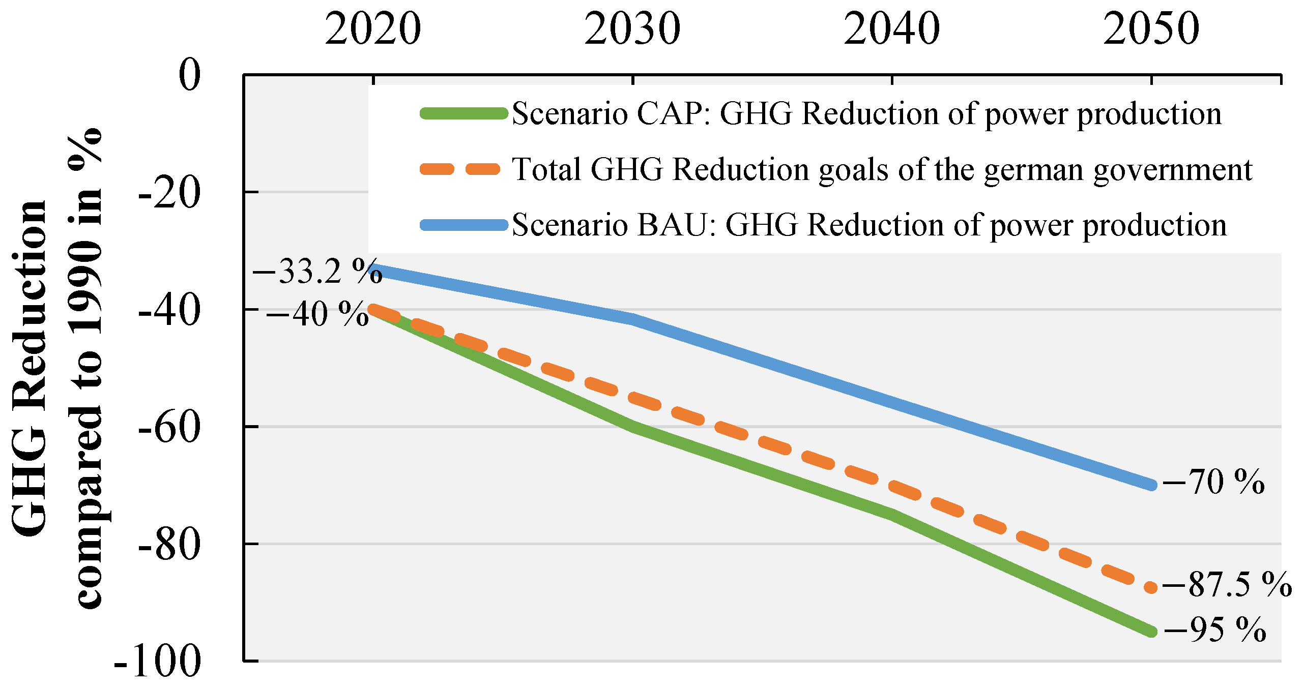
The main driver of the continuous rise in the Earth’s temperature is the increase in the concentration of greenhouse gases in the atmosphere, of which carbon dioxide is the most significant [1]. The German government has developed a climate action plan that stipulates a reduction in GHG emissions of 80 to 95% by 2050, compared with 1990 levels [2].
The electric power industry is one of the largest emitters of GHG worldwide [3]. In 2018, 269 million tons of carbon dioxide (CO2) emissions were released in Germany as a result of the combustion of energy sources to generate electricity. As the share of renewable energy sources (RES) in net power production (NPP) has increased to 41% in 2018, absolute and specific CO2 emissions have decreased [4]. The specific emission factor of electricity supply is 31% lower in 2018 at 468 gCO2/kWhel than in 1990 at 764 gCO2/kWhel [5]. Preliminary data show a further decrease of the emission factor to about 401 gCO2/kWhel in 2019 and a continuing increase of the share of RES in NPP to approximately 51% in 2020 [5,6].
The environmental impact or carbon footprint of power supply is often analyzed through a life cycle assessment using GHG emission factors. In the scope definition, the functional unit, geographical and temporal boundaries, and the attributive or consequential perspective are defined. The following inventory analysis collects information about the physical flows in terms of input of resources and, for example, the output of the emissions [7]. Often, as in the case of electromobility, the use phase of a product is the sub-process with the most significant impact on GHG [8,9]. Therefore, in this paper we want to analyze the direct GHG emissions resulting from the electricity supply.
Because of the production of electricity with a mixed power plant park in Germany, the emission factor of power production fluctuates continuously. This is due to the growing share of fluctuating RES, such as photovoltaic and wind power plants, in power production and the German coal phase-out by 2038 [10]. The future energy supply system must therefore be flexible, both on the supply side and on the demand side [11]. This development will increase seasonal and diurnal fluctuations and cause an overall decrease in emission factors [12]. For the assessment, GHG emissions of consumers with fluctuating energy demand emission factors that vary over time must be used. The effects of demand-side management, efficiency measures, or the expansion of RES on the emissions can only be examined in detail with dynamic emission factors [13,14,15]. This necessity of varying emission factors is clearly shown in previous studies by [8,12,16,17,18,19]. A significant error is made when the yearly average emission factor is used for the ecological assessment as long as the demand for electricity is not constant for every hour of a year [20,21]. In this paper we develop prospective hourly emission factors for the German power supply. First, we identify the various methodologies and interpretations of power supply emission factors. Then we look at the publications of emission factors for the German electricity supply and where their shortcomings lie.
A fundamental decision in defining the emission factor for power production is the one between the electricity mix and the marginal emission factor [22]. The system-average emission factor method takes into account all emissions from the power-generating plants that produce to meet demand in the area under consideration with or without exchanged power [23]. In scenario-based emission models, the AEF is often calculated using the average emission factors of the generating power plant types, weighted according to the share of demand met by each power plant type, for each time interval [22]. The AEF is most commonly used in studies where the emission savings are a side effect of energy savings from any kind of technoeconomic measures [24]. According to [23], the AEF is correctly applied when the load to be analyzed is part of the existing demand or when the consequences of an existing electricity use are to be calculated. However, if the load to be analyzed represents a new change in demand, the use of MEFs is recommended [23]. If the new future demand is taken into account in the planning of power production, according to [25], then the AEF can also be used for this new demand. The authors of [26] conclude that the calculation of the emission factor should always be based on net power consumption rather than on power production, otherwise the results may be misinterpreted when applying the factors. The GHG emissions presented by the AEF in this paper are thus based on the net power consumption. Net power consumption is defined as gross power production plus imports and minus exports, auxiliary consumption, pumping, and grid losses.
The MEF is used to determine the impact of a change in demand. The MEF represents the emissions generated by the reacting generation units due to the change in demand and is usually considerably higher than the AEF [27,28].
The general power supply system is a highly interconnected network in which electricity is supplied by various producers to different locations in the area of supply. The system is dynamic and responds to economic signals (e.g., fuel and stock exchange prices), technical restrictions (e.g., start-up times and frequency control), and transmission constraints [29]. The challenge is therefore to identify which power plants respond to changes in demand at a given point in time and to what extent (marginal electricity mix or marginal power plant) [27]. In contrast to the AEF, the MEF approach is an ecological assessment method that more realistically reflects the response of the power generation system [30].
Some of the established methods for calculating the MEF are divided into two groups, the “top-down” and the “bottom-up” approaches [29]. In the first group, the normative economic behavior of power plants in the event of a change in demand is examined. For this purpose, a permanent marginal power plant can be defined in a simple manner, to which the entire change in demand is attributed, or a merit order of the power plants employed can be formed [31]. However, more than just one generation unit, but not all of them as in the case of the AEF, reacts to changes in demand. Because of grid restrictions or must-run feed-in, the generating units do not always react according to the theoretical merit order [23,30,32].
The second group of methods comprises the top-down approaches. Simulation or optimization models (electricity market models) are often used to assess the effects of load changes when investigating future emission factors in order to capture the effects of the entire power generation system. For a consideration of long-term changes, such as new power plant construction and its dispatch, two scenarios are formed in energy system models with a shifted demand. The principle of this approach is to investigate the effects of a shifted load or demand in simulation or optimization models under otherwise constant input parameters but dynamic conditions [8]. Böing and Regett, Pehnt et al., and Klobasa and Sensfuß demonstrate this methodology for Germany [33,34,35]. For the creation of detailed and complex energy system models, a considerable number of parameters and input data have to be defined and many assumptions have to be made in order to obtain reproducible results [36]. The associated computing and workload are huge, and depending on the complexity of the investigation, not feasible and not necessarily practicable for LCA [37,38].
Another less-complex methodology in the top-down approach is that of the average MEF using the linear regression method, which is used in this paper. References [27,30] calculate the difference between two consecutive hours from the amount of conventional (fossil) power generation and the emissions produced. From the linear regression of the difference in emissions over the difference in conventional power generation, the gradient of the fitted regression line is calculated, which can be assumed to be a reasonable approximation of the average MEF [30]. This approach works on the assumption that the marginal power generators are always conventional fossil-fueled power plants, because renewable energies are usually fluctuating, except bioenergy and some hydropower plants, and are subject to feed-in priority [36,39]. The average MEF can be further specified by time- or load-dependent classification (binning) [30,36].
In addition, the MEF can be divided into a direct (short-term) and indirect (long-term) MEF. The latter describes the effects of changes in demand on the composition of the future power plant park. In this paper, a direct MEF is formed which does not consider changes in the composition of the power plant park in the long term. This is due to the fact that the development of the generated scenarios is predetermined on the basis of national expansion plans, such as the German nuclear and coal phase-out, and the promotion of renewable energies and their regulated expansion volumes (tendering mechanism).
There are significant discrepancies in the choice of system boundaries, depth of investigation and the distinction between the average electricity mix (AEF) and a marginal emission factor (MEF) when determining the “appropriate” emission factor. Furthermore, different methods of allocation (for cogeneration) and different fuel-based emission factors can be used to calculate the emissions of the combusted energy source, depending on the composition and the consideration of the upstream processes of the fuels. An overview of the different methods and the application of the factors for the evaluation of electrical appliances is further described in [8,22,23].
In an empirical context and with lower temporal resolution, the AEF and MEF are rather easy to determine. The need for at least hourly resolved emission factors of electricity supply (AEF) combined with analyses based on historical market data have already been shown by [13,17,40]. Historical hourly emission factors to evaluate emission saving measures have been used in the areas of load shifting [20,41], energy efficiency measures in buildings [16], emission reduction in households [13], smart-home solutions [42], electromobility [39,43,44,45], and emission reduction through the use of RES in power production [15,46,47]. The analysis and application of hourly emission factors for Germany was carried out by [12,18,39,48] from the respective current structure of power production derived from empirical data. The authors of [49] determined an AEF and an indicator-based MEF for Germany derived from the merit order of the power plants from an electricity market model, as well as an annual and an hourly MEF using the linear regression method according to [30]. These emission factors from historical data are used for the ecological assessment and dispatch of battery storage systems. The authors of [19] showed that it is essential for the development of low-emission local energy systems in Germany to use dynamic, rather than constant, emission factors of power production. This is the only way to achieve the emission reduction intended by sector coupling, by correctly planning the use of flexible and hybrid technologies.
In addition to the current hourly emission factor, which is important for an accurate ecological assessment, the emission factor of future electricity supply is also required for the calculation of emissions over the entire lifetime of an electricity-using technology. Prospective emission factors with high temporal resolution are calculated, for example, by [32] for England and by [45] for California.
A future consideration of the emission factors for Germany was calculated by [50] using capacity factors and the planned installed capacity from two different scenarios up to the year 2030 with annual averages. The authors of [35] calculated an hourly AEF and MEF until 2050, using a linear optimization model as a data basis, which represents a trend scenario. The authors of [51] also used an energy model to calculate an hourly AEF and an annual MEF for Germany explicitly for the years 2020 and 2030. Both MEFs of the named authors are calculated by comparing two model runs with a changed demand. However, the shortcoming of this method is that it compares two different energy systems. The two optimization results are derived from different coverage of demand, storage use, and trading activities. As a result, the single hours of the energy systems are no longer comparable with each other, unless only one time step is changed at a time, while the other 8759 time steps in the model remain unchanged. In the case of necessarily hourly resolved optimization models, this results in 8760 comparable calculation runs for the determination of the MEF of a single year. The computational time needed for such a task is impractical. In [52], hourly AEF and MEF were also calculated for the year 2030 using an energy model. This was done using the merit order, which serves as an indicator for the marginal power plant. Thus, the MEF can be determined in hourly resolution. However, it is already described above that the power system does not respond to changes in demand strictly according to the merit order. A consideration of upstream emissions in Germany in this literature summary is solely provided by [18].
Only [53] applies a prospective MEF with the linear regression method in a highly simplified manner. The authors use historical gradients of the linear fit for groups of power plants with the same energy carrier use and extrapolate these to the composition of power production in future scenarios for Belgium. With the exception of Böing and Regett [35] with a similar, but significantly different, method and scenarios, no prospective emission factors of power consumption with high temporal resolution have yet been calculated for the future German power supply (Energiewende).
Therefore, this research is the first to calculate prospective hourly average emission factors of electricity consumption (AEF) using normative scenarios, and the first to calculate a future annual marginal emission factor (MEF) using the linear regression method for Germany until 2050. For the calculation of direct MEFs, the explicit use of normative scenarios is recommended without implied large-scale influences on electricity demand [7]. The data we use is derived from two different normative scenarios for the development of power production in Germany, based on different CO2 caps using an electricity market model. The emission factors are determined with and without upstream emissions of the energy carriers and other environmental impacts, which is a novelty for emission factors of the German power supply as well. With the developed AEF, electricity from import, export, and storage is also taken into account. These emission factors can be used to produce more detailed analyses of the future GHG emissions from the use of sector coupling technologies in Germany. The results will be made available for open-access use in life cycle assessment (LCA) and for integration in life cycle inventories (LCI).
The remainder of the paper is organized as follows: Section 2 describes the electricity market model used, the scenarios developed, and the calculation methods applied for the hourly AEF and average MEF. Section 3 describes the hourly AEF statistically and explains its development depending on the scenarios used. The results of the MEF generated are also shown here and summarized together with the AEF. Section 4 compares the emission factors with the existing research and discusses the results.
2. Materials and Methods
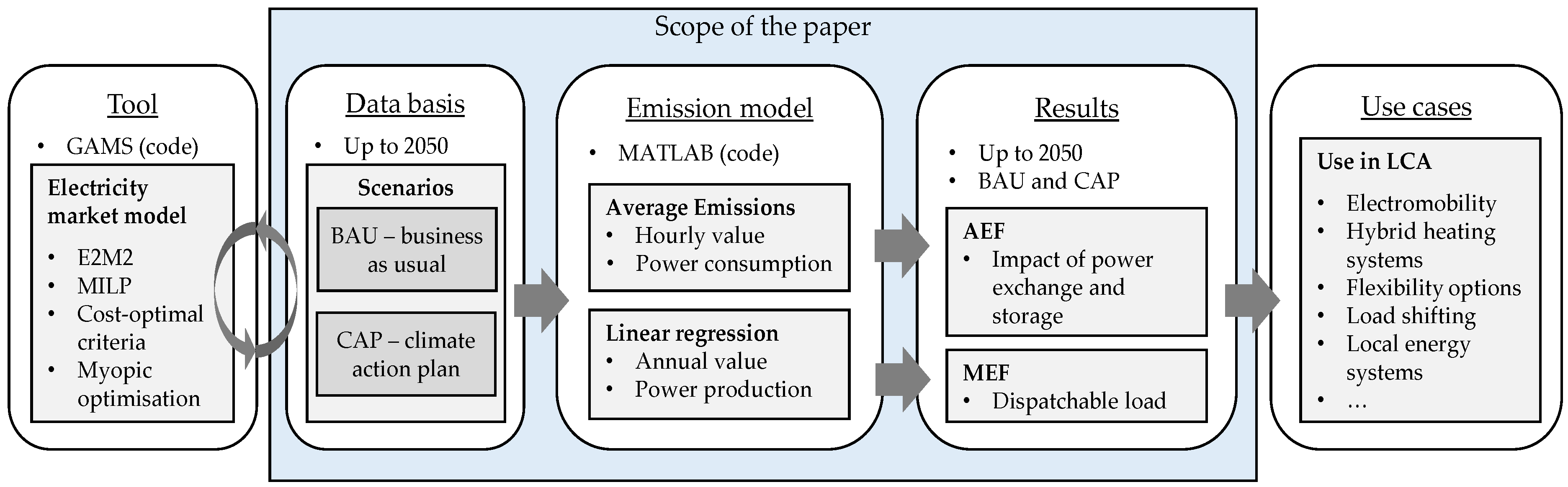
In a first step, the two power supply scenarios are calculated in an electricity market model. Figure 1 shows the individual process stages with the respective software used and the respective interfaces (arrows). The data basis and the emission model for the determination of the hourly factors are described mathematically in Section 2. The scope of the paper includes the developed scenarios, the emissions model, the presentation, and discussion of the results.
2.1. Data Basis: The Electricity Market Model E2M2
The data of hourly emission factors up to 2050 are based on scenarios of the power production that were developed in the course of the Kopernikus project ENavi (Energiewende-Navigationssystem) and were strongly adapted for this paper. The Institute for Energy Economics and Rational Use of Energy (IER, Stuttgart, Germany) at the University of Stuttgart worked on this research project and used the European Electricity Market Model (E2M2) developed at the IER [54]. The E2M2 is a mixed-integer optimization model that models the competitive electricity market, thereby determining investment decisions and the dispatch of power plants endogenously under cost-optimal criteria [55].
As input parameters, the existing power plant park including fluctuating renewable energies, storage facilities, potentials for renewable energies (e.g., wind offshore), electricity demand, political objectives, investment costs, technological and other economic parameters, and flexibility options are taken into account. The electricity reduction method (power loss factor) is used to allocate the fuel quantities for combined heat and power plants, which is an important detail for the determination of emission factors [24]. The total amount of the electricity trade balance is specified in the model as an annual sum for each scenario and then distributed model-endogenously for each hour. This means that in one year, either imports or exports are possible. Limitations of electricity transmission within Germany were not considered—but limitations of transmission with surrounding countries were considered. Thus, the model determines the hourly power plant operation in Germany in a myopic optimization for eight milestone-years from 2015, 2020 … to 2050. The detailed configuration of the input parameters and the modeling process itself are not part of the research in this paper. A more detailed model description can be found in [55,56,57,58].
2.2. Utilised Scenarios
The scenarios do not constitute forecasts, but rather possible alternative developments based on the current power plant park (brownfield scenario). Scenarios help to understand these developments in complex systems such as energy supply [56]. The reproduction of a functioning electricity market is the decisive point for the formation of prospective hourly emission factors. In this way, the temporal dynamics of the emission factors, from hourly fluctuations to long-term annual changes, can be taken into account. The scenario results described in the following should therefore only be seen as two possible trends to demonstrate the application of the methodology.
The construction and decommissioning of power plants, which have already been decided upon, have been modeled unit by unit. For this paper, the German coal and nuclear power phase-out was implemented with specific phase-out dates in accordance with the regulatory requirements [59]. Since the date of phase-out for hard coal-fired plants will be determined in an auctioning process, the order of shut-down is not yet known. Therefore, it is assumed that hard coal-fired power plants are taken off the grid in an orderly manner after the year of commissioning. This way, the oldest hard coal-fired power plants are always taken off the grid one after the other in a linear ideal-typical decommissioning path. This assumption can differ from actually being correct, as can be seen from the decommissioning of the quite new Moorburg power plant.
In the Business-As-Usual (BAU) baseline scenario, emissions from power production are reduced by 74% in 2050 compared to 1990, and the share of renewables in net power production (NPP) increases to 57% (2030:43%).
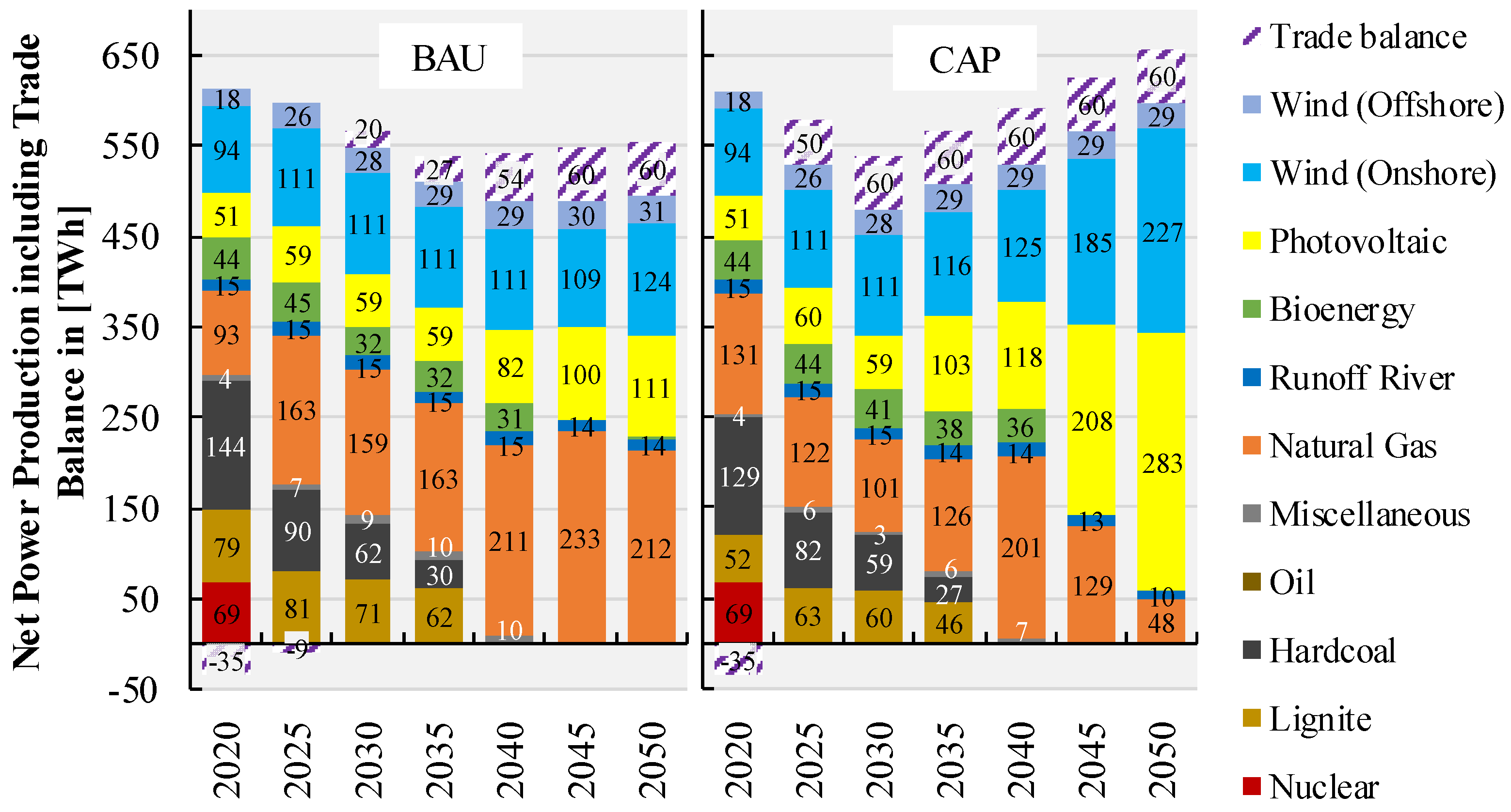
In the Climate-Action-Plan (CAP) scenario, the emissions cap for the energy industry is adjusted in line with the total emission reduction of the German climate action plan (as shown in Figure 2). This means that GHG emissions from power production will be reduced by 95% in 2050 compared to the base year 1990. The share of renewables in NPP is 92% (2030:50%). The development of demand and the maximum power exchange balance of the two scenarios was based on the scenarios of the study “Klimapfade für Deutschland” [60]. In the scenarios, Germany develops from a net power exporting country to a power importing country with a maximum power exchange balance of 60 TWh per year. This external model parameter limits the annual power exchange balance to the highest value that has occurred in Germany in the last 30 years. The assumption of a higher demand in the CAP scenario is driven by more electrification measures in heat supply and transportation sectors. This means that two scenarios are formed as a data basis, which show a different but possible development of power production in Germany and enable an illustration of the method that has been applied and developed. The results of the optimization model are shown in Figure 3 and Figure 4.
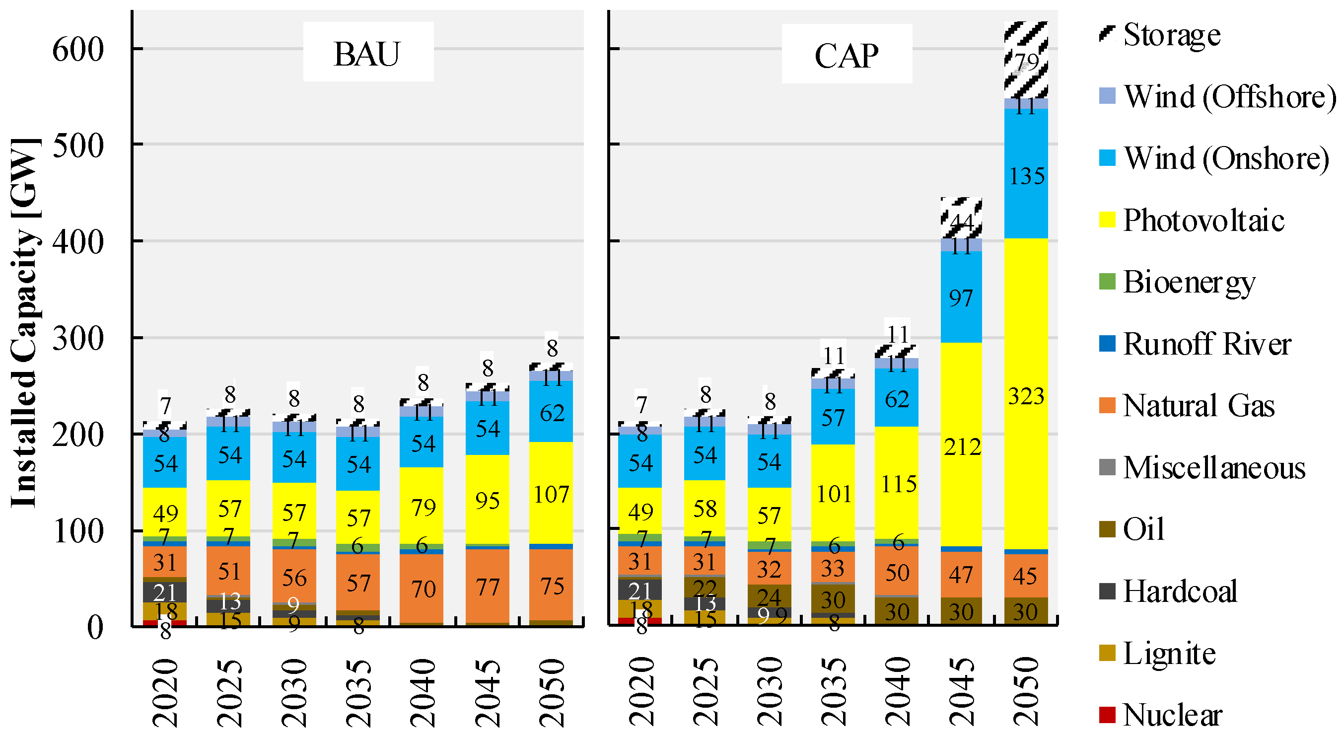
In addition to the phasing out of nuclear energy and coal, a continuous increase in NPP from renewable energies can be seen. In the BAU scenario, the GHG emission cap is still at a level that allows for the massive expansion of gas-fired power plants. In the CAP scenario, this expansion must be increasingly replaced by electricity from photovoltaic and wind power plants, which is accompanied by a massive expansion of the installed capacity of renewables and storage facilities and cheap backup capacity with oil-fired power plants. Additionally, the expansion of renewables leads to very high quantities of curtailed electricity (curtailment BAU 2050:16.3 TWh; CAP 2050:123.9 TWh). The lack of power from bioenergy in 2045 and 2050 is due to an increased price for biogenic fuels, driven by the competing use of the relatively low potentials in the industrial and mobility sector. From the beginning of the optimization in 2015 with 7.68 €/t to 18 €/t in 2020, the price for CO2 (EU allowances) increases continuously to 150 €/t in 2050. These assumptions apply to both scenarios.
2.3. Calculation of the Developed Emission Factors
2.3.1. Fuel-Specific Emission Factors
To comply with the GHG emission cap in the electricity market model, only GHG emissions from direct combustion without upstream emissions from the German power production were used. This corresponds to the UNFCCC calculation guideline for the determination of GHG emissions from power production, which was used as the underlying basis for the development of the scenarios. The electricity market model also takes into account the efficiency of the various fossil power plants and their start-up and shut-down behavior. Therefore, an emission factor for the amount of electricity generated cannot be given, but more precisely, a factor for the thermal energy released by the fossil fuel can be given (as shown in Table 1). The fuel-specific factors are taken from the mandatory National Inventory Report for Germany [61].

Table 1.
Emission factors used for the different energy sources.
| gCO2eq/kWhth (Efec) | gCO2eq/kWhel (Efre) | ||||
|---|---|---|---|---|---|
| Type of Energy Source 3 | Fuel Combustion 1 | Upstream 2 | LCA-Ef | LCA-Ef | |
| Natural Gas | 204.4 | 33.1 | 237.5 | - | |
| Hardcoal | 338.2 | 50.5 | 388.7 | - | |
| Lignite | 404.4 | 9.3 | 413.7 | - | |
| Miscellaneous 4 | 270.3 | 20.2 | 290.5 | - | |
| Oil | 282.6 | 12.3 | 294.9 | - | |
| Nuclear | 13 | ||||
| Bioenergy | - | - | - | 41 | |
| Photovoltaic | 46.8 | ||||
| Runoff River | 6.6 | ||||
| Wind | Offshore | 11.4 | |||
| Onshore | 11.1 | ||||
1 Lower heating value, with climate carbon feedback and GWP100 for methane and nitrous oxide [1]. 2 The entire life cycle, including transport and material input up to the provision of the energy sources without disposal and incineration according to the Global Emission Model of Integrated Systems—GEMIS [62]. 3 Weighted averages from the German mining regions [61,63] and the median of the meta-analysis of the National Renewable Energy Laboratory [64] {XE “NREL”\t “National Renewable Energy Laboratory”}. 4 Landfill gas, sewage gas, municipal waste, wood residues, and biomass [61].
2.3.2. Average Emission Factor
The fuel input of fossil and renewable sources resulting from the generating units and their efficiency of power production is multiplied by the respective specific emission factor of the fuel (Equation (1)). Specific emission factors related to the power generated from RES and nuclear energy are used to calculate the emissions of RES. This results in the total hourly GHG emissions of gross power production in one milestone-year .
In the case of exports, the trading balance is assessed with the hourly emission factor of net power production shown in Equation (2), and the resulting GHG emissions are deducted from total GHG emissions (Equation (4)), with as the net power production in hour and milestone-year .
Following [16], which calculates an electricity mix factor from data of the European Network of Transmission System Operators for Electricity (ENTSO-E, Brussels, Belgium), the European emission factor is used for the assessment of electricity imports (Equation (4)). The IEA provides daily load profiles of electricity demand and average emission factors of the European Union in hourly resolution. In a “Stated Policies” and a “Sustainable Development Scenario”, possible future developments up to the year 2040 are modeled and continued on a linear basis until 2050 [65]. The grid losses associated with hourly net power consumption are calculated on the basis of the current German grid losses for 2018 at 4% of gross power production, comparable with [36,66].
For an emission factor of power consumption, the energy for electricity storage is first not assigned to final energy consumption. The energy from discharging pumped storage and battery storage facilities is already burdened with GHG emissions when the storage facilities are charged. The energy from the discharging process is therefore compulsorily regarded as emission-free and reduces the emission factor in the hour concerned. At the time of charging, the electricity required for this purpose is consequently not made available in the power grid, the emission factor will therefore become higher at this time and a temporal distortion will occur when emission factors are considered on an hourly basis [35,67]. Traceability of emissions is impossible due to intermittent charging and discharging processes, as well as variations in storage duration and the non-traceability of charge carriers (electrons). In order to minimize these distortions and to better reflect the emission factor of net power consumption, a specific emission factor for electricity storage, based on [67], is calculated endogenously.
First, the virtual emissions of the charging process, thus the required charging power, are calculated. For this purpose, the hourly emission factor of the net power production is multiplied by the power demand of the storage facilities’ charging process (storage in) at hour . The annual sum of the virtual emissions is divided by the annual sum of the electricity quantity from storage (storage out). This results in an annual emission factor for the electricity produced from storage facilities, based on the average emissions emerged during the storage period (Equation (3)). The lower the emission factor for charging, the lower the emissions of the electricity provided from the discharging process. It is assumed that imported and discharged electricity is not used for charging.
As shown in Equation (4), the total GHG emissions of gross power production at hour , minus exported GHG emissions and those from charging, plus imported GHG emissions and emissions of the amount of electricity discharged, are divided by the total net power consumption . This creates the hourly average emission factor of net power consumption . Depending on which fuel-specific emission factors are used, the AEF is referred to as AEFfc for fuel combustion or AEFlca for life cycle assessment.
2.3.3. Marginal Emission Factor
The direct (short-term) MEF presented in this paper is calculated according to [30] using the linear regression method from the amount of net power production provided by dispatchable () and fossil-fueled power plants and the resulting emissions between two consecutive hours and (Equation (5)). The gradient of the regression line from over represents the yearly average MEF. The regression line is derived from 8760 hourly values for each milestone-year. The authors of [49] demonstrate that a more detailed temporal granularity for Germany is associated with an increasing deterioration of the coefficient of determination.
The MEF is intended to reflect the change in emissions through an active change in demand within Germany. Renewables such as wind power and photovoltaics will not take on this active role due to the functioning of the German electricity market and the feed-in priority of RES [35,36,39]. Thus, the MEF does not take into account renewable energy production, storage, and trading volumes. Storage technologies can only provide a limited amount of power under certain conditions. Although electricity trading volumes can be considered a hypothetical marginal “power plant” [39], they are not included in this analysis. Theoretically dispatchable power plants include thermal power plants burning fossil fuels and nuclear power plants. Similar to the AEF, the MEF is referred to as MEFfc for fuel combustion or MEFlca for life cycle assessment.
3. Results
3.1. Analysis of the Average Emission Factor
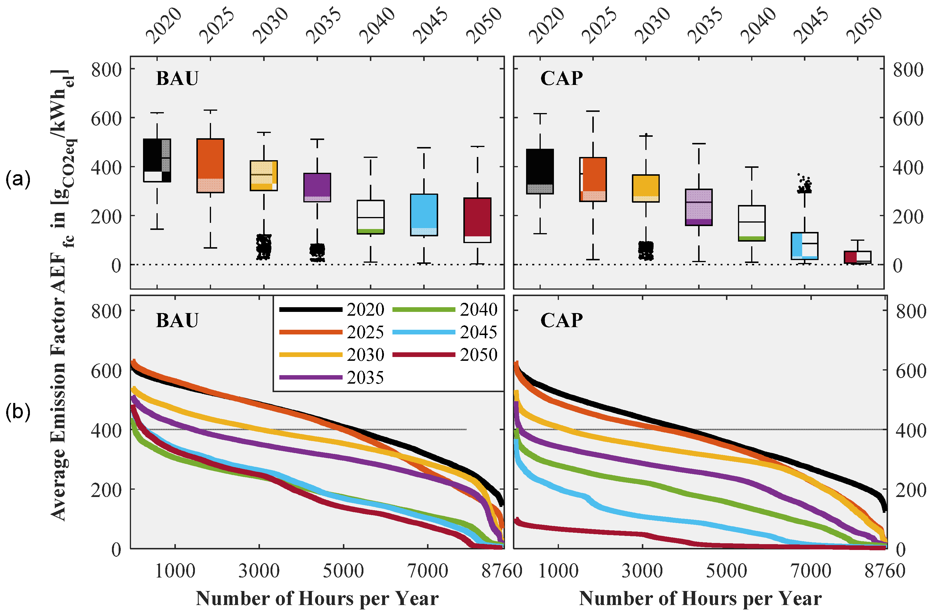
The duration curves for the two scenarios shown in Figure 5 illustrate the wide range of the developed AEFs. The median of the annual AEFfc decreases continuously due to the forced phase-out of coal combustion in both scenarios. The coal phase-out is clearly shown by a jump in the duration curves from 2035 onwards. Merely in the BAU scenario, the AEFfc decreases only insignificantly from 2040 on. Caused by the phase-out of bioenergy, despite meeting the emissions cap, the median even rises slightly to 2045. The spread of the values and also the peak AEFfc remain constantly at a high level and only reach lower values in 2050 in the scenario CAP, where the highest AEFfc is then 100 gCO2eq/kWhel. The AEFfc can drop much further in CAP and reach almost 0 gCO2eq/kWhel, because the expansion of RES and electricity storage massively increases. Due to the applied calculation method of GHG emissions from electricity storage and must-run restrictions, reaching exactly 0 gCO2eq/kWhel in these scenarios is almost impossible. Furthermore, for imports from the EU for the years 2045 and 2050, in some hours the power is already being produced exclusively emission-free. Overall, in 2050, CAP in 3709 h and BAU in 660 h will fall below 10 gCO2eq/kWhel.
With a GHG reduction of 74% in BAU, the average annual AEFfc by 2050 falls only slightly to 183 gCO2eq/kWhel. While the other duration curves show a clear reduction of the emission factors in the peak values from year to year, those of 2025 in the BAU scenario are initially higher than the present-day peak values. This fact has to be credited to the phase-out of nuclear energy and its substitution by increased power production from lignite-and gas-fired power plants. The situation is similar in the years 2045 and 2050 with the decreasing amount of bioenergy. The peak values of the AEFfc when no renewables are fed into the grid result from the adjustment with gas-fired power plants, whereas in 2040, bioenergy could still contribute a part to that.
When calculating the AEFlca with the corresponding LCA-Ef (as shown in Table 1), a similar course of the duration curves and distribution of the values can be seen. However, the average annual AEFlca in all milestone-years is between 30 and 60 gCO2eq/kWhel higher than the AEFfc. Because of the continuously decreasing AEF until 2050, the average annual AEFlca in 2020 is still less than 10% higher than the AEFfc, while in 2050 it is twice as high in the CAP scenario.
3.1.1. Distribution within the Year
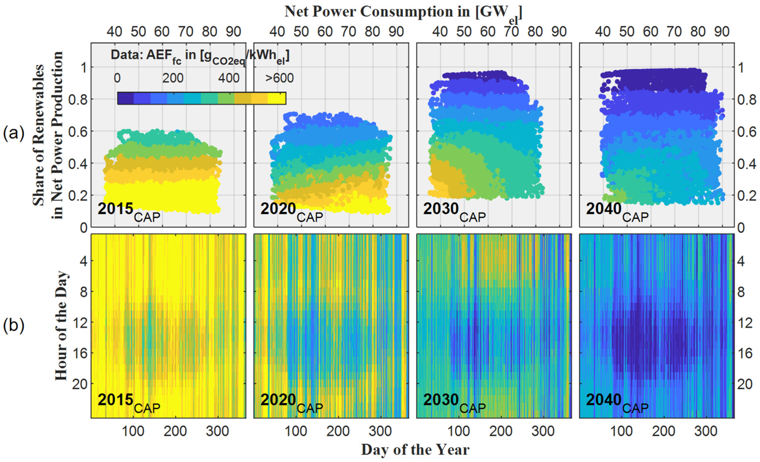
Figure 6 shows the AEFfc for 2015, 2020, 2030, and 2040 in the CAP scenario in a heat map (b) and as a scatterplot (a) with the hourly values’ relation to net power consumption and the share of RES. The data from 2015 are shown for comparison, as a backtesting of the model was carried out here with respect to the electricity production volumes and installed capacities. The area with low AEFfc values is clearly visible due to the influence of photovoltaics and wind energy during the increased solar radiation at midday and in early summer to autumn. In addition, periods of increased wind power input over several hours can be seen as a vertical strip.
3.1.2. Intraday Distribution
When looking at the intraday fluctuations of the AEFfc,lca, it can be seen that in 2020 the highest values still occur in the morning between hours 6 and 8 and in the evening hours between hours 21 and 23. This peak value shifts in later years to the earlier morning between hours 3 and 6 and weakens in the evening hours. Due to the feed-in from photovoltaics, typically the lowest values are at midday in all scenarios and years. That photovoltaic sink is less visible in the CAP scenario from the year 2045 on and is no longer visible in 2050 with the LCA-Ef.
3.1.3. Load and Renewables Feed-in
The share of RES in net power production in 2020 varies between 8.5% und 70.7% (as shown in Figure 6). The AEFfc and the share of RES are negatively correlated (). While the share of RES and the distribution of AEFfc values occur in almost all load ranges, it can be seen that in 2020, higher AEFfc of more than 400 gCO2eq/kWhel will occur more frequently, even at higher loads. This effect is reversed in 2030 and 2040—with increasing demand, the AEFfc decreases. The integration and expansion of RES will make it easier to cover peak load periods, although in 2030 the absolute peak load (>80 GWel) will not yet show values below 200 gCO2eq/kWhel. In addition, in 2030, fossil-fueled power plants still in existence will be running at base and medium load, which will greatly increase the AEFfc when demand is low. For the year 2040, this effect can also be explained by the simultaneity of little wind and photovoltaic feed-in and the low demand between Christmas and New Year.
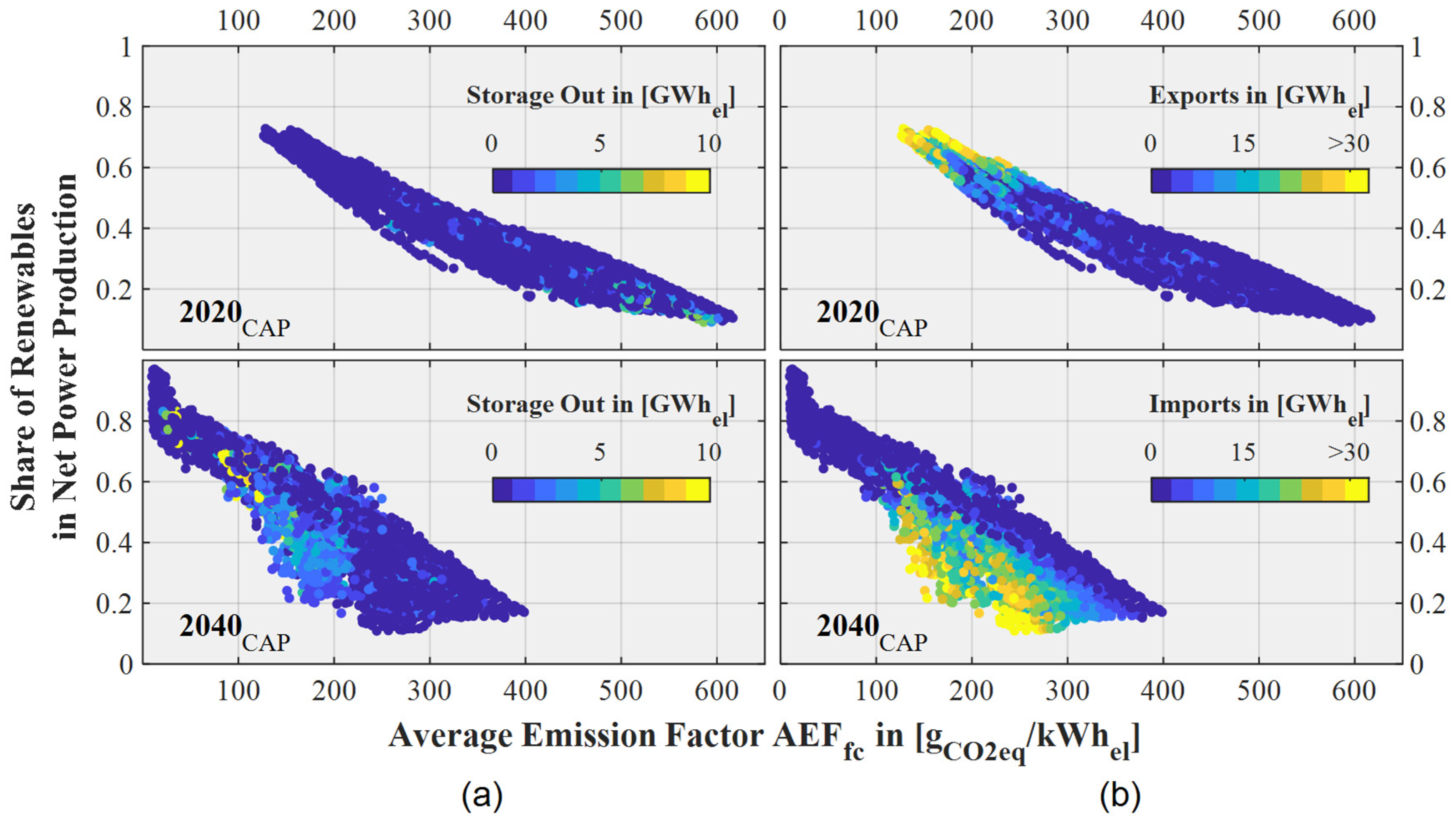
Figure 7 shows the connection between the RES feed-in and the AEFfc. The shift of the data cloud from 2020 towards lower values (to the left) in 2040 shows the influence of the coal phase-out. The scattering of data points without significant trading or storage impacts at the same share of renewables can be explained by the different composition of the residual load in terms of power plant efficiency and energy carriers. The largest export volumes in 2020 will appear when there are high shares of RES in the power supply (as shown in Figure 7b). Export power is assessed with the emission factor of net power production, which means that exports do not significantly affect the hourly specific AEFfc, because the two emission factors have similar values. However, the absolute emission level of power production is still influenced by the export of mainly RES electricity.
In 2040, AEFfc of less than 300 gCO2eq/kWhel will be apparent, despite low RES shares of less than 20%. Although gas-fired power plants meet the majority of demand here, the fairly low-emission imported electricity and the lower-emission electricity from storage facilities reduces the AEFfc in these times (Figure 7a). Here, the emission factor of imported electricity is significantly different from the emission factor of net power production. Due to higher demand in 2040 than in 2030, with the installed capacity of fossil power plants remaining unchanged, it is possible that, despite the ongoing expansion of renewables and a reduction in GHG emissions, lower shares of renewables in NPP may still occur in some cases (as shown in Figure 6). The BAU scenario tends to show the same effects with overall higher factors.
3.2. Analysis of the Marginal Emission Factor
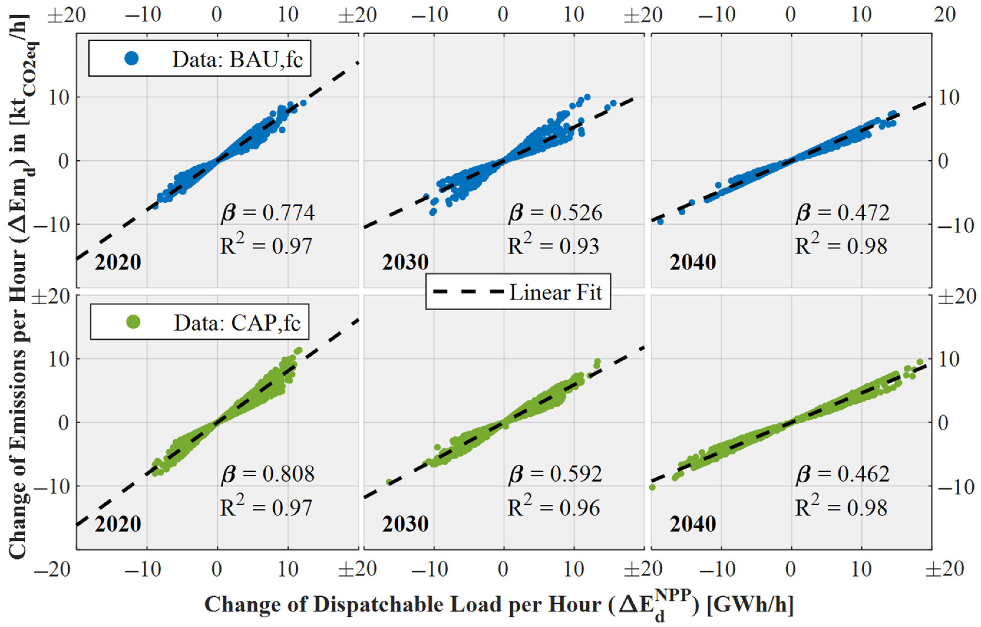
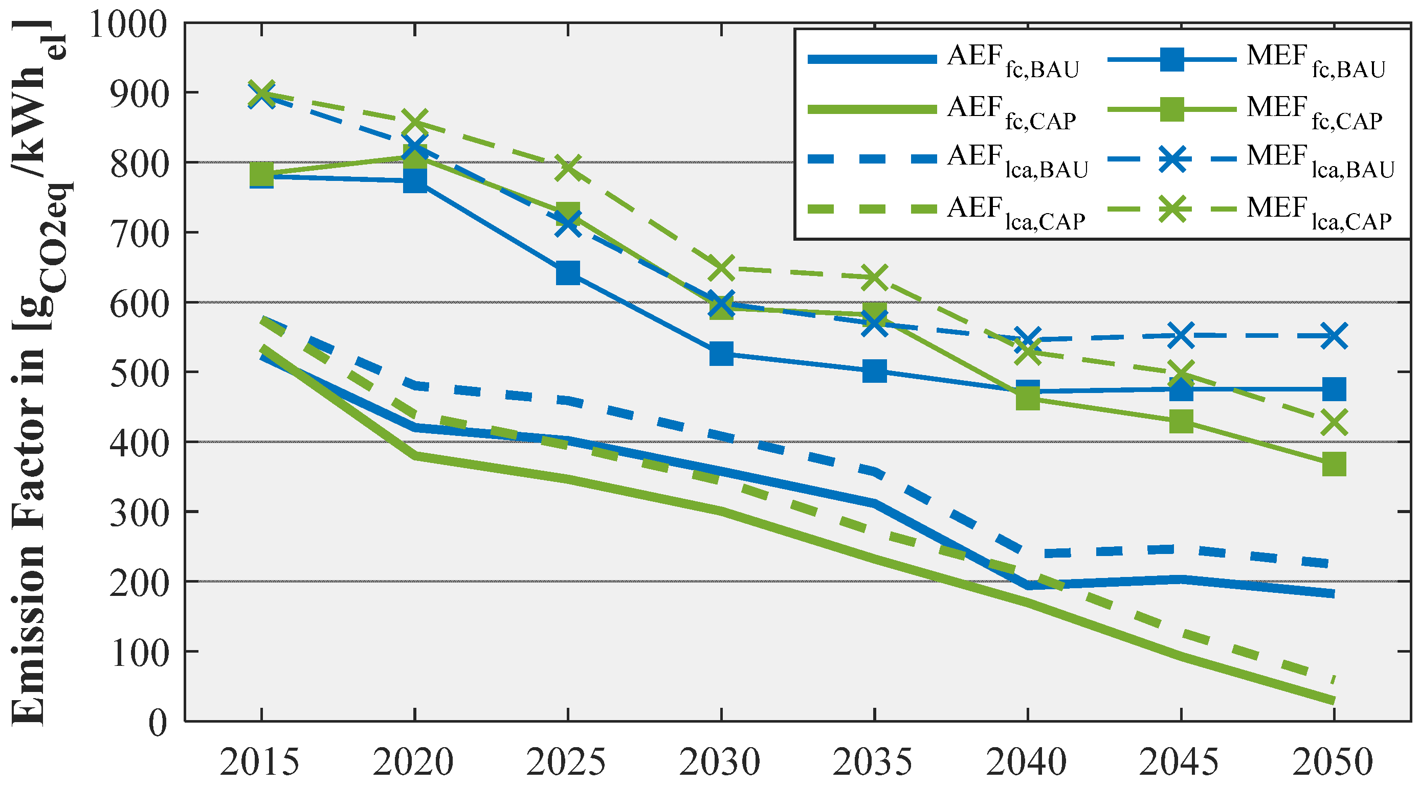
The average MEFfc in 2020 is over 770 gCO2eq/kWhel in both scenarios. These are the GHG emissions that an additional demand increase by one kilowatt-hour in 2020 causes on average. It is assumed that the demand change will only be met by domestic, conventional, dispatchable power plants. Figure 8 shows the hourly values of the change in load and the corresponding change in emissions . The gradient of the linear regression line represents the average annual MEFfc. The coefficient of determination is above 0.93 in all milestone-years.
In 2020, the MEFfc is still strongly influenced by coal-fired power plants, which play a significant role in load changes. The higher value in the lower-emissions scenario CAP is due to the fact that here, more gas-fired power plants also provide base load and coal-fired power plants react to load changes more often than in the BAU scenario and provide less base load. In other words, although the entire generation is lower-emission, the more emission-intensive power plants also react to changes in demand and peak load. The capacity factor (Cf) of the group of gas-fired power plants is 34.5% in the BAU scenario (CfCoal,2020: 77.2%; CfLignite,2020: 49.6%) and 48.4% in the CAP scenario (CfCoal,2020: 69.0%; CfLignite,2020: 33.1%).
Furthermore, it can be seen that the data points spread out slightly from the zero crossing. The load changes are characterized by different emission-intensive power plants and the data cloud indicates a line of coal and a line of gas power plants comparable to [27].
The same effect of spreading out around the linear fit caused by the different shares in the change in demand of the different power plant classes can also be observed in 2030, especially in the BAU scenario. The higher MEFfc of the CAP scenario is also caused here by the gas-fired power plants running in more base load compared to the BAU scenario. The Cf of the gas-fired power plants in the BAU scenario is 32.3% (CfCoal,2030: 80.3%; CfLignite,2030: 86.6%) and in the CAP scenario 35.8% (CfCoal,2030: 76.7%; CfLignite,2030: 73.4%).
In 2040, only natural gas and, in very small quantities, oil will be combusted for fossil, dispatchable power production. This means that, with a similar use and efficiency of the power plants, the MEFfc of the scenarios becomes more or less the same.
Despite the fact that in both scenarios, almost exclusively gas-fired power plants act as marginal power plants, the MEFfc in the CAP scenario falls to 368 gCO2eq/kWhel by 2050 and is thus significantly lower than the MEFfc of 475 gCO2eq/kWhel in the BAU scenario. This discrepancy is due to the fact that in the CAP scenario, considerably less installed capacity and energy quantities of gas-fired power plants are used and thus relatively more combined-cycle gas turbine power plants with combined heat and power generation are used to react to changes in load than the more inefficient open cycle gas turbine power plants. The annual average net efficiency of the aggregated gas-fired power plants in 2050 is 45.4% for the BAU scenario and 54.7% for CAP.
3.3. Summary of the Evaluated Emission Factors
The average annual emission factors shown in Figure 9 still show the origin of the scenarios in 2015 with, depending on the characteristics and type of emission factor, identical starting conditions in both scenarios. The level of the emission factors differs greatly from the type, AEF or MEF, and additionally in the selection of the fuel- or energy source-specific emission factors with regard to the life cycle perspective. Table 2 shows the corresponding values and associated standard deviation of the hourly values. The hourly values of both scenarios are made available in the Supplementary Materials.
4. Discussion
4.1. Application and Use of Emission Factors
On the basis of the two current scenarios for the development of power production, the timely course of the planned power plant decommissioning and the German government’s objectives for the expansion of RES and the reduction of GHG emissions can be depicted with varying intensity. Thus, it is possible to use the emission factors generated in life cycle inventories, which correspond to a conservative, slower transformation of energy systems and a faster, lower-emissions power production by 2050. From this, different implementation dates for electrification measures or also implementation dates for a bivalent use of energy sources and flexibility options can be determined.
The heat maps in Figure 6 show the effects of the underlying average weather year used. The fluctuating renewable energies depend on the meteorological conditions and influence the AEF directly on the basis of this profile.
The EU-Joint Research Centre (JRC, Brussels, Belgium) differentiates the application of life cycle assessments into four types, also called situations. According to the International Reference Life Cycle Data System (ILCD-standards) [68], the calculated direct MEF is counted to situation A, with which decisions on changes in demand, for example through the implementation of electrification measures, can be assessed. In situation A, the effects of the decision are so incremental that, regardless of which choice is made, no structural changes, such as a resulting new construction of power plants, occur. The developed AEF can be counted to Situation C. If the purpose of the LCA is solely descriptive and does not lead to structural decisions and changes, then situation C is applied.
4.2. Importance of Hourly Emission Factors
Röder et al. applying constant and dynamic emission factors (AEFfc) in today’s and future sector-coupled urban energy systems [19]. They come to the conclusion that the wider the distribution of the emission factor, the bigger is the impact whether a constant instead of a time-resolved emission factor is used [19]. Figure 5 shows that the range of the values is constantly over 400 gCO2eq/kWhel in all years, except for the year 2050 in the CAP scenario, thus again emphasizing the advantages of the hourly dynamic emission factors for ecological assessment methods.
4.3. Improvement of the Calculation Method
The methodological enhancement allows the correct allocation of emissions from electricity exchange between different regions and storage at the time of the actual use of electricity. By using an endogenously determined emission factor for export volumes and discharging processes, taking into account grid losses, auxiliary consumption, and imported emissions from the EU, the actual emission factor of power consumption, and not that of power production, can be determined. This will allow a more accurate calculation of the emissions from electrification measures and life cycle assessments of electric applications, which usually use the electricity from the public power grid at the very end of the transmission chain. Furthermore, the prospective scenarios can also take into account the change in the system of power generation and thus calculate lifetime emissions for the use of electricity-based applications.
4.4. Comparison with Other Research
The results of the relevant publications described hereafter are presented comparatively in Table 3. The fuel-specific emission factors used in [18] are derived from ecoinvent’s LCI, taking into account life cycle emissions and assessing the amount of electricity produced, whereas in this paper, the used fuel-specific emission factors were determined for the combustion of fossil fuels prior to their conversion in thermal power plants. This way, different efficiencies and a partial load operation of the power plants could be considered. Similar to [18], the effect could be observed that lower AEFs occurring at times of increased photovoltaic feed-in and also at weekends at lower load (Figure 6a). However, the more prospective consideration here shows that the load-dependent effect is reversing further in the future.
The AEFfc calculated by [50] is higher in both comparable scenarios. The calculation is based on several energy scenarios with information on the installed capacity of the generation units in the future power plant park. The average annual CO2 emissions from power production are determined using the capacity factor and a power plant-specific emission factor. The authors consider different values of fuel-specific emission factors using a Monte Carlo simulation. The available emission factors of this research work were formed on the basis of the National Inventory Report for Germany, taking into account regional and technological specifications (Table 1). Furthermore, the hourly values with different power plant efficiencies (partial load behavior) and the data basis of an hourly optimization model of the German electricity market are not necessarily comparable with the annual calculations of [50].
In [51], hourly emission factors of power production were calculated using three type days per season in an energy system model. The time horizon extends to the year 2030 with the aim of determining different charging times based on the emission intensity of the electricity used at the same time. No trading effects were considered, and specific emission factors per generation class (coal, lignite, …) were applied. To determine the indirect MEF, a specific load profile derived from the charging cycles of battery electric vehicles is added to the conventional load in the optimization model. From this, an emission difference due to a changed dispatch and newly built power plants was calculated. Hence, the indirect MEF here is only valid for that particular load change and cannot essentially be compared to a more general MEF.
The exploratory scenario used by [35] for the generated hourly prospective emission factors is most comparable to the CAP scenario. However, the exploratory type is recommended for modeling indirect MEF [7]. In the normative scenarios presented here, the linear optimization model determined the expansion of power plant capacity endogenously for each unit by meeting the CO2 caps. Consistent with a trend scenario, the increase in demand in [35] until 2050 is lower than in the CAP scenario shown here. Furthermore, there is a stronger expansion of wind power plants and a lower expansion of photovoltaic plants, but a similar development in the capacity of gas-fired power plants. The lower values of the AEFfc (except 2050) are mainly explained by a much faster expansion of RES and the allocation method used (Carnot method). In [35], all emissions generated were directly allocated to the simultaneous demand for electricity, so the emission factor of discharged power automatically corresponds to that of the simultaneously reduced generation capacity. Basically, the same assumptions and methods were used to account for trading and its emissions. The main difference is that in this research work, the emission factor of the neighboring countries from which the power is imported is aggregated as an exogenous model parameter at a European level. Due to a completely different choice of methods, even lower MEFs than those of this research work may occur there.
4.5. Share of Renewable Energies as an Indicator for the AEF
The authors of [52] demonstrated that RES can be used as an indicator with a similarly high coefficient of determination for the AEF. However, the shift due to trading effects, pumped storage, and the assessment of the net power consumption showed that a deeper analysis is needed to determine the actual AEF of a particular hour (Figure 7). The share of RES in the NPP should therefore not be used as an indicator of the emission intensity of the electricity used.
4.6. Critical Review of the Emission Factors
A general point of criticism of the development of prospective emission factors is the quality of the data basis and the underlying assumptions of the scenarios and the development of the future power supply. The focus here is not necessarily on the influence of a possible earlier coal phase-out, a different expansion of renewable energies, or the development of energy carrier prices, but rather on changes in energy-specific laws, assumptions on dispatch rules, grid restrictions, exchanged trading volumes, and storage management. The authors are thus aware that future emission factors can and will develop differently due to the actual evolution of power supply in Germany and Europe. Therefore, the focus of the analysis was on the calculation method for hourly prospective emission factors and the consideration of trading and storage effects. The scenarios used can always be updated and improved. This only changes the data basis, and the calculation model can still be applied.
An inaccuracy in the calculation method is the exclusive consideration of the trade balance. Due to the export of virtual emissions and the import of relatively low-emission power from other European countries, the emission factor could reach even slightly lower values. To generate trading volumes between different countries in hourly resolution as endogenous model parameters requires very sophisticated energy system models with long calculation durations and is therefore not met in full detail in any publication known to the authors for prospective emission factors.
Another possible inaccuracy is the determination of virtual emissions of the charged power. The created discharge factor is an annual average of the virtual stored emissions. This is necessary, because otherwise it would not be possible to assign an emission value to the power usage at the corresponding hour. Average storage durations and intervals could perhaps be used as an indicator and the annual discharge factor could be differentiated more precisely.
The MEF is strongly influenced by the assumptions made on the dispatch of the power plants. In the future power generation system in Germany, bioenergy could become a marginal power plant. The Renewable Energy Sources Act-tariff ensures that a high capacity factor of renewable energy plants is most economical. This is also probably the most likely way to reduce GHG emissions at the present time. That is why bioenergy power plants in Germany are still inflexible, even though there is a flexibility bonus. Because of the increased need for flexibility due to a decrease and negative residual load and the integration of renewables, the currently typical dispatch of power plants could be changing. A marginal change in demand can be compensated by the availability of a flexibility option rather than by an adjustment in load by conventional power plants. Furthermore, the method shown does not take into account the occurrence of non-grid related excess power but could be subject to future research.
5. Conclusions
The main results of this paper are the generated prospective hourly AEF and annual MEF. In order to improve the adequate ecological assessment of electrification measures over their lifetime, the emission factors were calculated from two scenarios with different degrees of decarbonization up to the year 2050. This was accomplished by utilizing an electricity market model (optimization model) based on CO2 caps and by creating brownfield scenarios with possible future developments. From this data basis, the effects of electricity trading and the storage facilities could be integrated into the AEF using the emissions model. In combination with the grid losses, the GHG emissions were correctly applied to the power consumption. This has the consequence that imported and exported power is given an emissions intensity and thus the impact of an electricity import can also be credited in proportion to the final consumer of the electricity. The discharged power from storage facilities is assigned an emission intensity depending on the emission intensity of the stored power. Thus, the hourly AEF is significantly less distorted by the discharged power. The emission factors can also be used to demonstrate the influence of the German coal phase-out implemented in the scenarios. The additional use of upstream emission factors for the energy sources used in power production show that the influence of upstream emissions plays an increasing role in a strongly decarbonized power production system. The hourly emission factors have been made available for open-access use in life cycle inventories.
The AEF generated takes into account, through the calculation method, effects from electricity trading, GHG emissions caused and delayed by electricity storage, the varying efficiency of the power plants, and varying specific emissions from the power generation of individual power plants (partial load behavior) caused by constraints on the electricity market. Although the AEF falls substantially in all scenarios, the value remains constant in the BAU scenario (−74% GHG emissions) in the later years at a level just below 200 gCO2eq/kWhel and can only fall significantly further in the CAP scenario after 2040. A significant number of hours per year of almost emission-free power only occurs in the CAP scenario in the latter years.
The generally higher MEF, compared to the AEF, will decrease with the phasing out of coal-fired power generation but will not fall below 368 gCO2eq/kWhel. An important finding is the initially higher MEF of the CAP scenario, while more CO2 is reduced overall. Gas-fired power plants are increasingly used to provide base load, and coal-fired power plants have to respond more flexibly. This is the only way to meet the stricter CO2 cap, although the MEF is higher.
The exchange of power, mainly imported power, with the rest of Europe has a significant impact on the AEF. Together with the lower-emission electricity from the discharge of storage facilities, the AEF is also significantly reduced, and this is despite a small share of RES in net power production.
With the high temporal resolution of dynamic factors, flexibility options, sector coupling technologies, and specific decarbonization measures, such as power-to-gas and power-to-heat, can be analyzed with regard to their GHG reduction effects. With these technology options it is decisive determining when lower-emission power can be used to replace fossil energy carriers. With the hourly prospective AEF for Germany, for example, the effects of the electrification of industrial process heat on greenhouse gas emissions can be calculated. The few annual averages used so far, as in Schüwer and Schneider [69], do not make it possible to determine the deployment strategy and GHG emissions of hybrid heat generation technologies. In addition, the dynamic charging profiles of battery electric vehicles, as in Axsen et al. [45], or time-of-day specific energy efficiency measures, as in Bettle et al. [32], can be assessed with concrete GHG emissions from using grid electricity.
Further research is needed regarding the necessity of hourly-resolved MEFs, the investigation of changing dispatch behavior in the German and European electricity market, and the integration of a more detailed view of trading and storage effects as well as the increasingly frequent occurrence of curtailed excess power in future power supply systems with large volumes of fluctuating renewable power. The more precise representation of trading volumes in the future electricity market can make the AEF even more precise. Future research could combine a marginal emission factor for power trading with the method of linear regression, as in [39].
Supplementary Materials
The AEFfc and AEFlca for both scenarios are available online at https://osf.io/9v6bx/?view_only=edfea9ab1fec4f23a583958802986c85.
Author Contributions
Conceptualization, review, methodology, simulation and visualization of the emission model, data curation, writing, editing—all sections: N.S.; editing, supervision, and conceptualization: P.R. All authors have read and agreed to the published version of the manuscript.
Funding
This research work was made possible by a scholarship from the Graduate and Research School for Efficient Energy Use Stuttgart—GREES. The authors are solely responsible for the content of the research work.
Institutional Review Board Statement
Not applicable.
Informed Consent Statement
Not applicable.
Data Availability Statement
The data presented in this study are openly available in [https://osf.io/9v6bx/?view_only=edfea9ab1fec4f23a583958802986c85] at [doi:10.17605/OSF.IO/9V6BX].
Acknowledgments
Many thanks go to Annika Gillich for her kind support and assistance with the scenarios created in E2M2 which made this paper possible.
Conflicts of Interest
The authors declare no conflict of interest.
References
- Intergovernmental Panel on Climate Change (IPCC). Climate Change in 2013: The Physical Science Basis; Working Group I Contribution to the Fifth Assessment Report of the Intergovernmental Panel on Climate Change; IPCC: Cambridge, UK; New York, NY, USA, 2013. [Google Scholar]
- Bundesministerium für Umwelt, Naturschutz, Bau und Reaktorsicherheit (BMUB). Klimaschutzplan 2050. Klimaschutzpolitische Grundsätze und Ziele der Bundesregierung; BMUB: Berlin, Germany, 2016. [Google Scholar]
- International Energy Agency (IEA). Global CO2 emissions in 2019, Paris. 2020. Available online: https://www.iea.org/articles/global-co2-emissions-in-2019 (accessed on 10 January 2021).
- Bundesministerium für Wirtschaft und Energie (BMWi). Zeitreihen zur Entwicklung der Erneuerbaren Energien in Deutschland unter Verwendung von Daten der Arbeitsgruppe Erneuerbare Energien-Statistik (AGEE-Stat), Dessau-Roßlau, Berlin, Germany. 2019. Available online: https://www.erneuerbare-energien.de/EE/Navigation/DE/Service/Erneuerbare_Energien_in_Zahlen/Zeitreihen/zeitreihen.html (accessed on 12 July 2019).
- Umweltbundesamt (UBA). Entwicklung der Spezifischen Kohlendioxid-Emissionen des Deutschen Strommix in den Jahren 1990–2019, Dessau-Roßlau, Germany. 2020. Available online: www.umweltbundesamt.de (accessed on 10 January 2021).
- Burger, B. Öffentliche Nettostromerzeugung in Deutschland im Jahr 2020, Freiburg. 2021. Available online: www.ise.fraunhofer.de;www.energy-charts.info (accessed on 24 February 2021).
- Hauschild, M.Z.; Rosenbaum, R.K. Life Cycle Assessment. Theory and Practice; Olsen, S.I., Ed.; Springer: Cham, Switzerland, 2018; ISBN 978-3-319-56474-6. [Google Scholar]
- Marmiroli, B.; Messagie, M.; Dotelli, G.; Van Mierlo, J. Electricity Generation in LCA of Electric Vehicles: A Review. Appl. Sci. 2018, 8, 1384. [Google Scholar] [CrossRef] [Green Version]
- Soimakallio, S.; Kiviluoma, J.; Saikku, L. The complexity and challenges of determining GHG (greenhouse gas) emissions from grid electricity consumption and conservation in LCA (life cycle assessment)—A methodological review. Energy 2011, 36, 6705–6713. [Google Scholar] [CrossRef]
- Bundesministerium für Wirtschaft und Energie (BMWi). Kommission "Wachsum, Strukturwandel und Beschäftigung"; Ab-Schlussbericht: Berlin, Germany, 2019. [Google Scholar]
- Elsner, P.; Fischedick, M.; Sauer, D.U. (Eds.) Flexibilitätskonzepte für die Stromversorgung 2050: Technologien—Szenarien—Systemzu-Sammenhänge; Analyse aus der Schriftenreihe Energiesysteme der Zukunft: München, Germany, 2015. [Google Scholar]
- Regett, A.; Heller, C. Relevanz zeitlich aufgelöster Emissionsfaktoren für die Bewertung tages- und jahreszeitlich schwan-kender Verbraucher. Energy Tagesfr. 2015, 65, 46–50. [Google Scholar]
- Kopsakangas-Savolainen, M.; Mattinen, M.K.; Manninen, K.; Nissinen, A. Hourly-based greenhouse gas emissions of electricity—Cases demonstrating possibilities for households and companies to decrease their emissions. J. Clean. Prod. 2017, 153, 384–396. [Google Scholar] [CrossRef]
- Smith, C.N.; Hittinger, E. Using marginal emission factors to improve estimates of emission benefits from appliance efficiency upgrades. Energy Effic. 2018, 12, 585–600. [Google Scholar] [CrossRef]
- Gil, H.A.; Joos, G. Generalized Estimation of Average Displaced Emissions by Wind Generation. IEEE Trans. Power Syst. 2007, 22, 1035–1043. [Google Scholar] [CrossRef]
- Vuarnoz, D.; Jusselme, T. Temporal variations in the primary energy use and greenhouse gas emissions of electricity provided by the Swiss grid. Energy 2018, 161, 573–582. [Google Scholar] [CrossRef]
- Khan, I.; Jack, M.W.; Stephenson, J. Analysis of greenhouse gas emissions in electricity systems using time-varying carbon intensity. J. Clean. Prod. 2018, 184, 1091–1101. [Google Scholar] [CrossRef]
- Kono, J.; Ostermeyer, Y.; Wallbaum, H. The trends of hourly carbon emission factors in Germany and investigation on relevant consumption patterns for its application. Int. J. Life Cycle Assess. 2017, 22, 1493–1501. [Google Scholar] [CrossRef] [Green Version]
- Röder, J.; Beier, D.; Meyer, B.; Nettelstroth, J.; Stührmann, T.; Zondervan, E. Design of Renewable and System-Beneficial District Heating Systems Using a Dynamic Emission Factor for Grid-Sourced Electricity. Energies 2020, 13, 619. [Google Scholar] [CrossRef] [Green Version]
- Milovanoff, A.; Dandres, T.; Gaudreault, C.; Cheriet, M.; Samson, R. Real-time environmental assessment of electricity use: A tool for sustainable demand-side management programs. Int. J. Life Cycle Assess. 2017, 23, 1981–1994. [Google Scholar] [CrossRef]
- Spork, C.C.; Chavez, A.; Durany, X.G.; Patel, M.K.; Méndez, G.V. Increasing Precision in Greenhouse Gas Accounting Using Real-Time Emission Factors. J. Ind. Ecol. 2014, 19, 380–390. [Google Scholar] [CrossRef]
- Yang, C. A framework for allocating greenhouse gas emissions from electricity generation to plug-in electric vehicle charging. Energy Policy 2013, 60, 722–732. [Google Scholar] [CrossRef]
- Ryan, N.A.; Johnson, J.X.; Keoleian, G.A. Comparative Assessment of Models and Methods to Calculate Grid Electricity Emissions. Environ. Sci. Technol. 2016, 50, 8937–8953. [Google Scholar] [CrossRef] [PubMed]
- Harmsen, R.; Graus, W. How much CO2 emissions do we reduce by saving electricity? A focus on methods. Energy Policy 2013, 60, 803–812. [Google Scholar] [CrossRef]
- Archsmith, J.; Kendall, A.; Rapson, D. From Cradle to Junkyard: Assessing the Life Cycle Greenhouse Gas Benefits of Electric Vehicles. Res. Transp. Econ. 2015, 52, 72–90. [Google Scholar] [CrossRef] [Green Version]
- Soimakallio, S.; Saikku, L. CO2 emissions attributed to annual average electricity consumption in OECD (the Organisation for Economic Co-operation and Development) countries. Energy 2012, 38, 13–20. [Google Scholar] [CrossRef]
- Siler-Evans, K.; Azevedo, I.L.; Morgan, M.G. Marginal Emissions Factors for the U.S. Electricity System. Environ. Sci. Technol. 2012, 46, 4742–4748. [Google Scholar] [CrossRef]
- Fraunhofer-Institut für Windenergie und Energiesystemtechnik (IWES); Fraunhofer-Institut für Bauphysik (IBP). Wärmewende 2030. Schlüsseltechnologien zur Erreichung der Mittel- und Langfristigen Klimaschutzziele im Gebäudesektor. Studie im Auftrag von Agora Energiewende; Agora Energiewende: Berlin, Germany, 2017. [Google Scholar]
- Tamayao, M.-A.M.; Michalek, J.J.; Hendrickson, C.; Azevedo, I.M.L. Regional Variability and Uncertainty of Electric Vehicle Life Cycle CO2 Emissions across the United States. Environ. Sci. Technol. 2015, 49, 8844–8855. [Google Scholar] [CrossRef] [PubMed]
- Hawkes, A. Estimating marginal CO2 emissions rates for national electricity systems. Energy Policy 2010, 38, 5977–5987. [Google Scholar] [CrossRef]
- Zheng, Z.; Han, F.; Li, F.; Zhu, J. Assessment of marginal emissions factor in power systems under ramp-rate constraints. CSEE J. Power Energy Syst. 2015, 1, 37–49. [Google Scholar] [CrossRef]
- Bettle, R.; Pout, C.; Hitchin, E. Interactions between electricity-saving measures and carbon emissions from power generation in England and Wales. Energy Policy 2006, 34, 3434–3446. [Google Scholar] [CrossRef]
- Pehnt, M.; Oeser, M.; Swider, D. Consequential environmental system analysis of expected offshore wind electricity production in Germany. Energy 2008, 33, 747–759. [Google Scholar] [CrossRef]
- Klobasa, M.; Sensfuß, F. CO2-Minderung im Stromsektor durch den Einsatz erneuerbarer Energien in den Jahren 2012 und 2013. Europaweite Modellierung der Substitutionsbeziehungen unter Berücksichtigung des Deutschen Stromaußenhandels; Umweltbundesamt: Dessau-Roßlau, Germany, 2016. [Google Scholar]
- Böing, F.; Regett, A. Hourly CO2 Emission Factors and Marginal Costs of Energy Carriers in Future Multi-Energy Systems. Energies 2019, 12, 2260. [Google Scholar] [CrossRef] [Green Version]
- Garcia, R.; Freire, F. Marginal Life-Cycle Greenhouse Gas Emissions of Electricity Generation in Portugal and Implications for Electric Vehicles. Resources 2016, 5, 41. [Google Scholar] [CrossRef]
- Hitchin, E.R.; Pout, C.H. The carbon intensity of electricity: How many kgC per kWhe? Build. Serv. Eng. Res. Technol. 2002, 23, 215–222. [Google Scholar] [CrossRef]
- Vandepaer, L.; Treyer, K.; Mutel, C.; Bauer, C.; Amor, B. The integration of long-term marginal electricity supply mixes in the ecoinvent consequential database version 3.4 and examination of modeling choices. Int. J. Life Cycle Assess. 2018, 24, 1409–1428. [Google Scholar] [CrossRef] [Green Version]
- Pareschi, G.; Georges, G. Assessment of the Marginal Emission Factor associated with Electric Vehicle Charging. In Proceedings of the 1st E-Mobility Power System Integration Symposium, Berlin, Germany, 23 October 2017. [Google Scholar]
- Messagie, M.; Mertens, J.; Oliveira, L.; Rangaraju, S.; Sanfelix, J.; Coosemans, T.; Van Mierlo, J.; Macharis, C. The hourly life cycle carbon footprint of electricity generation in Belgium, bringing a temporal resolution in life cycle assessment. Appl. Energy 2014, 134, 469–476. [Google Scholar] [CrossRef]
- Dandres, T.; Moghaddam, R.F.; Nguyen, K.K.; Lemieux, Y.; Samson, R.; Cheriet, M. Consideration of marginal electricity in real-time minimization of distributed data centre emissions. J. Clean. Prod. 2017, 143, 116–124. [Google Scholar] [CrossRef] [Green Version]
- Louis, J.-N.; Pongrácz, E. Life cycle impact assessment of home energy management systems (HEMS) using dynamic emissions factors for electricity in Finland. Environ. Impact Assess. Rev. 2017, 67, 109–116. [Google Scholar] [CrossRef] [Green Version]
- Ensslen, A.; Schücking, M.; Jochem, P.; Steffens, H.; Fichtner, W.; Wollersheim, O.; Stella, K. Empirical carbon dioxide emissions of electric vehicles in a French-German commuter fleet test. J. Clean. Prod. 2017, 142, 263–278. [Google Scholar] [CrossRef] [Green Version]
- Faria, R.; Marques, P.; Moura, P.; Freire, F.; Delgado, J.; de Almeida, A.T. Impact of the electricity mix and use profile in the life-cycle assessment of electric vehicles. Renew. Sustain. Energy Rev. 2013, 24, 271–287. [Google Scholar] [CrossRef]
- Axsen, J.; Kurani, K.S.; McCarthy, R.; Yang, C. Plug-in hybrid vehicle GHG impacts in California: Integrating consumer-informed recharge profiles with an electricity-dispatch model. Energy Policy 2011, 39, 1617–1629. [Google Scholar] [CrossRef]
- Gordon, C.; Fung, A. Hourly Emission Factors from the Electricity Generation Sector—A Tool for Analyzing the Impact of Renewable Technologies in Ontario. Trans. Can. Soc. Mech. Eng. 2009, 33, 105–118. [Google Scholar] [CrossRef]
- Novan, K. Valuing the Wind: Renewable Energy Policies and Air Pollution Avoided. Am. Econ. J. Econ. Policy 2015, 7, 291–326. [Google Scholar] [CrossRef] [Green Version]
- Wörner, P.; Müller, A.; Sauerwein, D. Dynamische CO2-Emissionsfaktoren für den deutschen Strom-Mix. Bauphysik 2019, 41, 17–29. [Google Scholar] [CrossRef] [Green Version]
- Braeuer, F.; Finck, R.; McKenna, R. Comparing empirical and model-based approaches for calculating dynamic grid emission factors: An application to CO2-minimizing storage dispatch in Germany. J. Clean. Prod. 2020, 266, 121588. [Google Scholar] [CrossRef]
- Maennel, A.; Kim, H.-G. Comparison of Greenhouse Gas Reduction Potential through Renewable Energy Transition in South Korea and Germany. Energies 2018, 11, 206. [Google Scholar] [CrossRef] [Green Version]
- Jochem, P.; Babrowski, S.; Fichtner, W. Assessing CO2 emissions of electric vehicles in Germany in 2030. Transp. Res. Part A Policy Pr. 2015, 78, 68–83. [Google Scholar] [CrossRef] [Green Version]
- Regett, A.; Boing, F.; Conrad, J.; Fattler, S.; Kranner, C. Emission Assessment of Electricity: Mix vs. Marginal Power Plant Method. In Proceedings of the 2018 15th International Conference on the European Energy Market (EEM), Lodz, Poland, 27–29 June 2018; pp. 1–5. [Google Scholar]
- Buyle, M.; Anthonissen, J.; Bergh, W.V.D.; Braet, J.; Audenaert, A. Analysis of the Belgian electricity mix used in environmental life cycle assessment studies: How reliable is the ecoinvent 3.1 mix? Energy Effic. 2018, 12, 1105–1121. [Google Scholar] [CrossRef]
- Fahl, U.; Gaschnig, H.; Hofer, C.; Hufendiek, K.; Maier, B.; Pahle, M.; Pietzcker, R.; Quitzow, R.; Rauner, S.; Sehn, V.; et al. Das Kopernikus-Projekt ENavi: Die Transformation des Stromsystems mit Fokus Kohleausstieg; Hufendiek, K., Pahle, M., Eds.; Stuttgart: Potsdam, Germany, 2019. [Google Scholar]
- Institut für Energiewirtschaft und Rationelle Energieanwendung, Universität Stuttgart (IER). Models and Methods: E2M2. 2019. Available online: https://www.ier.uni-stuttgart.de/en/research/models/E2M2/ (accessed on 19 March 2021).
- Geschäftsstelle des Kopernikus-Projekts Energiewende-Navigationssystem (ENavi). Die Transformation des Stromsystems mit Fokus Kohleausstieg—Synthesebericht des Schwerpunktthemas #1, Entwurf, Potsdam, Germany. 2018. Available online: https://www.kopernikus-projekte.de (accessed on 13 June 2019).
- Sun, N. Modellgestützte Untersuchung des Elektrizitätsmarktes—Kraftwerkseinsatzplanung und -investitionen. Ph.D. Thesis, Universität Stuttgart, Stuttgart, Germany, 2013. [Google Scholar]
- Gillich, A.; Hufendiek, K.; Klempp, N. Extended policy mix in the power sector: How a coal phase-out redistributes costs and profits among power plants. Energy Policy 2020, 147, 111690. [Google Scholar] [CrossRef]
- Bundesregierung. Gesetzentwurf der Bundesregierung. In Entwurf eines Gesetzes zur Reduzierung und zur Beendigung der Kohlever-stromung und zur Änderung Weiterer Gesetze (Kohleausstiegsgesetz); Bundesregierung Deutschland: Berlin, Germany, 2020. [Google Scholar]
- The Boston Consulting Group (BCG); Prognos. Klimapfade für Deutschland; The Boston Consulting Group: München, Germany; Berlin, Germany; Hamburg, Germany, 2018. [Google Scholar]
- Umweltbundesamt (UBA). Berichterstattung unter der Klimarahmenkonvention der Vereinten Nationen und dem Kyoto-Protokoll 2018. Nationaler Inventarbericht zum Deutschen Treibhausgasinventar 1990–2016, Dessau-Roßlau, Germany. 2018. Available online: https://www.umweltbundesamt.de/sites/default/files/medien/1410/publikationen/2018-05-24_climate-change_12-2018_nir_2018.pdf (accessed on 7 March 2019).
- IINAS GmbH—Internationales Institut für Nachhaltigkeitsanalysen und -strategien (IINAS). Ergebnisse aus GEMIS Version 4.95. 2017. Available online: http://iinas.org (accessed on 21 February 2018).
- Bundesverband Braunkohle (DEBRIV). Braunkohle in Deutschland—Daten und Fakten 2018, Berlin, Germany. 2019. Available online: www.braunkohle.de (accessed on 25 June 2020).
- National Renewable Energy Laboratory (NREL). OpenEI. LCA-Datasets. Excel-Daten, Denver, USA. 2013. Available online: https://openei.org/apps/LCA/ (accessed on 20 May 2020).
- International Energy Agency (IEA). Average CO2 Emissions Intensity of Hourly Electricity Supply in the European Union, 2018 and 2040 by Scenario and Average Electricity Demand in 2018. 2020. Available online: https://www.iea.org/data-and-statistics/charts/average-co2-emissions-intensity-of-hourly-electricity-supply-in-the-european-union-2018-and-2040-by-scenario-and-average-electricity-demand-in-2018 (accessed on 9 June 2020).
- Bundesnetzagentur für Elektrizität, Gas, Telekommunikation, Post und Eisenbahnen (BNetzA); Bundeskartellamt (BKartA). Monitoringbericht 2019, Bonn, Germany. 2020. Available online: www.bundesnetzagentur.de/ (accessed on 16 March 2020).
- Thomson, R.C.; Harrison, G.P.; Chick, J.P. Marginal greenhouse gas emissions displacement of wind power in Great Britain. Energy Policy 2017, 101, 201–210. [Google Scholar] [CrossRef]
- European Commission—Joint Research Centre—IES (EU–JRC). The International Reference Life Cycle Data System (ILCD) Handbook. Towards More Sustainable Production and Consumption for a Resource-Efficient Europe; EUR. SCIENTIFIC and Technical Research Series; EU–JRC: Luxembourg, 2012. [Google Scholar]
- European council for an Energy Efficient Economy. Electrification of Industrial Process Heat: Long-Term Applications, Potentials, and Impacts; Schüwer, D., Schneider, C., Eds.; ECEEE: Stockholm, Sweden, 2018. [Google Scholar]
Figure 1.
Setup and scope of the paper.

Figure 2.
Course of the minimum emission reduction of power production as an exogenous model parameter (GHG emissions cap), derived from the targets of the German government for the total GHG reduction.
Figure 2.
Course of the minimum emission reduction of power production as an exogenous model parameter (GHG emissions cap), derived from the targets of the German government for the total GHG reduction.

Figure 3.
Results of the linear programming of the electricity market model E2M2: Net power production including trade balance in the BAU and CAP scenarios. Values below 3 TWh are not labeled.
Figure 3.
Results of the linear programming of the electricity market model E2M2: Net power production including trade balance in the BAU and CAP scenarios. Values below 3 TWh are not labeled.

Figure 4.
Results of the linear programming of the electricity market model E2M2: Installed capacity of the two scenarios BAU and CAP to the year 2050. Values below 3 TWh are not labeled.
Figure 4.
Results of the linear programming of the electricity market model E2M2: Installed capacity of the two scenarios BAU and CAP to the year 2050. Values below 3 TWh are not labeled.

Figure 5.
(a) Distribution of the AEFfc in 7 milestone-years in the two scenarios BAU and CAP shown in boxplots. Whisker length = 1.5; . This corresponds approximately to 99.3 percent coverage if the data is normally distributed; (b) yearly duration curves of the corresponding scenarios and milestone-years. Model results.

Figure 6.
(a) Linkage of the AEFfc (color scale) with the share of RES in net power production and the simultaneously demanded load, the net power consumption; as well as (b) the temporal distribution of the 8760 AEFfc throughout the year as a heat map. Model results.
Figure 6.
(a) Linkage of the AEFfc (color scale) with the share of RES in net power production and the simultaneously demanded load, the net power consumption; as well as (b) the temporal distribution of the 8760 AEFfc throughout the year as a heat map. Model results.

Figure 7.
(a) Connection of the AEFfc with the share of RES in net power production and the impact of discharging processes; and (b) power exchanges (both with color scale). Model results.
Figure 7.
(a) Connection of the AEFfc with the share of RES in net power production and the impact of discharging processes; and (b) power exchanges (both with color scale). Model results.

Figure 8.
Change in GHG emissions from the domestic, conventional, dispatchable power plants over the change in domestic, conventional, dispatchable power production from the BAU and CAP scenarios for three selected milestone years. The marginal emission factor according to the linear regression method is given as the gradient , with the associated coefficient of determination . Model results.

Figure 9.
Comparison of the annual averaged emission factors. The scenarios are highlighted in color, the use of specific emission factors is differentiated by line type, and the MEF is highlighted with markers. Model results.
Figure 9.
Comparison of the annual averaged emission factors. The scenarios are highlighted in color, the use of specific emission factors is differentiated by line type, and the MEF is highlighted with markers. Model results.

Table 2.
Annual average emission factors by characteristic, scenario, fuel-specific factors, and the associated standard deviation of the hourly values. Model results.
Table 2.
Annual average emission factors by characteristic, scenario, fuel-specific factors, and the associated standard deviation of the hourly values. Model results.
| Yearly Average in gCO2eq/kWhel | |||||||||
|---|---|---|---|---|---|---|---|---|---|
| Type | Scenario | Specific Ef | 2020 | 2025 | 2030 | 2035 | 2040 | 2045 | 2050 |
| AEF | BAU | fuel combustion (fc) | 420 | 402 | 358 | 311 | 194 | 203 | 182 |
| standard deviation | 110 | 136 | 95 | 91 | 90 | 109 | 114 | ||
| upstream (lca) | 480 | 459 | 408 | 357 | 239 | 247 | 225 | ||
| standard deviation | 112 | 127 | 98 | 100 | 91 | 75 | 26 | ||
| CAP | fuel combustion (fc) | 380 | 346 | 301 | 232 | 170 | 93 | 29 | |
| standard deviation | 112 | 127 | 98 | 100 | 91 | 75 | 26 | ||
| upstream (lca) | 439 | 395 | 344 | 271 | 211 | 127 | 59 | ||
| standard deviation | 119 | 133 | 103 | 101 | 96 | 79 | 26 | ||
| MEF | BAU | fuel combustion (fc) | 774 | 642 | 526 | 501 | 472 | 476 | 475 |
| upstream (lca) | 824 | 712 | 599 | 569 | 546 | 552 | 552 | ||
| CAP | fuel combustion (fc) | 808 | 726 | 592 | 582 | 462 | 429 | 368 | |
| upstream (lca) | 858 | 792 | 649 | 635 | 529 | 498 | 428 | ||
Table 3.
Comparison of the AEF and MEF with other research examining prospective emission factors for Germany.
Table 3.
Comparison of the AEF and MEF with other research examining prospective emission factors for Germany.
| Yearly Average in gCO2eq/kWhel | ||||||
|---|---|---|---|---|---|---|
| Type | Reference | Scenario | 2020 | 2030 | 2040 | 2050 |
| AEFfc | Seckinger and Radgen | BAU | 420 | 358 | 194 | 182 |
| CAP | 380 | 301 | 170 | 29 | ||
| Böing and Regett [35] | Trend | 357 | 238 | 97 | 75 | |
| Jochem et al. [51] 1 | - | 380 | 290 | - | - | |
| Maennel and Kim [50] 1,2 | Reference | 460 | 460 | - | - | |
| Target | 400 | 360 | - | - | ||
| MEFfc | Seckinger and Radgen | BAU | 774 | 526 | 472 | 475 |
| CAP | 808 | 592 | 462 | 368 | ||
| Böing and Regett [35] | Trend | 633 | 434 | 375 | 332 | |
| Jochem et al. [51] | - | - | 550 | - | - | |
1 Emission factors of power production. 2 Yearly average, no hourly values.
Publisher’s Note: MDPI stays neutral with regard to jurisdictional claims in published maps and institutional affiliations. |
© 2021 by the authors. Licensee MDPI, Basel, Switzerland. This article is an open access article distributed under the terms and conditions of the Creative Commons Attribution (CC BY) license (https://creativecommons.org/licenses/by/4.0/).
Share and Cite
MDPI and ACS Style
Seckinger, N.; Radgen, P. Dynamic Prospective Average and Marginal GHG Emission Factors—Scenario-Based Method for the German Power System until 2050. Energies 2021, 14, 2527. https://0-doi-org.brum.beds.ac.uk/10.3390/en14092527
AMA Style
Seckinger N, Radgen P. Dynamic Prospective Average and Marginal GHG Emission Factors—Scenario-Based Method for the German Power System until 2050. Energies. 2021; 14(9):2527. https://0-doi-org.brum.beds.ac.uk/10.3390/en14092527
Chicago/Turabian StyleSeckinger, Nils, and Peter Radgen. 2021. "Dynamic Prospective Average and Marginal GHG Emission Factors—Scenario-Based Method for the German Power System until 2050" Energies 14, no. 9: 2527. https://0-doi-org.brum.beds.ac.uk/10.3390/en14092527
Note that from the first issue of 2016, this journal uses article numbers instead of page numbers. See further details here.