
How to Predict Energy Consumption in BRICS Countries?


1
Department of Economics, University Centre of Excellence, Interacting Minds, Societies, Environments, Nicolaus Copernicus University, 87-100 Toruń, Poland
2
Department of Economics, Nicolaus Copernicus University, 87-100 Toruń, Poland
*
Author to whom correspondence should be addressed.
Energies 2021, 14(10), 2749; https://0-doi-org.brum.beds.ac.uk/10.3390/en14102749
Submission received: 6 April 2021
/
Revised: 27 April 2021
/
Accepted: 6 May 2021
/
Published: 11 May 2021
(This article belongs to the Special Issue Energy Consumption Patterns in Sustainable Supply Chains)
Abstract
:Brazil, Russia, China, India, and the Republic of South Africa (BRICS) represent developing economies facing different energy and economic development challenges. The current study aims to predict energy consumption in BRICS at aggregate and disaggregate levels using the annual time series data set from 1992 to 2019 and to compare results obtained from a set of models. The time-series data are from the British Petroleum (BP-2019) Statistical Review of World Energy. The forecasting methodology bases on a novel Fractional-order Grey Model (FGM) with different order parameters. This study contributes to the literature by comparing the forecasting accuracy and the predictive ability of the with traditional ones, like standard and models. Moreover, it illustrates the view of BRICS’s nexus of energy consumption at aggregate and disaggregates levels using the latest available data set, which will provide a reliable and broader perspective. The Diebold-Mariano test results confirmed the equal predictive ability of for a specific range of order parameters and the model and the usefulness of both approaches for energy consumption efficient forecasting.
1. Introduction
Brazil, Russia, India, China, and South Africa (BRICS countries) belong to the most prominent and fastest developing economies. Although the dynamics of their growth differ across countries, they consume more and more energy. The study aims to forecast energy consumption in Brazil, China, India, Russia, and South Africa at both aggregates and disaggregate levels based on the time series observed in the years 1992–2019.
Energy plays the most crucial role in the development and achieving the sustainable economic growth of any country. The significance of energy is more critical in countries with less reserve or domestic energy sources (oil, gas, coal, hydro, etc.). BRICS is falling in the list of countries spending many energy resources to fulfill their domestic needs in residential, agricultural, and industrial requirements. The financial spending on the import of crude oil is an extra burden on the economy. Therefore, there is a need for correct forecasting about energy consumption.
In the modern era, due to globalization, the relationship among different countries are more tied up with each other in terms of social, political, and economy-wise. There is fierce competition among the developed as well as developing countries. For fulfilling the economic challenges of the 21st century, every nation is trying to achieve a sustainable level of economic growth, so countries need a sustainable supply of energy to run their economies properly. Ultimately, energy requirements lead the energy consumption in the country. However, there is vast potential to address this hot issue because massive flaws have been observed due to the traditional techniques.
The global energy consumption in 2019 amounted to 173,340 tera-watt hours, while BRICS participated in this consumption in 35.79%. Particularly China is the leading energy consumer globally, consuming up to 22.71% of the global magnitude. It can also be observed that global energy consumption tends to decrease annually by 1–2%. However, in Brazil, China, India, and South Africa, energy consumption exhibits positive growth rates. On the other hand, Russia is reducing its energy consumption, and it follows the global decreasing trend.
When looking at the particular energy sources, the global energy consumption consisted of 30.93% oil, 25.30% coal, 22.67% natural gas, 8.00% biofuels and waste, 6.03% hydro, 4.00% nuclear, and 3.07% others in 2019. Taking into account global energy consumption structure, in the paper, the focus is put on the aggregate energy consumptions and traditional energy sources, which are to be limited over time but still play a crucial role in energy consumption and keeps particular countries far from sustainable development goals. Thus, the following disaggregates are included: oil, coal, natural gas, and hydro energy.
The paper’s novelty lies in applying the fractional-order model (, hereafter) proposed by [1] to forecasting energy consumption in BRICS countries at both aggregates and disaggregates levels. This is the first application of this model in the empirical analysis to the authors’ best knowledge. That is why the model needs to compare to well-known forecasting techniques based on the time series analysis, such as a standard grey model proposed by [2] and Auto Regressive, Integrated, Moving Average (), which was initially proposed by [3]. The model comparison is two-fold. In the first step, standard measures of forecasting accuracy such as mean square error (MSE) and mean absolute percentage error (MAPE). In contrast, in the second one, the models are compared for equal forecasting ability using the Diebold-Mariano test [4].
The rest of the paper has organized as follows. Section 1.1 provides an energy profile of BRICS countries, and Section 1.2 reports the relevant literature review. Section 2 provides materials and methods. Section 3 presents the empirical results. Section 4 provides the discussion of results. The final Section 5 concludes the paper and discusses policy implications.
1.1. Energy Profile of BRICS Countries
In this Section, we briefly present the energy profile of BRICS. There is enormous potential in the energy sector of BRICS. The facts and figures of the following energy for BRICS have been taken from the BRICS energy report, 2020.
Brazil generated 306.8 million tons of oil equivalent (mtoe) of primary energy in 2018, with 14 mtoe of unutilized energy and natural gas reinjection (in 2019: 327 and 17 mtoe, respectively). Production of oil surpassed demand by 52.5%, accounting for most of the Brazilian surplus (in 2019: 64%).
After China and the United States (US), Russia is the world’s third-largest producer and user of energy resources, accounting for 10% of global production and 5% of global consumption. The Russian energy complex, which includes the oil, gas, coal, electricity, and heat supply industries, is a significant source of revenue for the Russian Federation’s budget.
After the US and China, India is the world’s third-largest energy user, producing around 6% of global demand. Between 2010 and 2019, the country’s energy consumption increased by 50%. At the same period, coal accounts for 56% of global primary energy output. India produces just over half of its oil. The level and structure of energy production have changed significantly between 2010 and 2019: the volume of energy production has increased by 40%. The share of conventional biomass replaced by coal in the energy mix has decreased significantly.
China’s energy output grew steadily in 2018, reaching 3.77 billion tons of coal equivalent, up 5.0 percent year on year and the highest amount in the last six years, accounting for 18.7% of global production. In 2018, fossil fuels accounted for 81.8 percent of China’s energy output, with coal accounting for 69.1% and non-fossil accounting for 18.2%. China has surpassed the US as the world’s largest hydropower, wind power, and solar power installed capacity nation. China’s overall energy consumption in 2018 was 4.64 billion tons of coal equivalent, up 3.3 percent year on year. China’s low rate of energy consumption growth helps to sustain the country’s medium-high-speed economic growth.
The Republic of South Africa (RSA) is the continent’s second-largest energy user. South Africa’s total primary energy consumption in 2019 was 135 mtoe, down 5.6 percent from 2010. Coal dominates the energy demand structure, accounting for about 75% of total consumption. South Africa is a net energy exporter, exporting more than 45 mtoe of coal to global markets each year, while having minimal domestic oil and natural gas output and relying on imports for most of these fuels. The structure of energy production has remained nearly unchanged since 2010, but overall production has decreased slightly.
1.2. Literature Review
Many studies explore energy-related issues, but most studies focused on the causal relationship between energy consumption and economic growth using univariate or multivariate analysis. The previous studies found inconsistent results. We can categories the results of earlier investigations into four different groups. (1) Many studies found bidirectional causality, including [5] for Korea. (2) Some studies found unidirectional causality while estimating electricity consumption to GDP. The studies of [6] for Turkey; [7] for Taiwan; [8] for Turkey, France, Germany, and Japan found strong evidence of unidirectional causality. (3) Some authors found evidence of unidirectional causality estimating results from economic growth to electricity consumption; [9] for New Zealand and Australia; [10] for Sweden. (4) The last group of studies found no evidence of causality between electricity consumption and economic growth [11]. The above examples show a strong need for energy consumption forecasting and linking it to economic growth and an energetic sustainable policy in the future.
There is a large plethora of literature available on the issue of energy consumption forecasting. Many studies used methods for forecasting energy consumption, e.g., [12,13,14,15,16,17,18,19,20,21,22], and some studies were forecasted by comparing the approach with some other methods. On the other hand, some studies used the grey methods for energy consumption forecasting. Referring only to the BRICS group of countries, there is numerous literature on energy consumption in China. Besides, Brazil and India are sometimes represented; however, Russia and South Africa are rarely the analysis subjects.
In past research, [17] investigated energy demand in the transport sector using , exponential smoothing, and multi-regression models. On the other hand, the study of [19] forecasted China’s primary energy consumption by comparing the and grey models. In [20], the authors estimated electricity consumption for Brazil by applying the Spatial model. There are very few studies that evaluated energy consumption for BRICS by using the model. Some studies forecasted energy consumption using the forecasting method like [12,13,14,15,16,17,19] for China, [20] for Brazil, and [22] for South Africa. On the other hand, some studies used the grey Markov method with rolling mechanism and singular spectrum analysis for energy consumption forecasting like [23] for India. Similarly countrywide studies are [19,24,25,26,27,28,29,30,31,32,33,34,35,36,37,38,39,40,41,42,43,44,45,46,47,48,49,50,51,52,53,54,55,56,57,58,59,60,61,62,63,64,65,66,67,68,69,70,71,72,73,74,75,76,77,78,79,80,81] for China; [15] for the US; [82] for China and India; [83] for BRICS; [84] for China and US, [85,86] for Brazil, and [87] for Asian countries.
The grey forecasting method proposed by [2] has gained popularity among researchers because it is efficient in a small number of observations [17]. Similarly, the grey method is suitable to tackle forecasting in the case of inaccuracy of data. There are numerous applications of grey models; many of them are related to energy consumption.
In [21], the authors analyzed several versions of grey models (e.g., grey model including ; ; Rolling Rolling and Rolling , and forecasted electricity consumption from 2015 to 2020. The study [32] analyzed electricity consumption for China using the continuous fractional-order grey model and forecasted from 2010 to 2014. In [34], authors analyzed grey , Gross weight grey model, and for China and forecasted from 2010 to 2020. In [35], authors analyzed energy consumption for China using the improved hybrid grey model (INHGM-Markov) and forecast from 2018 to 2022.
Some researchers developed the model’s extended versions using the standard grey forecasting model, as [25] proposed an improved version of the seasonal rolling grey prediction model to estimate the accurate forecasting for traffic flow problems. Moreover, [26] proposed fractional-order accumulation techniques and forecasted from 1999 to 2007 for China and from 1999 to 2008 for the US. [27] developed a new time-delayed polynomial grey model, which has shown outstanding results when forecasting China’s natural gas consumption and forecasted from 2005 to 2013 and 2014 to 2020. [28] predicted China’s energy consumption by incorporating genetic programming in the grey prediction approach and forecasted from 2004 to 2007. Similarly, [29] developed a generalized fractional-order grey model using the fractional calculus and forecasted it from 2010 to 2014. [46] forecast coal stockpiles for China using grey spontaneous combustion forecasting models and forecasted from day 11 to 20. [47] analyze the electricity consumption for China using grey prediction with the nonlinear optimization method and forecasted from 2014 to 2020. [48] examined electricity consumption using grey and combined improved grey () prediction models and forecasted from 2017 to 2021. The results show that shows better results than the traditional grey model. [49] analyzed electricity consumption for China using the grey polynomial prediction model and forecasted from 2011 to 2015. [50] analyzed the energy vehicle industry for China using grouping approach-based nonlinear grey Bernoulli model (DGA-based ) and forecasting from 2018Q1 to 2020Q4. [57] forecast for by using Self-adaptive intelligence grey predictive model and forecasted for 2014. The results indicate that the Self-adaptive grey model shows better results than and discrete grey ( models. The study [87] used a hybrid dynamic grey model for forecasting electricity consumption for China and the US.
2. Materials and Methods
This Section is divided into three Sections related to data sources description, forecasting models, and forecasting accuracy.
2.1. Data Sources and Descriptive Statistics
The present study is based on the secondary data source consisting of annual observations on the BRICS economy for 1992–2019. The starting date is limited by the case of Russia being founded in 1991 after the dissolution of the Soviet Union. The currents study uses the energy consumption in BRICS and for empirical analysis. The data on energy consumption (EC) at aggregate and disaggregate energy consumption components (oil, gas, coal, and hydroelectric) are taken from British Petroleum (BP-2019) Statistical Review of World Energy. All variables are measured in a million tons of oil equivalent (mtoe) units, and the description of variables is as: (1) Aggregate energy consumption (agg); (2) Oil consumption (oil); (3) Gas consumption (gas); (4) Coal consumption (coal); (5) Hydroelectric consumption (hydro).
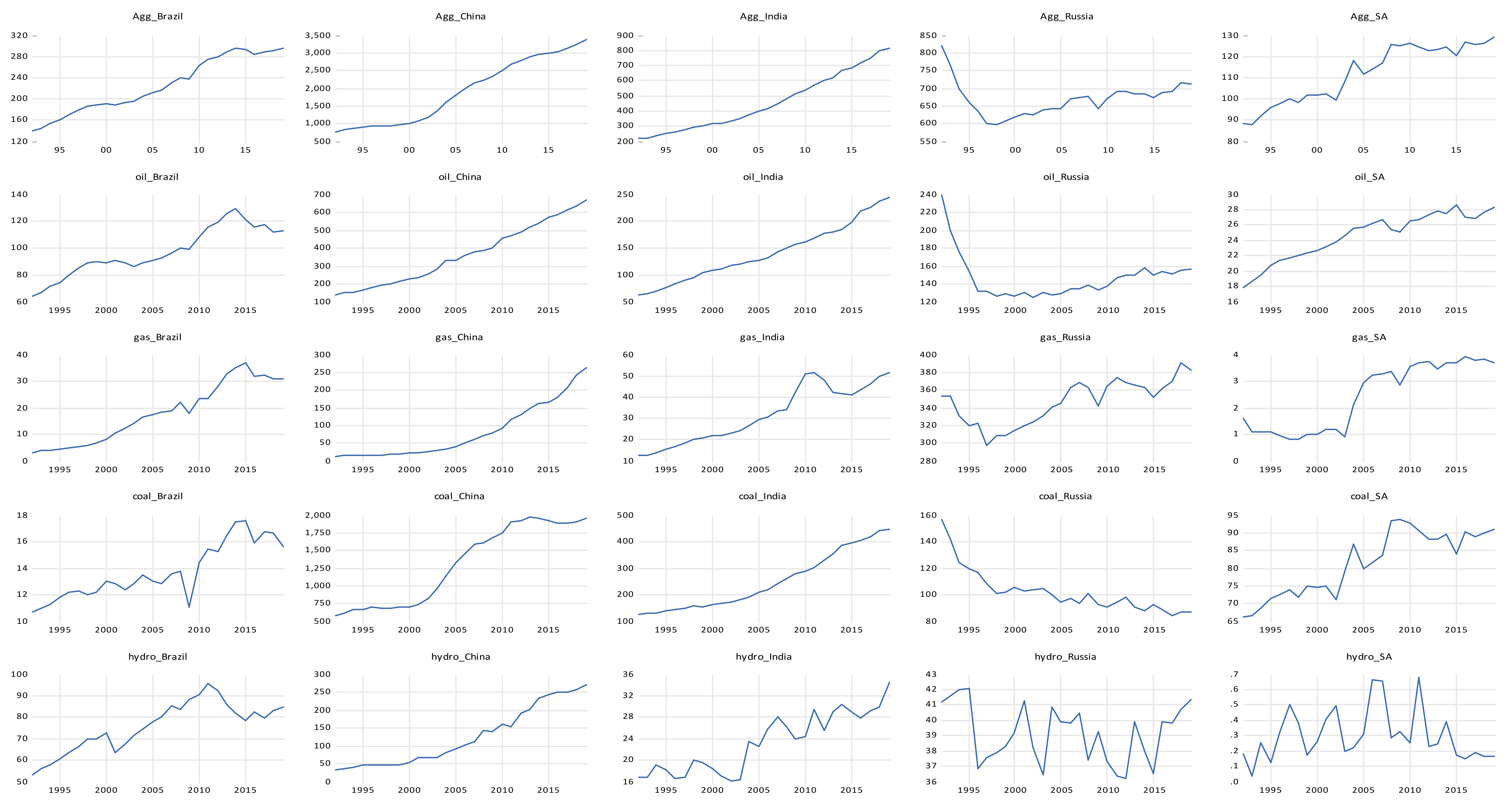
To begin the analysis, the time series are presented in Figure A1 in the Appendix. One can notice that in most cases, energy consumption was growing over time. Only in Russia, a decreasing trend is observed in coal energy consumption. Total (aggregate) energy consumption was decreasing in 1992–1998. Oil and gas consumption decreased in 1992–1996; since that time, a growing tendency has been observed.
The descriptive statistics of the selected aggregate and disaggregate energy consumption series of BRICS are provided in Table A1 in the Appendix. The mean value of “agg” ranges from 111.4 (mtoe) in South Africa to 1909.42 (mtoe) in China, in BRICS countries. However, the mean value of “coal” ranges from 13.71 in Brazil to 1298.20 in China. Similarly, the average “gas” is lowest in South Africa with 2.42, while it is highest in Russia with 346.38. On the other hand, average “hydro” is lowest in South Africa with 0.30 and highest in China with 123.78. Finally, average “oil” is lowest in South Africa with 24.55, while it is highest in China with 360.67 mtoe.
As far as variability, measured by the standard deviation, is concerned, the BRICS countries are pretty diversified, according to different energy sources. South Africa has the smallest value (13.51 mtoe), while China has the highest value (919.14 mtoe) for aggregate energy consumption. China exhibits maximum variability for aggregate and disaggregates time series (coal, gas, oil, and hydro). The variability coefficients expressed as standard deviation/mean ratio, amounted from 42.9% for “coal” to 94.7% for “gas”. It is related to the highest energetic expansion of the Chinese economy over the last four decades. India shows the second-highest variability coefficients. The amount from 23.8% for oil to 42.4% for gas. Russia exhibits the most negligible variability (from 4.8% for hydro to 16.9% for oil).
The study testing for normality using Jarque and Bera test [88] indicates that most of the time series satisfied the normal distribution. Only aggregate energy consumption and coal energy consumption in Russia do not fulfill this condition. The departures from normality do not deteriorate the results. In the case of , a normal distribution is not assumed. It is necessary for estimating the parameters. However, when the number of observations is relatively tiny (T = 28), such deviations are admissible.
The unit root characteristics of the time series are presented in Table A2. Most cases confirmed the unit root hypothesis apart from four series, i.e., Russia’s “agg”, “coal” and “hydro” energy, and South Africa’s “hydro” energy, which were stationary. In the case of China’s “gas” and “oil” the order of integration was bigger than one. In these cases, was not applicable.
2.2. Methodology
The current study is based on grey model. The model was introduced to the literature in 2019. Its application to energy consumption forecasting is still not recognized by the authors of the paper [1] based on simulation results. In the current study, the model is compared to a standard model, as well as the widely recognized in the forecasting literature. We focus on model comparison in terms of forecasting ability.
2.2.1. Unit Root Testing and ARIMA (p,d,q) Model
The most recognized representation for nonstationary time series is the model that can be written in the form:
where , and are polynomials in the lag operator, , defined such that , , is the unconditional mean, is the order of integer differencing, and is a white noise process (i.i.d. normally distributed) (for further details, see [3,89]). This model is termed an to indicate lags in the and lags in the terms, and is an integer differencing. To estimate the parameters of the model, the maximum likelihood method is recommended. The model selection procedure, related to lag parameters and , is based on the Akaike information criterion (AIC) and Bayesian information criterion (BIC) [90]. model refers to integrated time series, which become stationary after d-th times differencing. To determine whether a time series is stationary or not, the Augmented Dickey and Fuller test is typically used [91].
2.2.2. Fractional-Order GM (1, 1) Model
The construction of the fractional-order grey model methodology is explained by [1]. As it is quite a new approach, it is presented in this Section.
Definition 1.
The sequence of raw data series iswhere, which is known as,,,……,is the r th-order accumulating sequence of,,……, [55] where is denoting the gamma function,
Definition 2.
Assume thatis the sequence of raw data, where, which is known as,, ……,is the rth order reducing generation sequence of [55]. where,
Definition 3.
Assume that,,…,is defined as Definition 1, and,,………, is followed the Definition 2.
Thus, ,,………,, where
The model formula
is representing the . The FGM(1,1) introduced a fractional-order r, which can take non-integer values. The following conditions are distinguished: if r = 1, Equation is representing the
Which is called as standard grey model described in [2] if r = 0, Equation is representing the direct modeling.
It is expected that the development coefficient to be negative and the intension parameter to be positive (See, [92] chapter 7, p. 149).
2.2.3. Forecasting Accuracy Measures
The most popular measures of forecast accuracy concentrate on computing forecast errors. There are plenty of such measures, such as MSE and MAPE (See, [93] (p. 309). Their usefulness consists of showing the differences in accuracy of computed forecasts but say nothing about the method of forecasting.
In 1995, ref. [4] derived a testing procedure of equal predictive accuracy. The hypothesis to be tested says that the alternative methods are equally accurate on average. The general idea of Diebold-Mariano’s test relies on two-time series, including actual values and forecasts of a predicted variable, say and , as well as on the loss function depending on the forecast and actual values only through the forecast error, defined as: . The loss function may take many different forms, which is discussed further in this part. What we compare is a loss differential between the two forecasts, coming from two competing models of the form: . The forecasting methods are equally accurate if , which is assumed under the null hypothesis.
This paper applied the Diebold-Mariano test to compare a standard model, , and model estimated for different values. The loss function based on the mean square error was selected for comparison because the differences between forecast errors were relatively low. It is worth emphasizing that such a comparison is possible only if a sufficient number of observations are necessary to estimate the model.
3. Results
The results of forecasting energy consumption using the model are presented in Table 1 for aggregate energy consumption and in Table A3, Table A4, Table A5 and Table A6 for disaggregates energy consumption. All results of aggregate and disaggregate energy consumption is reported with the following values: MAPE, MSE, development coefficient (), and grey input ( In the different () values are applied. In the study, r = {− 1.5; − 0.9; − 0.5; − 0.1; − 0.05; − 0.01; 0; 0.01; 0.05; 0.1; 0.5; 0.9; 1; 1.5}.
In Table 1, the results of aggregate energy consumption are reported. The minimum MAPE values were taken as the main criterion of model selection. Additionally, the assumptions for a < 0 and b > 0 were to be fulfilled. For Brazil, the order () is = 0.9 with the minimum MAPE= 3.43; for China, the order () is = 0.5 with the minimum MAPE= 10.030; for India, the order () is =1 with the minimum MAPE = 2.163, and for Russia, the order () is = 1 with the minimum MAPE = 3.632. Finally, South Africa has the least MAPE = 21.565 with the parameters , and where the value of = 0.
In Table A4, the results of gas consumption are reported. For Brazil, the order () is = 0.1 with the minimum MAPE = 22.262 with the appropriate sign of grey parameters. For China, the order () is = 1 with the minimum MAPE = 18.884; for India, the order () is = 0.1 with the minimum MAPE =7.842, and for Russia, the order () is = 1 with the minimum MAPE = 3.408. For South Africa, the best model is for the value of = 0.9. It has the least MAPE = 30.042.
In Table A5, the results of coal consumption are reported. For Brazil, the order () is = 1 with the minimum MAPE = 8.040, for China, the order () is = 0.5 with the minimum MAPE = 13.971, for India, the order () is = 1 with the minimum MAPE = 4.489, and for Russia, the order () is = 1.5 with the minimum MAPE = 12.986. South Africa has the least MAPE = 3.335, where the value of = 0.9.
Finally, in Table A6, the results of hydro energy consumption are reported. For Brazil, the order () is = 0.9 with the minimum MAPE = 5.552. For China, the order () is = 1 with the minimum MAPE = 11.418, for India, the order () is = 1 with the minimum MAPE = 8.642, for Russia, the order () is = 1.5 with the minimum MAPE = 14.648, and for South Africa, the order () is = 1.5 with the least MAPE = 122.067.
Summing up, the most frequently model with r = 0.9 and r = 1 were supported by the data. Quite often, the following values: r = 1.5 and r = 0.1 were indicated. Moreover, r = 0.5 was shown twice and r = 0 once. It means that the model outperformed the in terms of energy consumption prediction since it allows more flexible fitting to the time series’ actual values. As r = 1 corresponds to the , one can notice that this model is quite valuable for energy consumption prediction.
As mentioned in Section 2.2.3, the results of forecasting can be compared, and the models’ effectiveness in prediction can be evaluated using the Diebold-Mariano test. The results of the model comparison are presented in Table 2.
The conclusion of model comparison using the Diebold-Mariano test is that the for many values of r, , and possess an equal predictive ability for energy consumption forecasting in BRICS countries. This is a universal conclusion, since if the observation number is large, one can rely on both the stochastic time series model like ARIMA and grey type models. As concerns , for small negative r values like −1.5, the results are much worse. This conclusion is useful because one can limit the range of possible values between (− 1.00; + 1.00). The two results (China, hydro = 0.00 and India coal, = − 0.05), when the null hypothesis of equal predictive ability was rejected, can be considered random.
4. Discussion
BRICS countries belong to the developing economies group, although China has become a global competitor in some areas [94]. Developing countries desire precise forecasts of both scales of growth and energy consumption. They also need to optimize energy exploitation from different sources and adopt new technologies for renewable energy sources. As the economy grows, energy consumption increases as well. It is a danger in increasing energy consumption over a very long time. According to the law of entropy, the resources are limited, and too much recycling will result in energy waste [95]. Proponents of ecological economics consider the problem of sustainability to be that of sustainable macroeconomic scale, acknowledging the possibility that the economy may become or may already be so large that it places demands on the environment exceeding its carrying capacity [96].
However, there are strict limitations to energy consumption. They divide into global and country-specific limitations. Global recommendations origin is in the United Nations’ 2030 Agenda for the Sustainable Development Goals (SDGs), which all 193 UN member states accepted. Among 17 SDGs, goal 7 assumes access to affordable, reliable, sustainable, and modern energy for all, and goal 13 covers urgent action to combat climate change and its impacts. Country-specific limitations consist of natural resource exploitation, technology for energy production, and transformation and consciousness of the necessity of rationalization. Considering the above, the energy policy of BRICS countries needs continuous monitoring for forecasting accuracy and its structure according to the SDGs requirements. The most important policy recommendation is to shift energy consumption from fossil fuels (oil, gas, coal, oil shales, etc.) to renewable energy consumption. The less usage of fossil fuel will be more beneficial for the environment by providing environmental awareness.
The results of the grey and models’ comparison presented in the current paper revealed as follows:
- Fractional Grey Model allows a broad spectrum of parameters that adjust to the empirical data. An FGM-based approach is more comprehensive than the standard model, which is “a special case” of for = 1.
- According to the Diebold-Mariano test results, the estimated models taking parameters’ range (−1; 1) confirmed equal predictive ability with model as well as model.
- Although grey-type models are mostly recommended for short time series, their predictive ability is equal to models designed for long time series. However, taking values of MSE and MAPE in empirical study, model highly outperformed in 19 cases on 25. In six cases, were not applicable. For Chinese oil and gas consumption, the time series was integrated of higher order than one. The remaining four series were stationary.
- For some parameter “” values, empirical models do not satisfy the grey model assumption, i.e., and . In such circumstances, it is recommended to estimate the model for another “” parameter value.
- Grey-type models are helpful for forecasting in the case when only a few observations are available. Still, for long and nonstationary time series, standard time series models perform better.
In the paper [97], the authors provided a methodological comparison of probability models, fuzzy math, grey systems, and rough sets. It appears that grey models are evidently preferred in the case of small samples and incomplete information sets. They concentrate on the law of reality. On the other hand, stochastic models, such as are designed for large samples and follow historical law. The general conclusion that both types of models possess equal predictive ability indicated by the Diebold-Mariano test allows selecting the proper procedure for a given data set and forecasting perspective. The exact values of MAPE and MSE are less informative because they are valid only for a given sample. Therefore, the presented results are in line with both theory and expectations.
5. Conclusions
The BRICS are emerging economies concerning the production and management of resources and require a consistent supply of having energy resources. The BRICS countries should monitor energy consumption, focusing on the supply-demand gap of energy and its components and facilities provided to local and foreign investors. Therefore, forecasting is quite significant for energetic policy projection. Accurate forecasts of energy consumption are vital when demand grows faster. On the other hand, BRICS’s energy consumption values can be offered as fluctuating and increasing.
This study aimed to predict energy consumption in BRICS. Firstly, this paper focused on forecasting the annual energy consumption for BRICS using two types of models. It compared , and models by estimating the errors (MAPE) and (MSE) in the years 1992–2019. Secondly, the results have revealed that outperformed when in-sample estimating errors are compared. Thirdly, model comparison using the Diebold-Mariano test confirmed the equal predictive ability of and unless the FGM parameter ranges (− 1, 1). The results allow concluding that if the number of observations is large enough, stochastic models such as and grey models such as FGM are helpful for energy consumption forecasting. The procedure enabled narrowing the range of possible parameter values for r in the Fractional .
Moreover, the empirical findings allow formulating some recommendations. BRICS countries need to follow SDGs concerning energetic policy keeping their economic growth level increasing. It implies a gradual structural change from traditional towards renewable energy sources. A structural change always means a significant limitation of the number of observations; therefore, the model is recommended for predicting energy consumption in aggregate and disaggregate levels.
Author Contributions
Conceptualization, A.M.K., and M.O.; methodology, A.M.K. and M.O.; software, A.M.K. and M.O.; validation, M.O.; formal analysis, A.M.K.; investigation, A.M.K.; resources, A.M.K.; data curation, A.M.K.; writing—original draft preparation, A.M.K., and M.O.; writing—review and editing, A.M.K., and M.O.; visualization, A.M.K., and M.O. All authors have read and agreed to the published version of the manuscript.
Funding
Not applicable.
Acknowledgments
We would like to thank Wei Meng for providing the code for Fractional-order GM (1, 1) method and for valuable guidance.
Conflicts of Interest
The authors declare no conflict of interest.
Appendix A

Table A1.
Summary statistics of energy consumption for BRICS in 1992–2019.
| Brazil | Russia | India | China | South Africa | |||||||||||||||||||||
|---|---|---|---|---|---|---|---|---|---|---|---|---|---|---|---|---|---|---|---|---|---|---|---|---|---|
| Variable | Agg | Oil | Gas | Coal | Hydro | Agg | Oil | Gas | Coal | Hydro | Agg | Oil | Gas | Coal | Hydro | Agg | Oil | Gas | Coal | Hydro | Agg | Oil | Gas | Coal | Hydro |
| Mean | 224.48 | 97.12 | 17.87 | 13.72 | 75.63 | 668.91 | 146.39 | 346.38 | 102.32 | 39.16 | 456.45 | 140.38 | 31.60 | 249.51 | 23.24 | 1909.42 | 360.69 | 81.16 | 1298.20 | 123.78 | 111.94 | 24.55 | 2.42 | 81.39 | 0.30 |
| Med | 214.21 | 91.52 | 17.54 | 13.00 | 78.15 | 670.93 | 137.99 | 352.03 | 99.16 | 39.55 | 405.72 | 129.09 | 30.18 | 215.24 | 23.71 | 1892.64 | 346.59 | 45.04 | 1389.66 | 95.99 | 115.44 | 25.47 | 2.91 | 82.57 | 0.26 |
| Max | 296.25 | 129.59 | 36.92 | 17.62 | 95.44 | 819.31 | 238.82 | 390.80 | 156.98 | 42.10 | 813.50 | 244.53 | 51.84 | 444.73 | 34.46 | 3384.43 | 666.52 | 264.26 | 1969.07 | 270.33 | 129.00 | 28.62 | 3.91 | 93.82 | 0.68 |
| Min | 139.15 | 64.37 | 3.19 | 10.68 | 53.34 | 598.74 | 125.21 | 297.00 | 83.93 | 36.20 | 218.18 | 63.79 | 12.41 | 123.67 | 16.16 | 758.40 | 134.64 | 13.68 | 578.80 | 31.21 | 88.12 | 17.92 | 0.80 | 66.35 | 0.03 |
| S. D. | 52.31 | 18.04 | 11.20 | 2.09 | 11.44 | 48.43 | 24.75 | 24.91 | 16.69 | 1.89 | 188.65 | 53.38 | 13.40 | 108.11 | 5.53 | 919.14 | 167.76 | 76.87 | 557.56 | 81.93 | 13.51 | 3.05 | 1.25 | 8.99 | 0.17 |
| Ske | 0.04 | 0.05 | 0.19 | 0.46 | -0.27 | 1.05 | 2.24 | −0.26 | 1.75 | −0.08 | 0.47 | 0.39 | 0.12 | 0.53 | 0.16 | 0.16 | 0.30 | 0.98 | −0.05 | 0.54 | −0.33 | −0.65 | −0.14 | −0.19 | 0.98 |
| Kurt | 1.61 | 2.07 | 1.66 | 1.98 | 2.09 | 4.77 | 8.47 | 2.01 | 5.97 | 1.71 | 1.90 | 2.15 | 1.57 | 1.83 | 1.72 | 1.44 | 1.77 | 2.73 | 1.24 | 1.78 | 1.63 | 2.31 | 1.20 | 1.59 | 3.19 |
| J-B | 2.25 | 1.03 | 2.28 | 2.19 | 1.29 | 8.78 | 58.27 | 1.45 | 24.65 | 1.98 | 2.44 | 1.53 | 2.45 | 2.91 | 2.03 | 2.96 | 2.16 | 4.59 | 3.62 | 3.09 | 2.72 | 2.50 | 3.86 | 2.50 | 4.53 |
| Prob | 0.32 | 0.60 | 0.32 | 0.33 | 0.52 | 0.01 | 0.00 | 0.48 | 0.00 | 0.37 | 0.29 | 0.46 | 0.29 | 0.23 | 0.36 | 0.23 | 0.34 | 0.10 | 0.16 | 0.21 | 0.26 | 0.29 | 0.15 | 0.29 | 0.10 |
| Obs. | 28 | 28 | 28 | 28 | 28 | 28 | 28 | 28 | 28 | 28 | 28 | 28 | 28 | 28 | 28 | 28 | 28 | 28 | 28 | 28 | 28 | 28 | 28 | 28 | 28 |
Note: Med: Median; Max = Maximum; Min=Minimum; S.D. = Standard deviation; Ske = Skewness; Kurt = Kurtosis; J-B = Jarque-Berra; Prob = Probability; Ob s = Observations.
Table A2.
Unit Root (ADF) Testing for BRICS in 1992–2019.
| Brazil | Russia | India | China | South Africa | ||||||||||||||||||||||
|---|---|---|---|---|---|---|---|---|---|---|---|---|---|---|---|---|---|---|---|---|---|---|---|---|---|---|
| Variable | Agg | Oil | Gas | Coal | Hydro | Agg | Oil | Gas | Coal | Hydro | Agg | Oil | Gas | Coal | Hydro | Agg | Oil | Gas | Coal | Hydro | Agg | Oil | Gas | Coal | Hydro | |
| Level | Statistic | −0.992 | 0.101 | −0.718 | −1.575 | −1.882 | −3.761 | −2.499 | −0.859 | −3.421 | −3.403 | −0.822 | 2.436 | −0.801 | 2.449 | −0.598 | 0.227 | 2.157 | 3.298 | −0.801 | 1.651 | −1.282 | −2.214 | −0.539 | −1.513 | −3.760 |
| Prob. | 0.741 | 0.958 | 0.826 | 0.481 | 0.335 | 0.009 * | 0.127 | 0.785 | 0.020 * | 0.020 * | 0.950 | 1.000 | 0.802 | 1.000 | 0.855 | 0.969 | 1.000 | 1.000 | 0.801 | 0.999 | 0.623 | 0.206 | 0.868 | 0.512 | 0.009 * | |
| First difference | Statistic | −4.052 | −4.186 | −3.516 | −5.597 | −4.586 | −3.286 | −4.259 | −4.843 | −3.707 | −5.383 | −6.050 | −3.713 | −3.653 | −3.373 | −5.749 | −2.202 | −4.722 | 0.605 | −2.556 | −6.243 | −5.892 | −5.038 | −4.671 | −5.908 | −4.463 |
| Prob. | 0.005 * | 0.004 * | 0.018 * | 0.000 * | 0.001 * | 0.026 * | 0.003 * | 0.001 * | 0.011 * | 0.000 * | 0.000 * | 0.010 * | 0.012 * | 0.022 * | 0.000 * | 0.210 * | 0.001 * | 0.986 | 0.116 | 0.000 * | 0.000 * | 0.000 * | 0.001 * | 0.000 * | 0.002 * | |
Note: * indicate the rejection of the null hypothesis of a unit root at the 1% significant levels, respectively; agg = aggregate. ADF test with intercept.
Figure A1.
Graphical trends of energy consumption for BRICS in 1992–2019.

Table A3.
Mean absolute percentage error (MAPE) and mean square error (MSE) for oil consumption of BRICS in 1992–2019.
Table A3.
Mean absolute percentage error (MAPE) and mean square error (MSE) for oil consumption of BRICS in 1992–2019.
| FGM (1, 1) for Brazil | ARIMA(1, 1, 1) | ||||||||||||||
| r = 0 | r = 0.01 | r = 0.05 | r = 0.1 | r = 0.5 | r = 0.9 | r = 1 | r = 1.5 | r = −0.01 | r = −0.05 | r = −0.1 | r = − 0.5 | r = − 0.9 | r = −1.5 | ||
| MSE | 49.603 | 49.386 | 115.761 | 52.035 | 61.483 | 42.264 | 47.209 | 554.869 | 50.008 | 54.215 | 66.398 | 55.720 | 57.320 | 13,798.910 | 12.622 |
| MAPE | 5.180 | 5.229 | 3.437 | 5.828 | 6.954 | 5.030 | 5.632 | 17.095 | 5.128 | 5.157 | 5.645 | 5.899 | 6.013 | 115.989 | 2.552 |
| a | 0.053 | 0.055 | 0.060 | 0.062 | 0.024 | −0.013 | −0.020 | − 0.050 | 0.051 | 0.038 | 0.014 | 0.525 | 1.234 | 2.701 | — |
| b | 6.992 | 7.501 | 9.428 | 11.640 | 29.519 | 60.981 | 73.023 | 181.164 | 6.471 | 4.276 | 1.513 | 9.415 | 3.614 | − 4.374 | — |
| FGM (1, 1) for China | |||||||||||||||
| r = 0 | r = 0.01 | r = 0.05 | r = 0.1 | r = 0.5 | r = 0.9 | r = 1 | r = 1.5 | r = −0.01 | r = −0.05 | r = -0.1 | r = −0.5 | r = −0.9 | r = −1.5 | ||
| MSE | 173.090 | 163.078 | 135.180 | 118.389 | 145.729 | 231.141 | 346.868 | 4,832.628 | 184.703 | 137.248 | 433.358 | 83,239.662 | 4709.281 | 93,920.959 | NA |
| MAPE | 3.866 | 3.716 | 3.198 | 2.795 | 3.745 | 4.356 | 5.595 | 14.754 | 4.025 | 3.894 | 6.633 | 80.335 | 23.117 | 90.676 | NA |
| a | −0.032 | −0.032 | −0.030 | −0.029 | −0.036 | −0.052 | −0.056 | −0.076 | − 0.033 | 0.004 | −0.039 | −0.028 | 1.073 | 1.877 | — |
| b | 8.143 | 8.747 | 11.243 | 14.555 | 51.763 | 124.539 | 152.515 | 403.135 | 7.548 | 4.943 | 2.562 | −2.197 | 28.462 | 0.568 | — |
| FGM (1, 1) for India | |||||||||||||||
| r = 0 | r = 0.01 | r = 0.05 | r = 0.1 | r = 0.5 | r = 0.9 | r = 1 | r = 1.5 | r = −0.01 | r = −0.05 | r = −0.1 | r = −0.5 | r = −0.9 | r = −1.5 | ||
| MSE | 24.484 | 26.001 | 32.126 | 39.551 | 53.420 | 17.790 | 21.358 | 653.221 | 22.992 | 18.043 | 26.741 | 1694.731 | 445.230 | 19,010.504 | 14.203 |
| MAPE | 3.248 | 3.343 | 3.651 | 4.148 | 5.602 | 2.457 | 3.206 | 15.675 | 3.140 | 2.741 | 3.453 | 33.074 | 15.496 | 96.138 | 2.112 |
| a | −0.038 | −0.037 | −0.032 | −0.028 | −0.027 | −0.042 | −0.046 | −0.067 | −0.039 | −0.045 | −0.054 | 0.147 | 1.464 | 2.613 | — |
| b | 1.392 | 1.704 | 2.987 | 4.670 | 22.514 | 56.272 | 69.239 | 185.918 | 1.084 | −0.109 | −1.493 | 4.815 | 13.837 | −0.474 | — |
| FGM (1, 1) for Russia | |||||||||||||||
| r = 0 | r = 0.01 | r = 0.05 | r = 0.1 | r = 0.5 | r = 0.9 | r = 1 | r = 1.5 | r = −0.01 | r = −0.05 | r = −0.1 | r = −0.5 | r = −0.9 | r = −1.5 | ||
| MSE | 188.868 | 212.817 | 371.977 | 751.580 | 235.376 | 339.298 | 282.710 | 189.970 | 168.724 | 112.864 | 73.178 | 53.418 | 3378.958 | 389,209.753 | 58.974 |
| MAPE | 8.593 | 9.093 | 11.887 | 17.409 | 8.047 | 9.725 | 8.781 | 5.566 | 8.143 | 6.758 | 5.526 | 4.440 | 39.446 | 436.351 | 4.332 |
| a | 0.389 | 0.364 | 0.236 | 0.047 | 0.030 | 0.006 | −0.001 | −0.034 | 0.412 | 0.484 | 0.549 | 1.111 | 2.091 | 2.527 | — |
| b | 53.226 | 51.381 | 37.649 | 8.659 | 41.620 | 115.046 | 140.362 | 361.965 | 54.558 | 56.147 | 53.643 | 22.856 | −0.617 | −18.040 | — |
| FGM (1, 1) for South Africa | |||||||||||||||
| r = 0 | r = 0.01 | r = 0.05 | r = 0.1 | r = 0.5 | r = 0.9 | r = 1 | r = 1.5 | r = −0.01 | r = −0.05 | r = −0.1 | r = −0.5 | r = −0.9 | r = −1.5 | ||
| MSE | 0.322 | 0.322 | 0.352 | 0.439 | 0.999 | 0.419 | 1.011 | 38.694 | 0.326 | 0.389 | 0.687 | 2.363 | 1.411 | 1311.244 | 0.223 |
| MAPE | 1.799 | 1.787 | 1.957 | 2.217 | 3.480 | 2.151 | 3.291 | 17.950 | 1.811 | 1.988 | 3.091 | 5.561 | 3.791 | 138.693 | 1.894 |
| a | 0.072 | 0.075 | 0.082 | 0.084 | 0.035 | −0.005 | −0.013 | −0.045 | 0.068 | 0.040 | −0.024 | 0.641 | 1.467 | 2.966 | — |
| b | 2.149 | 2.323 | 2.927 | 3.561 | 8.411 | 17.103 | 20.436 | 50.270 | 1.964 | 1.058 | −0.383 | 2.878 | 1.055 | −1.208 | — |
Note: MSE = Mean Standard Error; MAPE = Mean Absolute Percentage Error. The shaded area indicates the best model for a given country.
Table A4.
Mean absolute percentage error (MAPE) and mean square error (MSE) for gas consumption of BRICS in 1992–2019.
Table A4.
Mean absolute percentage error (MAPE) and mean square error (MSE) for gas consumption of BRICS in 1992–2019.
| FGM (1, 1) for Brazil | ARIMA(1, 1, 1) | ||||||||||||||
| r = 0 | r = 0.01 | r = 0.05 | r = 0.1 | r = 0.5 | r = 0.9 | r = 1 | r = 1.5 | r = −0.01 | r = −0.05 | r = −0.1 | r = −0.5 | r = −0.9 | r = −1.5 | ||
| MSE | 13.971 | 13.862 | 13.461 | 13.031 | 11.422 | 15.033 | 17.749 | 60.883 | 14.085 | 14.589 | 15.360 | 42.822 | 58.652 | 2234.459 | 4.822 |
| MAPE | 22.107 | 22.113 | 22.170 | 22.262 | 24.350 | 29.581 | 31.343 | 43.135 | 22.101 | 22.173 | 22.340 | 31.303 | 66.971 | 278.951 | 9.528 |
| a | 0.008 | 0.007 | 0.004 | −0.001 | −0.035 | −0.062 | −0.068 | −0.092 | 0.009 | 0.012 | 0.016 | 0.007 | 0.006 | 0.108 | — |
| b | 1.166 | 1.192 | 1.300 | 1.441 | 2.972 | 5.820 | 6.883 | 16.021 | 1.140 | 1.038 | 0.915 | 0.072 | −0.104 | −0.090 | — |
| FGM (1, 1) for China | |||||||||||||||
| r = 0 | r = 0.01 | r = 0.05 | r = 0.1 | r = 0.5 | r = 0.9 | r = 1 | r = 1.5 | r = −0.01 | r = −0.05 | r = −0.1 | r = −0.5 | r = −0.9 | r = −1.5 | — | |
| MSE | 2386.569 | 2286.868 | 1933.065 | 1576.655 | 422.742 | 236.068 | 233.796 | 455.330 | 2491.238 | 2964.885 | 3703.170 | 22,144.389 | 49,126.530 | 63,696.575 | NA |
| MAPE | 60.179 | 58.943 | 54.298 | 49.114 | 26.881 | 19.728 | 18.884 | 19.937 | 61.446 | 66.841 | 74.376 | 175.801 | 310.118 | 473.308 | NA |
| a | −0.108 | −0.108 | −0.108 | −0.109 | −0.115 | −0.122 | −0.124 | −0.133 | −0.108 | −0.107 | −0.107 | −0.098 | −0.054 | 0.067 | — |
| b | 0.756 | 0.787 | 0.920 | 1.101 | 3.377 | 8.018 | 9.794 | 25.724 | 0.725 | 0.608 | 0.477 | -0.092 | −0.046 | −0.445 | — |
| FGM (1, 1) for India | |||||||||||||||
| r = 0 | r = 0.01 | r = 0.05 | r = 0.1 | r = 0.5 | r = 0.9 | r = 1 | r = 1.5 | r = −0.01 | r = −0.05 | r = −0.1 | r = −0.5 | r = −0.9 | r = −1.5 | — | |
| MSE | 18.215 | 18.125 | 17.824 | 17.565 | 18.099 | 22.225 | 24.800 | 82.087 | 18.312 | 18.766 | 19.530 | 158.415 | 176.382 | 2806.706 | 4.925 |
| MAPE | 8.607 | 8.498 | 8.143 | 7.842 | 8.005 | 10.882 | 12.105 | 22.167 | 8.727 | 9.325 | 10.433 | 45.288 | 49.903 | 178.481 | 4.435 |
| a | −0.002 | −0.002 | −0.001 | −0.001 | −0.018 | −0.040 | −0.046 | −0.070 | −0.003 | −0.005 | −0.008 | 0.028 | 0.282 | 0.551 | — |
| b | 1.364 | 1.432 | 1.709 | 2.072 | 5.985 | 13.333 | 16.108 | 40.412 | 1.298 | 1.040 | 0.738 | 0.142 | 0.278 | −0.408 | — |
| FGM (1, 1) for Russia | |||||||||||||||
| r = 0 | r = 0.01 | r = 0.05 | r = 0.1 | r = 0.5 | r = 0.9 | r = 1 | r = 1.5 | r = −0.01 | r = −0.05 | r = −0.1 | r = −0.5 | r = −0.9 | r = −1.5 | — | |
| MSE | 1597.445 | 1070.673 | 199.004 | 149.132 | 594.394 | 338.965 | 211.700 | 4671.837 | 1708.874 | 804.480 | 274.693 | 262.158 | 1829.579 | 668,162.502 | 133.125 |
| MAPE | 11.005 | 8.753 | 3.498 | 2.980 | 5.601 | 4.213 | 3.408 | 13.490 | 11.384 | 7.178 | 4.153 | 4.028 | 11.768 | 229.299 | 2.555 |
| a | −0.042 | −0.046 | −0.019 | 0.021 | 0.039 | 0.001 | −0.008 | −0.041 | −0.028 | 0.152 | 0.402 | 0.793 | 1.639 | 2.507 | — |
| b | −13.414 | −14.730 | −3.854 | 16.874 | 120.034 | 257.855 | 309.562 | 770.353 | −8.978 | 43.940 | 99.941 | 45.230 | 9.518 | −25.102 | — |
| FGM (1, 1) for South Africa | |||||||||||||||
| r = 0 | r = 0.01 | r = 0.05 | r = 0.1 | r = 0.5 | r = 0.9 | r = 1 | r = 1.5 | r = −0.01 | r = −0.05 | r = −0.1 | r = −0.5 | r = −0.9 | r = −1.5 | — | |
| MSE | 0.551 | 0.539 | 0.496 | 0.454 | 0.315 | 0.330 | 0.350 | 0.687 | 0.563 | 0.622 | 0.718 | 1.937 | 2.245 | 36.106 | 0.057 |
| MAPE | 48.536 | 47.852 | 45.358 | 42.625 | 31.557 | 30.042 | 30.360 | 34.505 | 49.252 | 52.327 | 56.664 | 93.233 | 100.429 | 353.199 | 13.235 |
| a | −0.012 | −0.012 | −0.012 | −0.013 | −0.028 | −0.050 | −0.055 | −0.078 | −0.012 | −0.011 | −0.010 | 0.124 | 0.454 | 0.669 | — |
| b | 0.049 | 0.053 | 0.070 | 0.092 | 0.360 | 0.853 | 1.035 | 2.592 | 0.046 | 0.032 | 0.018 | 0.032 | 0.011 | −0.073 | — |
Note: MSE = Mean Standard Error; MAPE = Mean Absolute Percentage Error. The shaded area indicates the best model for a given country.
Table A5.
Mean absolute percentage error (MAPE) and mean square error (MSE) for coal consumption of BRICS in 1992-2019.
Table A5.
Mean absolute percentage error (MAPE) and mean square error (MSE) for coal consumption of BRICS in 1992-2019.
| FGM (1, 1) for Brazil | ARIMA(1, 1, 1) | ||||||||||||||
| r = 0 | r = 0.01 | r = 0.05 | r = 0.1 | r = 0.5 | r = 0.9 | r = 1 | r = 1.5 | r = −0.01 | r = −0.05 | r = −0.1 | r = −0.5 | r = −0.9 | r = −1.5 | ||
| MSE | 3.022 | 3.040 | 3.128 | 3.245 | 3.726 | 3.068 | 2.980 | 11.746 | 3.007 | 3.095 | 4.226 | 4.271 | 16.223 | 1863.829 | 0.763 |
| MAPE | 8.267 | 8.410 | 8.823 | 9.278 | 11.457 | 8.704 | 8.040 | 19.536 | 8.106 | 8.484 | 12.653 | 13.056 | 28.945 | 319.597 | 4.321 |
| a | 0.012 | 0.018 | 0.038 | 0.054 | 0.033 | −0.005 | −0.013 | −0.044 | 0.006 | −0.012 | −0.001 | 0.367 | 0.629 | 0.645 | — |
| b | 0.345 | 0.452 | 0.888 | 1.385 | 4.437 | 9.289 | 11.142 | 27.770 | 0.243 | −0.058 | −0.012 | 0.727 | −0.016 | −0.516 | — |
| FGM(1,1) for China | |||||||||||||||
| r = 0 | r = 0.01 | r = 0.05 | r = 0.1 | r = 0.5 | r = 0.9 | r = 1 | r = 1.5 | r = −0.01 | r = −0.05 | r = −0.1 | r = −0.5 | r = −0.9 | r = −1.5 | ||
| MSE | 40,148.271 | 39,558.183 | 37,475.784 | 35,439.618 | 31,570.931 | 37,702.083 | 41,820.481 | 133,382.202 | 40,767.469 | 43,544.982 | 47,717.402 | 17,5312.752 | 90,654.063 | 1,102,950.215 | 1980.428 |
| MAPE | 15.554 | 15.364 | 14.691 | 14.165 | 13.971 | 14.936 | 15.868 | 22.104 | 15.761 | 16.716 | 18.127 | 39.026 | 28.406 | 94.467 | 2.691 |
| a | 0.006 | 0.006 | 0.006 | 0.005 | −0.016 | -0.041 | −0.047 | −0.072 | 0.006 | 0.005 | 0.003 | 0.097 | 0.706 | 1.851 | --- |
| b | 58.656 | 61.412 | 72.762 | 87.674 | 246.587 | 538.901 | 648.459 | 1604.314 | 55.931 | 45.376 | 33.035 | 21.642 | 43.347 | −19.890 | --- |
| FGM(1,1) for India | |||||||||||||||
| r = 0 | r = 0.01 | r = 0.05 | r = 0.1 | r = 0.5 | r = 0.9 | r = 1 | r = 1.5 | r = −0.01 | r = −0.05 | r = −0.1 | r = −0.5 | r = −0.9 | r = −1.5 | ||
| MSE | 413.770 | 375.372 | 273.808 | 216.300 | 257.278 | 177.617 | 143.883 | 1153.488 | 459.400 | 746.177 | 1537.331 | 9666.674 | 3228.482 | 73,129.170 | 62.304 |
| MAPE | 8.160 | 7.632 | 6.039 | 5.535 | 7.020 | 5.436 | 4.489 | 8.385 | 8.732 | 11.729 | 17.242 | 45.917 | 25.595 | 115.115 | 2.511 |
| a | −0.040 | −0.040 | −0.038 | −0.036 | −0.037 | −0.050 | −0.054 | −0.072 | −0.041 | −0.043 | −0.047 | 0.126 | 1.237 | 2.362 | --- |
| b | 1.905 | 2.296 | 3.950 | 6.213 | 32.779 | 85.160 | 105.423 | 289.759 | 1.524 | 0.102 | −1.420 | 6.772 | 20.189 | −2.474 | --- |
| FGM(1,1) for Russia | |||||||||||||||
| r = 0 | r = 0.01 | r = 0.05 | r = 0.1 | r = 0.5 | r = 0.9 | r = 1 | r = 1.5 | r = −0.01 | r = −0.05 | r = −0.1 | r = −0.5 | r = −0.9 | r = −1.5 | ||
| MSE | 20.822 | 19.540 | 15.492 | 13.169 | 64.766 | 57.719 | 35.647 | 410.340 | 22.203 | 28.623 | 38.245 | 74.944 | 578.569 | 156,299.051 | NA |
| MAPE | 3.764 | 3.646 | 3.250 | 2.842 | 6.480 | 5.514 | 4.183 | 12.986 | 3.880 | 4.453 | 5.221 | 7.576 | 23.016 | 398.090 | NA |
| a | 0.253 | 0.245 | 0.210 | 0.141 | 0.095 | 0.026 | 0.015 | −0.027 | 0.261 | 0.293 | 0.334 | 0.866 | 1.898 | 2.453 | --- |
| b | 23.099 | 23.192 | 22.979 | 18.459 | 56.429 | 104.897 | 123.841 | 294.931 | 22.971 | 22.239 | 21.062 | 10.176 | −2.168 | −12.251 | --- |
| FGM(1,1) for South Africa | |||||||||||||||
| r = 0 | r = 0.01 | r = 0.05 | r = 0.1 | r = 0.5 | r = 0.9 | r = 1 | r = 1.5 | r = −0.01 | r = −0.05 | r = −0.1 | r = −0.5 | r = −0.9 | r = −1.5 | ||
| MSE | 14.173 | 13.693 | 12.783 | 13.175 | 23.058 | 14.400 | 17.494 | 392.652 | 14.761 | 17.875 | 36.789 | 31.934 | 27.484 | 19,716.100 | 11.116 |
| MAPE | 3.040 | 2.989 | 3.146 | 3.517 | 5.101 | 3.335 | 3.565 | 17.534 | 3.102 | 4.134 | 6.564 | 5.632 | 5.657 | 164.637 | 2.96 |
| a | 0.036 | 0.042 | 0.061 | 0.071 | 0.037 | −0.003 | −0.011 | −0.044 | 0.028 | −0.006 | 0.041 | 0.670 | 1.486 | 2.630 | --- |
| b | 3.818 | 4.591 | 7.336 | 10.128 | 28.091 | 57.857 | 69.193 | 170.402 | 3.015 | −0.081 | 2.354 | 9.554 | 2.946 | −4.523 | --- |
Note: MSE = Mean Standard Error; MAPE = Mean Absolute Percentage Error. The shaded area indicates the best model for a given country.
Table A6.
Mean absolute percentage error (MAPE) and mean square error (MSE) for hydroelectric consumption of BRICS in 1992–2019.
Table A6.
Mean absolute percentage error (MAPE) and mean square error (MSE) for hydroelectric consumption of BRICS in 1992–2019.
| FGM (1, 1) for Brazil | ARIMA(1, 1, 1) | ||||||||||||||
| r = 0 | r = 0.01 | r = 0.05 | r = 0.1 | r = 0.5 | r = 0.9 | r = 1 | r = 1.5 | r = −0.01 | r = −0.05 | r = −0.1 | r = −0.5 | r = −0.9 | r = −1.5 | ||
| MSE | 26.193 | 25.638 | 24.188 | 23.534 | 26.283 | 29.985 | 39.439 | 422.779 | 26.844 | 30.436 | 33.004 | 49.510 | 43.965 | 11,437.767 | 12.919 |
| MAPE | 4.903 | 4.871 | 4.786 | 4.766 | 5.250 | 5.552 | 6.888 | 20.785 | 4.951 | 5.228 | 5.451 | 7.822 | 7.371 | 134.446 | 3.7851 |
| a | 0.067 | 0.071 | 0.079 | 0.081 | 0.035 | −0.006 | −0.014 | −0.047 | 0.064 | 0.041 | 0.006 | 0.509 | 1.221 | 2.431 | — |
| b | 6.286 | 6.809 | 8.695 | 10.716 | 25.763 | 52.191 | 62.277 | 152.041 | 5.741 | 3.346 | 0.511 | 6.738 | 2.384 | −3.319 | — |
| FGM (1, 1) for China | |||||||||||||||
| r = 0 | r = 0.01 | r = 0.05 | r = 0.1 | r = 0.5 | r = 0.9 | r = 1 | r = 1.5 | r = −0.01 | r = −0.05 | r = −0.1 | r = −0.5 | r = −0.9 | r = −1.5 | ||
| MSE | 1,102,950.215 | 344.024 | 316.631 | 289.252 | 199.725 | 215.014 | 240.196 | 832.985 | 360.018 | 397.743 | 458.891 | 4067.114 | 10,319.203 | 36,363.546 | 97.298 |
| MAPE | 94.467 | 18.552 | 17.499 | 16.520 | 13.636 | 11.436 | 11.418 | 16.457 | 19.201 | 20.629 | 22.744 | 66.711 | 113.149 | 193.771 | 8.923 |
| a | 1.851 | −0.041 | −0.042 | −0.044 | −0.061 | −0.077 | −0.081 | −0.097 | −0.040 | −0.039 | −0.038 | −0.033 | 0.098 | 0.458 | — |
| b | −19.890 | 3.993 | 4.499 | 5.175 | 13.017 | 28.589 | 34.593 | 88.877 | 3.751 | 3.289 | 2.750 | −0.035 | 0.723 | −0.147 | — |
| FGM (1, 1) for India | |||||||||||||||
| r = 0 | r = 0.01 | r = 0.05 | r = 0.1 | r = 0.5 | r = 0.9 | r = 1 | r = 1.5 | r = −0.01 | r = −0.05 | r = −0.1 | r = −0.5 | r = −0.9 | r = −1.5 | ||
| MSE | 5.671 | 5.531 | 5.410 | 5.421 | 6.653 | 5.422 | 5.055 | 21.686 | 6.019 | 21.591 | 352.601 | 15.608 | 47.200 | 3145.920 | 4.534 |
| MAPE | 8.768 | 8.602 | 8.617 | 8.788 | 10.103 | 9.148 | 8.642 | 13.992 | 9.057 | 15.380 | 56.726 | 16.589 | 30.760 | 234.639 | 8.354 |
| a | −0.062 | −0.057 | −0.039 | −0.022 | 0.002 | −0.021 | −0.027 | -0.053 | −0.068 | −0.090 | −0.113 | 0.429 | 0.861 | 1.203 | — |
| b | −0.786 | −0.666 | −0.173 | 0.449 | 5.315 | 12.772 | 15.549 | 40.178 | −0.903 | −1.325 | −1.647 | 1.988 | 0.707 | −0.538 | — |
| FGM (1, 1) for Russia | |||||||||||||||
| r = 0 | r = 0.01 | r = 0.05 | r = 0.1 | r = 0.5 | r = 0.9 | r = 1 | r = 1.5 | r = −0.01 | r = −0.05 | r = −0.1 | r = −0.5 | r = −0.9 | r = −1.5 | ||
| MSE | 9.288 | 22.673 | 3.967 | 4.429 | 11.002 | 5.421 | 3.322 | 77.324 | 5.413 | 3.266 | 2.991 | 7.240 | 23.523 | 9454.585 | NA |
| MAPE | 6.744 | 10.793 | 4.074 | 4.359 | 7.240 | 5.056 | 4.248 | 14.648 | 4.782 | 4.036 | 3.762 | 5.829 | 11.862 | 242.602 | NA |
| a | −0.006 | −0.058 | −0.018 | 0.103 | 0.062 | 0.010 | 0.001 | −0.036 | 0.047 | 0.174 | 0.240 | 0.653 | 1.509 | 2.536 | — |
| b | −0.221 | −2.277 | −0.493 | 6.097 | 17.020 | 33.298 | 39.591 | 96.269 | 1.718 | 5.609 | 6.485 | 3.787 | 0.662 | −2.922 | — |
| FGM (1, 1) for South Africa | |||||||||||||||
| r = 0 | r = 0.01 | r = 0.05 | r = 0.1 | r = 0.5 | r = 0.9 | r = 1 | r = 1.5 | r = −0.01 | r = −0.05 | r = −0.1 | r = −0.5 | r = −0.9 | r = −1.5 | ||
| MSE | 0.049 | 0.047 | 0.041 | 0.036 | 0.024 | 0.026 | 0.028 | 0.049 | 0.050 | 0.054 | 0.054 | 0.026 | 0.454 | 28.255 | NA |
| MAPE | 54.051 | 51.839 | 50.271 | 51.327 | 58.643 | 67.637 | 72.447 | 122.067 | 56.466 | 63.976 | 67.613 | 78.740 | 293.018 | 1968.815 | NA |
| a | −0.005 | −0.002 | 0.011 | 0.030 | 0.067 | 0.014 | 0.003 | −0.040 | -0.008 | −0.016 | −0.022 | 0.013 | 0.040 | 0.035 | — |
| b | −0.002 | −0.001 | 0.005 | 0.016 | 0.136 | 0.269 | 0.317 | 0.729 | -0.003 | −0.007 | −0.009 | −0.007 | −0.007 | −0.006 | --- |
Note: MSE = Mean Standard Error; MAPE = Mean Absolute Percentage Error. The shaded area indicates the best model for a given country.
References
- Meng, W.; Zeng, B.; Li, S. A novel fractional-order grey prediction model and its modeling error analysis. Information 2019, 10, 167. [Google Scholar] [CrossRef] [Green Version]
- Deng, J.L. Basis on Grey System Theory; Huazhong University of Science and Technology Press: Wuhan, China, 2002. [Google Scholar]
- Box, G.E.; Jenkins, G.M.; Reinsel, G.C.; Ljung, G.M. Time Series Analysis: Forecasting and Control; John Wiley & Sons: Hoboken, NJ, USA, 2015. [Google Scholar]
- Diebold, F.X.; Mariano, R.S. Comparing predictive accuracy. J. Bus. Econ. Stat. 2002, 20, 134–144. [Google Scholar] [CrossRef]
- Oh, W.; Lee, K. Causal relationship between energy consumption and GDP revisited: The case of Korea 1970–1999. Energy Econ. 2004, 26, 51–59. [Google Scholar] [CrossRef]
- Altinay, G.; Karagol, E. Electricity consumption and economic growth: Evidence from Turkey. Energy Econ. 2005, 27, 849–856. [Google Scholar] [CrossRef]
- Lee, C.-C.; Chang, C.-P. Structural breaks, energy consumption, and economic growth revisited: Evidence from Taiwan. Energy Econ. 2005, 27, 857–872. [Google Scholar] [CrossRef]
- Soytas, U.; Sari, R. Energy consumption and GDP: Causality relationship in G-7 countries and emerging markets. Energy Econ. 2003, 25, 33–37. [Google Scholar] [CrossRef]
- Fatai, K.; Oxley, L.; Scrimgeour, F. Modelling the causal relationship between energy consumption and GDP in New Zealand, Australia, India, Indonesia, The Philippines and Thailand. Math. Comput. Simul. 2004, 64, 431–445. [Google Scholar] [CrossRef]
- Hatemi, A.; Irandoust, M. Energy consumption and economic growth in Sweden: A leveraged bootstrap approach, 1965–2000. Int. J. Appl. Econom. Quant. Stud. 2005, 2, 87–98. Available online: https://www.usc.gal/economet/Journals3/ijaeqs/ijaeqs246.pdf (accessed on 28 April 2021).
- Wolde-Rufael, Y. Electricity consumption and economic growth: A time series experience for 17 African countries. Energy Policy 2006, 34, 1106–1114. [Google Scholar] [CrossRef]
- Hor, C.-L.; Watson, S.J.; Majithia, S. Daily Load Forecasting and Maximum Demand Estimation using ARIMA and GARCH. In Proceedings of the 2006 International Conference on Probabilistic Methods Applied to Power Systems, Stockholm, Sweden, 11–15 June 2006; Volume 11, pp. 1–6. [Google Scholar]
- Miao, J. The Energy Consumption Forecasting in China Based on ARIMA Model. In Proceedings of the 2015 International Conference on Materials Engineering and Information Technology Applications, Guilin, China, 30–31 August 2015. [Google Scholar]
- Zhou, M.; Yan, Z.; Ni, Y.; Li, G.; Nie, Y. Electricity price forecasting with confidence-interval estimation through an extended ARIMA approach. IEE Proc. Gener. Transm. Distrib. 2006, 153, 187. [Google Scholar] [CrossRef]
- Wang, Q.; Li, S.; Li, R.; Ma, M. Forecasting U.S. shale gas monthly production using a hybrid ARIMA and metabolic nonlinear grey model. Energy 2018, 160, 378–387. [Google Scholar] [CrossRef]
- Wang, H.; Huang, J.; Zhou, H.; Zhao, L.; Yuan, Y. An Integrated Variational Mode Decomposition and ARIMA Model to Forecast Air Temperature. Sustainabilty 2019, 11, 4018. [Google Scholar] [CrossRef] [Green Version]
- Chai, J.; Lu, Q.-Y.; Wang, S.-Y.; Lai, K.K. Analysis of road transportation energy consumption demand in China. Transp. Res. Part D Transp. Environ. 2016, 48, 112–124. [Google Scholar] [CrossRef]
- Sen, P.; Roy, M.; Pal, P. Application of ARIMA for forecasting energy consumption and GHG emission: A case study of an Indian pig iron manufacturing organization. Energy 2016, 116, 1031–1038. [Google Scholar] [CrossRef]
- Yuan, C.; Liu, S.; Fang, Z. Comparison of China’s primary energy consumption forecasting by using ARIMA (the autoregressive integrated moving average) model and GM(1,1) model. Energy 2016, 100, 384–390. [Google Scholar] [CrossRef]
- De Assis Cabral, J.; Legey, L.F.L.; de Freitas Cabral, M.V. Electricity consumption forecasting in Brazil: A spatial econometrics approach. Energy 2017, 126, 124–131. [Google Scholar] [CrossRef]
- Ding, S.; Hipel, K.W.; Dang, Y.-G. Forecasting China’s electricity consumption using a new grey prediction model. Energy 2018, 149, 314–328. [Google Scholar] [CrossRef]
- Ma, M.; Wang, Z. Prediction of the Energy Consumption Variation Trend in South Africa based on ARIMA, NGM and NGM-ARIMA Models. Energies 2019, 13, 10. [Google Scholar] [CrossRef] [Green Version]
- Kumar, U.; Jain, V. Time series models (Grey-Markov, Grey Model with rolling mechanism and singular spectrum analysis) to forecast energy consumption in India. Energy 2010, 35, 1709–1716. [Google Scholar] [CrossRef]
- Julong, D. Introduction to grey system theory. J. Grey Syst. 1989, 1, 1–24. [Google Scholar]
- Xiao, X.; Yang, J.; Mao, S.; Wen, J. An improved seasonal rolling grey forecasting model using a cycle truncation accumulated generating operation for traffic flow. Appl. Math. Model. 2017, 51, 386–404. [Google Scholar] [CrossRef]
- Wu, X.; Mao, J.; Du, Z.; Chang, Y. Online training algorithms based single multiplicative neuron model for energy consumption forecasting. Energy 2013, 59, 126–132. [Google Scholar] [CrossRef]
- Ma, X.; Liu, Z. Application of a novel time-delayed polynomial grey model to predict the natural gas consumption in China. J. Comput. Appl. Math. 2017, 324, 17–24. [Google Scholar] [CrossRef]
- Lee, Y.-S.; Tong, L.-I. Forecasting energy consumption using a grey model improved by incorporating genetic programming. Energy Convers. Manag. 2011, 52, 147–152. [Google Scholar] [CrossRef]
- Yang, Y.; Xue, D. Continuous fractional-order grey model and electricity prediction research based on the observation error feedback. Energy 2016, 115, 722–733. [Google Scholar] [CrossRef]
- Yaoguo, D.; Sifeng, L.; Kejia, C. The GM models that x(n) be taken as initial value. Kybernetes 2004, 33, 247–254. [Google Scholar] [CrossRef]
- Li, M.; Wang, W.; De, G.; Ji, X.; Tan, Z. Forecasting carbon emissions related to energy consumption in beijing-tianjin-hebei region based on grey prediction theory and extreme learning machine optimized by support vector machine algorithm. Energies 2018, 11, 2475. [Google Scholar] [CrossRef] [Green Version]
- Pao, H.-T.; Fu, H.-C.; Tseng, C.-L. Forecasting of CO2 emissions, energy consumption and economic growth in China using an improved grey model. Energy 2012, 40, 400–409. [Google Scholar] [CrossRef]
- Feng, S.J.; Ma, Y.D.; Song, Z.L.; Ying, J. Forecasting the Energy Consumption of China by the Grey Prediction Model. Energy Sources Part B Econ. Plan. Policy 2012, 7, 376–389. [Google Scholar] [CrossRef]
- Li, W.; Xie, H. Geometrical Variable Weights Buffer GM(1,1) Model and Its Application in Forecasting of China’s Energy Consumption. J. Appl. Math. 2014, 2014, 1–6. [Google Scholar] [CrossRef]
- Fan, D.; Pang, C.; Kim, J.; Jon, S.; Gu, X. Forecasting the self-sufficiency rate of China’s energy by the hybrid gray models. Energy Sources, Part A: Recover. Util. Environ. Eff. 2019, 1–20. [Google Scholar] [CrossRef]
- Ju-Long, D. Control problems of grey systems. Syst. Control. Lett. 1982, 1, 288–294. [Google Scholar] [CrossRef]
- Wei, B.-L.; Xie, N.-M.; Yang, Y.-J. Data-based structure selection for unified discrete grey prediction model. Expert Syst. Appl. 2019, 136, 264–275. [Google Scholar] [CrossRef]
- Pi, D.; Liu, J.; Qin, X. A Grey prediction approach to forecasting energy demand in china. energy sources, Part A: Recover. Util. Environ. Eff. 2010, 32, 1517–1528. [Google Scholar] [CrossRef]
- Meng, X.Y.; Chen, R.H.; Bin Wang, S. The Metabolic GM (1, 1) prediction of the absolute gas emission quantity in a certain mine. Adv. Mater. Res. 2014, 989–994, 3480–3484. [Google Scholar] [CrossRef]
- Lu, H.Y. Application of GM (1, 1) prediction model in coal consumption market. Adv. Mater. Res. 2013, 869-870, 554–558. [Google Scholar] [CrossRef]
- Wang, Y.; Zheng, F.; He, K.; Li, C. Research of combination of electricity GM (1, 1) and seasonal time series forecasting model. In Proceedings of the Proceedings of the 4th International Conference on Information Technology and Management Innovation, Shenzhen, China, 12–13 September 2015. [Google Scholar]
- Xie, N.-M.; Yuan, C.-Q.; Yang, Y.-J. Forecasting China’s energy demand and self-sufficiency rate by grey forecasting model and Markov model. Int. J. Electr. Power Energy Syst. 2015, 66, 1–8. [Google Scholar] [CrossRef]
- Wang, Z.-X. A predictive analysis of clean energy consumption, economic growth and environmental regulation in china using an optimized grey dynamic model. Comput. Econ. 2015, 46, 437–453. [Google Scholar] [CrossRef]
- Liang, Y.; Niu, D.; Cao, Y.; Hong, W.-C. Analysis and modeling for china’s electricity demand forecasting using a hybrid method based on multiple regression and extreme learning machine: A view from carbon emission. Energies 2016, 9, 941. [Google Scholar] [CrossRef] [Green Version]
- Liang, J.; Liang, Y. Analysis and modeling for china’s electricity demand forecasting based on a new mathematical hybrid method. Information 2017, 8, 33. [Google Scholar] [CrossRef] [Green Version]
- Peng, G.; Wang, H.; Song, X.; Zhang, H. Intelligent management of coal stockpiles using improved grey spontaneous combustion forecasting models. Energy 2017, 132, 269–279. [Google Scholar] [CrossRef]
- Xu, N.; Dang, Y.; Gong, Y. Novel grey prediction model with nonlinear optimized time response method for forecasting of electricity consumption in China. Energy 2017, 118, 473–480. [Google Scholar] [CrossRef]
- Li, K.; Zhang, T. Forecasting electricity consumption using an improved grey prediction model. Information 2018, 9, 204. [Google Scholar] [CrossRef] [Green Version]
- Wei, B.; Xie, N.; Hu, A. Optimal solution for novel grey polynomial prediction model. Appl. Math. Model. 2018, 62, 717–727. [Google Scholar] [CrossRef]
- Pei, L.-L.; Li, Q. Forecasting Quarterly Sales Volume of the New Energy Vehicles Industry in China Using a Data Grouping Approach-Based Nonlinear Grey Bernoulli Model. Sustainability 2019, 11, 1247. [Google Scholar] [CrossRef] [Green Version]
- Meng, W.; Yang, D.; Huang, H. Prediction of China’s Sulfur Dioxide Emissions by Discrete Grey Model with Fractional Order Generation Operators. Complexity 2018, 2018, 1–13. [Google Scholar] [CrossRef] [Green Version]
- Shen, X.; Ou, L.; Chen, X.; Zhang, X.; Tan, X. The Application of the Grey Disaster Model to Forecast Epidemic Peaks of Typhoid and Paratyphoid Fever in China. PLoS ONE 2013, 8, e60601. [Google Scholar] [CrossRef] [Green Version]
- Wu, L.; Liu, S.; Yao, L.; Yan, S. The effect of sample size on the grey system model. Appl. Math. Model. 2013, 37, 6577–6583. [Google Scholar] [CrossRef]
- Xiong, P.-P.; Dang, Y.-G.; Yao, T.-X.; Wang, Z.-X. Optimal modeling and forecasting of the energy consumption and production in China. Energy 2014, 77, 623–634. [Google Scholar] [CrossRef]
- Liu, S.; Zeng, B.; Liu, J.-F.; Xie, N.; Yang, Y. Four basic models of GM(1, 1) and their suitable sequences. Grey Syst. Theory Appl. 2015, 5, 141–156. [Google Scholar] [CrossRef]
- Wu, L.; Liu, S.; Chen, H.; Zhang, N. Using a Novel Grey System Model to Forecast Natural Gas Consumption in China. Math. Probl. Eng. 2015, 2015, 1–7. [Google Scholar] [CrossRef]
- Zeng, B.; Meng, W.; Tong, M. A self-adaptive intelligence grey predictive model with alterable structure and its application. Eng. Appl. Artif. Intell. 2016, 50, 236–244. [Google Scholar] [CrossRef]
- Ma, X.; Hu, Y.-S.; Liu, Z.-B. A novel kernel regularized nonhomogeneous grey model and its applications. Commun. Nonlinear Sci. Numer. Simul. 2017, 48, 51–62. [Google Scholar] [CrossRef]
- Zeng, B.; Zhou, M.; Zhang, J. Forecasting the energy consumption of china’s manufacturing using a homologous grey prediction model. Sustainability 2017, 9, 1975. [Google Scholar] [CrossRef] [Green Version]
- Ma, X.; Liu, Z. The GMC (1, n) model with optimized parameters and its application. J. Grey Syst. 2017, 29, 122–138. [Google Scholar]
- Fan, G.-F.; Wang, A.; Hong, W.-C. Combining Grey Model and Self-Adapting Intelligent Grey Model with Genetic Algorithm and Annual Share Changes in Natural Gas Demand Forecasting. Energies 2018, 11, 1625. [Google Scholar] [CrossRef] [Green Version]
- Duan, H.; Lei, G.R.; Shao, K. Forecasting Crude Oil Consumption in China Using a Grey Prediction Model with an Optimal Fractional-Order Accumulating Operator. Complexity 2018, 2018, 1–12. [Google Scholar] [CrossRef]
- Wu, L.; Gao, X.; Xiao, Y.; Yang, Y.; Chen, X. Using a novel multi-variable grey model to forecast the electricity consumption of Shandong Province in China. Energy 2018, 157, 327–335. [Google Scholar] [CrossRef]
- Wu, W.; Ma, X.; Wang, Y.; Zhang, Y.; Zeng, B. Research on a novel fractional GM(α, n) model and its applications. Grey Syst. Theory Appl. 2019, 9, 356–373. [Google Scholar] [CrossRef]
- Wu, W.-Z.; Jiang, J.; Li, Q. A Novel Discrete Grey Model and Its Application. Math. Probl. Eng. 2019, 2019, 1–6. [Google Scholar] [CrossRef]
- Zhang, P.; Ma, X.; She, K. A novel power-driven fractional accumulated grey model and its application in forecasting wind energy consumption of China. PLoS ONE 2019, 14, e0225362. [Google Scholar] [CrossRef] [PubMed] [Green Version]
- Zeng, B.; Ma, X.; Zhou, M. A new-structure grey Verhulst model for China’s tight gas production forecasting. Appl. Soft Comput. 2020, 96, 106600. [Google Scholar] [CrossRef]
- Wang, H.; Yan, R.; Wang, Q.; Zhang, H. A Novel Approach to Forecast Electricity Consumption Based on Fractional Grey Model. In Proceedings of the 2020 39th Chinese Control Conference (CCC), Shenyang, China, 27–30 July 2020; pp. 2424–2428. [Google Scholar]
- Li, R.; Jiang, P.; Yang, H.; Li, C. A novel hybrid forecasting scheme for electricity demand time series. Sustain. Cities Soc. 2020, 55, 102036. [Google Scholar] [CrossRef]
- Luo, X.; Duan, H.; He, L. A Novel Riccati Equation Grey Model And Its Application In Forecasting Clean Energy. Energy 2020, 205, 118085. [Google Scholar] [CrossRef]
- Xiao, Q.; Gao, M.; Xiao, X.; Goh, M. A novel grey Riccati–Bernoulli model and its application for the clean energy consumption prediction. Eng. Appl. Artif. Intell. 2020, 95, 103863. [Google Scholar] [CrossRef]
- Xie, W.; Wu, W.-Z.; Liu, C.; Zhao, J. Forecasting annual electricity consumption in China by employing a conformable fractional grey model in opposite direction. Energy 2020, 202, 117682. [Google Scholar] [CrossRef]
- Cheng, M.; Li, J.; Liu, Y.; Liu, B. Forecasting Clean Energy Consumption in China by 2025: Using Improved Grey Model GM (1, N). Sustainability 2020, 12, 698. [Google Scholar] [CrossRef] [Green Version]
- Xie, W.; Wu, W.-Z.; Liu, C.; Zhang, T.; Dong, Z. Forecasting fuel combustion-related CO2 emissions by a novel continuous fractional nonlinear grey Bernoulli model with grey wolf optimizer. Environ. Sci. Pollut. Res. 2021, 1–17. [Google Scholar] [CrossRef]
- Hu, Y.; Ma, X.; Li, W.; Wu, W.; Tu, D. Forecasting manufacturing industrial natural gas consumption of China using a novel time-delayed fractional grey model with multiple fractional order. Comput. Appl. Math. 2020, 39, 1–30. [Google Scholar] [CrossRef]
- Zheng, C.; Wu, W.-Z.; Jiang, J.; Li, Q. Forecasting Natural Gas Consumption of China Using a Novel Grey Model. Complexity 2020, 2020, 1–9. [Google Scholar] [CrossRef]
- Wei, B.; Xie, N. On unified framework for discrete-time grey models: Extensions and applications. ISA Trans. 2020, 107, 1–11. [Google Scholar] [CrossRef]
- Wu, W.; Ma, X.; Wang, Y.; Cai, W.; Zeng, B. Predicting China’s energy consumption using a novel grey Riccati model. Appl. Soft Comput. 2020, 95, 106555. [Google Scholar] [CrossRef]
- Zheng, C.; Wu, W.-Z.; Xie, W.; Li, Q. A MFO-based conformable fractional nonhomogeneous grey Bernoulli model for natural gas production and consumption forecasting. Appl. Soft Comput. 2021, 99, 106891. [Google Scholar] [CrossRef]
- Es, H.A. Monthly natural gas demand forecasting by adjusted seasonal grey forecasting model. Energy Sources, Part A: Recover. Util. Environ. Eff. 2020, 43, 1–16. [Google Scholar] [CrossRef]
- Zheng, C.; Wu, W.-Z.; Xie, W.; Li, Q.; Zhang, T. Forecasting the hydroelectricity consumption of China by using a novel unbiased nonlinear grey Bernoulli model. J. Clean. Prod. 2021, 278, 123903. [Google Scholar] [CrossRef]
- Liu, C.; Wu, W.-Z.; Xie, W.; Zhang, J. Application of a novel fractional grey prediction model with time power term to predict the electricity consumption of India and China. Chaos, Solitons Fractals 2020, 141, 110429. [Google Scholar] [CrossRef]
- Wu, W.; Ma, X.; Zhang, Y.; Li, W.; Wang, Y. A novel conformable fractional non-homogeneous grey model for forecasting carbon dioxide emissions of BRICS countries. Sci. Total. Environ. 2020, 707, 135447. [Google Scholar] [CrossRef]
- Lee, Y.-S.; Tong, L.-I. Forecasting nonlinear time series of energy consumption using a hybrid dynamic model. Appl. Energy 2012, 94, 251–256. [Google Scholar] [CrossRef]
- Pao, H.-T.; Tsai, C.-M. Modeling and forecasting the CO2 emissions, energy consumption, and economic growth in Brazil. Energy 2011, 36, 2450–2458. [Google Scholar] [CrossRef]
- Trotter, I.M.; Bolkesjø, T.F.; Féres, J.G.; Hollanda, L. Climate change and electricity demand in Brazil: A stochastic approach. Energy 2016, 102, 596–604. [Google Scholar] [CrossRef]
- Li, D.-C.; Chang, C.-J.; Chen, C.-C.; Chen, W.-C. Forecasting short-term electricity consumption using the adaptive grey-based approach—An Asian case. Omega 2012, 40, 767–773. [Google Scholar] [CrossRef]
- Jarque, C.M.; Bera, A.K. Efficient tests for normality, homoscedasticity and serial independence of regression residuals. Econ. Lett. 1980, 6, 255–259. [Google Scholar] [CrossRef]
- Hamilton, J.D. Time Series Analysis; Princeton University Press: Princeton, NJ, USA, 1994. [Google Scholar]
- Wang, Y.; Liu, Q. Comparison of Akaike information criterion (AIC) and Bayesian information criterion (BIC) in selection of stock–recruitment relationships. Fish. Res. 2006, 77, 220–225. [Google Scholar] [CrossRef]
- Dickey, D.A.; Fuller, W.A. Distribution of the Estimators for Autoregressive Time Series with a Unit Root. J. Am. Stat. Assoc. 1979, 74, 427–431. [Google Scholar] [CrossRef]
- Liu, S.; Yang, Y.; Forrest, J. Grey Data Analysis: Methods, Models and Applications; Springer: Berlin/Heidelberg, Germany, 2016; Available online: https://0-link-springer-com.brum.beds.ac.uk/content/pdf/10.1007/978-981-10-1841-1.pdf (accessed on 28 April 2021).
- Rachev, S.T.; Mittnik, S.; Fabozzi, F.J.; Focardi, S.M. Financial Econometrics: From Basics to Advanced Modeling Techniques; John Wiley & Sons: Hoboken, NJ, USA, 2007. [Google Scholar]
- Tellis, A. The Return of U.S.-China Strategic Competition. In Strategic Asia 2020 U.S.-China Competition for Global Influence; Tellis, A., Szalwinski, A., Wills, M., Eds.; The National Bureau of Asian Research: Seattle, WA, USA; Washington, DC, USA. Available online: https://www.researchgate.net/publication/342014018_The_Return_of_US-China_Strategic_Competition (accessed on 31 March 2021).
- Schlegel, R.; Pfouts, R.W.; Hochwald, W.; Johnson, G.L. The Entropy Law and the Economic Process. J. Econ. Issues 1973, 7, 457–499. [Google Scholar] [CrossRef]
- McMahon, G.F.; Mrozek, J.R. Economics, entropy and sustainability. Hydrol. Sci. J. 1997, 42, 501–512. [Google Scholar] [CrossRef]
- Liu, S.; Forrest, J.; Yang, Y. A brief introduction to grey systems theory. Grey Syst. Theory Appl. 2012, 2, 89–104. [Google Scholar] [CrossRef]
Table 1.
Mean absolute percentage error (MAPE) and Mean Square Error (MSE) for Aggregate Energy Consumption of BRICS in 1992–2019.
Table 1.
Mean absolute percentage error (MAPE) and Mean Square Error (MSE) for Aggregate Energy Consumption of BRICS in 1992–2019.
| FGM (1, 1) for Brazil | ARIMA (1, 1, 1) | ||||||||||||||
| r = 0 | r = 0.01 | r = 0.05 | r=0.1 | r = 0.5 | r = 0.9 | r = 1 | r = 1.5 | r = −0.01 | r = −0.05 | r = −0.1 | r = −0.5 | r = −0.9 | r = −1.5 | ||
| MSE | 115.761 | 114.048 | 113.330 | 121.564 | 183.547 | 104.364 | 121.952 | 2365.346 | 118.233 | 137.248 | 194.597 | 120.572 | 153.293 | 71,846.171 | 34.952 |
| MAPE | 3.437 | 3.467 | 3.843 | 4.299 | 5.652 | 3.430 | 3.887 | 15.476 | 3.464 | 3.894 | 5.659 | 4.182 | 5.294 | 114.571 | 1.689 |
| a | 0.016 | 0.018 | 0.024 | 0.028 | 0.009 | −0.021 | 0.027 | −0.054 | 0.014 | 0.004 | −0.012 | 0.771 | 1.475 | 2.876 | — |
| b | 9.516 | 10.424 | 14.011 | 18.400 | 57.183 | 125.064 | 150.880 | 381.851 | 8.604 | 4.943 | 0.586 | 36.399 | 13.890 | −7.802 | — |
| FGM (1, 1) for China | |||||||||||||||
| r = 0 | r = 0.01 | r = 0.05 | r = 0.1 | r = 0.5 | r = 0.9 | r = 1 | r = 1.5 | r = −0.01 | r = −0.05 | r = −0.1 | r = −0.5 | r = −0.9 | r = −1.5 | ||
| MSE | 39,766.001 | 38,854.842 | 35,862.192 | 33,235.534 | 30,342.711 | 38,666.280 | 44,284.071 | 192,619.194 | 40,755.833 | 45,700.224 | 55,315.626 | 934,292.685 | 192,632.280 | 253,5304.295 | 1455.956 |
| MAPE | 11.649 | 11.426 | 10.681 | 10.145 | 10.030 | 10.567 | 11.432 | 17.974 | 11.882 | 12.919 | 14.596 | 62.912 | 29.165 | 96.097 | 1.889 |
| a | −0.021 | −0.021 | −0.020 | −0.020 | −0.033 | −0.052 | −0.056 | −0.077 | −0.021 | −0.022 | −0.025 | 0.019 | 0.842 | 2.014 | — |
| b | 57.208 | 60.395 | 73.612 | 91.213 | 288.417 | 665.437 | 808.421 | 2071.191 | 54.069 | 41.990 | 28.009 | 7.239 | 106.628 | −4.462 | — |
| FGM (1, 1) for India | |||||||||||||||
| r = 0 | r = 0.01 | r = 0.05 | r = 0.1 | r = 0.5 | r = 0.9 | r = 1 | r = 1.5 | r = −0.01 | r = −0.05 | r = −0.1 | r = −0.5 | r = −0.9 | r = −1.5 | ||
| MSE | 305.050 | 264.233 | 181.024 | 169.925 | 458.723 | 179.881 | 125.988 | 4767.086 | 358.196 | 775.327 | 2398.166 | 27,525.071 | 7235.069 | 231,705.058 | 75.811 |
| MAPE | 3.463 | 3.065 | 2.463 | 2.918 | 5.302 | 3.199 | 2.163 | 10.946 | 3.921 | 6.467 | 11.662 | 41.465 | 20.290 | 106.842 | 1.514 |
| a | −0.042 | −0.041 | −0.038 | −0.035 | −0.034 | −0.047 | −0.051 | −0.070 | −0.043 | −0.048 | −0.054 | 0.131 | 1.543 | 2.960 | — |
| b | 2.785 | 3.621 | 7.118 | 11.814 | 64.392 | 165.641 | 204.588 | 556.371 | 1.965 | −1.147 | −4.601 | 13.565 | 48.380 | −1.380 | — |
| FGM (1, 1) for Russia | |||||||||||||||
| r = 0 | r = 0.01 | r = 0.05 | r = 0.1 | r = 0.5 | r = 0.9 | r = 1 | r = 1.5 | r = −0.01 | r = −0.05 | r = −0.1 | r = −0.5 | r = −0.9 | r = −1.5 | ||
| MSE | 2557.965 | 3397.955 | 10,340.732 | 889.763 | 2634.297 | 2009.022 | 1210.561 | 13,152.140 | 1928.408 | 758.559 | 309.188 | 594.381 | 16,285.304 | NA | |
| MAPE | 6.689 | 7.659 | 15.072 | 3.786 | 5.938 | 4.659 | 3.632 | 11.189 | 5.825 | 3.619 | 2.245 | 3.203 | 18.722 | 293.588 | NA |
| a | 0.230 | 0.161 | −0.038 | −0.042 | 0.044 | 0.005 | −0.003 | −0.037 | 0.294 | 0.456 | 0.516 | 0.916 | 1.861 | 2.592 | — |
| b | 149.005 | 107.228 | −27.610 | −29.666 | 237.035 | 525.883 | 632.457 | 1,579.718 | 185.251 | 252.662 | 241.844 | 94.585 | 12.318 | −61.080 | — |
| FGM (1, 1) for South Africa | |||||||||||||||
| r = 0 | r = 0.01 | r = 0.05 | r = 0.1 | r = 0.5 | r = 0.9 | r = 1 | r = 1.5 | r = −0.01 | r = −0.05 | r = −0.1 | r = −0.5 | r = −0.9 | r = −1.5 | ||
| MSE | 314.658 | 313.896 | 314.996 | 321.056 | 365.344 | 322.015 | 312.152 | 809.537 | 316.329 | 347.810 | 469.286 | 497.888 | 1777.788 | 166,344.037 | 11.193 |
| MAPE | 21.565 | 21.750 | 22.218 | 22.419 | 23.788 | 22.161 | 21.932 | 31.946 | 21.368 | 22.720 | 28.334 | 29.611 | 52.934 | 444.068 | 2.294 |
| a | −0.001 | 0.003 | 0.018 | 0.033 | 0.027 | −0.008 | −0.015 | −0.046 | −0.005 | −0.013 | −0.002 | 0.336 | 0.587 | 0.604 | — |
| b | 1.376 | 1.962 | 4.654 | 8.259 | 33.693 | 72.221 | 86.774 | 216.973 | 0.845 | −0.527 | −0.133 | 5.297 | −0.143 | −3.801 | — |
Note: MSE = Mean Standard Error; MAPE = Mean Absolute Percentage Error. The shaded area indicates the best model for a given country. In Table A3, the results of oil consumption are reported. For Brazil, the order () is = 0.9 with the minimum MAPE = 5.030 with the appropriate sign of grey parameters. For China, the order () is = 0.1 with the minimum MAPE = 2.795. For India, the order () is = 0.9 with the minimum MAPE = 2.457. For Russia, the order () is = 1.5 with the minimum MAPE = 5.566. Finally, South Africa has the least MAPE = 2.151 where the value of = 0.9.
Table 2.
Diebold-Mariano test results (p-values) for comparison of GM (1, 1) and FGM (1, 1).
| GM(1,1) | Brazil | China | India | Russia | South Africa | ||||||||||||||||||||
|---|---|---|---|---|---|---|---|---|---|---|---|---|---|---|---|---|---|---|---|---|---|---|---|---|---|
| FGM(1,1) | Agg | Oil | Gas | Coal | Hydro | Agg | Oil | Gas | Coal | Hydro | Agg | Oil | Gas | Coal | Hydro | Agg | Oil | Gas | Coal | Hydro | Agg | Oil | Gas | Coal | Hydro |
| r = 0 | >0.1 | >0.1 | >0.1 | >0.1 | >0.1 | >0.1 | >0.1 | >0.1 | >0.1 | 0.044 | >0.1 | >0.1 | >0.1 | >0.1 | >0.1 | >0.1 | >0.1 | >0.1 | >0.1 | >0.1 | >0.1 | >0.1 | >0.1 | >0.1 | >0.1 |
| r = 0.01 | >0.1 | >0.1 | >0.1 | >0.1 | >0.1 | >0.1 | >0.1 | >0.1 | >0.1 | >0.1 | >0.1 | >0.1 | >0.1 | >0.1 | >0.1 | >0.1 | >0.1 | >0.1 | >0.1 | >0.1 | >0.1 | >0.1 | >0.1 | >0.1 | >0.1 |
| r = 0.05 | >0.1 | >0.1 | >0.1 | >0.1 | >0.1 | >0.1 | >0.1 | >0.1 | >0.1 | >0.1 | >0.1 | >0.1 | >0.1 | >0.1 | >0.1 | >0.1 | >0.1 | >0.1 | >0.1 | >0.1 | >0.1 | >0.1 | >0.1 | >0.1 | >0.1 |
| r = 0.1 | >0.1 | >0.1 | >0.1 | >0.1 | >0.1 | >0.1 | >0.1 | >0.1 | >0.1 | >0.1 | >0.1 | >0.1 | >0.1 | >0.1 | >0.1 | >0.1 | >0.1 | >0.1 | >0.1 | >0.1 | >0.1 | >0.1 | >0.1 | >0.1 | >0.1 |
| r = 0.5 | >0.1 | >0.1 | >0.1 | >0.1 | >0.1 | >0.1 | >0.1 | >0.1 | >0.1 | >0.1 | >0.1 | >0.1 | >0.1 | >0.1 | >0.1 | >0.1 | >0.1 | >0.1 | >0.1 | >0.1 | >0.1 | >0.1 | >0.1 | >0.1 | >0.1 |
| r = 0.9 | >0.1 | >0.1 | >0.1 | >0.1 | >0.1 | >0.1 | >0.1 | >0.1 | >0.1 | >0.1 | >0.1 | >0.1 | >0.1 | >0.1 | >0.1 | >0.1 | >0.1 | >0.1 | >0.1 | >0.1 | >0.1 | >0.1 | >0.1 | >0.1 | >0.1 |
| r = 1.5 | >0.1 | >0.1 | >0.1 | >0.1 | >0.1 | >0.1 | >0.1 | >0.1 | >0.1 | >0.1 | >0.1 | >0.1 | >0.1 | >0.1 | >0.1 | >0.1 | >0.1 | >0.1 | >0.1 | >0.1 | >0.1 | >0.1 | >0.1 | >0.1 | >0.1 |
| r= − 0.01 | >0.1 | >0.1 | >0.1 | >0.1 | >0.1 | >0.1 | >0.1 | >0.1 | >0.1 | >0.1 | >0.1 | >0.1 | >0.1 | >0.1 | >0.1 | >0.1 | >0.1 | >0.1 | >0.1 | >0.1 | >0.1 | >0.1 | >0.1 | >0.1 | >0.1 |
| r = − 0.05 | >0.1 | >0.1 | >0.1 | >0.1 | >0.1 | >0.1 | >0.1 | >0.1 | >0.1 | >0.1 | >0.1 | >0.1 | >0.1 | 0.040 | >0.1 | >0.1 | >0.1 | >0.1 | >0.1 | >0.1 | >0.1 | >0.1 | >0.1 | >0.1 | >0.1 |
| r = − 0.1 | >0.1 | >0.1 | >0.1 | >0.1 | >0.1 | >0.1 | >0.1 | >0.1 | >0.1 | >0.1 | >0.1 | >0.1 | >0.1 | >0.1 | >0.1 | >0.1 | >0.1 | >0.1 | >0.1 | >0.1 | >0.1 | >0.1 | >0.1 | >0.1 | >0.1 |
| r = − 0.5 | >0.1 | >0.1 | >0.1 | >0.1 | >0.1 | >0.1 | >0.1 | >0.1 | >0.1 | >0.1 | >0.1 | >0.1 | >0.1 | >0.1 | >0.1 | >0.1 | >0.1 | >0.1 | >0.1 | >0.1 | >0.1 | >0.1 | >0.1 | >0.1 | >0.1 |
| r = − 0.9 | >0.1 | >0.1 | >0.1 | >0.1 | >0.1 | >0.1 | >0.1 | >0.1 | >0.1 | >0.1 | >0.1 | >0.1 | >0.1 | >0.1 | >0.1 | >0.1 | >0.1 | >0.1 | >0.1 | >0.1 | >0.1 | >0.1 | >0.1 | >0.1 | >0.1 |
| r = − 1.5 | 0.020 | 0.022 | >0.1 | 0.024 | 0.021 | 0.016 | 0.019 | >0.1 | 0.048 | 0.040 | 0.027 | 0.038 | 0.024 | 0.024 | 0.026 | 0.015 | 0.012 | 0.015 | 0.015 | 0.024 | 0.023 | 0.029 | 0.039 | 0.020 | 0.000 |
| ARIMA (1, 1, 1) | >0.1 | >0.1 | >0.1 | >0.1 | >0.1 | >0.1 | NA | NA | >0.1 | >0.1 | >0.1 | >0.1 | >0.1 | >0.1 | >0.1 | NA | >0.1 | >0.1 | NA | NA | >0.1 | >0.1 | >0.1 | >0.1 | NA |
Note: Rejecting the null hypothesis is highlighted with the shaded area; agg = aggregate.
Publisher’s Note: MDPI stays neutral with regard to jurisdictional claims in published maps and institutional affiliations. |
© 2021 by the authors. Licensee MDPI, Basel, Switzerland. This article is an open access article distributed under the terms and conditions of the Creative Commons Attribution (CC BY) license (https://creativecommons.org/licenses/by/4.0/).
Share and Cite
MDPI and ACS Style
Khan, A.M.; Osińska, M. How to Predict Energy Consumption in BRICS Countries? Energies 2021, 14, 2749. https://0-doi-org.brum.beds.ac.uk/10.3390/en14102749
AMA Style
Khan AM, Osińska M. How to Predict Energy Consumption in BRICS Countries? Energies. 2021; 14(10):2749. https://0-doi-org.brum.beds.ac.uk/10.3390/en14102749
Chicago/Turabian StyleKhan, Atif Maqbool, and Magdalena Osińska. 2021. "How to Predict Energy Consumption in BRICS Countries?" Energies 14, no. 10: 2749. https://0-doi-org.brum.beds.ac.uk/10.3390/en14102749
Note that from the first issue of 2016, this journal uses article numbers instead of page numbers. See further details here.