
Transformer Fault Diagnosis Model Based on Improved Gray Wolf Optimizer and Probabilistic Neural Network


1
College of Qianhu, Nanchang University, Nanchang 330031, China
2
College of Information Engineering, Nanchang University, Nanchang 330031, China
*
Author to whom correspondence should be addressed.
Energies 2021, 14(11), 3029; https://0-doi-org.brum.beds.ac.uk/10.3390/en14113029
Submission received: 25 April 2021
/
Revised: 15 May 2021
/
Accepted: 19 May 2021
/
Published: 24 May 2021
/
Corrected: 4 April 2023
Abstract
:Dissolved gas analysis (DGA) based in insulating oil has become a more mature method in the field of transformer fault diagnosis. However, due to the complexity and diversity of fault types, the traditional modeling method based on oil sample analysis is struggling to meet the industrial demand for diagnostic accuracy. In order to solve this problem, this paper proposes a probabilistic neural network (PNN)-based fault diagnosis model for power transformers and optimizes the smoothing factor of the pattern layer of PNN by the improved gray wolf optimizer (IGWO) to improve the classification accuracy and robustness of PNN. The standard GWO easily falls into the local optimum because the update mechanism is too single. The update strategy proposed in this paper enhances the convergence ability and exploration ability of the algorithm, which greatly alleviates the dilemma that GWO is prone to fall into local optimum when dealing with complex data. In this paper, a reliability analysis of thirteen diagnostic methods is conducted using 555 transformer fault samples collected from Jiangxi Power Supply Company, China. The results show that the diagnostic accuracy of the IGWO-PNN model reaches 99.71%, which is much higher than that of the traditional IEC (International Electrotechnical Commission) three-ratio method. Compared with other neural network models, IGWO-PNN also has higher diagnostic accuracy and stability, and is more applicable to the field of transformer fault diagnosis.
1. Introduction
Power transformers are an important part of the power system [1,2]. Failure of power transformers may lead to interruption of power supply and loss of profit. Therefore, it is of great importance to detect early faults of power transformers accurately and in a timely manner so that they can be safely removed and the reliability of the power system can be improved [3,4].
At present, fault diagnosis techniques based on dissolved gas analysis are widely used in the field of oil-immersed power transformers [5], such as the IEC method [6], Rogers ratio method [7], Duval triangle method [8], and so on. Their applications in the field of oil-immersed power transformer fault diagnosis have been more mature. However, the classical fault diagnosis techniques often rely on the experienced judgment of professional technicians, and diagnosis accuracy is difficult to guarantee when the fault information is not comprehensive. Fault diagnosis algorithms based on data-driven technology have more numerous advantages over classical methods in terms of diagnostic accuracy and efficiency. Statistical-related methods, such as fuzzy theory [9], correlation analysis [10], hidden Markov model [11], support vector machine [12], and time series [13], have played an important role in transformer fault diagnosis models. With the development of machine learning techniques, artificial neural networks (ANN) [14], extreme learning machines (ELM) [15], back-propagation neural networks (BPNN) [16], and adaptive encoders [17], many other supervised and unsupervised neural network models are used in the field of fault diagnosis.
The above methods have achieved certain achievements compared with the traditional DGA fault diagnosis techniques. However, there are still many problems. For example, Li and Zhang et al. [12] use GA algorithm to modify the parameters in SVM, which significantly improves the classification accuracy of SVM. However, because SVM itself is a binary classification algorithm, there are some limitations in solving the multi classification problem. Compared with neural network algorithm, GA-SVM still has low diagnosis accuracy; the ANN-based fault diagnosis model [14] needs to set a large number of parameters, such as the topology of the network and the initial value of weights and thresholds. The process is cumbersome, and it is easy to fall into the local optimal situation in the face of complex centralized data, and the classification accuracy is not stable; the BP neural network has good generalization ability and fault tolerance, but the convergence speed of BP neural network algorithm is slow, and it is easy to fall into the problem of over fitting. In [16], a bat algorithm is used to optimize the parameters of BP neural network, which solves the problem of slow convergence of BPNN. However, the problem of low generalization ability of BPNN after training is not well solved in the established model. A probabilistic neural network (PNN) is a supervised neural network commonly used in pattern recognition, and its learning process mainly adopts probability density function estimation and Bayesian classification rules. The PNN model has parallel distributed processing, self-learning, and self-organization, as well as good potential for application in fault diagnosis. Compared with other neural network learning methods, it has faster convergence and better fault tolerance when the training samples are the same.
However, the network parameters of PNN (e.g., connection weights and pattern layer smoothing factors) largely determine the performance of the network, and selecting the most appropriate network parameters based on training data often optimizes the classification performance of PNN [18,19]. Manually adjusting the network parameters is not a good approach: the workload is tedious and it is also difficult to adjust the network parameters to the most suitable values. The addition of the optimization-seeking algorithm makes this task much easier and greatly improves the chances of finding the optimal parameters. Intelligent optimization algorithms such as particle swarm algorithm (PSO) [20], genetic algorithm (GA) [21], cuckoo search algorithm (CS) [22], and bat algorithm (BA) [23] have shown powerful capabilities in the optimization search of models, but also exposed the problem that the algorithms tend to fall into local optimum.
In this paper, a transformer fault diagnosis model based on Gray Wolf Optimizer (GWO) and Probabilistic Neural Network (PNN) is proposed. The GWO has the advantages of simple structure and high convergence compared with other intelligent algorithms. To avoid GWO from falling into the local optimum, this paper proposes a competitive update mechanism to improve the standard GWO. First, the standard update mechanism of GWO is modified to enhance the competitiveness of the standard update mechanism by modifying the convergence factor, and at the same time, a new search method is introduced for updating. The two update methods are compared based on the fitness values of the updated locations, and the location with better fitness performance is used as the final updated location. The improved Gray Wolf Optimizer (IGWO) is used to correct the smoothing factor of the PNN and optimize the classification performance of the PNN. Through experimental comparison with other neural network models, it is demonstrated that the proposed method can significantly improve the accuracy of fault diagnosis with high reliability and practicality.
This paper is divided into five sections: The first section summarizes the related work. The second section introduces the machine learning algorithm proposed in this paper. The third section describes the simulation model of transformer fault diagnosis that is established. In the fourth section, the experimental results are presented and discussed. Finally, the conclusion is drawn in the fifth section.
2. Method
2.1. IEC Three-Ratio Method
The IEC Three-Ratio Method is based on the dissolved gas analysis and the characteristic gas method. The five gases involved in this method are CH, CH, CH, H, and CH, which are characterized in the form of ratios (CH/CH, CH/H, and CH/CH) to identify faults [24]. The types of faults presented in this paper and the corresponding range of characteristic gas ratios can be represented by Table 1.
2.2. Improved Gray Wolf Optimizer
The Gray Wolf Optimizer (GWO) is a meta-heuristic algorithm proposed by Mirjalili et al. in 2014, academics from Griffith University, Australia. The algorithm was developed as an optimization search method inspired by the prey hunting activities of Gray wolves, and it has strong convergence performance, few parameters, and easy implementation [25].
The standard GWO optimization process is as follows: three wolves with the best fitness , , and lead -wolves to seek the best solution in the search space. This approach leads to slow convergence of GWO, premature loss of diversity in the population, and a tendency to fall into local optimal solutions. To overcome these problems, this section introduces an updating strategy called dimension learning-based hunting (DLH) [26] and modifies the convergence factor in the standard updating mechanism described above. After the standard update mechanism of GWO searches to get an update position, DLH searches again and gets another update position, and that with better fitness performance is selected as the final position. Such a strategy greatly improves the global search capability of GWO and reduces the possibility of the algorithm falling into a local optimum. The specific implementation steps of the improved Gray Wolf Optimizer are as follows.
Step 1: Initialization stage. N wolves in the population are randomly distributed in the search space within the given range of Equation (1):
where , denote the upper and lower bounds of the search space, respectively; rand [0,1] denotes a random number between 0 and 1. The matrix of N rows and d columns denoted by stores the positions of all gray wolf individuals in the population and defines this matrix as P. The fitness value of is calculated by the fitness function.
Step 2: The standard GWO location update mechanism. After initialization, the position update is first performed using the standard GWO update mechanism. The positions of all wolves in the population are updated based on the positions of , , and as a guide. First, as shown in Equation (2), the distances between the current -wolves and , , and are calculated separately.
where is the current position of wolf; , , represent the current distances between , , , and other individuals, respectively. , , and represent the current positions of , , and , respectively.
Second, the step lengths and directions of the wolves in the population advancing towards , , and are defined by Equation (3).
where , , and represent the updated positions of individuals under the guidance of , , and , respectively.
Finally, the final update position of individuals in the standard update mechanism, , is obtained by Equation (4).
Note that in Equations (2) and (3), , , and , , are coefficient vectors, which are calculated as follows:
where T is the maximum number of iterations set. a is a convergence factor that decreases linearly from 2 to 0 with the number of iterations. and are random numbers between [0, 1]. Considering that the convergence factor a decreases linearly in the iterative process of standard GWO, the linear decrement does not explain the algorithm’s optimization search process well. In this paper, we propose a new nonlinear convergence factor update method based on the change of exponential law. The exponential-based update method makes the convergence factor change more smoothly with iterations and enhances the ability of the algorithm to search globally. The update method is shown in Equation (8).
where and denote the upper and lower bounds of the convergence factor change, respectively, which are set by humans.
Step 3: DLH search mechanism. In hunting, the wolf pack will not only be updated by the guidance of the three wolves at the head to get a position , but also be influenced by the surrounding neighboring wolves to update the position, and we use to denote the updated gray wolf position through DLH. The Euclidean distance between and the original position of individual gray wolves is calculated first:
then a set of is constructed using Equation (10), which is denoted by .
where P is the gray wolf population position matrix mentioned earlier, i.e., the set composed of . denotes the Euclidean distance between and . In other words, we construct a circle domain with as the center and as the radius, and is the set consisting of gray wolf individuals in this circle domain except for and .
After constructing , the DLH search can be performed using Equation (11) to update the individual positions.
where m denotes the dimension in which the gray wolf location is located, and denote the randomly selected gray wolf locations from and P, respectively; and denotes the updated gray wolf location by DLH.
Step 4: Calculate the fitness values of and , respectively, and select the smaller fitness value as the final updated position. The mathematical expression is shown in Equation (12).
where and are the fitness values of and , respectively; denotes the final updated obtained position.
The whole process of IGWO can be represented by Algorithm 1.
| Algorithm 1 Pseudocode of the modified IGWO algorithm |
|
2.3. Brief Introduction of Probabilistic Neural Network
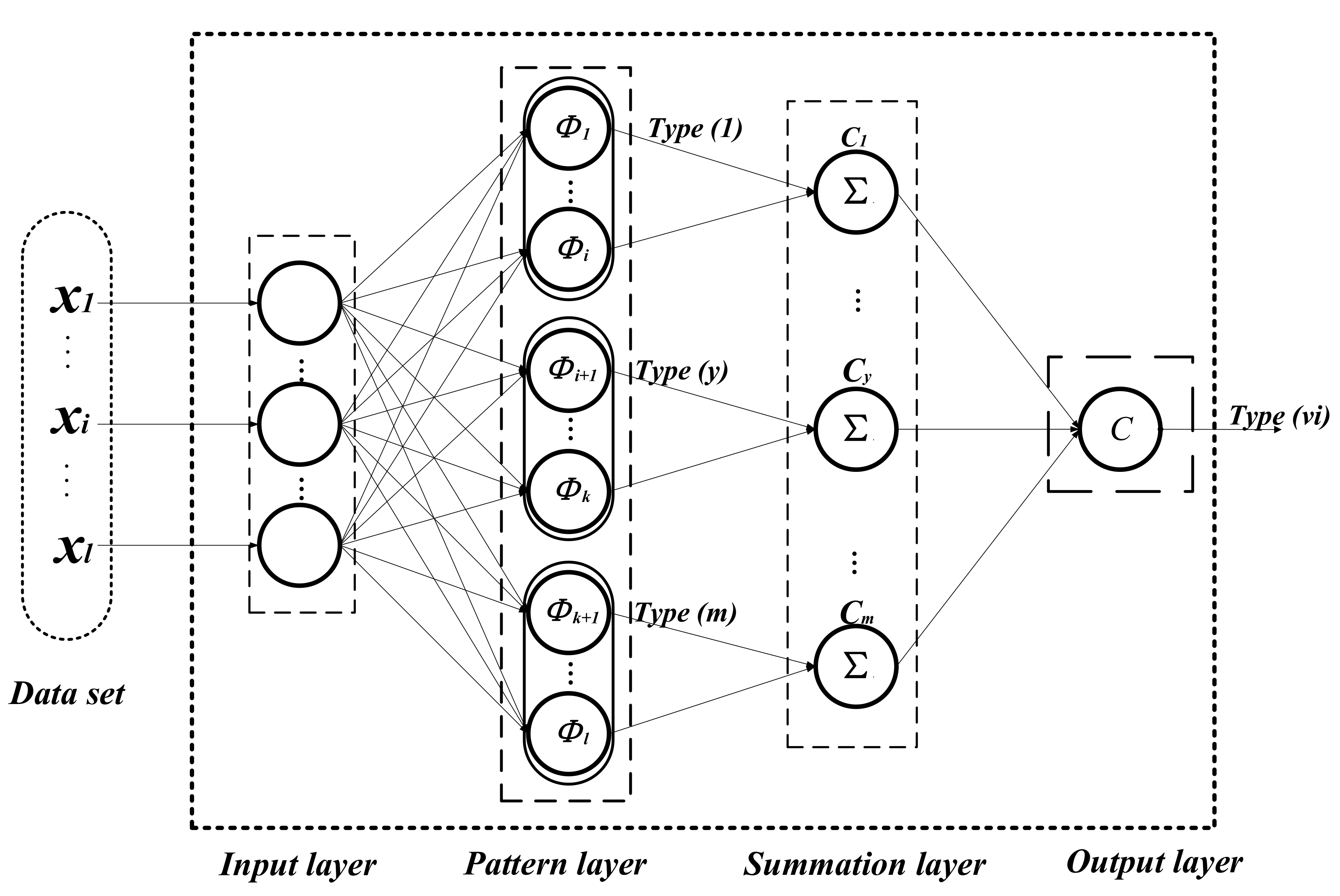
A probabilistic neural network (PNN) is a supervised learning model machine learning recognition algorithm. The principle of PNN algorithm is mainly based on Bayesian minimal risk decision theory and artificial neural network (ANN) model [27]. The PNN contains four layers of network structure, which are the input layer, implicit layer, summation layer, and output layer. Its structure diagram is shown in Figure 1.
The specific steps of PNN to achieve pattern classification are described as follows.
The original characteristic parameters of the data samples (denoted by x) are input by the input layer and multiplied with the weights to obtain the scalar . The mathematical model is expressed in Equation (13) as follows:
The number of neurons in the hidden layer is the number of input sample vectors, and each neuron node contains a center. Inputting into the pattern layer, the input–output relationship corresponding to the j-th neuron of the i-th sample in the hidden layer is
where denotes the smoothing factor, d denotes the dimension of the data sample, z is the input vector that needs to be identified, denotes the j-th center of the i-th sample, and denotes the output corresponding to the j-th neuron of the i-th sample in the pattern layer [28].
In the summation layer, the number of neurons is equal to the number of pattern categories. The summation layer obtains the probability density by taking a weighted average of the outputs of the implicit neurons of the same class in the pattern layer. The mathematical expression is as in Equation (15).
represents the output of type i and L represents the number of neurons of type i. Finally, according to the classification rules of Bayesian decision, each category corresponds to the evaluation of probabilities. The maximum posterior probability category is output by the output layer and the output is as follows:
2.4. Improved Gray Wolf Optimizer Based on Probabilistic Neural Network (IGWO-PNN)
The classification performance of PNN is easily affected by the smoothing factor () of the implied layer. Too large or too small a value of can significantly reduce the classification accuracy of PNN. In this paper, we build a PNN fault diagnosis model (IGWO-PNN) based on DGA data and use IGWO to optimize the smoothing factor of PNN to improve and stabilize the classification accuracy of PNN. The specific modeling process of IGWO-PNN is as follows.
Step 1: Input the training sample X from the input layer of PNN. The representation of X is shown in Equation (17):
where n and l are the dimensionality and the number of groups of the input samples, respectively.
Step 2: Initialize the IGWO parameters, population size N, dimensionality d, maximum number of iterations T, and set the fitness function fit(x) as required by the problem. In our model, the mean square error (MSE) is set as the fitness value and the corresponding fitness function can be expressed as
where is the actual output after training through the network and is the expected output.
Step 3: Initialize the probabilistic neural network parameters. A smoothing factor position matrix is randomly defined by Equation (9) in the search space, as shown in Equation (19):
where the matrix of smoothing factors represented by Equation (19) is equivalent to the matrix P stored in the gray wolf population.
Step 4: Calculate the fitness of each smoothing factor position in each of the N sets of smoothing factors by Equation (18) and record the three groups with the best current fitness, denoted as , , and , respectively.
Step 5: Calculate the convergence factor a by Equation (10);
Step 6: Iterate through the N sets of smoothing factors in Equation (19), calculate and for each set of smoothing factors, and select the one with the smaller fitness as the final updated position of this set of smoothing factors.
Step 7: After the traversal is completed, update the smoothing factor position matrix.
Step 8: If the maximum iteration condition (t <= T) is satisfied, continue to the next step; otherwise, return to Step 4.
Step 9: The optimized smoothing factor is fed into the PNN network for training to obtain the best PNN fault diagnosis model under the dataset.
Step 10: The test samples are fed into the network instead of the training samples to get the predicted fault type results.
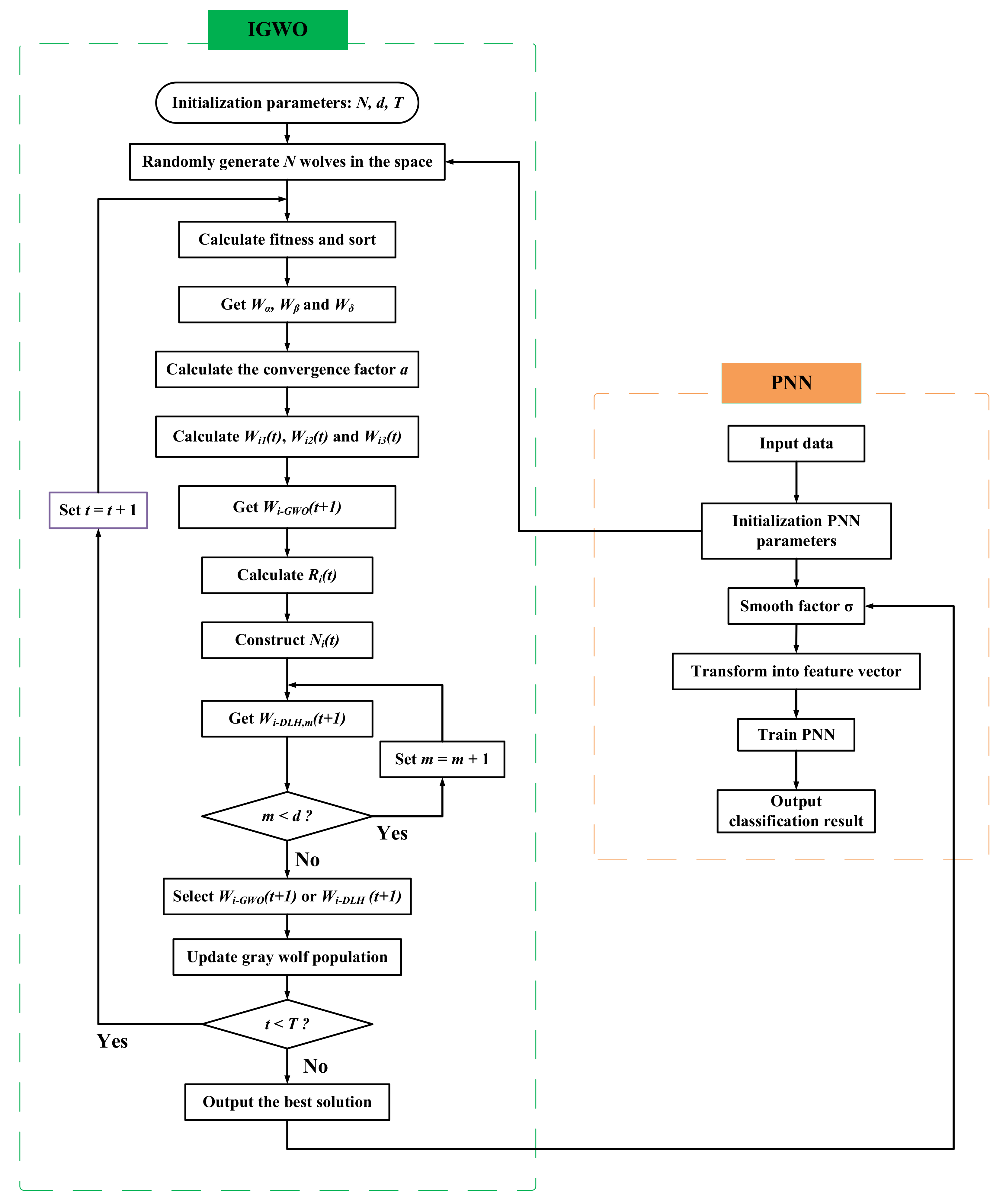
To facilitate readers’ understanding, we draw a flow chart as shown in Figure 2, which visually and clearly shows the whole process of IGWO-PNN.
3. Establishment of the Experiment
3.1. Model Implementation
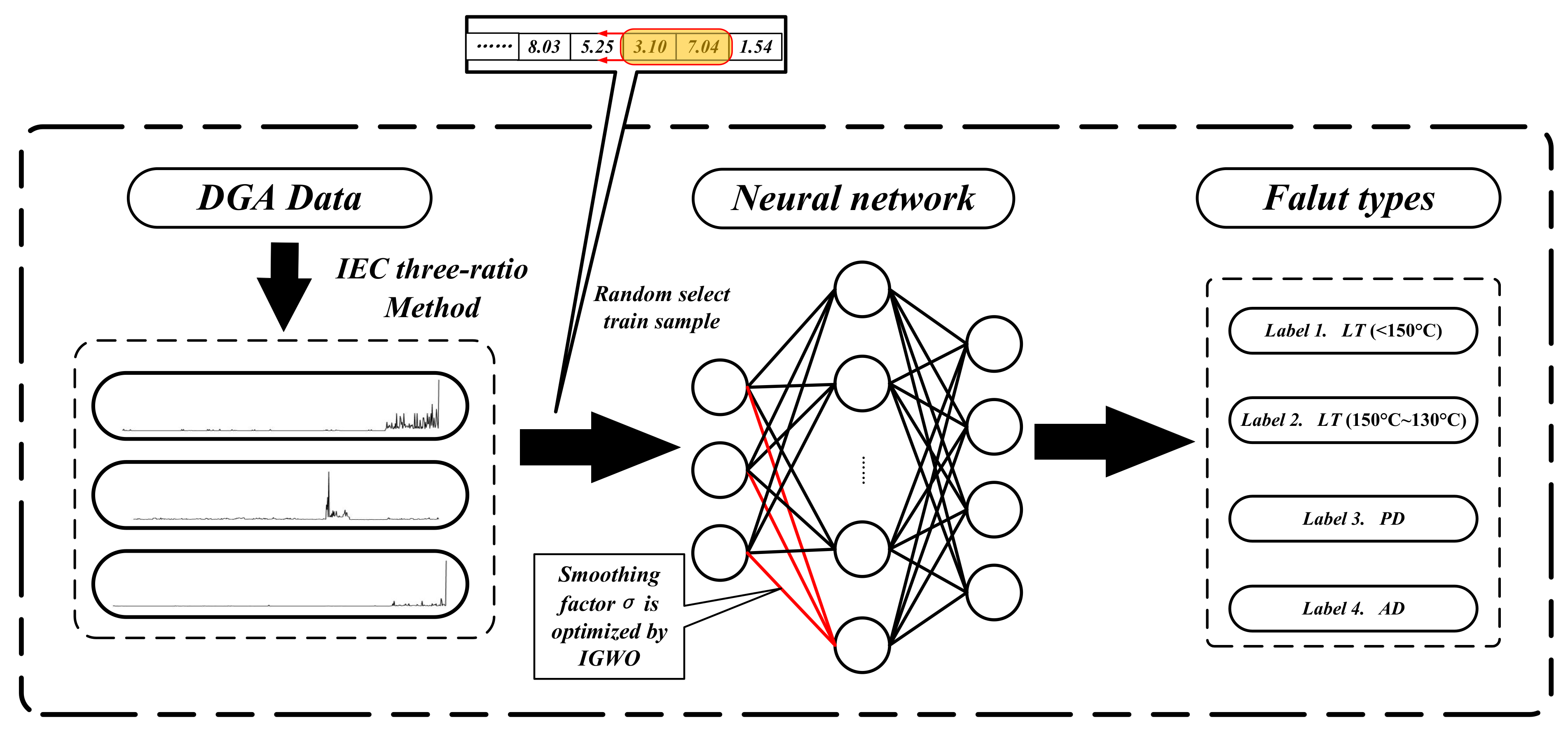
To verify the effectiveness of the proposed IGWO-PNN classification model in the field of transformer fault diagnosis, a specific power transformer fault diagnosis model was established based on the actual operating data of the transformer. First, the DGA data of the power transformer are acquired through smart sensors, and then the acquired sensor data are preprocessed by the three-ratio method. After that, the data are fed into the proposed classifier based on the machine learning method for training. Finally, the predicted classification results of the test set are obtained and the diagnostic accuracy is sought against the actual fault classes. The general flow is shown in Figure 3.
3.2. Data Acquisition and Preprocessing
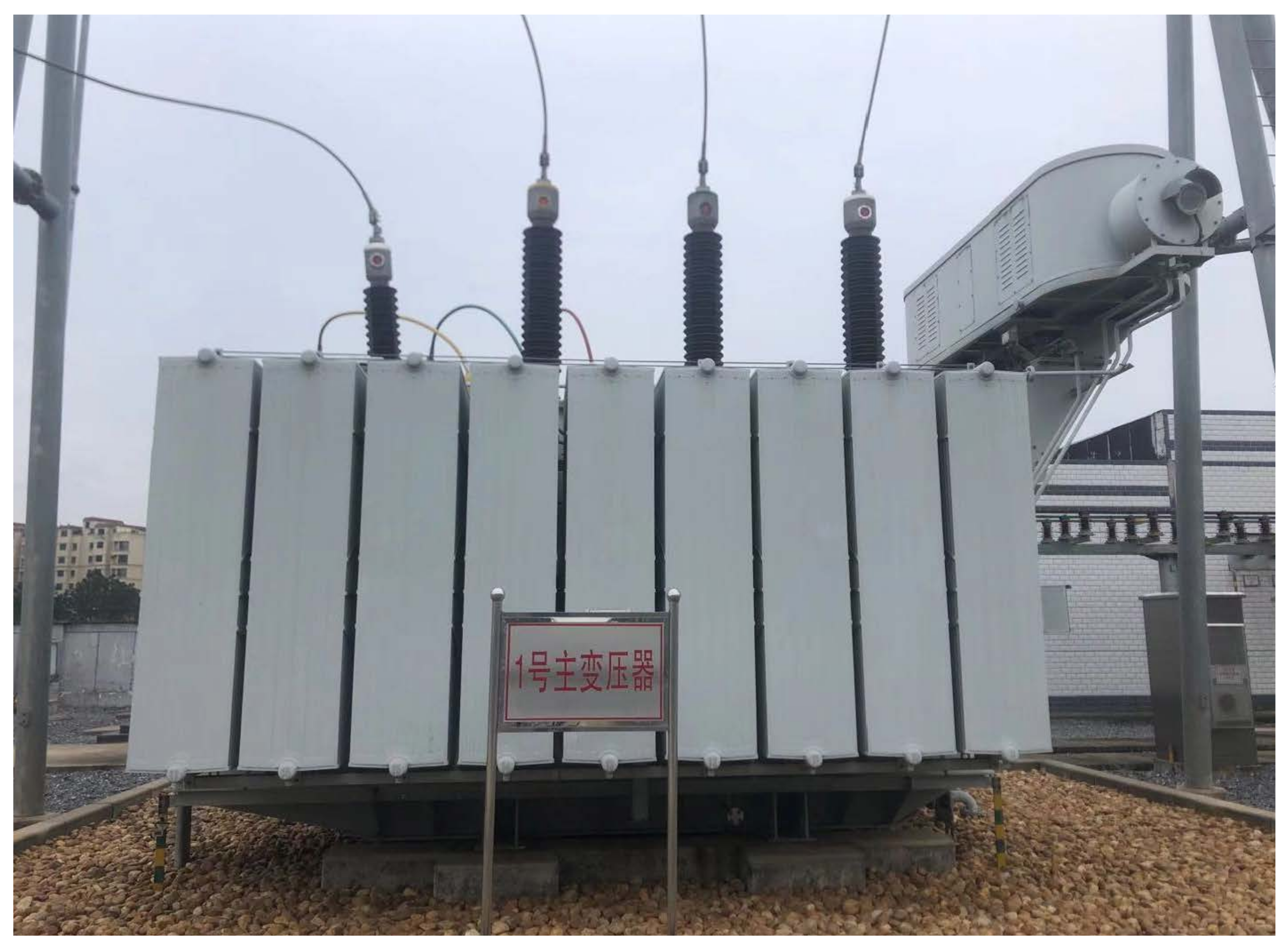
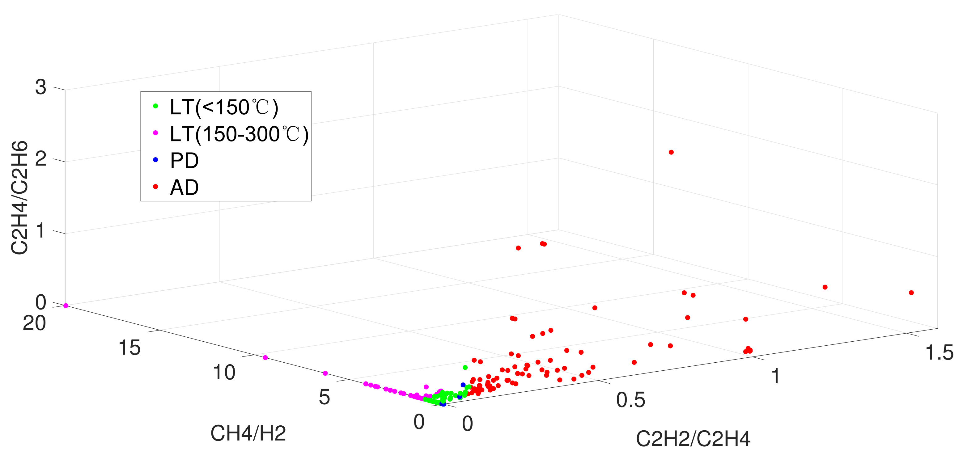
For a better test of the practical performance of the fault diagnosis model, it is necessary to consider the influence of the transformer capacity, ambient temperature and humidity, and other actual operating transformers itself and external conditions. Therefore, in this paper, the volume fractions of dissolved gases (CH, CH, CH, H, and CH) in oil of real power transformers were collected as sample data for the experiment using smart sensors at Jiangxi Power Company (PSC) in 2019. The normal operating temperature is 25 °C, and the set humidity is 50% [29]. The oil-immersed power transformer studied in this paper is shown in Figure 4. After eliminating some noisy and incomplete data, 555 sets of characteristic gas data of oil-immersed power transformers were obtained, including 361 sets of low temperature overheating (LT) (<150 °C), 40 sets of low temperature overheating (LT) (150–300 °C), 65 sets of partial discharge (PD), and 89 sets of arc discharge (AD).
After that, the data of 555 groups of characteristics were preprocessed by using three ratio method to reduce the dimensionality, and the ratios of characteristic gases (CH/CH, CH/H, and CH/CH) were used as fault characteristics, and some of the data after preprocessing are shown in Table 2. Figure 5 shows the distribution of all the data after the three-ratio method, and it can be seen that the ratios of characteristic gases data are too concentrated, especially the data with fault types LT and PD. In this case, it is difficult to obtain accurate and stable classification results with the artificially set diagnostic criteria such as IEC three-ratio method and Rogers’ method, and the superiority of neural network comes out for this unknown and complicated situation.
Later, 425 groups were filtered by randomly generated integer sequences as the training set and the remaining 130 groups as the test set. The divided data sets were imported into the input layer of the probabilistic neural network for training. Note that as the proposed fault diagnosis model is based on the classifier of the probabilistic neural network, the four fault types need to be re-coded and then input into the network, as shown in Table 3.
4. Experimental Results
4.1. Compared Methods
In order to demonstrate the effectiveness of the proposed method, we first compare IGWO-PNN with GWO-PNN and PNN and the traditional IEC three-ratio method (IEC) vertically; second, we conduct a cross-sectional comparison and select different metaheuristic algorithms combined with PNN to constitute different fault diagnosis models; and finally, use other more classical network models to compare with IGWO-PNN. The validity of the IGWO-PNN model is comprehensively demonstrated by comparing other more classical network models with IGWO-PNN.
For the above experimental objectives, three separate sets of comparison tests were set up.
The first group is a longitudinal comparison of IGWO-PNN, GWO-PNN, and PNN. In the second group, we selected several meta-heuristic algorithms proposed in the last 5 years to model fault diagnosis in combination with PNN: the Whale optimization algorithm (WOA)-PNN [30], Multi-Verse Optimizer (MVO)-PNN [31], Salp Swarm Algorithm (SSA)-PNN [32], and Seagull optimization algorithm (SOA)-PNN [33]. In the second group, we select some proposed and relatively traditional network models for comparison, namely, Bat Algorithm (BA)-BP [34], Cuckoo Search (CS)-BP [35], and Backpropagation Neural Network optimized by Particle swarm optimization and Genetic algorithm. We also introduce the Extreme learning machine (ELM), a more novel network compared to PNN and BP, as a control.
4.2. Results of Model Comparison
In this paper, the simulation platform Matlab 2018a is used to simulate the experiment. The calculation platform used in the experiment is i7-9750 CPU @ 2.60 GHz. The divided data set is imported into the input layer of PNN for training. The feature data processed by the three-ratio method is three-dimensional, so the network input layer is three layers, and the output layer is the fault classification layer. The number of layers is the same as the number of fault types, that is, the output layer is four layers.
Simulation experiments are performed according to the method proposed in Section 3.1. The parameters of each model in the simulation experiments are shown in Table 4.
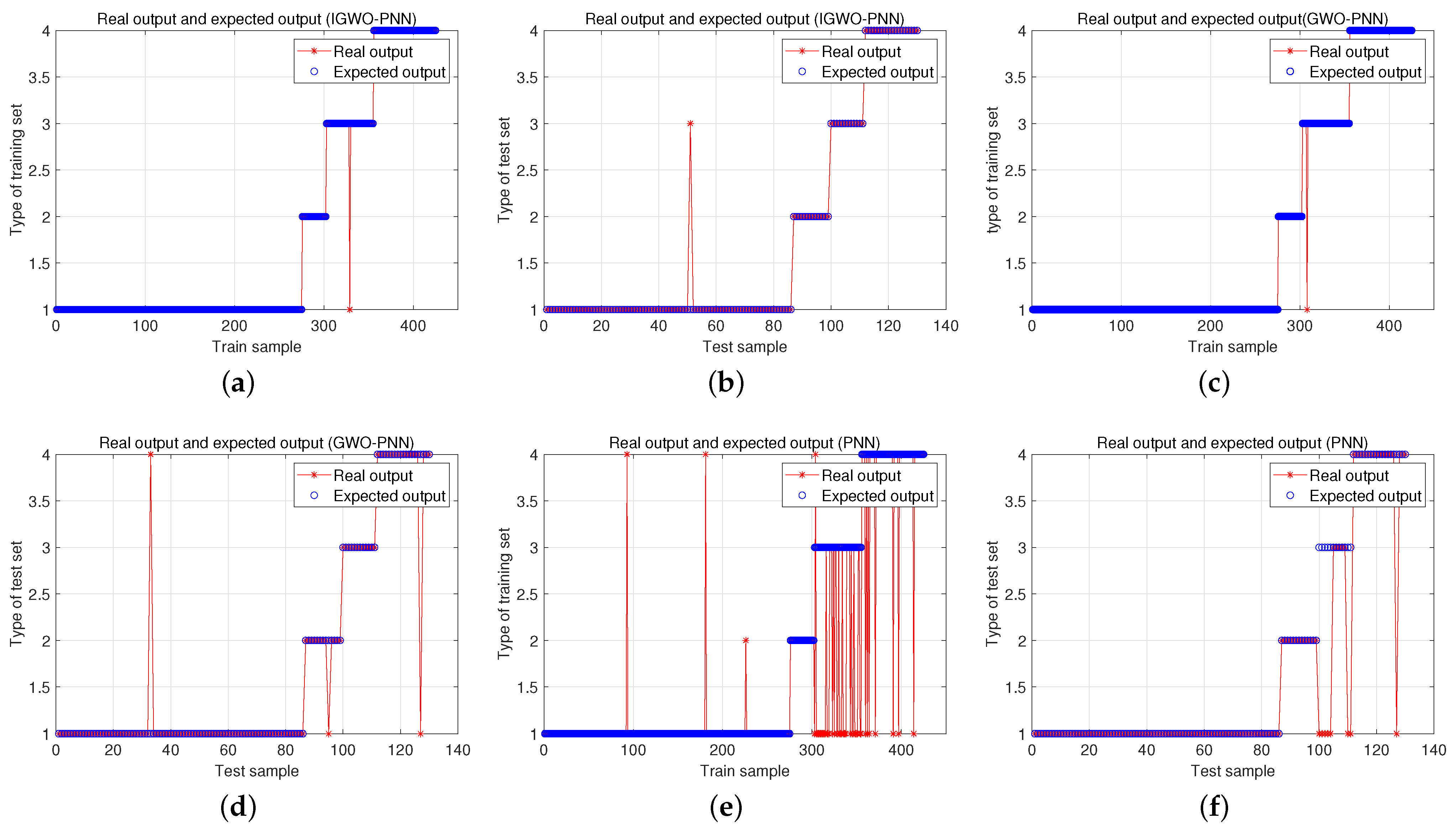
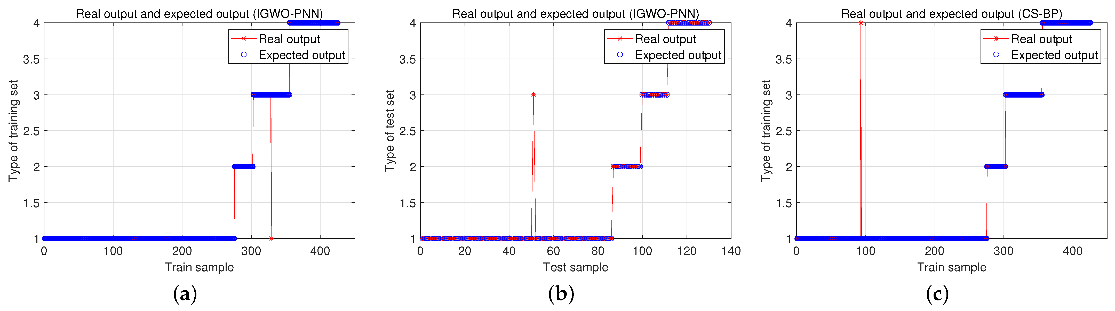
After the completion of the first set of comparison experiments, the results of each fault and the average accuracy are shown in Table 5. It can be seen that the average accuracy of IGWO-PNN on the test set is 99.71%, which is higher than that of GWO-PNN and PNN, and thus much higher than that of the traditional IEC three-ratio method, which fully reflects the superiority of the machine learning method compared with the traditional IEC three-ratio method. The diagnostic results of the three groups of machine learning models for the fault data samples in the table are shown in Figure 6, where Figure 6a,c,e shows the classification results of the training samples and Figure 6b,d,f shows the classification results of the test samples. From Figure 6, we can clearly see that the IGWO-PNN model performs the best among the three machine learning models in both the training and test sets. Furthermore, we can observe that the diagnostic results of PNN, both in the training and test sets, are far from GWO-PNN or IGWO-PNN. It is much larger than the difference between GWO-PNN and IGWO-PNN. Therefore, it can be demonstrated that the optimization of the smoothing factor by the metaheuristic algorithm can substantially improve the classification accuracy of PNN when used as a classifier.
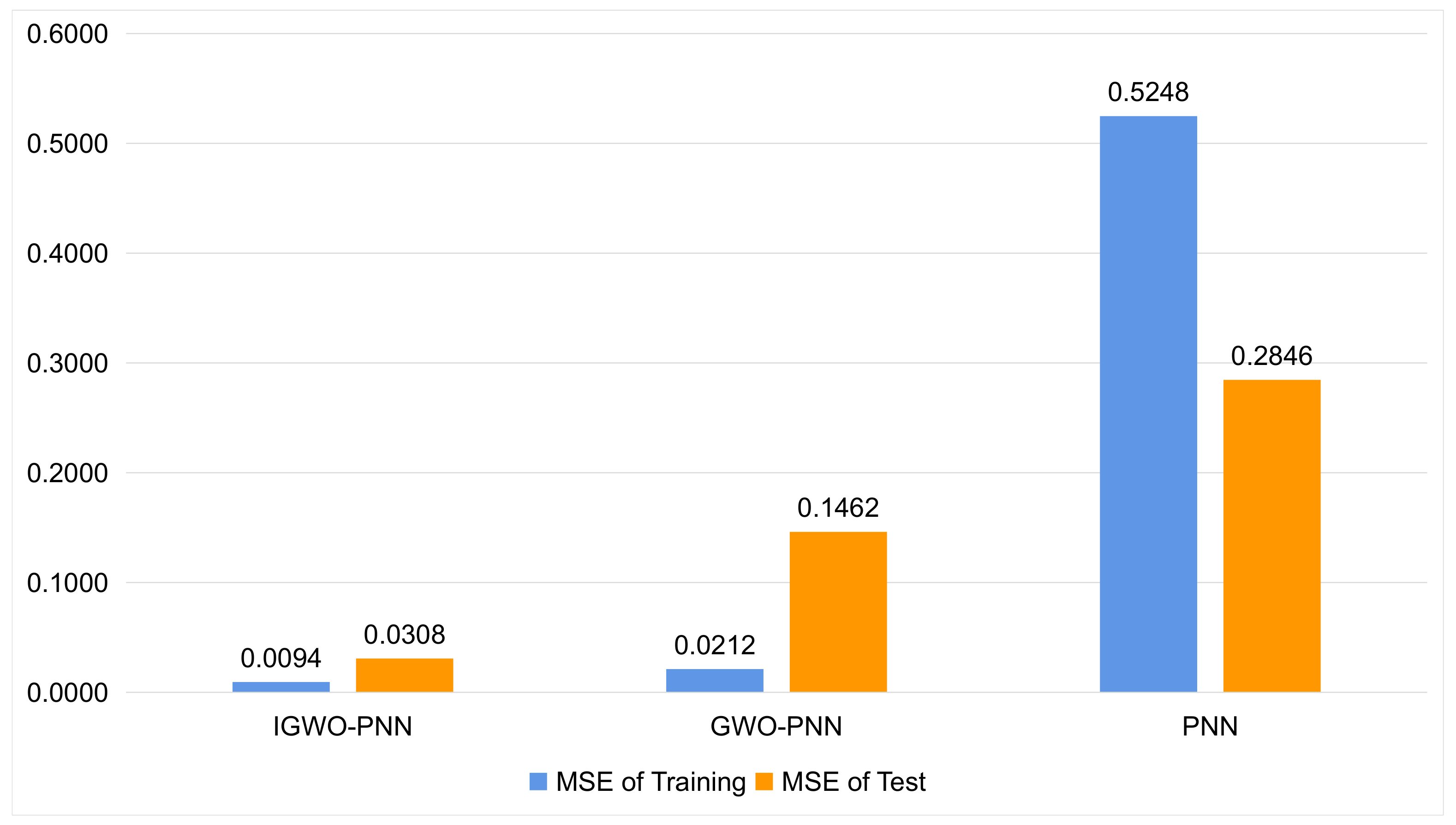
In order to demonstrate the superiority of the proposed method from several perspectives, we introduced the mean square error (MSE) in all three sets of comparison experiments. The MSEs of PNN, GWO-PNN, and IGWO-PNN in the first set of comparison experiments are shown in Figure 7.
It can be seen that the dispersion of IGWO-PNN is smaller and the stability of the model is stronger compared to PNN and GWO-PNN.
The feasibility and effectiveness of the optimization work of the smoothing factor and the improved theory of the GWO algorithm are fully demonstrated by the first set of experiments. The GWO algorithm was introduced in 2014, and many novel meta-heuristics have appeared since then. Does the improved GWO still have some superiority in the field of transformer fault diagnosis compared to these latecomers? This is the question that needs to be investigated in the second set of comparison experiments.
Again, based on the same training and test sets, the IGWO-PNN fault diagnosis model is compared with PNN fault diagnosis models composed of other novel intelligent algorithms in various aspects.
The results for each fault and the average accuracy are shown in Table 6.
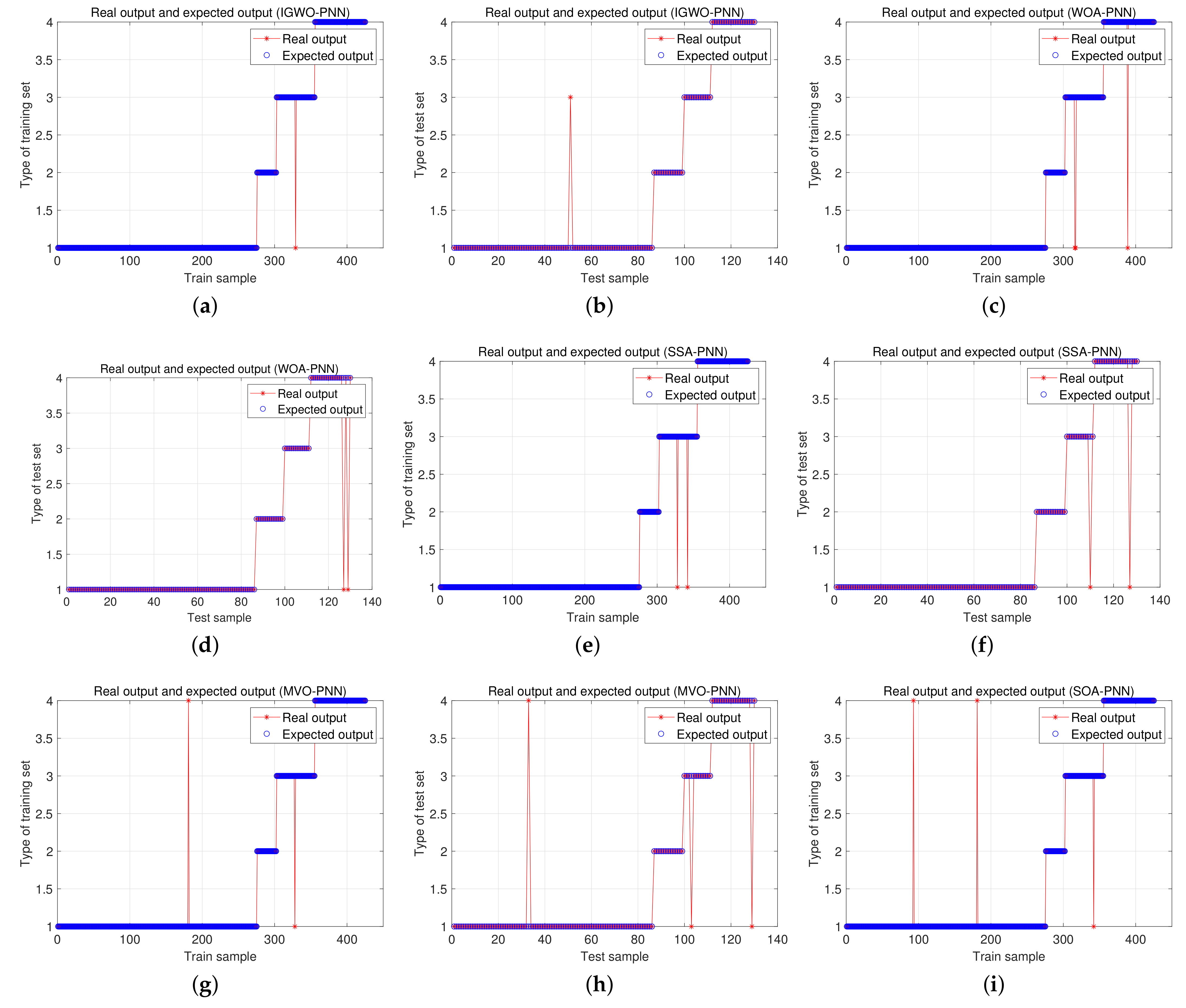
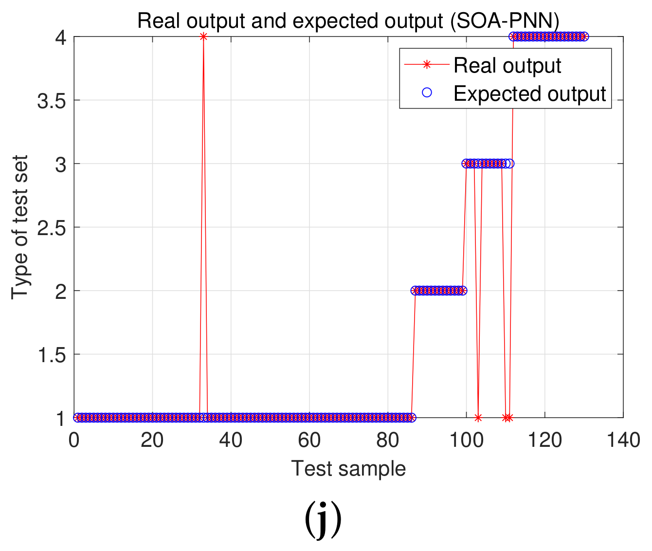
As can be seen from Table 6, the novel meta-heuristic algorithms are generally better at correcting the smoothing factors and generally have higher average precision on the test set. However, the average accuracy of IGWO-PNN is at least 2% higher than the average accuracy of other PNN models. It can be seen that based on the same fault data samples, IGWO still has some superiority over newer intelligent algorithms such as MVO, SSA, etc. Figure 8 shows the diagnostic results of the PNN fault diagnosis model of the novel metaheuristic algorithm in Table 6 based on the test set and the training set. IGWO-PNN has only one diagnostic failure, which is the best performance among all PNN models.
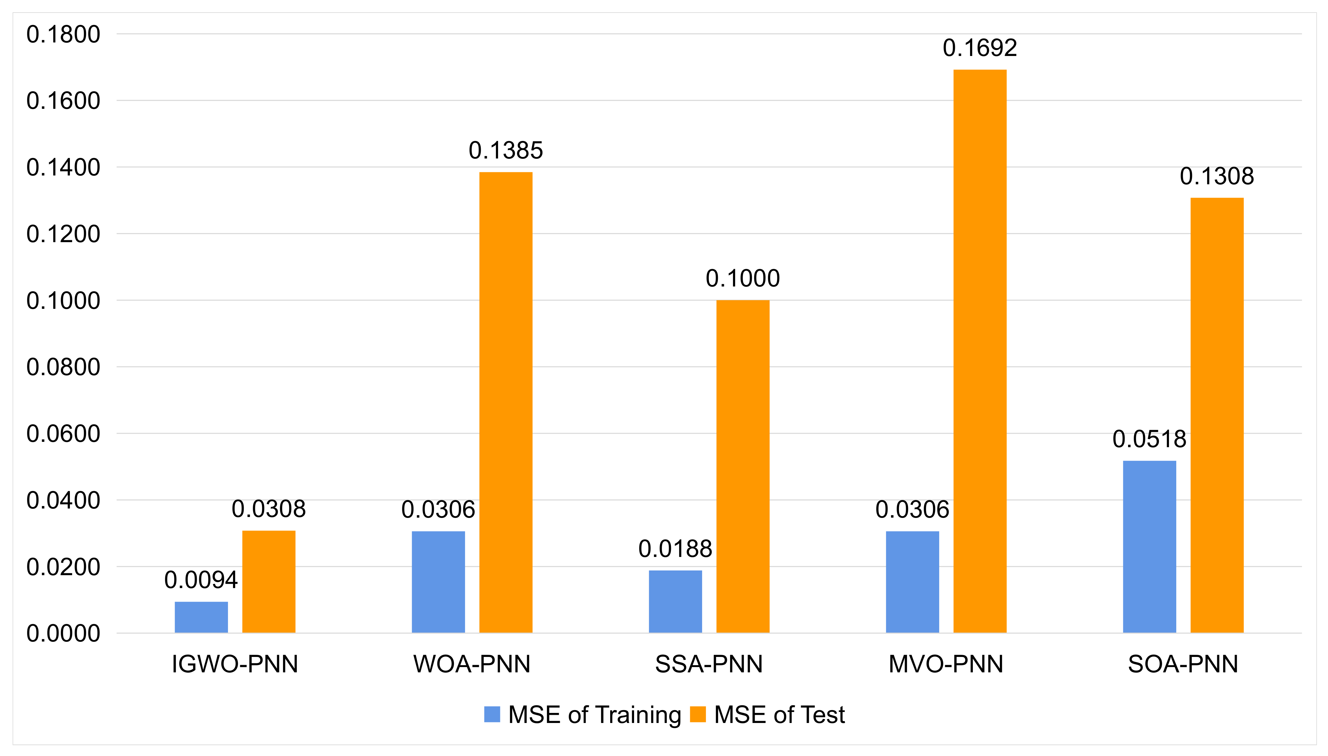
Similarly, we evaluate the five meta-heuristic algorithm models using MSE. The results are shown in Figure 9. The performance of several models in terms of MSE is more indicative of the usefulness of the models than comparing the average diagnostic accuracy. As seen in Figure 9, the MSEs of the other four meta-heuristic algorithms are greater than IGWO-PNN, both based on the training and test sets. The accuracy of the MVO-PNN model closest to IGWO-PNN is also three times more accurate than the MSE of IGWO-PNN.
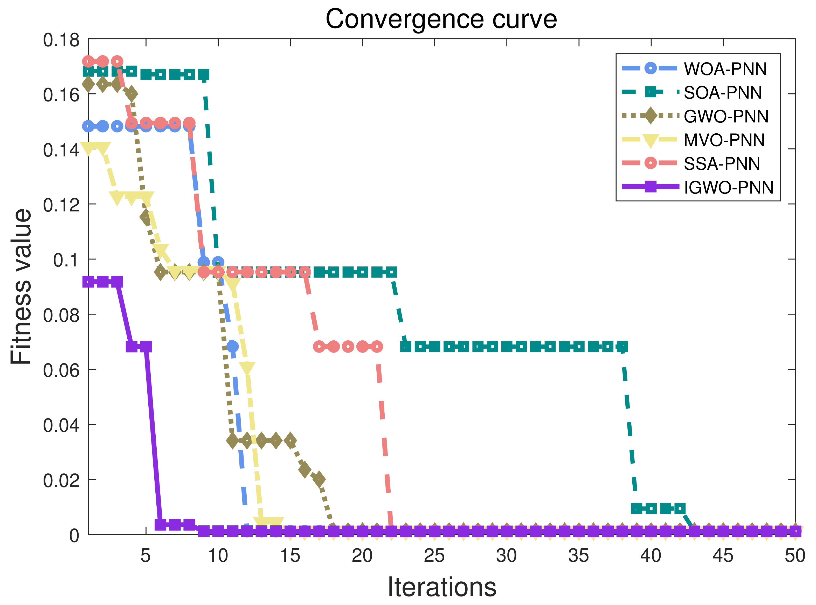
In order to demonstrate that the established IGWO-PNN model has a strong convergence capability for the faulty dataset, in the second set of comparison experiments, we introduce the fitness curves to demonstrate the merit-seeking process of each of the above-proposed six metaheuristics (including GWO), and the results are shown in Figure 10. As for IGWO, its fitness value starts decreasing from the third iteration and converges to the minimum fitness value at the ninth time. The whole process is within 10 iterations, which is the fastest among the six meta-heuristic algorithms. Compared with other algorithms, it is easier to jump out of the local optimum. This is enough to prove that the proposed update strategy has a significant improvement in the convergence ability of GWO.
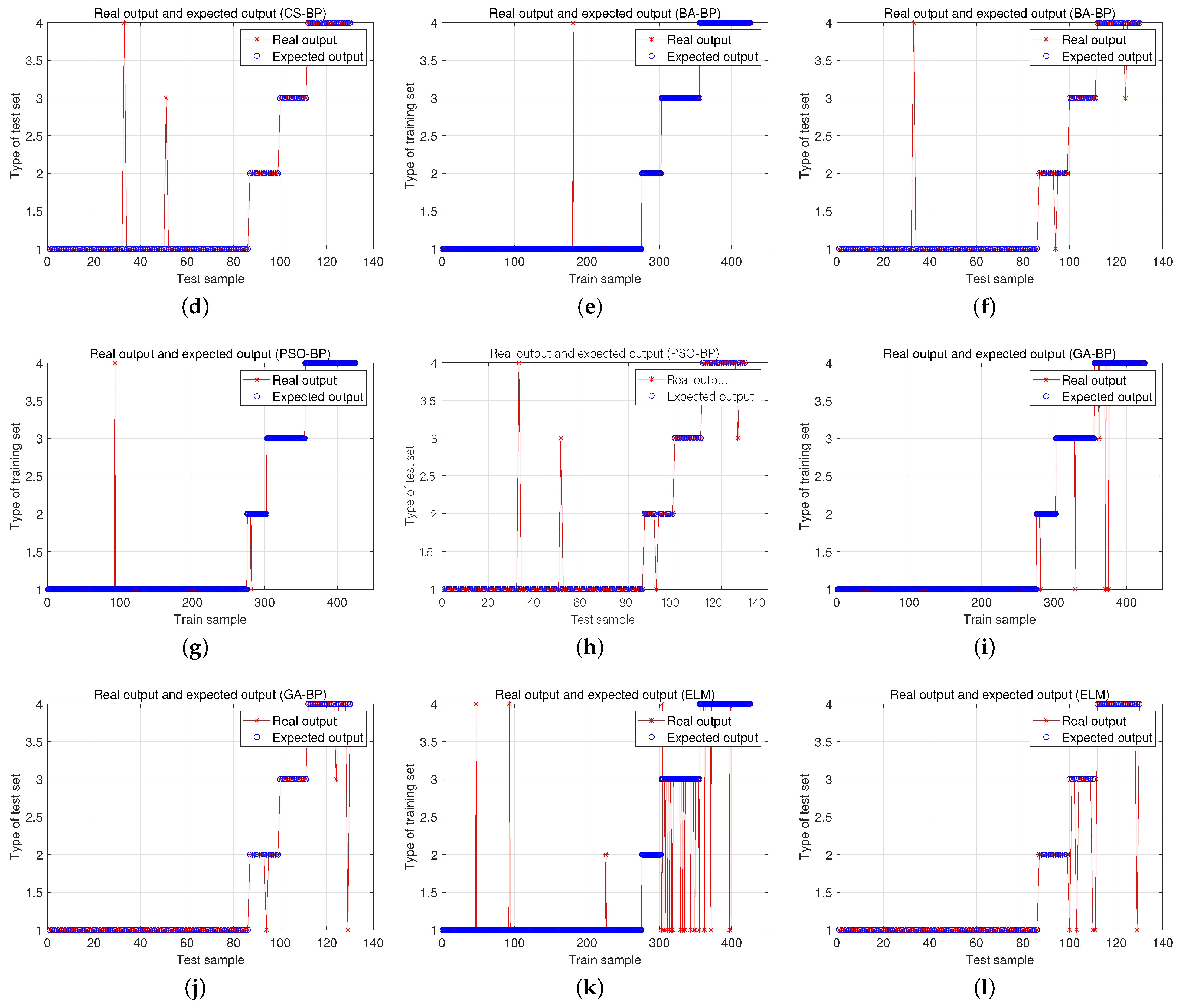
The first two sets of comparison experiments are discussed around PNN, and in the third set of comparison experiments, we choose other neural network models that have been proposed in the literature or are more classical (BP and ELM) to compare with the IGWO-PNN model. The results for each fault and the average accuracy are shown in Table 7, and Figure 11 shows the corresponding simulation results.
From the simulation results of the third set of comparison experiments, the IGWO-PNN model still has the highest diagnostic accuracy. However, the fault diagnosis models that have been proposed in other literature, such as CS-BP as well as BA-BP, are close to IGWO-PNN in terms of accuracy, especially CS-BP, which has an average accuracy of 99.42%. It can be seen that in terms of average accuracy, IGWO-PNN does not have much advantage.
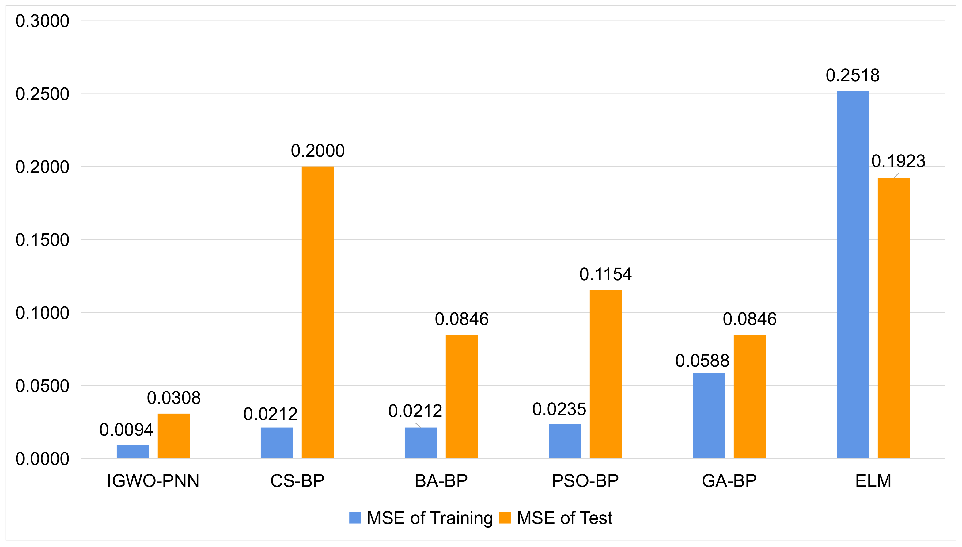
However, it can be seen by the MSEs of the six models shown in Figure 12. Although CS-BP is very close to IGWO-PNN in terms of average accuracy, its performance in terms of MSE is not optimistic compared to IGWO-PNN. In contrast, the stability and practicality of the newly proposed IGWO-PNN model are much better.
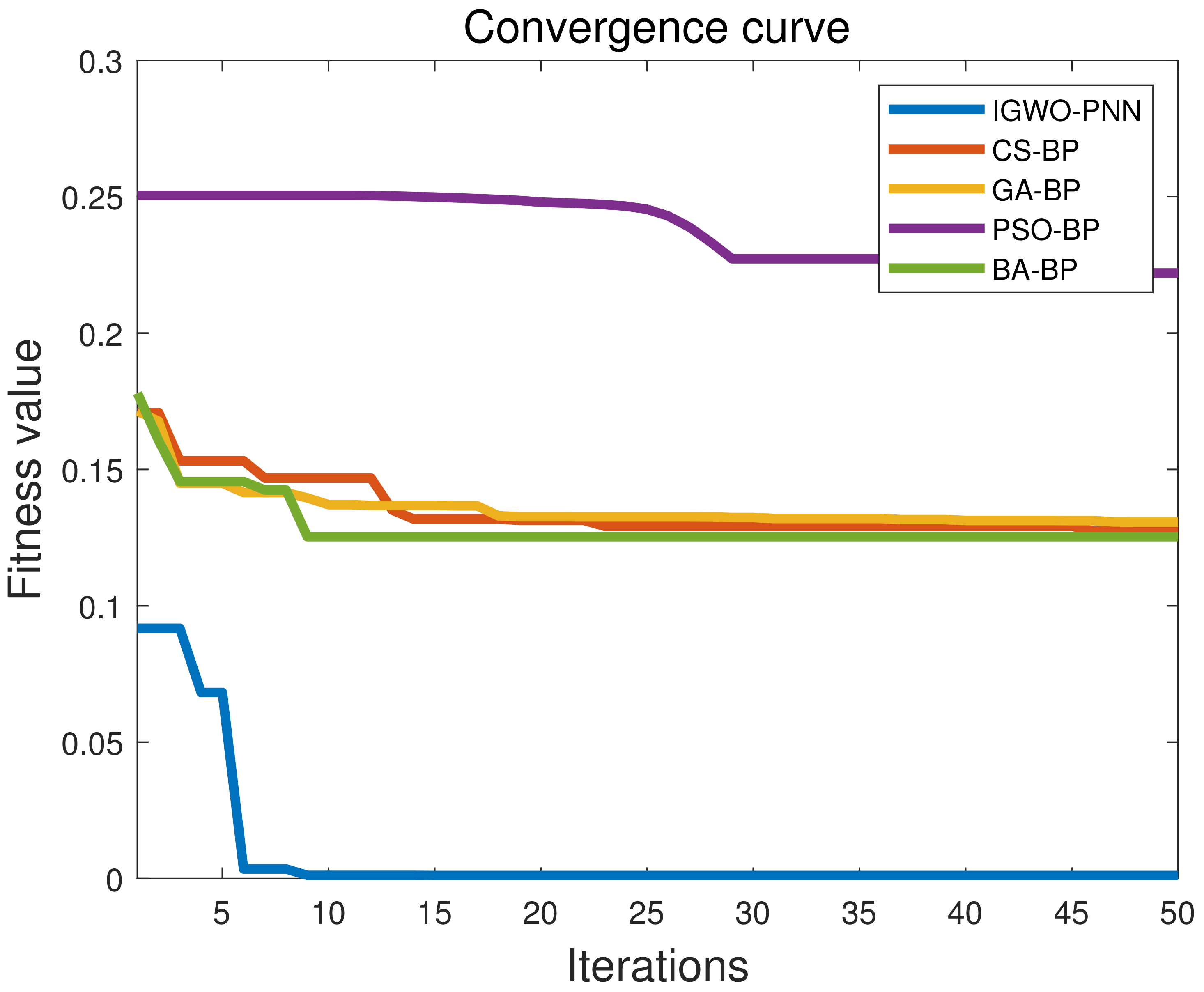
Similar to the second set of comparison experiments, we continue to introduce the fitness curves to observe the optimization search process of IGWO-PNN and the other four BP models. Note that among these four BP models, intelligent algorithms such as CS, BA, and PSO optimize the weights and bias of the BP neural network. The fitness curve is shown in Figure 13, which fully reflects the strong convergence ability of IGWO compared with the traditional metaheuristics such as CS, PSO, and BA. In this paper, the fitness function is MSE. From Figure 13, the fitness value of IGWO-PNN is much smaller than the other four models when it reaches the optimum within the maximum number of iterations, which again highlights the global search ability and stability of the IGWO model.
Considering the unbalanced nature of the collected fault data (low temperature overheating has much more data than several other types of faults), we chose to evaluate our classification model using the Marco F1-score. Table 8 shows the results of the Marco F1-score comparison for all the methods mentioned in this paper.
Accuracy is not a perfect metric for unbalanced datasets, and in this case, the F1-score better reflects the true performance of the classification model. Table 8 shows that when evaluating two different models, the model with relatively higher accuracy does not necessarily have a higher Marco F1-score than its rivals, such as the comparison between CS-BP and WOA-PNN. However, among all the models, the IGWO-PNN model still tops the list, which shows that the proposed model has a high classification utility.
The above three sets of comparison experiments show the superiority of the IGWO-PNN fault diagnosis model in terms of classification average accuracy, MSE, and diagnosis efficiency. However, up to the end, our experiments are based on the same set of training and test sets. To avoid the chance associated with using only one set of data, Table 9 shows the cross-validation results of different machine learning models.
The average accuracy obtained from the 5-fold, 10-fold, and 15-fold cross-validation results are clearly more convincing than the results obtained on the test set alone. The accuracy of the CS-BP model falls by as much as 4% compared to the test set, which shows that the results on the test set alone are somewhat chance. The average accuracy of the IGWO-PNN is 97.28%, which is the highest among all models, showing that the proposed model has good generalization ability. Although the results are slightly lower compared to those on the test set, this result better reflects the realistic performance of the model.
5. Conclusions
In this paper, a PNN fault diagnosis model combined with the IEC three-ratio method is proposed, and the standard update mechanism of GWO is modified and a DLH search mechanism is added. The improved method effectively improves the exploration ability and convergence ability of GWO. The improved GWO is used to optimize the smoothing factor of the PNN network, which improves the classification accuracy and robustness of the fault diagnosis model. The data used in this article come from the real transformer data of Jiangxi Power Supply Company, which is collected by smart sensors. Based on the same data, three sets of comparative experiments were carried out, involving a total of 13 diagnostic methods. Through the demonstration of three groups of comparative experiments and the reliability analysis of the experimental results, it can be seen that IGWO-PNN model has high engineering practicability in processing oil-immersed transformer fault data. Compared with other fault diagnosis models, its diagnosis accuracy and stability are outstanding.
Author Contributions
Conceptualization, X.Y. and Y.Z.; methodology, Y.Z.; software, L.T.; validation, Y.Z., L.T. and X.Y.; formal analysis, L.Y.; investigation, Y.Z.; resources, X.Y.; writing—original draft preparation, Y.Z., L.T.; writing—review and editing, Y.Z., L.T. and X.Y.; visualization, Y.Z.; supervision, X.Y. All authors have read and agreed to the published version of the manuscript.
Funding
This work was supported in part by the National Natural Science Foundation of China (51765042, 61963026).
Institutional Review Board Statement
Not applicable.
Informed Consent Statement
Not applicable.
Data Availability Statement
Not applicable.
Conflicts of Interest
There are no conflict from all authors of this paper.
References
- Wang, X.; Li, Q.; Li, C.; Yang, R.; Su, Q. Reliability assessment of the fault diagnosis methodologies for transformers and a new diagnostic scheme based on fault info integration. IEEE Trans. Dielectr. Electr. Insul. 2013, 20, 2292–2298. [Google Scholar] [CrossRef]
- Etumi, A.A.; Anayi, F. The application of correlation technique in detecting internal and external faults in three-phase transformer and saturation of current transformer. IEEE Trans. Power Deliv. 2016, 31, 2131–2139. [Google Scholar] [CrossRef]
- Oliveira, L.M.; Cardoso, A.M. A permeance-based transformer model and its application to winding interturn arcing fault studies. IEEE Trans. Power Deliv. 2010, 25, 1589–1598. [Google Scholar] [CrossRef]
- Pei, X.; Nie, S.; Chen, Y.; Kang, Y. Open-circuit fault diagnosis and fault-tolerant strategies for full-bridge DC–DC converters. IEEE Trans. Power Electron. 2011, 27, 2550–2565. [Google Scholar] [CrossRef]
- Faiz, J.; Soleimani, M. Assessment of computational intelligence and conventional dissolved gas analysis methods for transformer fault diagnosis. IEEE Trans. Dielectr. Electr. Insul. 2018, 25, 1798–1806. [Google Scholar] [CrossRef]
- Duval, M. The duval triangle for load tap changers, non-mineral oils and low temperature faults in transformers. IEEE Electr. Insul. Mag. 2008, 24, 22–29. [Google Scholar] [CrossRef]
- Arakelian, V. Effective diagnostics for oil-filled equipment. IEEE Electr. Insul. Mag. 2002, 18, 26–38. [Google Scholar] [CrossRef]
- Duval, M. New techniques for dissolved gas-in-oil analysis. IEEE Electr. Insul. Mag. 2003, 19, 6–15. [Google Scholar] [CrossRef]
- Khan, S.A.; Equbal, M.D.; Islam, T. A comprehensive comparative study of DGA based transformer fault diagnosis using fuzzy logic and ANFIS models. IEEE Trans. Dielectr. Electr. Insul. 2015, 22, 590–596. [Google Scholar] [CrossRef]
- Li, L.; Yong, C.; Long-Jun, X.; Li-Qiu, J.; Ning, M.; Ming, L. An integrated method of set pair analysis and association rule for fault diagnosis of power transformers. IEEE Trans. Dielectr. Electr. Insul. 2015, 22, 2368–2378. [Google Scholar] [CrossRef]
- Jiang, J.; Chen, R.; Chen, M.; Wang, W.; Zhang, C. Dynamic fault prediction of power transformers based on hidden Markov model of dissolved gases analysis. IEEE Trans. Power Deliv. 2019, 34, 1393–1400. [Google Scholar] [CrossRef]
- Li, J.; Zhang, Q.; Wang, K.; Wang, J.; Zhou, T.; Zhang, Y. Optimal dissolved gas ratios selected by genetic algorithm for power transformer fault diagnosis based on support vector machine. IEEE Trans. Dielectr. Electr. Insul. 2016, 23, 1198–1206. [Google Scholar] [CrossRef]
- Wang, X.; Li, Q.; Yang, R.; Li, C.; Zhang, Y. Diagnosis of solid insulation deterioration for power transformers with dissolved gas analysis-based time series correlation. IET Sci. Meas. Technol. 2015, 9, 393–399. [Google Scholar] [CrossRef]
- Chine, W.; Mellit, A.; Lughi, V.; Malek, A.; Sulligoi, G.; Pavan, A.M. A novel fault diagnosis technique for photovoltaic systems based on artificial neural networks. Renew. Energy 2016, 90, 501–512. [Google Scholar] [CrossRef]
- Li, S.; Wu, G.; Gao, B.; Hao, C.; Xin, D.; Yin, X. Interpretation of DGA for transformer fault diagnosis with complementary SaE-ELM and arctangent transform. IEEE Trans. Dielectr. Electr. Insul. 2016, 23, 586–595. [Google Scholar] [CrossRef]
- Dong, H.; Yang, X.; Li, A.; Xie, Z.; Zuo, Y. Bio-inspired PHM model for diagnostics of faults in power transformers using dissolved Gas-in-Oil data. Sensors 2019, 19, 845. [Google Scholar] [CrossRef]
- Kim, S.; Jo, S.H.; Kim, W.; Park, J.; Jeong, J.; Han, Y.; Kim, D.; Youn, B.D. A Semi-Supervised Autoencoder With an Auxiliary Task (SAAT) for Power Transformer Fault Diagnosis Using Dissolved Gas Analysis. IEEE Access 2020, 8, 178295–178310. [Google Scholar] [CrossRef]
- Song, T.; Jamshidi, M.M.; Lee, R.R.; Huang, M. A modified probabilistic neural network for partial volume segmentation in brain MR image. IEEE Trans. Neural Netw. 2007, 18, 1424–1432. [Google Scholar] [CrossRef]
- Kusy, M.; Zajdel, R. Probabilistic neural network training procedure based on Q (0)-learning algorithm in medical data classification. Appl. Intell. 2014, 41, 837–854. [Google Scholar] [CrossRef]
- Lee, J.H.; Kim, J.W.; Song, J.Y.; Kim, Y.J.; Jung, S.Y. A novel memetic algorithm using modified particle swarm optimization and mesh adaptive direct search for PMSM design. IEEE Trans. Magn. 2015, 52, 1–4. [Google Scholar] [CrossRef]
- Choi, K.; Jang, D.H.; Kang, S.I.; Lee, J.H.; Chung, T.K.; Kim, H.S. Hybrid algorithm combing genetic algorithm with evolution strategy for antenna design. IEEE Trans. Magn. 2015, 52, 1–4. [Google Scholar] [CrossRef]
- Li, X.; Ma, S.; Yang, G. Synthesis of difference patterns for monopulse antennas by an improved cuckoo search algorithm. IEEE Antennas Wirel. Propag. Lett. 2016, 16, 141–144. [Google Scholar] [CrossRef]
- Senthilnath, J.; Kulkarni, S.; Benediktsson, J.A.; Yang, X.S. A novel approach for multispectral satellite image classification based on the bat algorithm. IEEE Geosci. Remote Sens. Lett. 2016, 13, 599–603. [Google Scholar] [CrossRef]
- Yang, X.; Chen, W.; Li, A.; Yang, C.; Xie, Z.; Dong, H. BA-PNN-based methods for power transformer fault diagnosis. Adv. Eng. Inform. 2019, 39, 178–185. [Google Scholar]
- Mirjalili, S.; Mirjalili, S.M.; Lewis, A. Grey wolf optimizer. Adv. Eng. Softw. 2014, 69, 46–61. [Google Scholar] [CrossRef]
- Nadimi-Shahraki, M.H.; Taghian, S.; Mirjalili, S. An improved grey wolf optimizer for solving engineering problems. Expert Syst. Appl. 2021, 166, 113917. [Google Scholar] [CrossRef]
- Ma, J.; Li, Z.; Li, C.; Zhan, L.; Zhang, G.Z. Rolling Bearing Fault Diagnosis Based on Refined Composite Multi-Scale Approximate Entropy and Optimized Probabilistic Neural Network. Entropy 2021, 23, 259. [Google Scholar] [CrossRef]
- Specht, D.F. Probabilistic neural networks. Neural Netw. 1990, 3, 109–118. [Google Scholar] [CrossRef]
- Yang, X.; Chen, W.; Li, A.; Yang, C. A Hybrid machine-learning method for oil-immersed power transformer fault diagnosis. IEEJ Trans. Electr. Electron. Eng. 2020, 15, 501–507. [Google Scholar]
- Mirjalili, S.; Lewis, A. The whale optimization algorithm. Adv. Eng. Softw. 2016, 95, 51–67. [Google Scholar] [CrossRef]
- Mirjalili, S.; Mirjalili, S.M.; Hatamlou, A. Multi-verse optimizer: A nature-inspired algorithm for global optimization. Neural Comput. Appl. 2016, 27, 495–513. [Google Scholar] [CrossRef]
- Mirjalili, S.; Gandomi, A.H.; Mirjalili, S.Z.; Saremi, S.; Faris, H.; Mirjalili, S.M. Salp Swarm Algorithm: A bio-inspired optimizer for engineering design problems. Adv. Eng. Softw. 2017, 114, 163–191. [Google Scholar] [CrossRef]
- Dhiman, G.; Kumar, V. Seagull optimization algorithm: Theory and its applications for large-scale industrial engineering problems. Knowl. Based Syst. 2019, 165, 169–196. [Google Scholar] [CrossRef]
- Yang, X. A new metaheuristic bat-inspired algorithm. In Nature Inspired Cooperative Strategies for Optimization. (NICSO); Springer: Berlin/Heidelberg, Germany, 2011; Volume 284, p. 6574. [Google Scholar]
- Li, A.; Yang, X.; Dong, H.; Xie, Z.; Yang, C. Machine learning-based sensor data modeling methods for power transformer PHM. Sensors 2018, 18, 4430. [Google Scholar] [CrossRef]
Figure 1.
Probabilistic neural network structure diagram.

Figure 2.
Flow chart of IGWO-PNN.

Figure 3.
Power transformer fault diagnosis framework diagram.

Figure 4.
A power transformer with mineral oil as insulating material.

Figure 5.
Distribution of fault characteristic data.

Figure 6.
Comparison of the diagnosis results of the first set of comparative experiments. (a,c,e) represent the results of train sample classification for different methods, respectively. (b,d,f) are the results of testsample classification for different methods, respectively.
Figure 6.
Comparison of the diagnosis results of the first set of comparative experiments. (a,c,e) represent the results of train sample classification for different methods, respectively. (b,d,f) are the results of testsample classification for different methods, respectively.

Figure 7.
Comparison of the mean square error (MSE) of the first set of comparison experiments.

Figure 8.
Comparison of the diagnosis results of the second set of comparative experiments. (a,c,e,g,i) represent the results of train sample classification for different methods, respectively. (b,d,f,h,j) are the results of testsample classification for different methods, respectively.
Figure 8.
Comparison of the diagnosis results of the second set of comparative experiments. (a,c,e,g,i) represent the results of train sample classification for different methods, respectively. (b,d,f,h,j) are the results of testsample classification for different methods, respectively.


Figure 9.
Comparison of the MSE of the second set of comparison experiments.

Figure 10.
The fitness curve of different methods in the second set of comparative experiments.

Figure 11.
Comparison of the diagnosis results of the third set of comparative experiments. (a,c,e,g,i,k) represent the results of train sample classification for different methods, respectively. (b,d,f,h,j,l) are the results of testsample classification for different methods, respectively.
Figure 11.
Comparison of the diagnosis results of the third set of comparative experiments. (a,c,e,g,i,k) represent the results of train sample classification for different methods, respectively. (b,d,f,h,j,l) are the results of testsample classification for different methods, respectively.


Figure 12.
Comparison of the MSE of the third set of comparison experiments.

Figure 13.
The fitness curve of different methods in the third set of comparative experiments.


Table 1.
Fault diagnosis based on IEC three-ratio method.
| Fault Type | CH/CH | CH/H | CH/CH |
|---|---|---|---|
| LT (<150 °C) | <0.1 | 0.1 ∼ 1 | 1 ∼ 3 |
| LT (150–300 °C) | <0.1 | ≥1 | <1 |
| PD | <0.1 | <0.1 | <1 |
| AD | 0.1 ∼ 3 | <1 | NS |
NS: Non-significant whatever the value. LT (<150 °C): Low temperature overheating (LT) (<150 °C). LT (150–300 °C): Low temperature overheating (LT) (150–300 °C). PD: Partial discharge; AD: Arc discharge.
Table 2.
Some dissolved gas analysis data collected from actual transformers.
| Dissolved Gas, µL/L | Fault Type | ||
|---|---|---|---|
| CH/CH | CH/H | CH/CH | |
| 0.07143 | 0.54667 | 0.03571 | LT(<150 °C) |
| 0 | 0.17529 | 0 | LT(<150 °C) |
| 0.03846 | 0.8214 | 0.04348 | LT(<150 °C) |
| 0.01583 | 1.68618 | 0.00179 | LT(150–300 °C) |
| 0.01613 | 1.125 | 0.01389 | LT(150–300 °C) |
| 0.01667 | 1.08108 | 0.01563 | LT(150–300 °C) |
| 0.05556 | 0.07524 | 0.05882 | PD |
| 0 | 0.07059 | 0 | PD |
| 0.06667 | 0.06754 | 0.21910 | PD |
| 0.25 | 0.32323 | 0.33333 | AD |
| 0.14844 | 0.07836 | 0.14394 | AD |
| 0.125 | 0.13768 | 0.16667 | AD |
Table 3.
Coding format for four types of faults.
| Fault Type | LT (<150 °C) | LT (150–300 °C) | PD | AD |
|---|---|---|---|---|
| Coding format | 1 | 0 | 0 | 0 |
| 0 | 1 | 0 | 0 | |
| 0 | 0 | 1 | 0 | |
| 0 | 0 | 0 | 1 |
Table 4.
Parameter setting of various methods.
| Methods | Parameters Settings |
|---|---|
| PSO-BP | c1 = c2 = 1.49445, N = 10, T = 50 |
| IGWO-PNN | = 2, = 0, N = 10, T = 50 |
| SOA-PNN | N = 10, T = 50 |
| WOA-PNN | N = 10, T = 50 |
| MVO-PNN | Universes_no = 10, T = 50 |
| SSA-PNN | N = 10, T = 50 |
| GWO-PNN | a was linearly decreased from 2 to 0, N = 10, T = 50 |
| BA-BP | N = 10, T = 50, A = 0.5, r = 0.5 |
| CS-BP | N = 10, T = 50, Pa = 0.25 |
| GA-BP | N = 10, T = 50, Pm = 0.01, Px = 0.7 |
| ELM | HiddenNum = 20, TF = ‘sig’ |
| PNN | Spread = 0.07 |
Table 5.
Results of the first set of comparative experiments.
| Fault Type | Accuracy (%) | |||
|---|---|---|---|---|
| IGWO-PNN | GWO-PNN | PNN | IEC | |
| LT (<150 °C) | 98.84 | 98.84 | 100.00 | 0.28 |
| LT (150–300 °C) | 100.00 | 92.31 | 100.00 | 100.00 |
| PD | 100.00 | 100.00 | 41.67 | 100.00 |
| AD | 100.00 | 94.74 | 94.74 | 100.00 |
| Average | 99.71 | 96.47 | 84.10 | 75.07 |
Table 6.
Results of the second set of comparative experiments.
| Fault Type | Accuracy (%) | ||||
|---|---|---|---|---|---|
| IGWO-PNN | WOA-PNN | SSA-PNN | MVO-PNN | SOA-PNN | |
| LT (<150 °C) | 98.84 | 100.00 | 100.00 | 98.84 | 98.84 |
| LT (150–300 °C) | 100.00 | 100.00 | 100.00 | 100.00 | 100.00 |
| PD | 100.00 | 100.00 | 91.67 | 91.67 | 75.00 |
| AD | 100.00 | 89.47 | 94.74 | 94.74 | 100.00 |
| Average | 99.71 | 97.37 | 96.60 | 96.31 | 93.46 |
Table 7.
Results of the third set of comparative experiments.
| Fault Type | Accuracy (%) | |||||
|---|---|---|---|---|---|---|
| IGWO-PNN | CS-BP | BA-BP | PSO-BP | GA-BP | ELM | |
| LT (<150 °C) | 98.84 | 97.67 | 98.84 | 97.67 | 100.00 | 100.00 |
| LT (150–300 °C) | 100.00 | 100.00 | 92.31 | 92.31 | 92.31 | 100.00 |
| PD | 100.00 | 100.00 | 100.00 | 100.00 | 100.00 | 66.67 |
| AD | 100.00 | 100.00 | 94.74 | 94.74 | 89.47 | 94.74 |
| Average | 99.71 | 99.42 | 96.47 | 96.18 | 95.45 | 90.35 |
Table 8.
Marco FI-score of different methods.
| Methods | Marco F1-Score | ||||
|---|---|---|---|---|---|
| LT (<150 °C) | LT (150–300 °C) | PD | AD | Average | |
| IGWO-PNN | 99.42% | 100.00% | 96.30% | 100.00% | 98.93% |
| CS-BP | 98.82% | 100.00% | 92.31% | 97.44% | 97.14% |
| WOA-PNN | 98.88% | 100.00% | 100.00% | 94.44% | 98.33% |
| SSA-PNN | 98.88% | 100.00% | 95.65% | 97.30% | 97.96% |
| GWO-PNN | 98.31% | 96.00% | 100.00% | 95.00% | 97.33% |
| BA-BP | 98.85% | 96.00% | 96.30% | 95.00% | 96.54% |
| MVO-PNN | 98.31% | 100.00% | 95.65% | 95.00% | 97.24% |
| PSO-BP | 98.25% | 96.00% | 93.33% | 95.00% | 95.64% |
| GA-BP | 98.88% | 96.00% | 96.30% | 94.44% | 96.40% |
| SOA-PNN | 97.78% | 100.00% | 85.71% | 97.56% | 95.26% |
| ELM | 97.33% | 96.30% | 84.21% | 97.30% | 93.78% |
| PNN | 95.92% | 100.00% | 58.82% | 97.30% | 88.01% |
Table 9.
K-fold cross-validation results of different methods.
| Methods | K-Fold Cross-Validation | |||
|---|---|---|---|---|
| 5-Folds | 10-Fold | 15-Fold | Average | |
| IGWO-PNN | 98.76% | 96.11% | 96.97% | 97.28% |
| CS-BP | 95.88% | 95.94% | 93.25% | 95.02% |
| BA-BP | 93.15% | 94.32% | 89.61% | 92.36% |
| MVO-PNN | 95.60% | 92.91% | 87.85% | 92.12% |
| PSO-BP | 92.14% | 88.25% | 93.27% | 91.22% |
| SSA-PNN | 95.06% | 90.72% | 85.19% | 90.32% |
| SOA-PNN | 92.14% | 87.25% | 86.89% | 88.76% |
| GA-BP | 93.97% | 86.65% | 85.46% | 88.69% |
| GWO-PNN | 94.74% | 85.68% | 84.59% | 88.34% |
| WOA-PNN | 94.18% | 83.54% | 83.24% | 86.99% |
| ELM | 90.71% | 79.04% | 88.50% | 86.08% |
| PNN | 87.87% | 71.25% | 78.74% | 79.29% |
Publisher’s Note: MDPI stays neutral with regard to jurisdictional claims in published maps and institutional affiliations. |
© 2021 by the authors. Licensee MDPI, Basel, Switzerland. This article is an open access article distributed under the terms and conditions of the Creative Commons Attribution (CC BY) license (https://creativecommons.org/licenses/by/4.0/).
Share and Cite
MDPI and ACS Style
Zhou, Y.; Yang, X.; Tao, L.; Yang, L. Transformer Fault Diagnosis Model Based on Improved Gray Wolf Optimizer and Probabilistic Neural Network. Energies 2021, 14, 3029. https://0-doi-org.brum.beds.ac.uk/10.3390/en14113029
AMA Style
Zhou Y, Yang X, Tao L, Yang L. Transformer Fault Diagnosis Model Based on Improved Gray Wolf Optimizer and Probabilistic Neural Network. Energies. 2021; 14(11):3029. https://0-doi-org.brum.beds.ac.uk/10.3390/en14113029
Chicago/Turabian StyleZhou, Yichen, Xiaohui Yang, Lingyu Tao, and Li Yang. 2021. "Transformer Fault Diagnosis Model Based on Improved Gray Wolf Optimizer and Probabilistic Neural Network" Energies 14, no. 11: 3029. https://0-doi-org.brum.beds.ac.uk/10.3390/en14113029
Note that from the first issue of 2016, this journal uses article numbers instead of page numbers. See further details here.