Stratified Control Applied to a Three-Phase Unbalanced Low Voltage Distribution Grid in a Local Peer-to-Peer Energy Community

Abstract

This paper presents control relationships between the low voltage distribution grid and flexibilities in a peer-to-peer local energy community using a stratified control strategy. With the increase in a diverse set of distributed energy resources and the next generation of loads such as electric storage, vehicles and heat pumps, it is paramount to maintain them optimally to guarantee grid security and supply continuity. Local energy communities are being introduced and gaining traction in recent years to drive the local production, distribution, consumption and trading of energy. The control scheme presented in this paper involves a stratified controller with grid and flexibility layers. The grid controller consists of a three-phase unbalanced optimal power flow using the holomorphic embedding load flow method wrapped around a genetic algorithm and various flexibility controllers, using three-phase unbalanced model predictive control. The control scheme generates active and reactive power set-points at points of common couplings where flexibilities are connected. The grid controller’s optimal power flow can introduce additional grid support functionalities to further increase grid stability. Flexibility controllers are recommended to actively track the obtained set-points from the grid controller, to ensure system-level optimization. Blockchain enables this control scheme by providing appropriate data exchange between the layers. This scheme is applied to a real low voltage rural grid in Austria, and the result analysis is presented.

1. Introduction

In recent years, local energy communities (LECs) are gaining interest in Europe and the world by introducing new regulations for its formation, operation and control. LECs’ introduction is due to increased distributed renewable energy sources (DERs) and new loads such as electric vehicles, storage and heat pumps, hereafter referred to as next-gen loads, in low voltage distribution grids. This is to motivate the local generation, distribution, consumption and trading of energy. The research presented in this paper is conducted under the Blockchian Grid project funded by the Climate and Energy Fund and implemented in the RTI-initiative “Flagship region Energy” of the Austrian Research Promotion Agency. The most significant limitation of a local energy market associated within an LEC is the availability of a settlement process. Such processes are in place to ensure no violation occurs in the grid when the bids, accepted in the market, are executed. The need is due to the lack of controllability of DERs and next-gen-loads. In this context, a stratified control system, which manages both the grid and various DERs and flexibilities, could be one of the approaches.

In the literature, stratified control for flexibility management is extensively used. In [1], a stratified control scheme to control voltage and current is presented. It includes the optimal reconfiguration of various systems in micro-grid based on changing conditions. The first layer consists of the optimal sharing of load and the second level consists of dynamic optimization of droop gains. However, this approach is not designed for three phase systems as size of the problem will start to become large. Additionally, the second level consists of only droop gains where flexibilities, which offer on/off behavior cannot be included. The authors of [2] have proposed a hierarchical energy management system, to interconnect multiple micro-grids. At the higher level, micro-grid coordination operations are performed based on energy scheduling and generation of power reference values for other micro-grids.In the lower level, a chance-constrained MPC is applied for local operation management. The goal to maximize the local utilization of capacities and reduce the dependence on interconnected grids. A major limitation of this approach is that the higher level control does not include an optimal power flow based scheduling algorithm, leading to a sub-optimal solution. In [3], a hybrid stratified control to improve grid security is presented. In the lower level, the controllers are responsible for coordinating each of the individual control units. Whereas, in the higher level, continuous dynamic control of discrete controllers and with individual lower-level controllers is presented. The authors of [4] have presented a hierarchical iterative control algorithm to balance the grid optimally and, at the same time, meet consumer demand. The major limitation of the control strategies mentioned above is the need for detailed technical models of lower-level controllers. Detailed models are often not available or difficult to derive, making them unrealistic for implementation. Additionally, any change in the devices at the lower level needs to be recorded and appropriate adjustment in the algorithm needs to be made. However, in this paper, optimal schedules are generated at the PCC of flexibilities irrespective of what is connected to it. Moreover, the data exchange between each layer and within each layer needs to be sufficiently strong enough to handle a large number of variables being exchanged. Blockchain with a 15s block speed is used in this paper to write data into the chain, which is available in all other buses in the next sample.

The stratified controller consists of an OPF at the upper level. As discussed in [5], OPF algorithms can be classified into two types, A and B, respectively. Type A deals with algorithms that use load flow methods to generate a certain set of intermediate solutions for voltages and phase angles. Since the optimal solution is close to the load flow solution, using jacobian and other sensitivity relations, it can be sequentially determined. Various implementations of class A algorithms are presented in [6,7,8]. Class B deals with algorithms that use load flow equations as equality constraints, depending on the exact conditions and detailed formulation. It utilizes the entire search space. Since power grids are nonlinear and non-convex in nature, convex relaxation or non-convex solvers are to be used. It uses optimality conditions using Lagrangian functions with objective and constraint derivatives. In [9], a novel class C algorithm is presented in which a reliable load flow is coupled with a heuristic optimization method. This method helps to overcome the challenges presented by classes A and B, which are used in this paper.

Low voltage rural distribution grids are unbalanced due to untransposed lines and uneven loading on their three-phases [10]. The unbalance can be heightened with increase in single-phase DERs and next-gen loads [11,12]. They are dependent on weather parameters such as temperature and solar irradiation. Moreover, they are periodic, with hourly, daily, weekly and monthly cycles and are dependent on seasons. Three-phase unbalance, induces several issues in the grid. Most prominently, it increases losses in lines, grid devices and transformers. Transformers in the distribution grids are designed for balanced operation and would lead to uneven temperatures on the three phases, causing degradation [13]. Induction motors are significantly affected by voltage imbalance, causing accelerated aging due to high temperatures on winding with the highest loading and shorten the lifespan [14]. Torque fracturing can lead to permanent damage in motor winding with the increase in voltage unbalance [15]. Protection systems can be triggered falsely due to the presence of negative and zero sequence currents in the lines [16]. Currently, models describing the low voltage distribution grids are based on the transmission system’s supervisory control and data acquisition systems at the transmission level. This host functions like load (LF) and optimal power flow (OPF), using models that are single phased. They cannot be readily applied to distribution grids without modification to accommodate the new changes, as discussed above. To overcome this, the LF and OPF should include three-phase unbalance.

In the literature, various methods have been presented to minimize three-phase unbalance, which can be consolidated into three types. Namely, phase transposition, feeder reconfiguration, and power control. In [17], a method to minimize three-phase unbalance for both star and delta configurations is presented. This is performed by operating various devices connected to the IEEE 34 and 123 bus test systems. The grid is linearized to convert non-linearity non-convexity to mixed-integer linear programming. The authors of [18] have formulated a method to minimize three-phase unbalance by re-phasing and reconfiguration using optimization techniques and by optimally placing DER units. In [19], re-phasing and DER sizing are used to achieve three-phase unbalance minimization. A fuzzy multi-objective phase balancing optimization is used to do so. Various heuristic optimization techniques for three-phase unbalance minimization is presented in [16,20,21]. Various phase swapping algorithms are reviewed in [22]. In [23], power balance is used to minimize unbalance by optimally operating energy storage, and a similar method is presented in [24]. Various methods involving reactive power control for unbalance minimization are available in the literature. In [25], static variable compensators are used to balance the three phases. The authors of [26] describe a method to minimize zero and negative sequence current components in distribution grids. It involves the use of reactive power management using the online Karush–Kuhn–Tucker optimization method. This method is applied to IEEE 13-node test network. Most of the methods mentioned above are used in the planning phase. This does not include the dynamic behavior of unbalanced loads and generation. In this paper, the stratified controller is to minimize the three-phase voltage unbalance in real-time.

Flexibilities are controlled using model predictive control (MPC) and, in the literature, various implementations are available. In [27], a multi-time scale and stage optimization method is proposed to control flexibilities such as air conditioning, heating and ventilation systems, and plug-in hybrid electric vehicles are presented. It uses a constrained stochastic optimization algorithm using MPC to minimize costs, peak power and consumer comfort. Temperature data, thermal dynamics and real-time electricity pricing are included. The authors of [28] have presented an MPC approach to shifting loads among household devices and electric storage systems. Energy consumption is minimized by using time of day tariff and demand-side management (DSM) by optimally scheduling loads and charging and discharging times of the electric storage system. An appliance scheduling method in residential buildings using MPC is presented in [29]. It involves the use of thermal and non-thermal flexibilities by incorporating forecasts and database updates to minimize electricity costs. It includes a thermal dynamic of the building and is used as constraints to MPC. In [30], the MPC approach to controlling photo-voltaic combined heat and electric storage is presented. The operational cost of the combined heat and power unit is minimized. The authors of [31] have presented a method to control the air conditioning system in the room, along with the PV system. Demand response is provided using time of use tariff. Additionally, the controller is used to minimize energy consumption. In [32], the authors present a three-phase unbalanced model predictive control based smart building energy management system. It uses three-phase flexibility models with mixed-integer quadratic programming. In this paper, the smart building models and control strategies are derived from it.

To overcome the limitations presented in the literature, the authors present a novel stratified control scheme with grid and flexibility layers. The former consists of three-phase unbalanced optimal power flow using the holomorphic embedding load flow method (HELM) and the latter, three-phase unbalanced model predictive control. Blockchain handles all exchanges of control variables (see Section 2). The flexibilities are connected at a certain number of buses which are considered controllable, and the grid level controller generates three-phase optimal active (P) and reactive power (Q) schedules at their points of common couplings (PCC). The grid level controller concentrates PQ consumption and in-feed values from smart meters, from all other uncontrollable loads in the LEC over the Blockchain for each sample time. Contrary to the methods presented in the literature, the grid level controller does not contain any information about the devices connected at the PCC, ensuring individual privacy. The stratified controller uses models that include three-phase controls for both PQ flows, resulting in per-phase power manipulation. These schedules are actively tracked by the flexibilities along with their objectives, leading to a system-level optimization. The grid level controller uses Optimal Power Flow (OPF), based on a three-phase unbalanced holomorphic embedding load flow method (HELM) and genetic algorithm with certain advantages over the existing methods (see Section 4). As discussed above, the DERs and next-gen loads are intermittent, dependent on external factors and, therefore, model predictive control (MPC) (see Section 5), with its proven robustness, is used to manage them optimally.

The contributions in this paper are listed below:

1

Stratified control structure for optimal scheduling of grid flexibility in an LEC using Blockchain (see Section 3 and Section 6).

2

Online three-phase unbalance minimization control scheme in low voltage distribution networks (see Section 4.1.1) in an LEC.

3

Three-phase unbalance optimal power flow with receding horizon formulation for optimal flexibility placement (see Section 4.1.2) and voltage controllability (see Section 4.1.3 and Section 6).

4

Schedules from the grid controller are generated at the PCC, ensuring privacy. No device information from the buildings is communicated to the grid controller.

5

Mixed integer quadratic three-phase unbalanced model predictive control hosted in flexibilities with various electrical connection configurations and thermal models (see Section 5.1).

6

Optimal scheduling of PQ set-points at critical buses, where smart buildings are connected and model predictive control results from flexibilities to the reference optimal schedules from the grid controller (see Section 7).

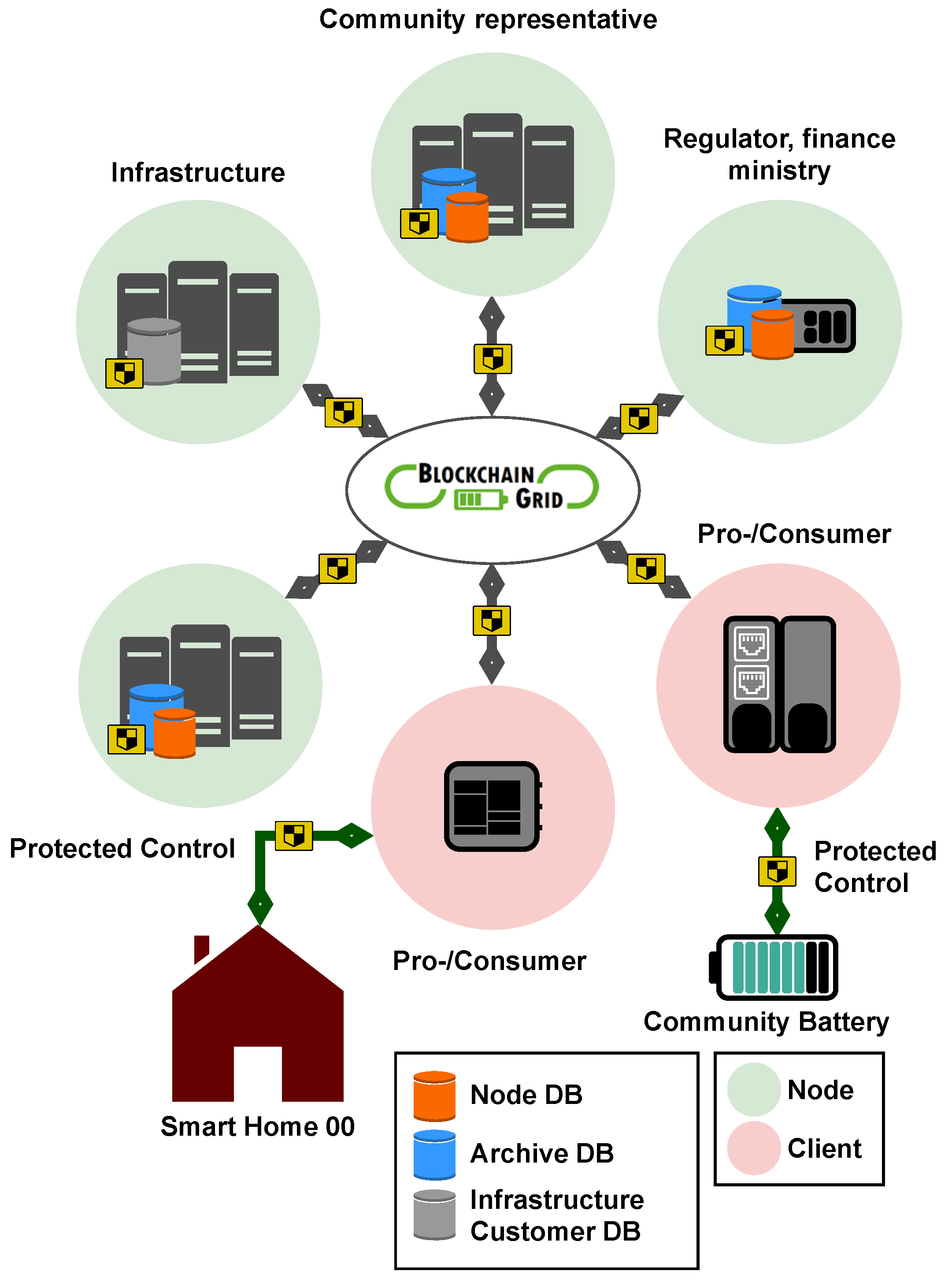
2. Blockchain System Architecture

The Ethereum client Open Ethereum is the basis for the Blockchain architecture adopted in this project. Various servers and communication components are seen in Figure 1. Any node in the network can write data into the Blockchain. In the project, this is constrained and limited by the LEC platform manager at the infrastructure server. Additionally, the grid controller is hosted on this server, which generates optimal set-points for various flexibility controllers in the LEC and facilitates the market processes. The consensus algorithm on how to agree on new blocks is Proof-of-Authority, in which only authorized participants, called sealers, are allowed to generate blocks containing transactions and add them to the Blockchain. Participants can also be dynamically added or removed by the platform operator.

There are two different types of nodes, full nodes, which also perform the sealing to add blocks, and nodes located at measurement devices, sensors and actuators. The latter ones do not perform any sealing and can be configured to run as light clients to lower the hardware requirements. Light clients do not keep the whole chain data, but can participate in the network by trusting other nodes.

Every 15 s a new block is added, which is much lower than the 1 min sample time. This way, it is guaranteed that transactions are processed in time for the next sample. Every sample, PQ values are fed into the Blockchain at all the buses in the grid. Information for the Blockchain, smart contracts, the role of participants and access rights are stored in the infrastructure server. Real customer data (name, address, customer number) is associated with an Ethereum account address. This is managed and used by the Distribution System Operator (DSO) for billing-relevant purposes. The data exchange between the infrastructure server and the participants takes place via an encrypted connection. To be able to access the data, each participant receives an access identifier (username and password). This identifier is linked to the customer data by the infrastructure server.

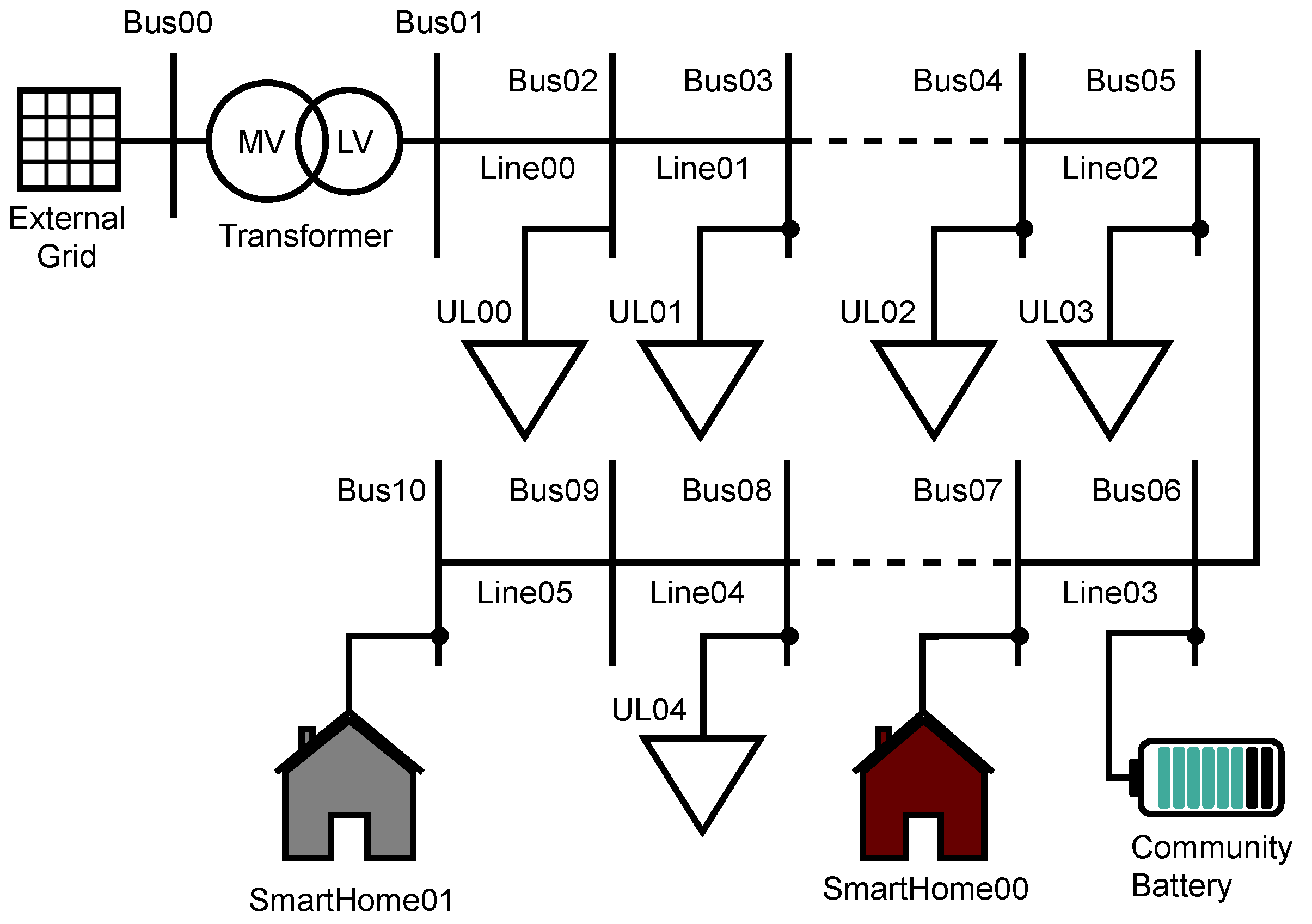
3. Stratified Control Scheme for Low Voltage Distribution Networks

In this section, the authors present a stratified control scheme for voltage management in a three-phase low voltage distribution grid, as part of an LEC. They are inherently unbalanced, as discussed in Section 1, and the unbalance is further increased by DERs and next-gen loads. It is paramount to minimize it for safe system operation. A methodology to generate optimal set-points at a certain number of controllable buses at critical nodes is presented. Flexibilities connected at these buses actively track these set-points using model predictive control. In this research, smart buildings with various flexibilities, such as electric storage and heat-pumps, are connected at these critical nodes (see Section 5).The upper level controller consists of an optimal power flow model using a three-phase unbalanced holomorphic embedding load flow method (HELM-OPF), characterized in Section 4 and mixed-integer quadratic programming model predictive control (MiQ-MPC) is described in Section 5. Figure 2 describes a general model schematic and Figure 3 describes the control structure.

It is to be noted that the grid level controller does not directly provide set-points to the individual flexibilities as it does not have any device model information. It instead generated set-points at the buses where they are connected (at the PCC). This leads to the preservation of sensitive flexibility information and helps protect consumer privacy.

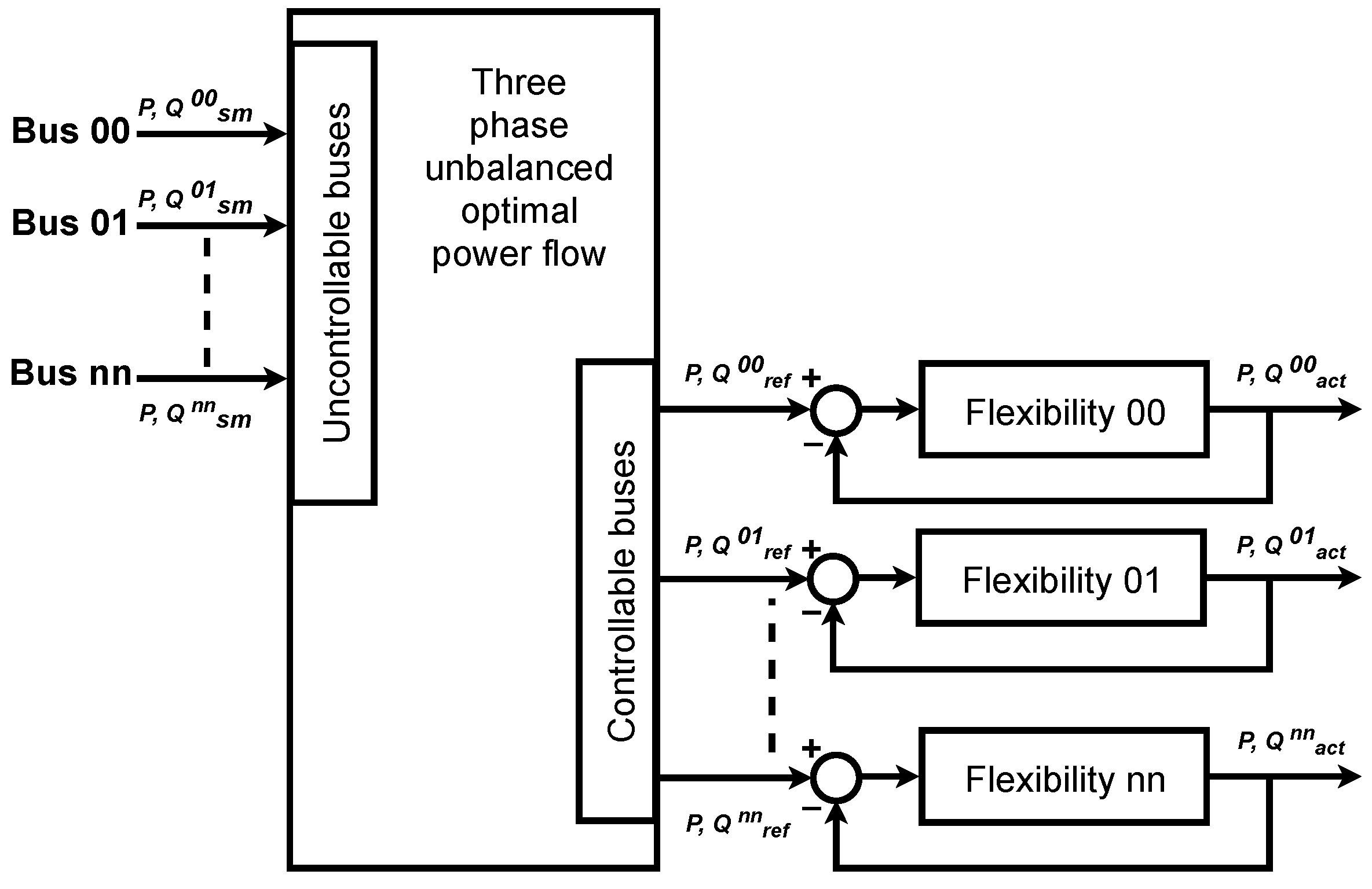
4. Grid Controller Formulation

Power grids are nonlinear and non-convex and it is strenuous to solve the OPF problem associated with it. Various methods have been presented to handle such non-linearity and non-convexity. In this paper, a solution to OPF using the non-convex optimization method is chosen. This is based on the method developed in [9]. It uses a three-phase unbalanced holomorphic embedding load flow method (HELM) with a genetic algorithm to generate optimal set-points, a HELM-OPF method. The reason for using HELM is due to its robustness and ability to converge to a high voltage operable solution irrespective of its initial conditions (very high or low loading conditions) [9]. Using HELM, OPF is given access to the entire search space.

Three-phase unbalanced low voltage distribution network models are adopted from [33].

OPF is formulated as,

$$\begin{array}{ccc}\hfill & \underset{u}{\mathrm{minimize}}J=\hfill & \hfill F(x,u)\\ \hfill & \mathrm{subject}\mathrm{to}\hfill & \hfill H(x,u)& =0,\hfill \\ \hfill & \hfill & \hfill G(x,u)& \le 0,\hfill \end{array}$$

(1)

where, x and u are state and input variable sets. Input variables are the active and reactive power injections at controllable buses; state variables are voltage and phase angles (see Figure 3).

$F(x,u)$ is the objective function for the HELM-OPF problem. Typical objectives are total generator cost and loss minimization in the network.

4.1. Objective Functions

In this paper, three objective functions are used. Objective Section 4.1.1 is used to minimize three-phase unbalance and is used online. Objective Section 4.1.2 is used to choose the best number of controllable buses where flexibilities are needed. Objective Section 4.1.3 is used to determine the voltage controllability.

4.1.1. Three-Phase Unbalance Minimization

The objective function is chosen to minimize three-phase voltage unbalance. There are various methods to realize the objective and, in this paper, balanced voltages are used as a reference, which is illustrated in Equation (2).

$$\begin{array}{cc}\hfill minimizeJ& =\sum _{t\in T}\sum _{k\in {\rm Y}}\sum _{p\in P}{(real\left(V_{k,balanced}^{p,t}\right)-real\left(V_k^{p,t}\right))}^2\hfill \\ \hfill & +{(imag\left(V_{k,balanced}^{p,t}\right)-imag\left(V_k^{p,t}\right))}^2,\hfill \end{array}$$

(2)

where $\mathrm{{\rm Y}}$ represents buses in the network (see Section 4.1.3 for various scenarios), T represents simulation time and $P\in phases(a,b,c)$. The rectangular coordinate system is used to represent voltages and to balance both magnitudes and phase angle; therefore, both real and imaginary parts of complex voltages are used. In Section 7, three different forms of the objective function are defined.

$G(x,u)$ and $H(x,u)$ are the equality and inequality constraints. Three-phase unbalanced HELM developed in [9] is used as equality constraints.

Inequality constraints with respect to distribution grids are as follows,

$$\begin{array}{cc}\hfill P_{Lo{w}_i}^p& \le P_{P{V}_i}^p\le P_{Hig{h}_i}^p\hfill \end{array}$$

(3)

$$\begin{array}{cc}\hfill |V_{Lo{w}_i}^p|& \le |V_i^p|\le |V_{Hig{h}_i}^p|\hfill \end{array}$$

(4)

$$\begin{array}{cc}\hfill t_{Lo{w}_i}& \le t_i\le t_{Hig{h}_i}\hfill \end{array}$$

(5)

$$\begin{array}{cc}\hfill {\theta }_{Lo{w}_i}& \le {\theta }_i\le {\theta }_{Hig{h}_i}\hfill \end{array}$$

(6)

$$\begin{array}{cc}\hfill s_{Lo{w}_i}& \le s_i\le s_{Hig{h}_i}\hfill \end{array}$$

(7)

$$\begin{array}{cc}\hfill Q_{Lo{w}_i}^p& \le Q_{P{V}_i}^p\le Q_{Hig{h}_i}^p\hfill \end{array}$$

(8)

$$\begin{array}{cc}\hfill P_{i,j}^p& \le P_{Hig{h}_{i,j}}^p\hfill \end{array}$$

(9)

$$\begin{array}{cc}\hfill P_{i,j}^{p2}& +Q_{i,j}^{p2}\le S_{Highi,j}^{p2}\hfill \end{array}$$

(10)

$$\begin{array}{cc}\hfill |I_{i,j}^p|& \le |I_{Hig{h}_{i,j}}^p|\hfill \end{array}$$

(11)

$$\begin{array}{cc}\hfill {\mathrm{\Theta }}_{Lo{w}_i}^p& \le {\mathrm{\Theta }}_i^p-{\mathrm{\Theta }}_j^p\le {\mathrm{\Theta }}_{Hig{h}_i}^p.\hfill \end{array}$$

(12)

The variables in the equations above are defined in the

Table 1. Nomenclature.

Variable	Definition
P	Active power
Q	Reactive power
V	Voltage
t	Transformer tap position
$\theta$	Transformer phase shift angle
s	shunt reactances or capacitances
I	Branch current magnitudes
$\mathrm{\Theta }$	Voltage phase angle

.

4.1.2. Optimal Placement of Flexibilities

It is essential to optimally place the flexibilities in the grid to have the maximum impact on voltage control. Various methods are used to determine the location where flexibility is connected.

Most predominantly, they can be broadly classified into two types. Firstly, the voltage sensitivity method, like the quasi-dynamic simulation, is used similarly to those in [4]. This method is limited since it only provides information about the buses where most voltage violations occur for a given period. This method had several limitations since power grids are nonlinear and non-convex.

Secondly, an optimal heuristic technique uses flexibility models and OPF to determine the best location using a non-convex solver. Variations of this method are detailed in [34,35,36]. In this paper, the authors present a method that is based on the heuristic technique but does not need any flexibility models, which need to be included in the HELM-OPF formulation. They are determined based on only active and reactive power injections at the buses. This method applies to any flexibility or DER unit without including any information about it. Mixed-integer programming, along with the HELM method from the previous Section, is used, and the associated objective function is presented in Equation (13). This is a modification of Equation (2), where an additional integer term is added to determine the best location.

$$\begin{array}{cc}\hfill minimizeJ& =\sum _{k\in \Omega }(D{C}_k+E\sum _{p\in P}{(real\left(V_{k,balanced}^p\right)-real\left(V_k^p\right))}^2\hfill \\ \hfill & +{(imag\left(V_{k,balanced}^p\right)-imag\left(V_k^p\right))}^2),\hfill \end{array}$$

(13)

where $C_k$ represents the binary variable associated with each bus in the network leading to a set of optimal controllable buses. D and E are weights associated with the objectives.

4.1.3. Voltage Controllability

During the research, the voltage unbalances minimization at the buses, directly depending on the optimal schedule.

In other words, voltages at all the buses are controlled by PQ powers at flexibilities and at only certain controllable buses (Case 01). Therefore, using Equation (2), the following three scenarios are chosen:

$$\mathsf{{\rm Y}}=\left\{\begin{array}{cc}\Omega \hfill & \mathrm{all}\mathrm{buses}(\mathrm{Case}01)\hfill \\ V\hfill & \mathrm{voltage}\mathrm{violation}\mathrm{buses}(\mathrm{Case}02)\hfill \\ C\hfill & \mathrm{optimal}\mathrm{controllable}\mathrm{buses}(\mathrm{Case}03),\hfill \end{array}\right.$$

(14)

where V represents all the buses where voltage violation was observed. C represents optimal controllable buses from Section 4.1.2. The results of the three scenarios are discussed in Section 7.

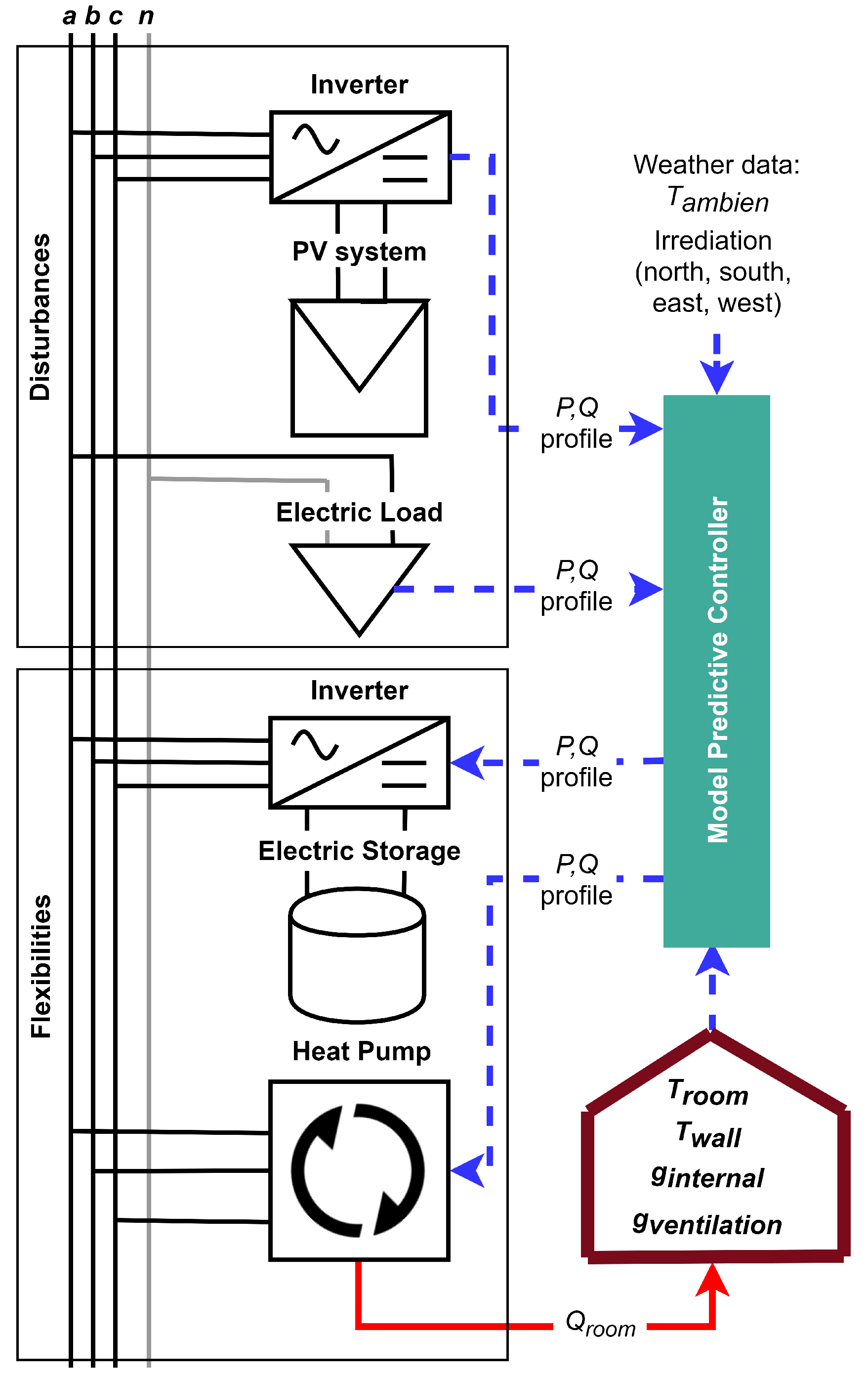
5. Flexibility Controller Formulation

Flexibilities in this paper are mostly hosted in smart building energy management systems with the addition of a large community battery.

5.1. Smart Building Thermal Model

Smart building models are derived from [32]. Various smart building models with varying degrees of complexity are used in this paper. Figure 4 represents a three-phase unbalanced smart building energy management system with various single and three-phase loads.

Thermal models of smart buildings are based on typical buildings in Austria and are derived from [32] and are represented as a discrete state-space system with a sampling time of 15 min.

$$x_{room}(t+1)=A_{room}{x}_{room}\left(t\right)+B_{room}{u}_{room}\left(t\right).$$

(15)

Room and structure temperatures are the state variables in $x_{room}$ (see Equation (16)). $T_{structure}$ is the temperature of the floor, walls and ceiling. $A_{room}$ and $B_{room}$ are the system matrices of the building.

$$x_{room}=\left[\begin{array}{c}{T}_{structure}\\ T_{room}.\end{array}\right]$$

(16)

Equations (17) and (18) are the lower and upper limits of the temperatures in Equation (16).

$$T_{structure}^{min}\le T_{structure}\left(t\right)\le T_{structure}^{max}$$

(17)

$$T_{room}^{min}\le T_{room}\left(t\right)\le T_{room}^{max}.$$

(18)

$u_{room}$ describes the input vector of the state–space system. The only controllable variable is $q_{room}$, which is the heat flowing into the room.

$$u_{room}=\left[\begin{array}{c}{q}_{room}\\ T_{ambienttemperature}\\ i_{north}\\ i_{east}\\ i_{south}\\ i_{west}\\ g_{internalgain}\\ g_{ventilationlosses},\end{array}\right]$$

(19)

where $T_{ambienttemperature}$ is the outdoor temperature, solar irradiation from all directions is $i_{north,east,south,west}$ and $g_{internalgain,ventilationlosses}$ are the internal gains and ventilation losses, respectively.

Equation (20) represents the limits on $q_{room}$. In this paper, only heating is assumed and therefore, $q_{room}$ is greater than zero.

$$0\le q_{room}\left(t\right)\le q_{room}^{max}.$$

(20)

5.2. Constraints on Heat-Pump

Equations (21) and (22) are the single and three-phase powers of the heart pump, respectively. Coefficient of performance ($co{p}_{heatpump}$) is assumed to be time-invariant and constant.

$$P_{heatpump}\left(t\right)=\frac{q_{room}\left(t\right)}{co{p}_{heatpump}}$$

(21)

$$P_{heatpump}^p\left(t\right)=\frac{q_{room}\left(t\right)}{3co{p}_{heatpump}},$$

(22)

where $P_{heatpump}$ is the active power and $co{p}_{heatpump}$ is the coefficient of performance. $p\in phases(a,b,c)$. In order to model the on-off heat-pump model of certain house models, a binary variable $B_{heatpump}$ is used. This can be observed in Equation (23).

$$P_{heatpump}\left(t\right)=B_{heatpump}{P}_{heatpump}^{rated}.$$

(23)

The pump in the heat pump consists of an induction motor and is assumed to be lossless. Additionally, it is assumed to be operating at constant power factor ($p{f}_{heatpump}$) as described in Equation (24), using which, the reactive power ($Q_{heatpump}$) is calculated.

$$\begin{array}{cc}\hfill Q_{heatpump}\left(t\right)& =tan\left(co{s}^{-1}\left(p{f}_{heatpump}\right)\right)\hfill \\ \hfill & P_{heatpump}\left(t\right).\hfill \end{array}$$

(24)

$P_{heatpump}$ and $Q_{heatpump}$ ≥ 0, since the heating period is considered, are described in Equations (25) and (26)

$$0\le P_{heatpump}\left(t\right)\le P_{heatpump}^{max}$$

(25)

Constraints on heat pump reactive power limits,

$$0\le Q_{heatpump}\left(t\right)\le Q_{heatpump}^{max},$$

(26)

where $P_{heatpump}^{max}$ and $Q_{heatpump}^{max}$ are rated active and reactive powers, respectively.

5.3. Constraints on Electric Storage

Distributed energy resources are inherently intermittent and it is essential to use their productions to the fullest extent. Therefore, electric storage is gaining importance in recent years. In this paper, the authors have used linear models for electric storage and inverters. This model is also used to represent the community battery along with the inverter model in Section 5.4. The state of charge (SOC) is described in Equation (27), represents the energy balance in electric storage.

$$\begin{array}{cc}\hfill soc(t+1)C_{battery}& =soc\left(t\right)C_{battery}\hfill \\ \hfill & +\mathsf{\Delta }t{\eta }_{battery}{P}_{battery}\left(t\right).\hfill \end{array}$$

(27)

SOC, battery charging and discharging power limits are as follows,

$$so{c}^{min}\le soc\left(t\right)\le so{c}^{max}$$

(28)

$$P_{battery}^{min}\le P_{battery}\left(t\right)\le P_{battery}^{max}.$$

(29)

5.4. Constraints on Inverter

The electric storage described in Section 5.3 is connected to a three-phase inverter. Due to the non-linearity and non-convexity of the three-phase inverter with both active and reactive control along with binary control variable from Section 5.2. In order to maintain the linearity, only active power control is chosen, described in Equations (30) and (31).

$${\left(P_{battery}\left(t\right)\right)}^2={\left(P_{inverter}\left(t\right)\right)}^2.$$

(30)

Per phase inverter is modeled as follows,

$$P_{inverter}\left(t\right)=\sum _p{P}_{inverter}^p\left(t\right).$$

(31)

5.5. Constraints on Controllable Loads

Controllable loads are defined as simple dump loads, which are both single and three-phased. This is done due to the lack of data related to the presence of controllable loads in the field. In the future, this is to be replaced with realistic controllable load models. The constraints on limits of active and reactive powers are defined in Equations (32) and (33). They work with constant power factor $\left(p{f}_{controllableload}\right)$, described in Equation (34).

$$0\le P_{controllableload}^p\left(t\right)\le P_{controllableload}^{max}$$

(32)

$$0\le Q_{controllableload}^p\left(t\right)\le Q_{controllableload}^{max}$$

(33)

$$\begin{array}{cc}\hfill Q_{controllableload}^p\left(t\right)& =tan\left(co{s}^{-1}\left(p{f}_{controllableload}\right)\right)\hfill \\ \hfill & P_{controllableload}^p\left(t\right).\hfill \end{array}$$

(34)

Real smart meter profiles from the Blockchain are used for uncontrollable loads and PV systems for each sample.

5.6. Constraints at Grid Connection Point

The bus at which a smart building is connected is referred to as a grid connection point. $P_{grid}^p$ and $Q_{grid}^p$ takes both positive and negative values. Constraints on active and reactive powers are constrained in Equations (35) and (36).

$$\begin{array}{cc}\hfill P_{grid}^p\left(t\right)& =P_{inverter}^p\left(t\right)+P_{heatpump}^p\left(t\right)\hfill \\ \hfill & +P_{controllableload}^p\left(t\right)+P_{uncontrollableload}^p\hfill \end{array}$$

(35)

$$\begin{array}{cc}\hfill Q_{grid}^p\left(t\right)& =Q_{heatpump}^p\left(t\right)+Q_{controllableload}^p\left(t\right)\hfill \\ \hfill & +Q_{uncontrollableload}^p.\hfill \end{array}$$

(36)

Forecasting of disturbances is carried out using neural networks [37,38]. This method is not described in the paper since it is not the focus. Weather data, such as temperature, are sourced from weather stations in Austria. Irradiation, ventilation losses and internal gains are collected from local sensors and sourced from the iWPP-Flex project. Forecasting uncertainties lead to an issue with the optimal set-points. However, for the sake of simplicity, these conditions are ignored in this paper.

5.7. Objective Function

The objective function used in the smart building is to provide grid support. The three-phase optimal power flow formulation from Section 4 produces optimal active and reactive power schedules, based on an objective function, for various controllable buses. Each smart building can support the grid by tracking the optimal schedules and by controlling various flexibilities, as described in Equation (37).

$$\begin{array}{cc}\hfill J_{gridsupport}& =\sum _t\sum _p{(P_{gridoptimalschedule}^p\left(t\right)-P_{grid}^p\left(t\right))}^2\hfill \\ \hfill & +{(Q_{gridoptimalschedule}^p\left(t\right)-Q_{grid}^p\left(t\right))}^2+.\hfill \end{array}$$

(37)

Equation (38) represents the objective function of a smart building, $J_{gridsupport}$, the individual flexibility objective function, $\mathcal{G}$ and $\mathcal{F}$ are the respective weight. For the sake of simplicity, $J_{gridsupport}$ is to maximize comfort for all smart buildings (Keeping $T_{room}$ at 22 °C).

$$minimizeJ=\mathcal{G}{J}_{gridsupport}+\mathcal{F}{J}_{flexibilityobjective}.$$

(38)

Variables $P_{heatpump}$, $P_{battery}$ and $P_{controllableload}$ are controllable. Grid support is maximized while maintaining comfort with respect to temperature and load demands are being completely met.

6. Control Strategy

The smart buildings that are described in Section 5.1 are controlled hierarchically [32]. Inputs to the stratified controller are the smart meter active and reactive power forecasts ($P_i^{sm},Q_i^{sm}$). The forecasting method is based on convolutional neural networks, and details about it are not presented in this paper. Three-phase unbalanced optimal power flow from Section 4.1.1 generates optimal active and reactive power set-points to controllable buses. The locations of these buses are chosen based on Section 4.1.2 and Equation (13). Since DERs are intermittent in nature, follow daily, weekly and seasonal cycles, these changes are reflected in the optimal set-points. The flexibility controller must be robust enough to accommodate these changes. The authors have chosen a model predictive control to schedule them optimally. MiQ-MPC receives set-points and is used as reference input signals.

Chronological control functions at grid and house level are presented below.

6.1. Grid Control

Grid control performs HELM-OPF described in Section 4 and broadcasts the optimal set-points to various smart buildings in the network. The chronological control events are presented in Algorithm 1.

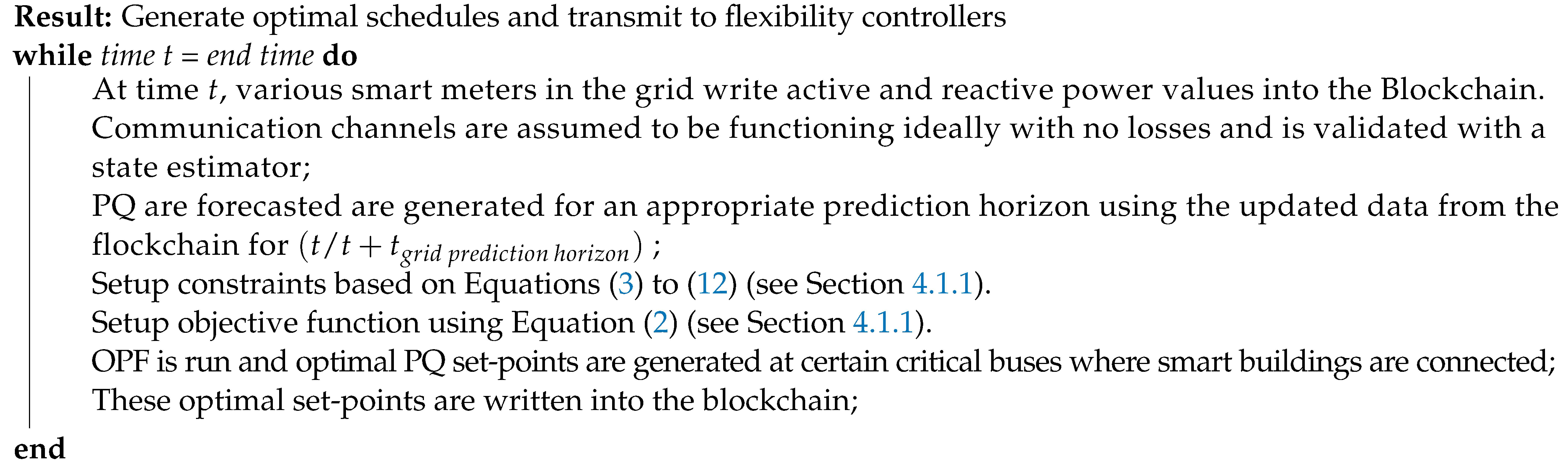
Algorithm 1: Control actions performed at grid level controller

6.2. Flexibility Control

Quadratic programming with mixed-integer is used with continuous and on/off heat-pumps, respectively (see Section 5.2). The chronological control events are presented in Algorithm 2.

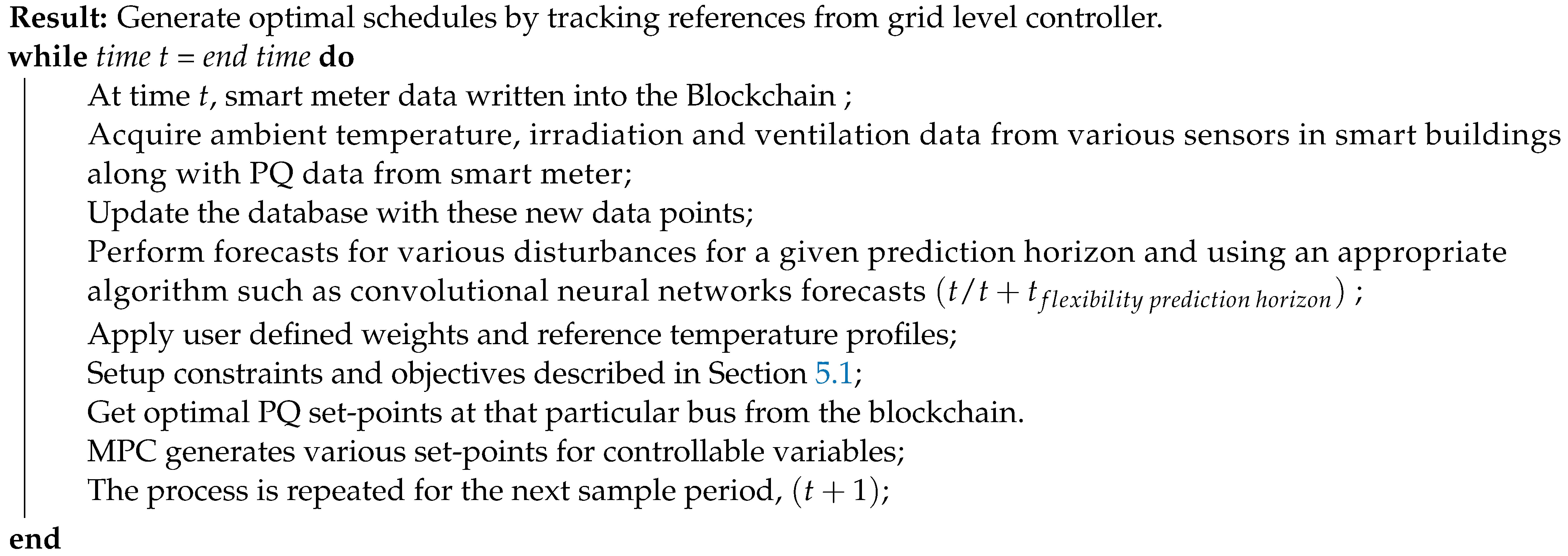
Algorithm 2: Control actions performed at flexibility level controller

7. Simulation and Results

The grid selected for the analysis is a 264 bus three-unbalanced low voltage distribution network (three-phase four-wire) in Austria, represented in Figure 5. It contains single and three-phased loads along with DER units. The network is simplified by summing all the loads and generations at each bus to obtain one load per bus. Loads are active and reactive power profiles from real smart meters in the grid. For the sake of privacy, the data are not visualized or presented in this paper.

A simulation is performed to determine the optimal buses at which flexibilities are to be placed as mentioned in Section 4.1.2 and by using the objective function in Equation (13). The optimal buses are presented in

Table 2. Simulation parameter limits for optimal buses.

Optimal Buses	Bus 020	Bus 031	Bus 038	Bus 042	Bus 045	Bus 055	Bus 058	Bus 067	Bus 069	Bus 077
$P_{heat-pump}^{max}$ (kW)	5	9	8	9	5	9	5	6	9	-
$P_{heat-pumpphase}$ (kW)	1P	1P	3P	1P	3P	1P	1P	1P	1P	-
$P_{battery}^{max}$ (kW)	20	20	27	24	26	27	21	20	22	30
$C_{battery}$ (kWh)	42	31	32	29	36	49	39	34	41	120
$P_{controllableload}^{max}$ (kW)	19	16	10	6	15	10	9	16	13	-
$P_{controllableloadphase}$ (kW)	1P	3P	3P	1P	3P	1P	3P	3P	1P	-
Optimal Buses	Bus 081	Bus 091	Bus 092	Bus 094	Bus 099	Bus 112	Bus 117	Bus 118	Bus 140	Bus 148
$P_{heat-pump}^{max}$ (kW)	6	6	5	5	8	8	7	8	7	8
$P_{heat-pumpphase}$ (kW)	3P	1P	1P	1P	1P	1P	3P	1P	3P	1P
$P_{battery}^{max}$ (kW)	24	22	27	26	26	23	20	27	26	21
$C_{battery}$ (kWh)	28	32	26	29	41	30	43	44	31	31
$P_{controllableload}^{max}$ (kW)	13	8	9	9	16	5	11	5	15	9
$P_{controllableloadphase}$ (kW)	3P	3P	3P	1P	3P	3P	1P	1P	1P	1P
Optimal Buses	Bus 168	Bus 169	Bus 171	Bus 184	Bus 207	Bus 217	Bus 225	Bus 234	Bus 238	Bus 241
$P_{heat-pump}^{max}$ (kW)	8	9	5	7	5	5	7	8	8	6
$P_{heat-pumpphase}$ (kW)	3P	3P	3P	1P	3P	3P	1P	3P	1P	1P
$P_{battery}^{max}$ (kW)	22	28	23	27	21	29	27	23	20	24
$C_{battery}$ (kWh)	35	31	26	26	33	38	42	40	27	28
$P_{controllableload}^{max}$ (kW)	16	16	6	11	14	13	12	7	5	11
$P_{controllableloadphase}$ (kW)	1P	1P	3P	3P	1P	3P	1P	3P	1P	3P

and are represented in Figure 5. At these buses, simple single-phase uncontrollable loads are replaced with three-phase flexibilities, smart building or a community battery. Having determined the optimal buses where flexibilities are to be placed, the simulation is performed based on the three cases mentioned in Section 4.1.2. These simulations are benchmarked against real smart meter active and reactive power profiles at the controllable buses where flexibilities are to be placed, and their forecasts and optimal schedules are to be produced by the grid level controller. The simulation is performed for two days between 2019-04-01 00:00:00 and 2019-04-02 23:45:00 with 29 smart buildings and one large community storage (Bus 077). Smart buildings are comprised of single and three-phased flexibilities as described in Section 5 and in Figure 4. Table 2 presents various limits on certain controllable variables for optimal buses.

Figure 6 presents the voltage magnitude results for three scenarios and benchmarks. It can be observed that under and over-voltages (0.95 pu. < voltage < 1.05 pu.) are observed for real and forecasted profiles. The optimal profiles from the grid-level controller have resulted in no voltage violation. The same can be observed for case 01 and 03, as flexibilities are tracking the optimal profiles. The reason for Case 02 to observe over-voltage is because voltage controllability is limited to only controllable buses, as described in Section 4.1.3. In case 01, since all the buses are included, the optimizer is able to mitigate violations. In case 03, since the voltage controllability is the optimal controllable buses, under voltage violation was observed. This is due to the fact that not all the buses are included in the voltage controllability. This enforces that the voltage is a local effect due to power flows in multiple directions. To mitigate voltage violations in all buses, voltage controllability should extend to all buses.

The performance of the flexibilities directly depends on how well they can track the optimal grid schedules. In Figure 7 $P_{grid}$, $P_{gridoptimal}$ and their absolute difference is presented for a smart building connected at Bus 020. Similarly, $Q_{grid}$, $Q_{gridoptimal}$ and their absolute difference is presented in Figure 8. It can be observed that the smart building can track the optimal grid schedule. This depends on the flexibility composition available in the smart building. Therefore, due to this reason, the global optimum cannot be guaranteed. However, from Figure 9, it can be observed that the results are close to the global optimum.

Figure 9 presents the function values for all the scenarios based on the objective in Equation (2). As discussed earlier, it can be observed that the unbalance is minimized for each case when compared to the benchmarks. There is an 85.92%, 64.27%, and 77.02% reduction in three-phase unbalance for Cases 01, 02, and 03, respectively (the imbalances are in Voltage (p.u.) values). Stratified controllers are written in Python, including three-phase unbalanced optimal power flow and model predictive control.

8. Conclusions and Outlook

In this paper, the authors present a stratified control scheme in a peer-to-peer local energy community (see Section 3). It uses a three-phase unbalanced optimal power flow based on holomorphic embedding load flow method and receding horizon control as described in Section 4. Blockchain acts as an enabler by making the data available at all the buses in the grid. Three-phase optimal active and reactive power set-points are generated for controllable buses, which are found using the objective function in Equation (13) in Section 4.1.2. Mixed integer quadratic model predictive control is hosted in flexibility controllers with various electrical connection configurations and thermal models (see Section 5).

An objective function to minimize three-phase voltage unbalance with three use cases is presented in Section 6. Voltage magnitudes for the simulation duration for all the scenarios are presented. It is observed that cases 01 and 03 have completely mitigated the voltage violations. Is observed that there is an 85.92%, 64.27%, and 77.02% reduction of phase unbalance for the three cases. In the context of local energy communities, such a system can provide services to the distribution system operator. Additionally, the objectives defined by the community operator can be included in the grid level control. One other advantage is the ability of individual flexibilities to have their own objectives and simultaneously support the grid. One of the limitations is the intense communication needs as all the measurement devices and the controllers are to be connected to the blockchain to send and receive data.

In future work, the stratified control structure needs to be integrated with the peer-to-peer energy market and modified accordingly to perform the market settlement process. Additionally, a control scheme should be tested with various other real networks for stability and replication analysis. The smart building models used in this paper are linear. More realistic, nonlinear models are to be used to obtain a better optimal profile tracking along with appropriate sizing of various flexibilities. Additionally, reactive power control is limited in flexibility models. By implementing them, better tracking of set-points is possible, leading to a solution being closer to a global optimum.

References

1. Babaiahgari, B.; Ullah, M.H.; Park, J.D. Coordinated Control and Dynamic Optimization in DC Microgrid Systems. Int. J. Electr. Power Energy Syst. 2019, 113, 832–841. [Google Scholar] [CrossRef]
2. Bazmohammadi, N.; Tahsiri, A.; Anvari-Moghaddam, A.; Guerrero, J.M. A Hierarchical Energy Management Strategy for Interconnected Microgrids Considering Uncertainty. Int. J. Electr. Power Energy Syst. 2019, 109, 597–608. [Google Scholar] [CrossRef]
3. Dou, C.X.; Liu, B. Hierarchical Hybrid Control for Improving Comprehensive Performance in Smart Power System. Int. J. Electr. Power Energy Syst. 2012, 43, 595–606. [Google Scholar] [CrossRef]
4. Brandstetter, M.; Schirrer, A.; Miletić, M.; Henein, S.; Kozek, M.; Kupzog, F. Hierarchical Predictive Load Control in Smart Grids. IEEE Trans. Smart Grid 2017, 8, 190–199. [Google Scholar] [CrossRef]
5. Glavitsch, H.; Bacher, R. Optimal Power Flow Algorithms. In Control and Dynamic Systems; Elsevier: Amsterdam, The Netherlands, 1991; Volume 41, pp. 135–205. [Google Scholar] [CrossRef]
6. Dommel, H.W.; Tinney, W.F. Optimal Power Flow Solutions. IEEE Trans. Power Appar. Syst. 1968, PAS-87, 1866–1876. [Google Scholar] [CrossRef]
7. Stott, B.; Hobson, E. Power System Security Control Calculations Using Linear Programming, Part I. IEEE Trans. Power Appar. Syst. 1978, PAS-97, 1713–1720. [Google Scholar] [CrossRef]
8. Stott, B.; Hobson, E. Power System Security Control Calculations Using Linear Programming, Part II. IEEE Trans. Power Appar. Syst. 1978, PAS-97, 1721–1731. [Google Scholar] [CrossRef]
9. Rao, B.V.; Kupzog, F.; Kozek, M. Three-Phase Unbalanced Optimal Power Flow Using Holomorphic Embedding Load Flow Method. Sustainability 2019, 11, 1774. [Google Scholar] [CrossRef] [Green Version]
10. Sun, Y.; Li, P.; Li, S.; Zhang, L.; Sun, Y.; Li, P.; Li, S.; Zhang, L. Contribution Determination for Multiple Unbalanced Sources at the Point of Common Coupling. Energies 2017, 10, 171. [Google Scholar] [CrossRef] [Green Version]
11. Yong, J.Y.; Ramachandaramurthy, V.K.; Tan, K.M.; Mithulananthan, N. A Review on the State-of-the-Art Technologies of Electric Vehicle, Its Impacts and Prospects. Renew. Sustain. Energy Rev. 2015, 49, 365–385. [Google Scholar] [CrossRef]
12. Karimi, M.; Mokhlis, H.; Naidu, K.; Uddin, S.; Bakar, A. Photovoltaic Penetration Issues and Impacts in Distribution Network—A Review. Renew. Sustain. Energy Rev. 2016, 53, 594–605. [Google Scholar] [CrossRef]
13. Al-badi, A.H.; Ieee, S.M.; Elmoudi, A.; Metwally, I.; Ieee, S.M.; Al-wahaibi, A.; Al-ajmi, H.; Bulushi, M.A. Losses Reduction in Distribution Transformers. In Proceedings of the International Multi Conference of Engineers and Computer Scientists 2011 (IMECS 2011), Hong Kong, China, 16–18 March 2011; Volume II. [Google Scholar]
14. Gnacinski, P. Windings Temperature and Loss of Life of an Induction Machine Under Voltage Unbalance Combined With Over- or Undervoltages. IEEE Trans. Energy Convers. 2008, 23, 363–371. [Google Scholar] [CrossRef]
15. Lee, S.Y.; Wu, C.J. On-Line Reactive Power Compensation Schemes for Unbalanced Three Phase Four Wire Distribution Feeders. IEEE Trans. Power Deliv. 1993, 8, 1958–1965. [Google Scholar] [CrossRef]
16. Soltani, S.; Rashidinejad, M.; Abdollahi, A. Dynamic Phase Balancing in the Smart Distribution Networks. Int. J. Electr. Power Energy Syst. 2017, 93, 374–383. [Google Scholar] [CrossRef]
17. Zeng, X.; Zhai, H.; Wang, M.; Yang, M.; Wang, M. A System Optimization Method for Mitigating Three-Phase Imbalance in Distribution Network. Int. J. Electr. Power Energy Syst. 2019, 113, 618–633. [Google Scholar] [CrossRef]
18. Kaveh, M.R.; Hooshmand, R.A.; Madani, S.M. Simultaneous Optimization of Re-Phasing, Reconfiguration and DG Placement in Distribution Networks Using BF-SD Algorithm. Appl. Soft Comput. 2018, 62, 1044–1055. [Google Scholar] [CrossRef]
19. Soltani, S.; Rashidinejad, M.; Abdollahi, A. Stochastic Multiobjective Distribution Systems Phase Balancing Considering Distributed Energy Resources. IEEE Syst. J. 2018, 12, 2866–2877. [Google Scholar] [CrossRef]
20. Mostafa, H.A.; El-Shatshat, R.; Salama, M.M.A. Multi-Objective Optimization for the Operation of an Electric Distribution System With a Large Number of Single Phase Solar Generators. IEEE Trans. Smart Grid 2013, 4, 1038–1047. [Google Scholar] [CrossRef]
21. Schweickardt, G.; Alvarez, J.M.G.; Casanova, C. Metaheuristics Approaches to Solve Combinatorial Optimization Problems in Distribution Power Systems. An Application to Phase Balancing in Low Voltage Three-Phase Networks. Int. J. Electr. Power Energy Syst. 2016, 76, 1–10. [Google Scholar] [CrossRef]
22. Wang, K.; Skiena, S.; Robertazzi, T.G. Phase Balancing Algorithms. Electr. Power Syst. Res. 2013, 96, 218–224. [Google Scholar] [CrossRef]
23. Sun, S.; Liang, B.; Dong, M.; Taylor, J.A. Phase Balancing Using Energy Storage in Power Grids Under Uncertainty. IEEE Trans. Power Syst. 2016, 31, 3891–3903. [Google Scholar] [CrossRef] [Green Version]
24. Watson, J.D.; Watson, N.R.; Lestas, I. Optimized Dispatch of Energy Storage Systems in Unbalanced Distribution Networks. IEEE Trans. Sustain. Energy 2018, 9, 639–650. [Google Scholar] [CrossRef]
25. Mateo, V.; Gole, A.M.; Ho, C.N.M. Design and Implementation of Laboratory Scale Static Var Compensator to Demonstrate Dynamic Load Balancing and Power Factor Correction. In Proceedings of the 2017 IEEE Electrical Power and Energy Conference (EPEC), Saskatoon, SK, Canada, 22–25 October 2017; pp. 1–6. [Google Scholar] [CrossRef]
26. Nejabatkhah, F.; Li, Y.W. Flexible Unbalanced Compensation of Three-Phase Distribution System Using Single-Phase Distributed Generation Inverters. IEEE Trans. Smart Grid 2019, 10, 1845–1857. [Google Scholar] [CrossRef]
27. Jia, L.; Yu, Z.; Murphy-Hoye, M.C.; Pratt, A.; Piccioli, E.G.; Tong, L. Multi-Scale Stochastic Optimization for Home Energy Management. In Proceedings of the 2011 4th IEEE International Workshop on Computational Advances in Multi-Sensor Adaptive Processing (CAMSAP), San Juan, Puerto Rico, 12–15 December 2011; pp. 113–116. [Google Scholar] [CrossRef] [Green Version]
28. Giorgio, A.D.; Pimpinella, L.; Liberati, F. A Model Predictive Control Approach to the Load Shifting Problem in a Household Equipped with an Energy Storage Unit. In Proceedings of the 2012 20th Mediterranean Conference on Control Automation (MED), Barcelona, Spain, 3–6 July 2012; pp. 1491–1498. [Google Scholar] [CrossRef]
29. Chen, C.; Wang, J.; Heo, Y.; Kishore, S. MPC-Based Appliance Scheduling for Residential Building Energy Management Controller. IEEE Trans. Smart Grid 2013, 4, 1401–1410. [Google Scholar] [CrossRef]
30. Hidalgo Rodríguez, D.I.; Myrzik, J.M. Economic Model Predictive Control for Optimal Operation of Home Microgrid with Photovoltaic-Combined Heat and Power Storage Systems. IFAC-PapersOnLine 2017, 50, 10027–10032. [Google Scholar] [CrossRef]
31. Godina, R.; Rodrigues, E.; Pouresmaeil, E.; Matias, J.; Catalão, J. Model Predictive Control Home Energy Management and Optimization Strategy with Demand Response. Appl. Sci. 2018, 8, 408. [Google Scholar] [CrossRef] [Green Version]
32. Rao, B.; Kupzog, F.; Kozek, M. Phase Balancing Home Energy Management System Using Model Predictive Control. Energies 2018, 11, 3323. [Google Scholar] [CrossRef] [Green Version]
33. Bazrafshan, M.; Gatsis, N. Comprehensive Modeling of Three-Phase Distribution Systems via the Bus Admittance Matrix. IEEE Trans. Power Syst. 2018, 33, 2015–2029. [Google Scholar] [CrossRef] [Green Version]
34. Prakash, K.; Islam, F.R.; Mamun, K.A.; Ali, S. Optimal Generators Placement Techniques in Distribution Networks: A Review. In Proceedings of the 2017 Australasian Universities Power Engineering Conference (AUPEC), Melbourne, VIC, Australia, 19–22 November 2017; pp. 1–6. [Google Scholar] [CrossRef]
35. Tang, Y.; Low, S.H. Optimal Placement of Energy Storage in Distribution Networks. IEEE Trans. Smart Grid 2017, 8, 3094–3103. [Google Scholar] [CrossRef]
36. Suresh, M.C.V.; Belwin, E.J. Optimal DG Placement for Benefit Maximization in Distribution Networks by Using Dragonfly Algorithm. Renew. Wind Water Sol. 2018, 5, 4. [Google Scholar] [CrossRef]
37. Kobylinski, P.; Wierzbowski, M.; Piotrowski, K. High-Resolution Net Load Forecasting for Micro-Neighbourhoods with High Penetration of Renewable Energy Sources. Int. J. Electr. Power Energy Syst. 2020, 117, 105635. [Google Scholar] [CrossRef]
38. Chaturvedi, D.; Sinha, A.; Malik, O. Short Term Load Forecast Using Fuzzy Logic and Wavelet Transform Integrated Generalized Neural Network. Int. J. Electr. Power Energy Syst. 2015, 67, 230–237. [Google Scholar] [CrossRef]
Figure 1. Blockchain System Architecture implemented in the BlockchainGrid project at the LEC in Austria.
Energies 14 03290 g001
Figure 2. General schematic of a three-phase unbalanced distribution grid with a medium-voltage/low-voltage transformer, uncontrollable loads (UL), smart buildings and a community battery system.
Energies 14 03290 g002
Figure 3. Structure of the stratified control scheme. Inputs to the grid controller are forecasted profiles of smart meter active and reactive ( P i s m , Q i s m ) profiles from loads located at various uncontrollable buses (Bus 00, Bus 01, …, Bus nn). Outputs are optimal P i r e f and Q i r e f set-points that are calculated using HELM-OPF and fed into individual flexibility controllers. Using these reference profiles, the flexibility controller produces optimal set-points for its flexibility portfolio, which are P i a c t and Q i a c t using MiQ-MPC. Based on the available flexibility type and their sizing, the buildings may not be able to perfectly tract the reference profiles generated by the grid controller.
Energies 14 03290 g003
Figure 4. Schematic of three-phase HEMS with various electrical and thermal components. It can be observed that the electric appliances can have single, two or three-phase connection configurations.
Energies 14 03290 g004
Figure 5. Topology of a real network in Austria with various smart buildings and a community battery.
Energies 14 03290 g005
Figure 6. Voltage magnitude distributions for benchmarks, optimal and three cases with under and over voltages for each of the cases.
Energies 14 03290 g006
Figure 7. Per phase active powers at point of common coupling, grid optimal schedule and absolute difference between them at Bus 020.
Energies 14 03290 g007
Figure 8. Per phase reactive powers at the point of common coupling, optimal grid schedule and the absolute difference between them at Bus 020. Due to the lack of reactive power control in flexibility models and devices working at a fixed power factor, reference profiles are not being followed when compared to active power tracking in Figure 7. This is done for the sake of simplicity, to maintain the linearity of flexibility models and their controllers.
Energies 14 03290 g008
Figure 9. Objective function values for the three scenarios (see Section 4.1.3). Objective function values from Equation (2) are reduced to voltage (p.u.) for better understanding of results.
Energies 14 03290 g009