
Development of Online Adaptive Traction Control for Electric Robotic Tractors
by
Idris Idris Sunusi
1,2, 
Jun Zhou
1,*, 
Chenyang Sun
1,
Zhenzhen Wang
1,
Jianlei Zhao
1 and
Yongshuan Wu
1 1
College of Engineering, Nanjing Agricultural University, Nanjing 210031, China
2
National Agricultural Extension and Research Liaison Services, Ahmadu Bello University, Zaria 1067, Nigeria
*
Author to whom correspondence should be addressed.
Energies 2021, 14(12), 3394; https://0-doi-org.brum.beds.ac.uk/10.3390/en14123394
Submission received: 12 March 2021
/
Revised: 1 June 2021
/
Accepted: 1 June 2021
/
Published: 9 June 2021
(This article belongs to the Special Issue Control Design for Electric Vehicles)
Abstract
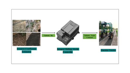
:Estimation and control of wheel slip is a critical consideration in preventing loss of traction, minimizing power consumptions, and reducing soil disturbance. An approach to wheel slip estimation and control, which is robust to sensor noises and modeling imperfection, has been investigated in this study. The proposed method uses a simplified form of wheels longitudinal dynamic and the measurement of wheel and vehicle speeds to estimate and control the optimum slip. The longitudinal wheel forces were estimated using a robust sliding mode observer. A straightforward and simple interpolation method, which involves the use of Burckhardt tire model, instantaneous values of wheel slip, and the estimate of longitudinal force, was used to determine the optimum slip ratio that guarantees maximum friction coefficient between the wheel and the road surface. An integral sliding mode control strategy was also developed to force the wheel slip to track the desired optimum value. The algorithm was tested in Matlab/Simulink environment and later implemented on an autonomous electric vehicle test platform developed by the Nanjing agricultural university. Results from simulation and field tests on surfaces with different friction coefficients (μ) have proved that the algorithm can detect an abrupt change in terrain friction coefficient; it can also estimate and track the optimum slip. More so, the result has shown that the algorithm is robust to bounded variations on the weight on the wheels and rolling resistance. During simulation and field test, the system reduced the slip from non-optimal values of about 0.8 to optimal values of less than 0.2. The algorithm achieved a reduction in slip ratio by reducing the torque delivery to the wheel, which invariably leads to a reduction in wheel velocity.
1. Introduction
In precision agriculture, the primary objectives are to improve production efficiency; reduce environmental degradation; and, more importantly, optimize the use of available resources such as energy, water, seeds, and fertilizer. In line with these objectives, electric tractors (ET) were introduced into agricultural productions. In ET, electric motors are used for traction, while chemical batteries, fuel cells, or ultracapacitors are used as energy sources. Compared to internal combustion engines, electric tractors have the advantages of having fewer components, being emission-free, having high efficiency, being independent from petroleum, and having quiet and smooth operations [1]. ET is also easy to handle because its dynamic can be easily realized by controlling the electric motor. ET’s advantages are realized because electric motors, which are its prime components, have a quick torque response and can be easily controlled by manipulating voltage [2]. To leverage on the advantages of electric vehicle technologies, electric tractors were developed for pesticide applications and other agricultural purposes. The main advantages are that such operation does not require high power; as such, their power demand can be met by the electric batteries [3,4,5,6,7,8]. Though much progress has been achieved on improving batteries’ performance, its energy density is still lower than that of conventional fuel, and the cost is still high [9,10,11,12,13]. Studies have been conducted with the sole aim of increasing the operating range of electric vehicles, and these studies have led to the development of various techniques for reducing power consumption. Online traction control and optimization is among the most promising researched areas.
A critical role is played by traction control in vehicles’ dynamic control. It improves drive efficiency, increases safety, and makes the system more stable [14]. Traction is the force that propels the vehicles in the direction of motion; it is generated by the friction between the wheels and the road/terrain surface. Friction is dependent on many variables, including road type, road conditions, wheel types, wheel slip, vertical load, tire wear state, and temperature [14,15]. Additionally, it is affected by operation parameters such as velocity and acceleration. Researchers in vehicles’ dynamic controls have lumped all these factors affecting the friction into a single parameter call friction coefficient. This parameter is found to be dependent on the wheel slip. There exists an optimum value of slip, for each road type and set of conditions, at which the friction coefficient is high. Since the slip affects friction coefficient and invariably the traction force, it is used as the control variable in most of the traction control. Therefore, traction controls are designed to regulate slip to the optimum value. By so doing, degradation of driving performances resulting during sudden acceleration in poor road conditions is eradicated. One more benefit is that the power consumption is also reduced. Unfortunately, traction control is generally difficult because of the uncertainty and nonlinearity associated with the friction between the wheel and road surface [16].
The earliest studies on traction control were based on maximum transmissible torque estimation (MTTE), model following control (MFC), and velocity feedback. However, the most recent studies were based on slip feedback. This change in focus is connected to the fact that there is a strong relationship between slip rate and traction force, and the ease of slip estimation due to the development and availability of improved sensors [17,18,19,20,21,22].
Previous studies were mainly directed to address the problems of estimating the velocity of the vehicle. Difficulties, such as drift caused by DC offset while using accelerometers, high cost of optical sensors, and their susceptibility to contamination by mud or water necessitated the development of traction control that does not depend on vehicle velocity estimation [23,24,25,26,27]. Model following control (MFC) does not need information on vehicle velocity or acceleration; it is based on only wheel torque and wheel velocity. However, to accommodate worst-case scenario in a real field environment, high control gain is required in tuning the controllers, and this constrains the performance of the method [2,28,29,30]. MTTE is another means of traction control without the need to estimate vehicle speed. It is an improved form of MFC, and it centers on comparing the maximum torque developed based on the vehicle dynamic model and the one measured using sensors. When wheels slip, a difference is obtained between the two torques, and this difference is feedback to the controller. The method’s major drawbacks are high sensitivity to variation in wheel inertia and steering difficulty in situations where the wheels have different friction coefficients [29,31,32].
Traction control that is more robust to changes in terrain types, the unknown wheel-terrain conditions, and does not have the limitations of MFC and MTTE was achieved through slip feedback control. However, it is only applicable where a reliable estimate of vehicle velocity is available. Because it was found experimentally that the traction is highest at the slip range 15–30% for many terrains, earlier studies on slip feedback pegged the optimum slip within this range [33]. However, it was found that the optimum value of slip is dependent on tires, operation parameters, and road conditions. These have led to the development of slip controls based on a real-time estimate of the optimum slip, which correspond to high friction between tire and road surfaces. Lookup tables were used to estimate optimum slip, and gave a satisfactory performance on the various roads. Because lookup-table-based systems are detuned to consider the worst scenario, such as wet or icy roads, a suboptimal controller is usually obtained [16].
The most recent research trend is the online estimation of optimum slip for different terrains in various conditions. In [33], the performances of fuzzy logic and sliding mode observer were tested for optimum slip estimation. The study established that observer techniques are appropriate for online estimation of peak adhesion coefficients for different tire-road surface conditions. In [34], the optimal slip value was obtained by taking the first derivative of the slip–adhesion function, the point at which the derivative is equal to zero is taken as the point of optimum slip. The main problem of the method is that it gives an average value of the optimum slip. Furthermore, studies have shown that it mainly estimates high slip changes such as the change from dry road to gravel [35]. Additionally, machine learning applications such as the support vector machine (SVM) and artificial neural network (ANN) have been applied in estimating optimum slip, especially in a situation of low changes in slip value (same road and condition). However, the problem of a tradeoff between generality and estimation speed remains [36].
Due to its ability to perform good unbiased estimation, the recursive least square algorithm (RLS) has been employed to estimate road friction conditions [37]. The algorithm also has a fast response speed, strong anti-jamming capability, and can deal with nonlinearities associated with complex tire models [38,39].
This work’s main objective is to develop an algorithm for the online traction control of electric vehicles used in agricultural fields. The original contribution lies in combining the robustness of sliding mode controller and observer, with the simplicity of the Burckhardt model, to accurately estimate the optimum maximum friction coefficient and the slip ratio at which it occurs. The use of sliding mode observers to estimate the longitudinal wheel force has eliminated the use of expensive sensors in measuring the force. In essence, the study includes developing an optimum slip estimation algorithm by using the Burckhardt traction model, and the design of integral sliding mode controller for tracking the optimum slip. The systems’ performance was evaluated in the Matlab/Simulink environment. Finally, the system was implemented on an electric vehicle test platform and tested in different terrain types.
2. Materials and Methods
2.1. Vehicle Modelling
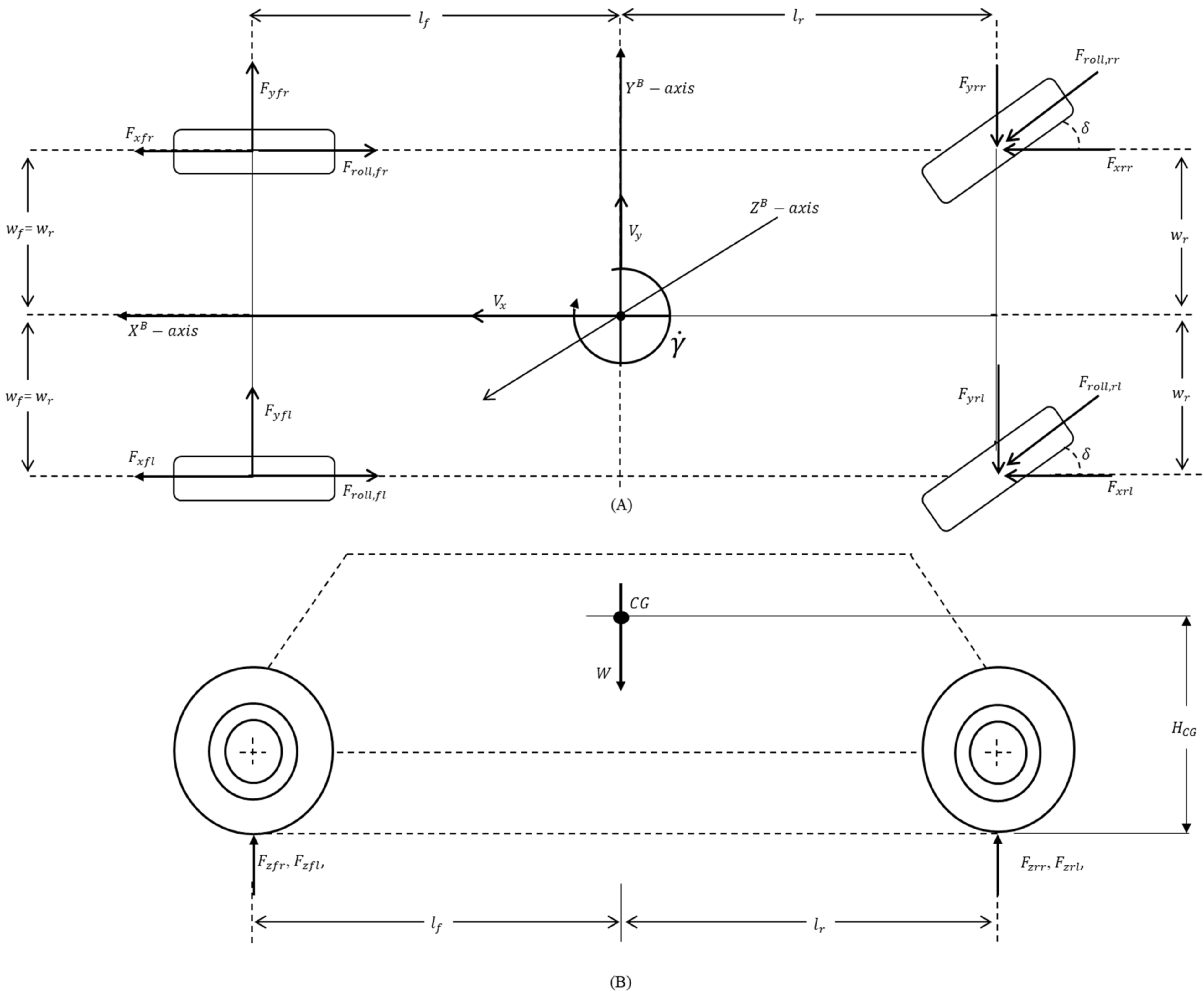
Four degrees of freedom vehicle model was established by considering the motion along the x, y, and z-axis, also considered is the yaw moment along the z-axis. As depicted in Figure 1, the vehicle has a rear-wheel steering system. The x and y axes reside in the ground plane, while the z-axis is perpendicular to the plane of x-y.
Because low speed of operations and flat terrain are considered, the effect of aerodynamic force and grade resistance were neglected to simplify the model. The machine is designed to work in unstructured terrain where soil under the wheels may not be the same. The following are the equations necessary for development and analysis of traction control.
Longitudinal force on the vehicle:
Lateral force on the vehicle:
Yaw moment of the vehicle:
where denotes the mass of the vehicle at center of gravity (CG); denotes the longitudinal acceleration of the vehicle; denotes the lateral acceleration of the vehicle; denotes the longitudinal velocity of the vehicle; denotes the lateral velocity of the vehicle; denotes the yaw rate of the vehicle; and denotes the steering angle.
stands for the longitudinal tire-road friction force for the wheels; stands for the lateral tire-road friction force for the wheels; stands for the rolling resistance force on wheels direction of travel; the subscript, , in , , and stands for and , respectively, with as front left; front right; rear left, and , rear right, respectively.
stands for distance from the vehicle center of gravity to axis that passed through the center of the front wheels; , distance from the vehicle center of gravity to the axis that passed through the center of the rear wheels; and front and rear wheelbase (equal length); , height of the center of gravity; and , the center of gravity.
Vertical forces acting on each wheel are defined as follows [40,41]:
where , , , and are the vertical force on the front right, front left, rear left, and rear right wheel, respectively; , is acceleration due to gravity; and .
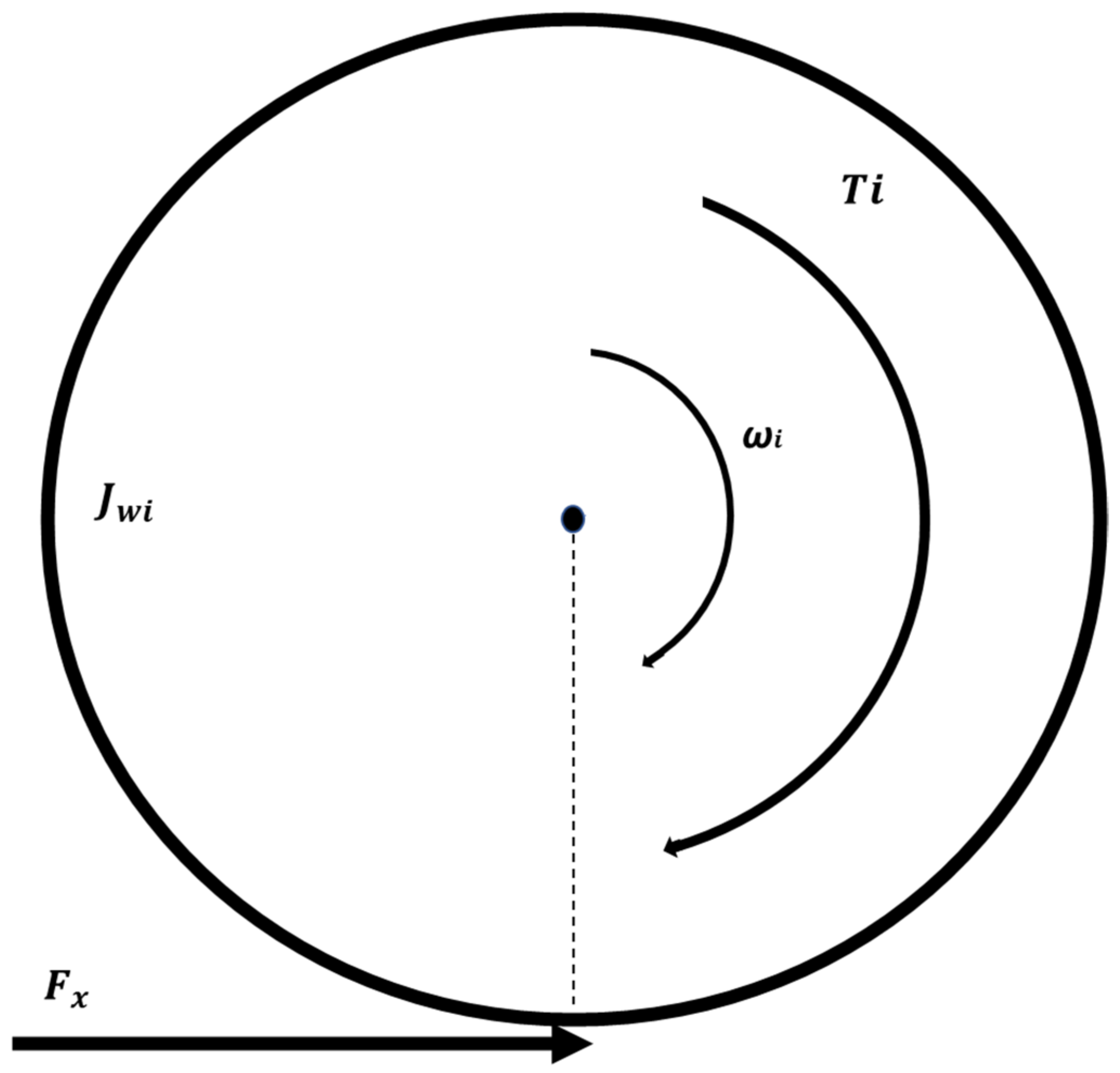
The dynamic of each wheel model can be described by the torque balance of the system in Figure 2, as shown in Equation (5):
where stands for the wheel inertia including motor and reducer; the torque transmitted to the wheels; , wheels rotational acceleration; and , wheel radius.
Wheels longitudinal slip is defined in Equation (6). To avoid a situation whereby the denominator of the slip function becomes zero, which will lead to an infinite value for the slip, a small constant value of 0.05 m/s was set as the minimum value for the slip function denominator.
where stands for wheel longitudinal slip and stands for wheel rotational speed.
The road friction coefficient , which is a nonlinear function of many physical variables including the velocity of the vehicle, the road surface conditions, and slip ratio, is defined as
2.2. Slip Dynamic Based on a Simplified Vehicle Model
The slip dynamic, which is the basis for formulating traction control algorithm, is developed in this section. In order to reduce computational demand on controller, the following simplifications were made in the slip dynamics: it is assumed that viscous torque developed at the wheels’ axles is negligible compared to the torque developed by the longitudinal force, and the yaw rate and lateral acceleration were also set to zero. Due to weight transfer, the tractive force that develops at each of the wheels is assumed to be different. Furthermore, it is assumed that the wheels longitudinal velocity (), and the vehicle longitudinal velocity are greater than or equal to zero ( and ). To control traction or speed of the vehicle, the torque delivered to the wheels by the electric motor is the parameter to be manipulated; therefore, the torque is the control input. Because the structures of the traction models of each of the wheels is similar, method for controlling the tractive force of only one wheel is going to be described. These simplifications may cause some uncertainties; however, real systems are far from being idealistic, uncertainties and unmodelled dynamics are inevitable, and robust controllers are usually used to take charge of these systems’ limitations [42].
The simplified longitudinal acceleration model based on one-wheel dynamics, derived from Equation (1), is given.
From Equation (6), the wheels rotational speed as a function of slip ratio and vehicle speed can be written as
When the slip function in Equation (6) is differentiated, the following function is obtained:
While the state variables in Equation (10) are , the wheel rotational acceleration and , the vehicle longitudinal acceleration, the variable of interest in the design of the slip controller is the slip ratio. Therefore, the slip dynamic model in (10) was manipulated to make the slip ratio and vehicle velocities the state variables.
By substituting Equations (5) and (9) into Equation (10), the following model for slip dynamic function is obtained:
For the sake of simplicity purpose, we take
And
Therefore, the slip dynamic in Equation (11) can be written as
2.3. Wheel Longitudinal Force Observer
In this section, an observer is proposed to identify the longitudinal force of each wheel. Due to the high cost of commercially available sensors for online measurement of tire longitudinal force, efficient technique of estimation for these forces is strongly recommended. The fast dynamics of wheels’ vertical forces make the longitudinal force, which is dependent on the wheel’s vertical force, unsuitable for adaptive compensation. Additionally, the large uncertainty in the friction coefficient between the terrain and the wheel makes it unsuitable for robust compensation because of the need for high loop gain [43]. Therefore, an observer was designed to estimate the longitudinal force. Due to finite convergence; insensitivity to modeling errors; modeling uncertainties; and measurement noise, a sliding mode observer was chosen [44,45,46,47,48,49,50]. Values of vehicle mass and wheel inertia, accurate measurement of wheel torque, and speed were used in the observer models.
Design of the Observer
Because of the lack of cost-effective sensors for measuring longitudinal force, observers are used to estimate the force from the measurement of other variables. The use of the observer also solves the problem of noise in the measuring sensors. An observer was designed to estimate the friction force between the tire and the soil using wheel angular velocity, torque, and wheel dynamic model. In the observer’s design and implementation, numerical differentiation to obtain angular acceleration was avoided because of its sensitivity to measurement noise and quantization, as reported in [43]. Under the assumption that wheel inertia () is known, first-order sliding mode observer was designed as follows.
First, based on the procedure described in [3,43,51], the wheel torque balance in Equation (5) is estimated as
where is the state estimate of the ‘wheel’s angular acceleration; is the state estimate of the ‘wheel’s angular velocity; and is a discontinuous input signal for the observer.
The discontinuous input signal for the observer in Equation (15) is defined as
where is the observer gain, and is the the sliding variable, which is the difference between the measured and estimated wheel rotational speed.
The discontinuous signum function in Equation (16) is defined as
By differentiating Equation (17), and substituting Equations (5), (15) and (16), the expression in Equation (19) is obtained
As the dynamic function in Equation (19) approaches zero, the discontinuous input signal will approach , thereby getting an estimate of . The function can only take the values of and zero, so it determines the sign of
The condition for the sliding variable to converge to zero in finite time was obtained by formulating the Lyapunov function, , [52]. The function is defined as the positive definite function of the estimation error, :
The sliding condition that guarantees the attractivity of is obtained by differentiating Equation (20) as
By substituting the error dynamic in Equation (19) into Equation (21), the following expression is obtained:
This implies that
Because is and the is always if is chosen such that the following inequality is satisfied
It will give
Satisfying the conditions in Equation (20) and the inequality in (24) proves that the sliding variable is asymptotically stable.
Theoretically, the input signal of the sliding mode observer switches at an infinitely high frequency. However, in reality, it is impossible to have such an ideal input signal, so the system oscillates at a limited frequency, with both high- and low-frequency components [53]. Therefore, an equivalent value of the frictional force () was obtained from the low-frequency component of by using lowpass filter. So, only the convergence of the low-frequency component of discontinuous signal was required to estimate the longitudinal force [43,51,54].
2.4. Wheel Terrain Interaction and Optimum Slip Estimation
It has been found that the value of the frictional force between the wheel and the terrain varied with wheel slip, and a particular slip at which the frictional force is high exists for all the terrains. As a result of this, a lot of traction prediction models that relate to wheel slip, wheel longitudinal force, and other wheel-terrain parameters have been developed. Some of the developed models are purely theoretical, while others are empirical or semi-empirical. The semi-empirical models are computationally faster than the theoretical ones. They are more general in terms of applicability in comparison to purely empirical ones [8]. Because the tractor is designed to work on concrete, road, firm soil, and agricultural farms, a model with broad applicability as well as simplicity is required. Due to its relatively simple structure, high accuracy in fitting traction data, and broad applicability in many driving conditions, the Burckhardt tire model was used to characterize this work’s traction force [55,56]. Compared to the magic formula and other models, which are more accurate, the Burckhardt tire model provided a good tradeoff between modeling accuracy and computational cost [50].
The model equation as a function of lambda () is described as
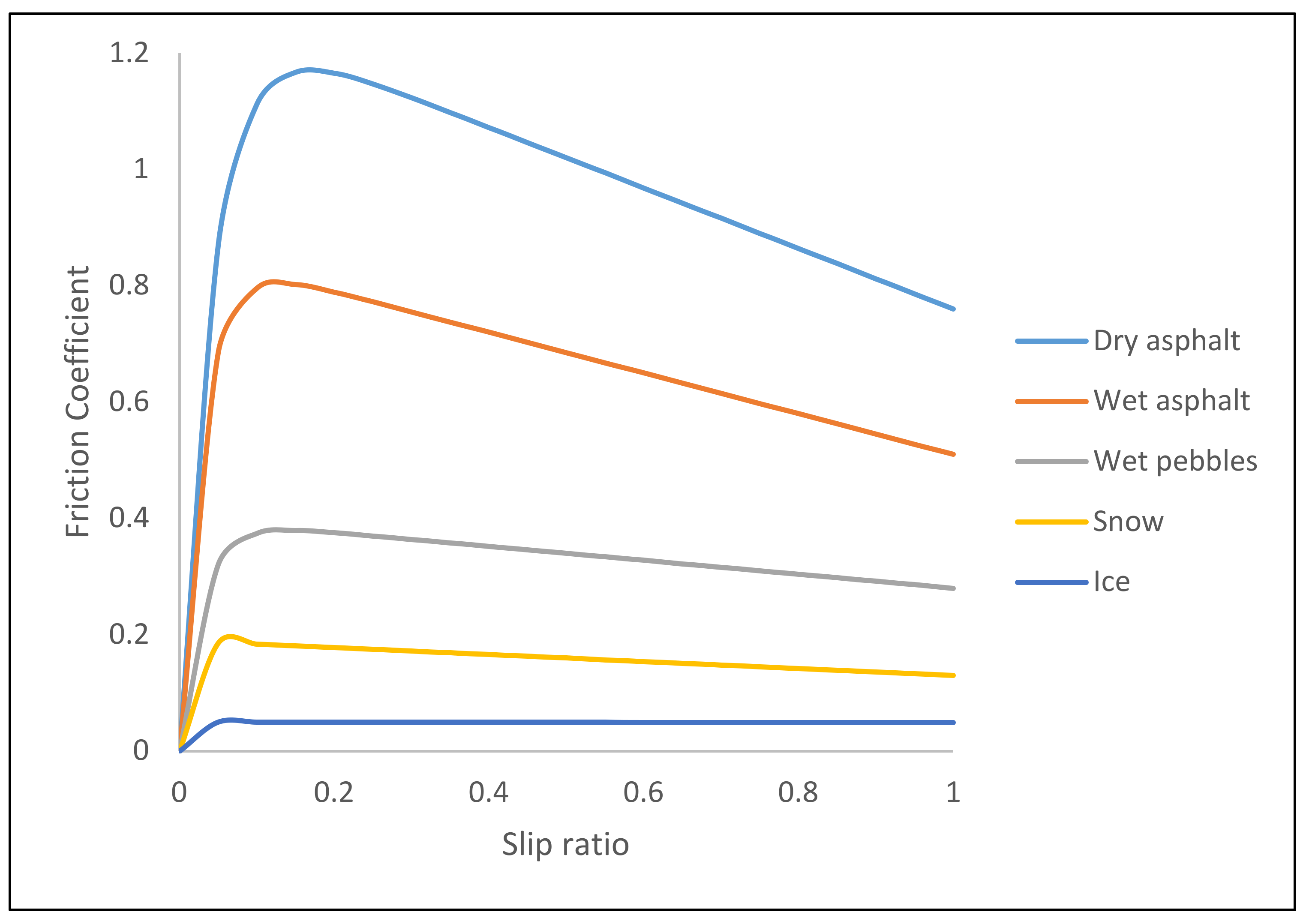
where the parameters are constant variables that are different for different terrain. The values for the parameters for some terrains, including high and low friction coefficient surfaces such as dry concrete and snow, are presented in Table 1.
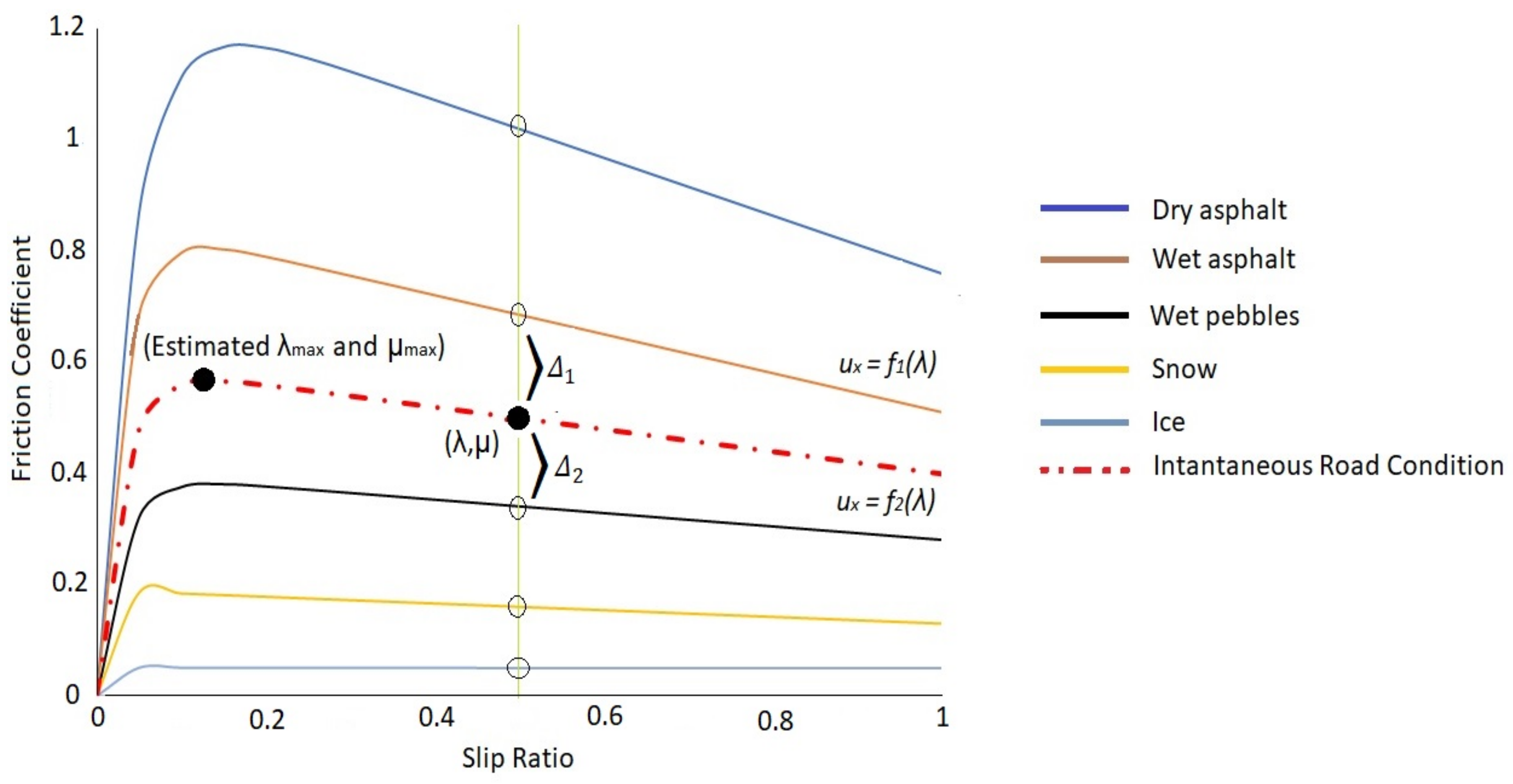
The main problem is that the values of the model parameters are not available for all the diverse groups of terrains in the real world, and the available ones are not fixed; even for a particular terrain, they change with the change in surface condition. Moreover, as shown in Figure 3, the friction coefficient changes with the change in the slip ratio, and it reaches a peak point at a particular value of slip (optimum), beyond which the value starts to decline.
For high traction, the longitudinal force needs to be controlled at that optimum value of slip. A simple and feasible interpolation method was put forward for estimating the instantaneous values of the parameters, maximum friction coefficient, and the optimum slip for different terrains in previous studies [58,59]. The principle of operation of the method is shown in Figure 4, and the process is as follows.
- Step 1.
- By estimating the frictional force as in Section 2.3 and substituting the value equation (7), the instantaneous value of friction coefficient is obtained, while the instantaneous value of slip was obtained from Equation (6).
- Step 2.
- Using the instantaneous value of slip () and the model parameters of the five different terrain types shown in Table 1, five sets of transient values for friction coefficient () are calculated by using Equation (26).
- Step 3.
- Then, five sets of error values () are generated, by subtracting the estimate friction coefficient from the calculated ones ().
- Step 4.
- The two smallest error values ( and ) from step 3 are selected.
- Step 5.
- Using Equation (26) and the values of soil parameters () at the two points where and are obtained, two functions are generated:
- Step 6.
- Using and from step 4 and the functions and from step 5, a new function is reconstructed to estimate the maximum friction coefficient and the corresponding slip values at which it occurs (Figure 4 and Equation (29)).
- Step 7.
- By differentiating Equation (29) and setting the value to zero, the optimum slip (), at which the friction coefficient is maximum is obtained. The maximum friction coefficient can be obtained as in Equation (30)where is the maximum tire-road friction coefficient and is the corresponding slip ratio of .
3. Traction Control Design
The procedure of developing a controller for achieving the system’s objective of forcing the system to follow the desired optimum slip is described in this section.
3.1. Controller Design and Analysis
Due to the need of having high robustness to bounded parameter variations and the modeling imperfections that exist in wheel-terrain interaction systems, and also the issue of unmodeled dynamics due to pitch and roll moments, a sliding mode control (SMC) technique was proposed in this study. SMC has shown superior performance to other controllers such as PI in our previous study [3]. The controller was first designed without considering parameter variations, and later it was made robust to bounded parametric variations. As in all SMC design processes, the sliding surface was designed first, then a control law, that forced and retained the system at the sliding surface was designed.
3.1.1. The Sliding Surfaces Design
Designing a sliding surface for a second and higher-order systems results in exponential convergence of the state errors to zero, while in the first-order systems it resulted in a vertical line, which does not yield exponential convergence, in the phase plane. Furthermore, the dynamics outside the sliding surface become difficult to control [43]. In such cases, integral sliding mode control is used to ensure the state error’s exponential convergence, even when the system dynamic is not equal to zero. One more advantage of integral sliding mode control is that it eliminates the reaching phase completely. An auxiliary sliding surface was designed as follows [51,60]:
where represents the auxiliary sliding surface; the optimum slip ratio; a positive constant that determines the convergence rate, a dummy variable used for integration, and a constant value that shifts the sliding surface in the phase plane to ensure that the auxiliary sliding mode starts from the beginning without any reaching phase, for all initial conditions (that is, ).
Equation (31) becomes
The dynamic of the system in (34) was solved by change of variables, such that
So, if , then and ; hence, by substituting these values, Equation (34) becomes
As given in [60], the solution the inhomogeneous ordinary differential equation (ODE) gives in Equation (36) is then the dynamic of , and it is given as
By expressing Equation (37) in the original variable and simplifying, the following value was obtained:
Equation (38) has shown that for any nonzero initial slip error (), the integrated error converges to a nonzero value. However, the variable of interest is the slip error, not the integrated error; therefore, Equation (38) was differentiated once to the slip error as follows:
So, it can be seen from (39) that the error approaches zero as time () approaches infinity, with an exponential rate of .
3.1.2. Control Law Design
By assuming that the dynamic model’s initial conditions are known, asymptotic output tracking can be achieved by developing a sliding mode control law that compensates for the bounded disturbance in the slip dynamic and drives the sliding variable to zero as time increases.
By taking the derivative of the auxiliary sliding surface in Equation (33), we get
Substituting Equation (32) into (40), and assuming that the derivative of the reference slip is zero (), the following expression was obtained:
The slip dynamic from Equation (14) is substituted into (41), and it becomes:
So, the problem of stabilizing the slip dynamics is now reduced to that of forcing auxiliary sliding variable in Equation (42) to zero, and this was achieved by designing a stabilizing control input .
In order to design a stabilizing control input , a Lyapunov function () was formulated, and the control input (), was chosen such that () is negative definite. The following positive definite function () was chosen as the candidate Lyapunov function:
The time derivative of is given as
Substituting (42) into (44) gives
In order to make (45) negative definite, the control input Tmi should be chosen as
With the parameter as positive integer, and substituting (46) in (45), the following is obtained:
Because Equation (47) is negative definite, it is proved that (43) is a Lyapunov function, and is an asymptotically stable equilibrium. Therefore, the system trajectory will converge to as time approaches infinity, and the sign function in Equation (46) is defined as
3.2. Robust Controller Design
Due to the uncertainty associated with the functions their exact value is not known, only their estimate and is known. As reported in [52], the estimation errors on and were assumed to be bounded by the following:
where is a known function bounding ; , minimum value of the function ; and , the maximum values of the function .
Because the control input () multiplies the function , so the estimates of were chosen as the geometric mean of it bound:
The bound on the estimation error of in Equation (53) was also expressed in another form below:
The parameter will be used later in calculating the controller gain () and it is given as:
Vertical load on the wheels, wheels radius, and rolling resistance were assumed to be of unknown exact value; this was due to the weight transfer that is caused by longitudinal acceleration, roll and pitch acceleration, changes in the wheels rolling radius, and the effect of rolling resistance. Therefore, the functions and were modified to consider the bounded disturbances on these vehicle parameters as follows [43,52]:
The bounded interval that is used in calculating controller gain () is also described in terms of vehicle system parameters follows [43,52]:
where is the minimum weight on a wheel; the estimated weight; the maximum deviation of weight on a wheel; the minimum wheel rolling radius; the maximum wheel rolling radius; the estimated value of rolling resistance coefficient; and the maximum deviation of rolling resistance coefficient.
The modified control law, which is robust to bounded disturbance, is estimated as follows:
With this modified control law in (58), the Lyapunov function will be satisfied when the condition in the inequality in (59), which is used to determine the controller gain (), is met.
3.3. Chattering Elimination
The discontinuous sign function was replaced with a hyperbolic tangent function , so that the chattering of the system around which leads to the demand for high control effort, was eliminated [51,52]. The function is defined as follows:
where the steepness of the hyperbolic tangent function is determined by ε value.
The control was then modified to
4. Matlab Simulations
To verify the validity of the control strategy and to tune the controller gains for satisfactory performance before the actual implementation on a real vehicle, a MATLAB/SIMULINK based model of the electric vehicle was built. The values of fixed and bounded parameters required to simulate the algorithm are shown in Table 2 and Table 3.
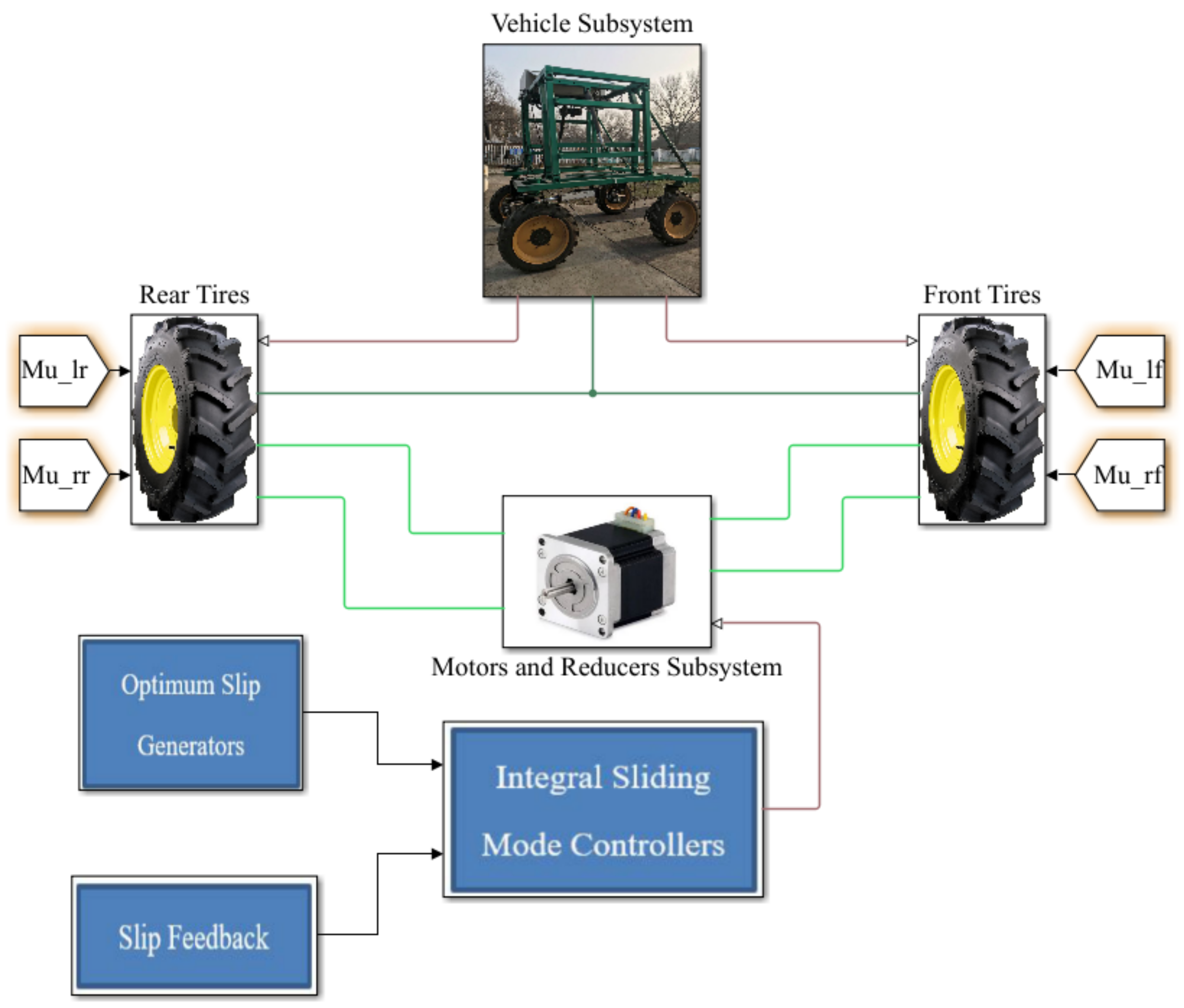
The developed wheel slip controller, which is based on integral sliding mode control, the friction force observer, and the optimum slip estimation algorithms, was also implemented in the environment. The diagram in Figure 5 shows the complete Simulink model.
To evaluate the control functionality and to find an optimal controller setup, several test scenarios that include surfaces with different friction conditions, different speeds, and different longitudinal accelerations were considered during the simulation. The controller gains were tuned to get satisfactory tracking performance.
4.1. Tracking of Friction Coefficient and Robustness Performance
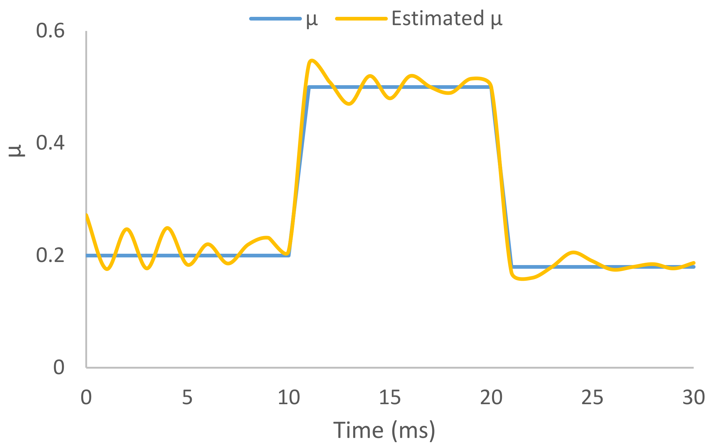
Figure 6 shows the optimum friction coefficient estimation algorithm’s performance on terrains with friction coefficient values of 0.2, 0.5, and 0.18, respectively. The algorithm could track an abrupt change in friction coefficient from 0.2 to 0.5 and 0.5 to 0.18, respectively. It converges to a narrow domain, which contains the optimum value within 10 milliseconds (ms).
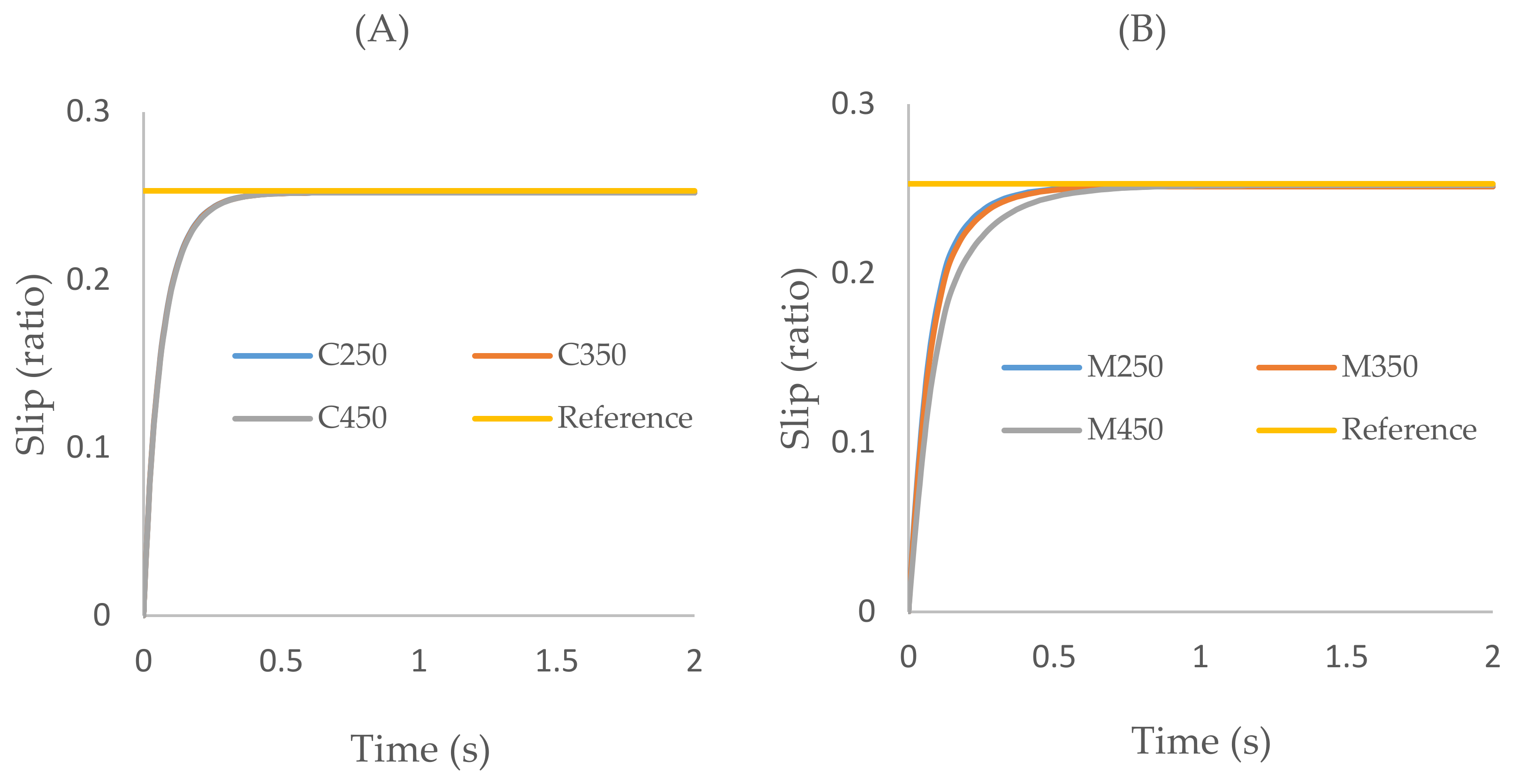
Figure 7 shows the robustness of the control algorithms to the bounded disturbances in the vertical load on the wheels and the changes in rolling resistance of the terrains, respectively. In Figure 7A, the rolling resistance coefficients used for the simulation were 0.1 (C250), 0.15 (C350), and 0.20 (C450), respectively. The corresponding effect on the tracking ability of the control algorithms was negligible as the graph for overlap each other. Figure 7B, the response of control algorithm due change in the weight on the wheel is shown. Three weights of 250 kg (M250), 350 kg (M350), and 450 kg (M450) were used during the simulation. As in the case of rolling resistance, only a little change is observed in the controller response speed. However, the graphs do not overlap. This is an indication that the system is robust to bounded disturbance.
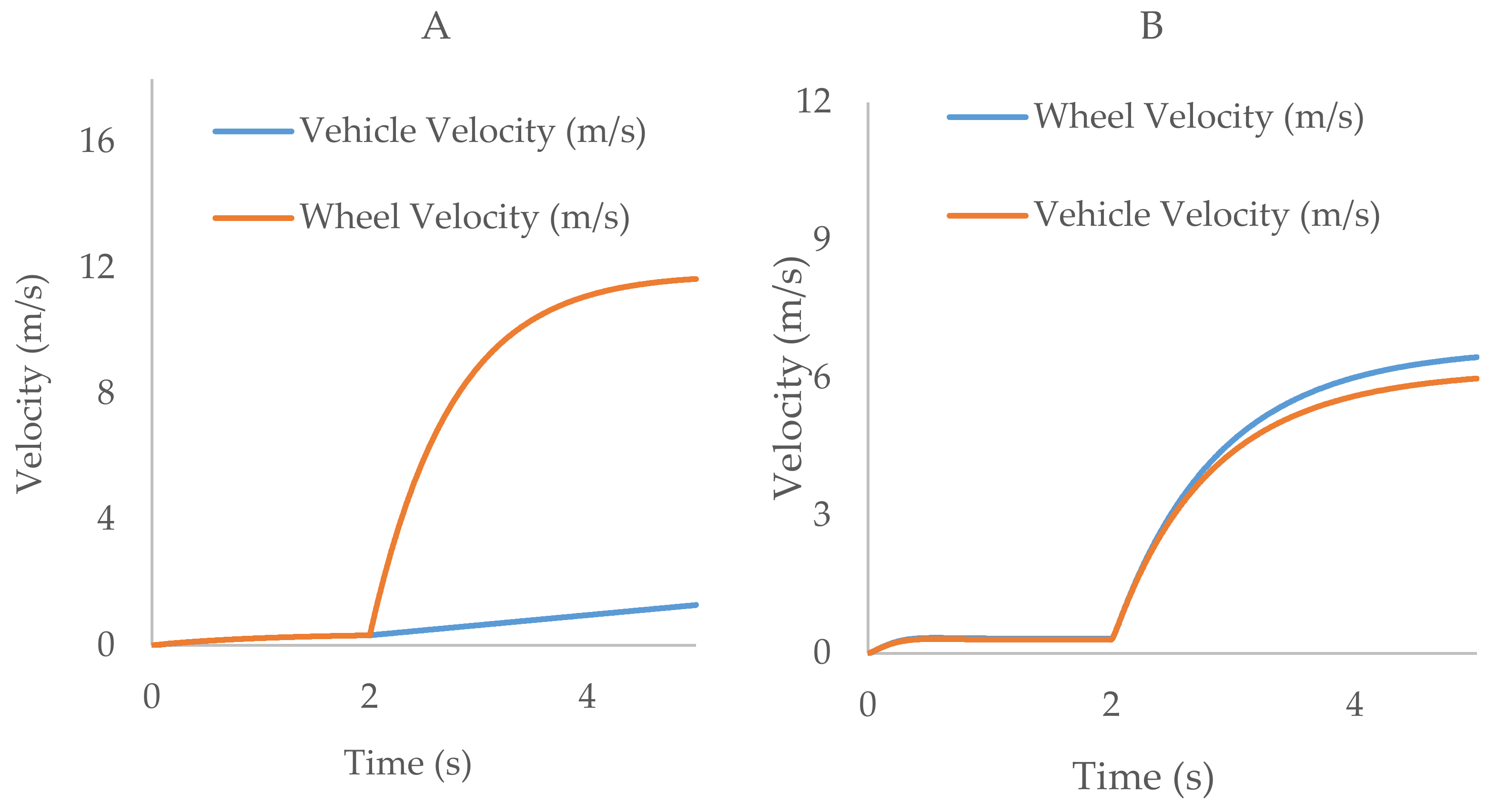
The developed system was simulated for acceleration performances, with and without the traction control algorithm, respectively, in a low μ surface (0.2). In each case, a step input was applied at the accelerator pedal at 2 s; as a result, the wheel speed increased rapidly and diverged from that of the vehicle when the controller was not used (Figure 8A). At 5 s, the wheel speed reached over 11 m/s, while the vehicle speed was just 1.3 m/s. In the second instance of the simulation, in which the controller was used to the system, the wheel and vehicle velocity were regulated to about 6.4 and 6.0 m/s in 5 s, respectively (Figure 8B).
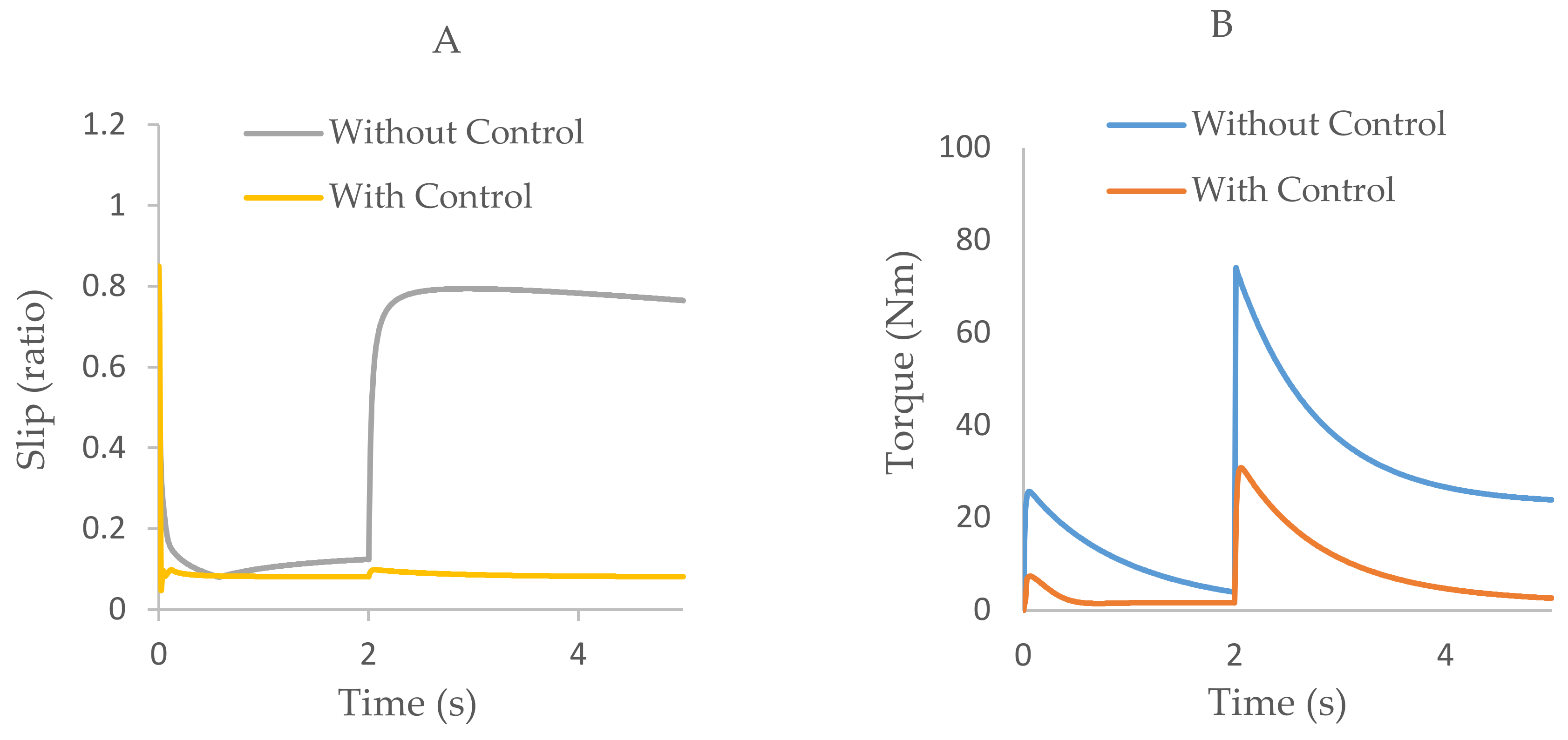
Furthermore, accelerating the vehicle without the controller leads to an increase in the slip from the values around 0.1 before 2 s to a value up to 0.80 after 2-s of the simulation. However, when the controller was used, the slip was regulated within the range of the optimum value of 0.08–0.11 (Figure 9A). As shown in Figure 9B, the torque supplied by the motor was regulated to less than 40 Nm, unlike in the first instance when it reached as high as 100 Nm despite not accelerating the vehicle to a value comparable to the increase in wheel velocity. This shows that the increased torque was wasted in slipping the wheels.
4.2. μ Transition Simulation
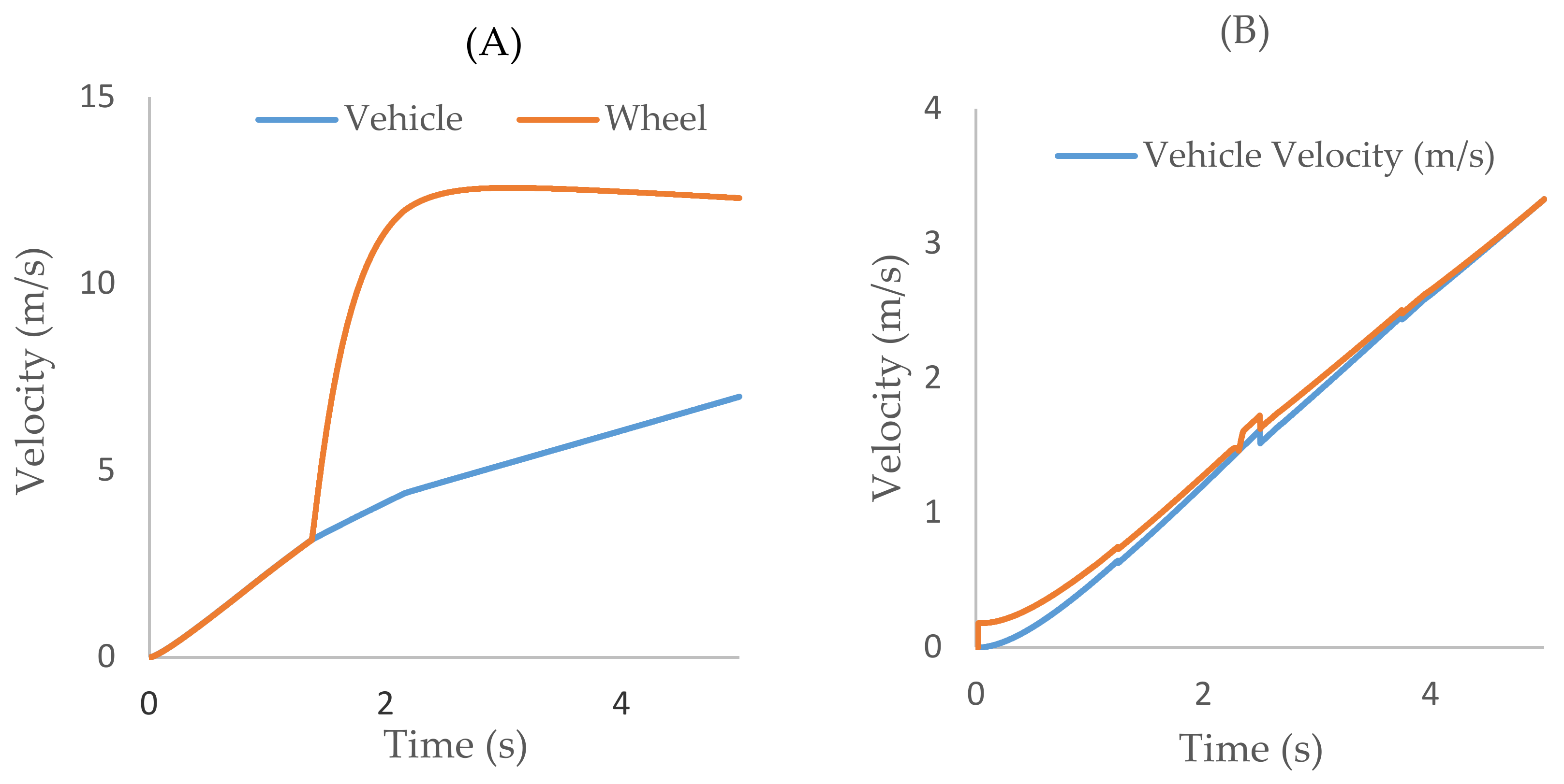
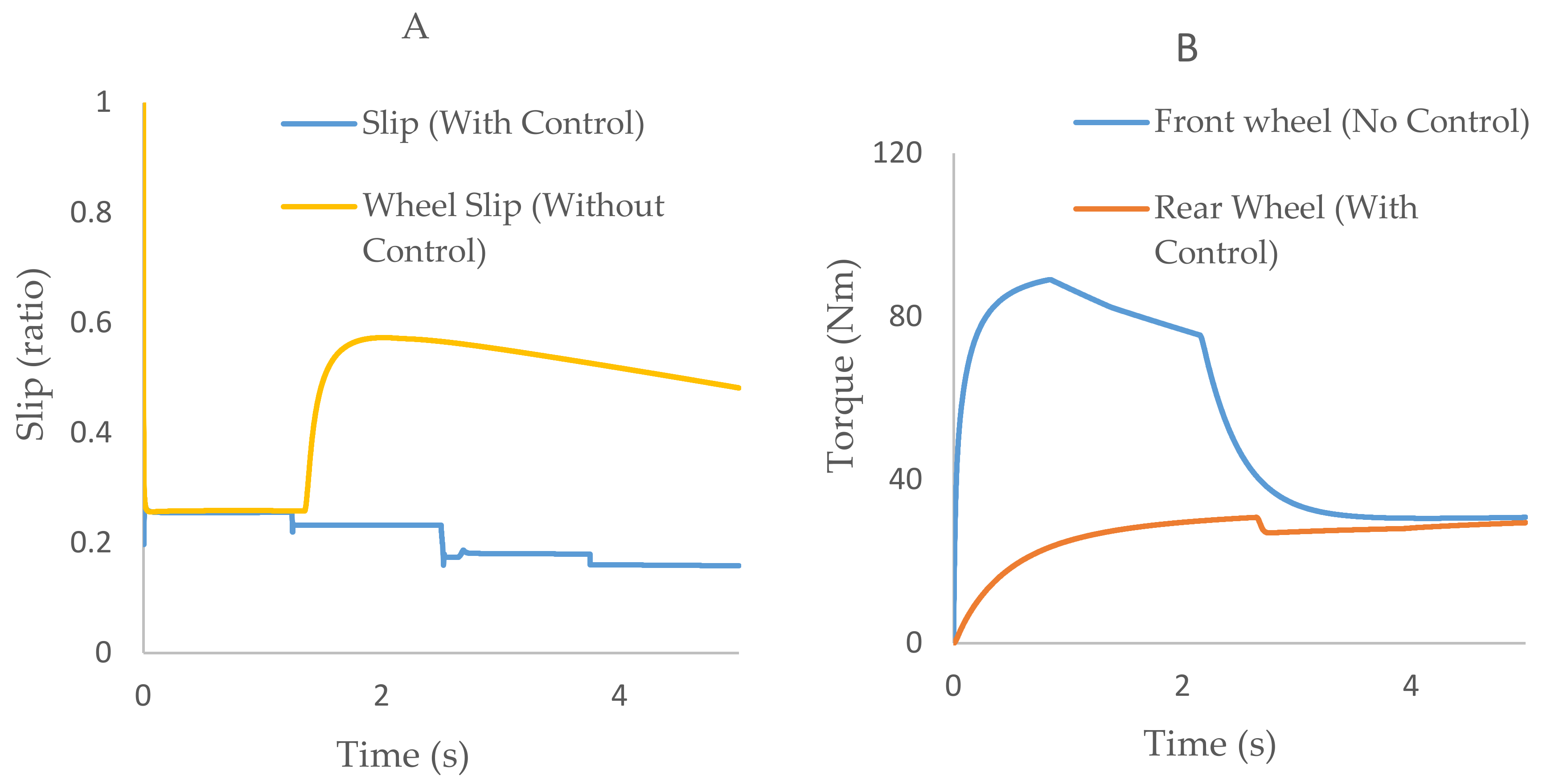
Another simulation was conducted on a variable μ surface; the value of μ was gradually reduced from that of dry concrete surface to wet concrete, ice, and finally snow surface (0.8–0.18); this was to simulate the worst case of μ transition in real field situations. The vehicle model was steadily accelerated in the test from 0 to 5 s by applying a ramp input. Like the previous case, the wheel velocity diverged to more than twice the value of vehicle velocity, as shown in Figure 10A, which resulted in the increased wheel slip (Figure 11A), thereby not accelerating the vehicle significantly.
However, when the traction controller was applied, the slip ratio was regulated within the optimum range. The wheel velocity did not diverge as in the first case (Figure 10A and Figure 11A).
As shown in Figure 11B, the torque supplied by the motor when the traction control was not implemented reached up to 90 Nm before settling down at about 27 Nm. However, when TC was implemented, it increased steadily to a maximum of about 30 Nm, and the fluctuation was less. The increase in torque when TC was not used did not result in increased vehicle velocity, as depicted in Figure 10B, while in the previous instance, it was used up, to increase slip the wheels.
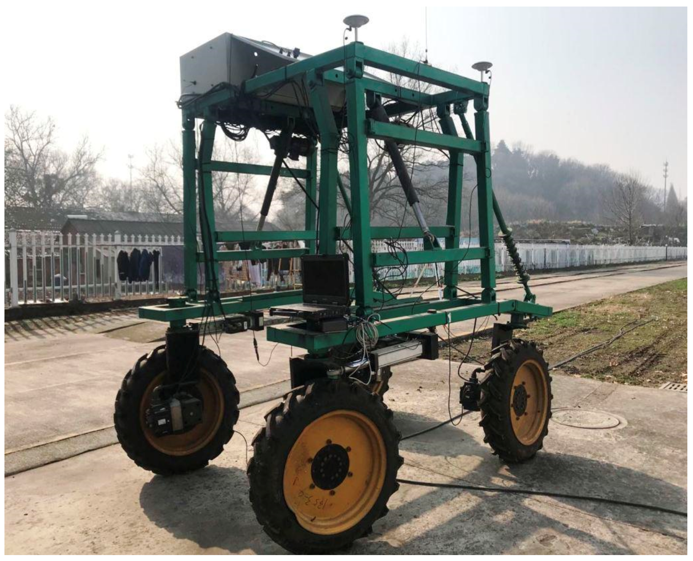
4.3. Field Experiment
In order to verify the performance of the proposed algorithms, experiments were designed and conducted using an experimental platform developed by Nanjing agricultural university (Figure 12), at the Jiangsu Agricultural Machinery testing station. The vehicle was equipped with four in-wheel electric motors, and its parameters were the same as those used during the simulations. The terrain surfaces were dry concrete and moist soil with estimated friction coefficients of 0.8 and 0.2–0.3, respectively.
The velocity and drive torque of each wheel was measured using Panasonic A52 series servo motor driver. The model number and precision of the servo driver were MFME454G1G and 0.1 m/s, respectively. The vehicle velocity and acceleration were measured by P3 Beidou reference station receiver with a speed precision of 0.03 m/s. The control algorithm simulates in Section 3 were converted and uploaded to S7-200 Microcontroller, which is available on the experimental platform. The platform was tested for acceleration on a low μ surface (wet grassy clayey soil surface). Two tests were conducted, one with the traction control engage and the other without engaging the algorithm. In each of the cases, the vehicle was run on a straight line for 35 s at a speed range of about 0–2 m/s. The vehicle was accelerated and decelerated from the beginning to the end of field during the test. The values of wheel torque, slip ratios, wheel speed, and vehicle speed were recorded during the test.
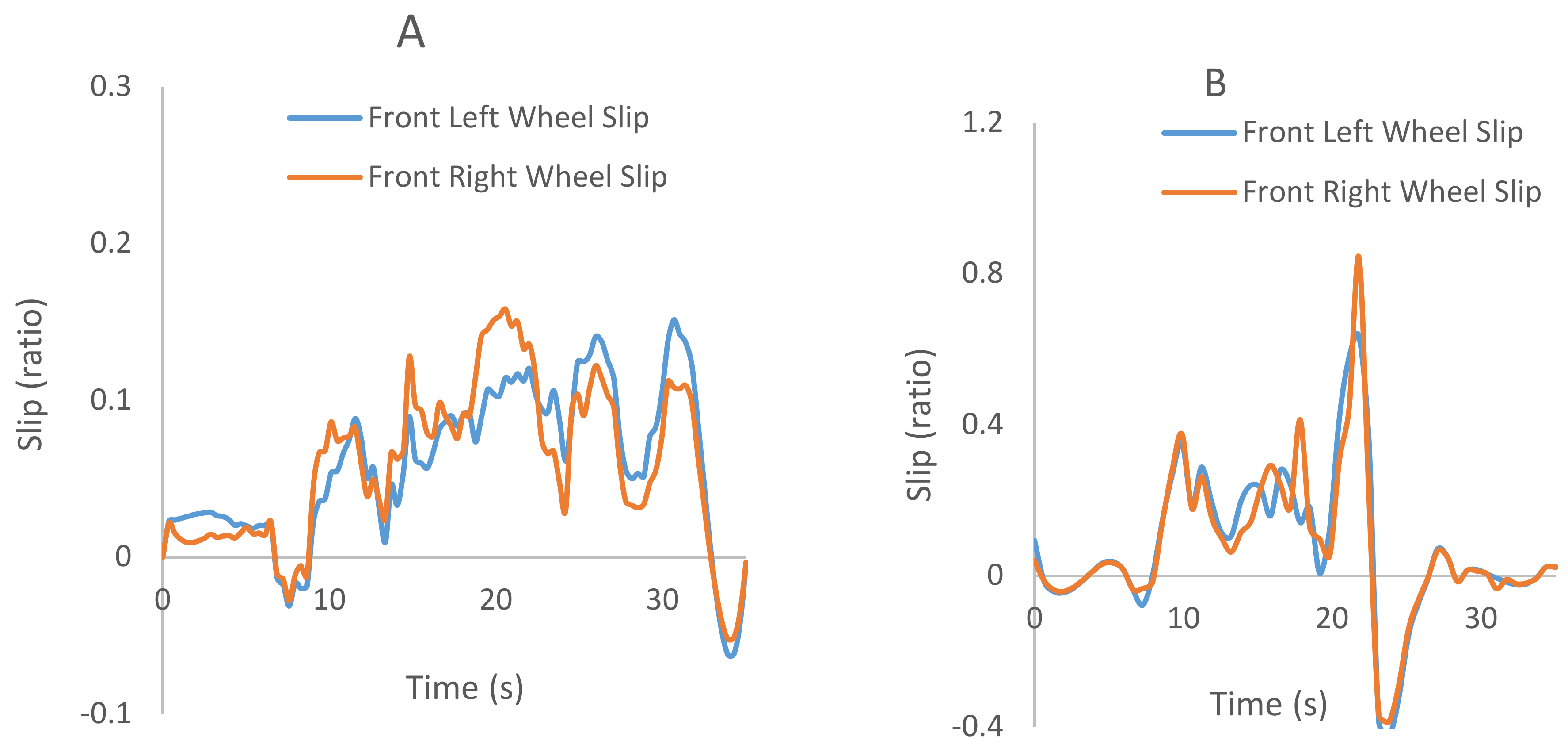
As shown in Figure 13A,B, the slip ratio reached up to 0.8 value when the controller was not engaged, and the value was regulated at less than or equal to 0.15 when the controller was engaged.
By controlling the slip, the wheel speed was maintained close to the vehicle speed as depicted in Figure 14A. In contrast, the wheel speed diverges from the vehicle speed significantly in Figure 14B, during the test without the controller.
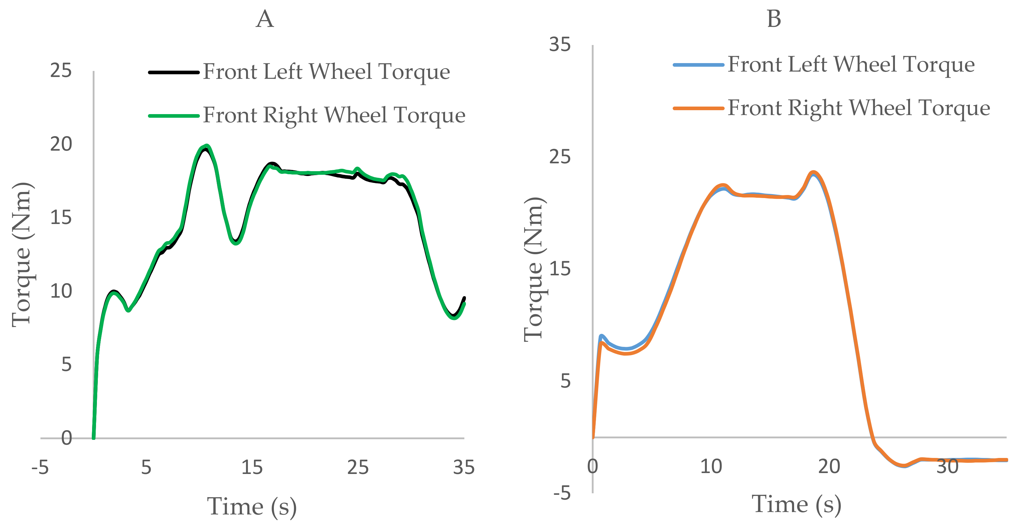
The torque performances of the system are shown in Figure 15; it is observed that the torque delivered in the controlled case is about a maximum value of 19 Nm, while in the uncontrolled case, it reached up to 24 Nm; this indicates that the motor delivered more torque in the uncontrolled test, even though the vehicle accelerated more in the test when the controller was applied. Therefore, the controller assists in reducing torque wastage.
On a general note, comparing the controller’s simulated and field response, a similar trend was observed during acceleration and transition from one surface to another. The controller reduces the torque delivered to the wheels, which decreases the wheel speed, thereby suppressing the slip ratio to a lower value that cannot cause soil disturbance and unnecessary loss of energy. However, it is observed that the controller gave more torque (up to 30 Nm) during the simulation, in comparison to the field test, which was about 19 Nm (Figure 11B and Figure 15A). In both simulation and field tests, the trend of the results for slip ratio, torque, and velocity was similar. It can be observed that at some point in the field test results, the torque and slip ratio were negative; this was due to sudden application of brake while maneuvering the vehicle in the field.
5. Conclusions
The study proposed and developed an efficient and feasible means of estimating an optimum slip that corresponds to maximum traction and low soil disturbances. A robust integral sliding mode control scheme was applied to regulate the slip at the optimum estimated value that guaranteed high traction force. Using an instrumented electric vehicle test platform developed by Nanjing agricultural university, the proposed system was verified to be effective during simulation and field experiments. The controller was able to quickly estimate and track the optimum slip despite the modelling uncertainties and changes in terms of weight on wheels and the rolling resistance. The algorithm assigned an optimal torque to the wheels during acceleration on low μ surfaces, and in the transition from high to low μ surfaces. It suppressed the slip ratio from the non-optimal value of about 0.8 and above, to optimal values of less than 0.2. Therefore, the controller is recommended for use in traction control for maximum traction, reduced soil disturbance, and lower power consumption.
Author Contributions
Conceptualization, I.I.S. and J.Z. (Jun Zhou); methodology, I.I.S., Z.W., C.S., J.Z. (Jianlei Zhao), and Y.W.; software, I.I.S., C.S., and Z.W.; validation, J.Z. (Jun Zhou); investigation, I.I.S., J.Z. (Jianlei Zhao), and Y.W.; resources, J.Z. (Jun Zhou); data curation, J.Z. (Jianlei Zhao) and Y.W.; writing—original draft preparation, I.I.S.; writing—review and editing, C.S., Z.W., J.Z. (Jianlei Zhao), and Y.W.; supervision, J.Z. (Jun Zhou); project administration, J.Z. (Jun Zhou); funding acquisition, J.Z. (Jun Zhou). All authors have read and agreed to the published version of the manuscript.
Funding
This work was financially supported by the national key research and development plan (No. 2016YFD0701003), and the Jiangsu provincial key research and development plan (No. BE2017370).
Institutional Review Board Statement
Not applicable.
Informed Consent Statement
Not applicable.
Data Availability Statement
Not applicable.
Conflicts of Interest
The authors declare no conflict of interest.
Nomenclature
| μ | friction coefficients |
| T | wheel torque |
| r | wheel radius |
| b | wheel with |
| slip ratio | |
| RLS | least square algorithms |
| PI | proportional integral controller |
| GPS | geographical positioning system |
| vertical load acting on the wheel | |
| M | the mass of the vehicle |
| longitudinal acceleration | |
| lateral acceleration | |
| distance from the vehicle center of gravity to the axis that passed through the center of the front wheels | |
| distance from the vehicle center of gravity to the axis that passed through the center of the rear wheels | |
| front and rear wheelbase (equal length) | |
| height of the center of gravity | |
| wheel inertia including motor and reducer | |
| observer gain | |
| wheel torque | |
| DC | direct current voltage |
| ET | electric tractors |
| MTTE | maximum transmissible torque estimation |
| MFC | model following control |
| SVM | support vector machine |
| ANN | artificial neural network |
| Froll | rolling resistance force on wheels |
| longitudinal tire-road friction force | |
| lateral tire-road friction force | |
| vehicle longitudinal velocity | |
| wheel rotational velocity | |
| sliding mode control | |
| rolling resistance coefficient | |
| Subscripts | |
| fl | front left |
| fr | front right |
| rl | rear left |
| rr | rear right |
References
- Ehsani, M.; Gao, Y.; Longo, S.; Ebrahimi, K. Modern Electric, Hybrid Electric, and Fuel Cell Vehicles; CRC Press: Boca Raton, FL, USA, 2018. [Google Scholar]
- Hori, Y.; Toyoda, Y.; Tsuruoka, Y. Traction control of electric vehicle: Basic experimental results using the test EV “UOT Electric March”. IEEE Trans. Ind. Appl. 1998, 34, 1131–1138. [Google Scholar] [CrossRef]
- Zhou, X.; Zhou, J.; Wang, Z.; Yang, L.; Yu, M. The control of high-clearance electric vehicles based on pavement parameter estimations. Adv. Mech. Eng. 2018, 10, 1687814018786377. [Google Scholar] [CrossRef]
- Jia, C.; Qiao, W.; Qu, L. Numerical Methods for Optimal Control of Hybrid Electric Agricultural Tractors. In Proceedings of the 2019 IEEE Transportation Electrification Conference and Expo (ITEC), Novi, MI, USA, 19–21 June 2019; pp. 1–6. [Google Scholar]
- Ding, Z.; Li, B. Design and Analysis of the Suspension for Electric Tractor. IOP Conf. Ser. Mater. Sci. Eng. 2019, 493, 012077. [Google Scholar] [CrossRef]
- Melo, R.R.; Antunes, F.L.; Daher, S.; Vogt, H.H.; Albiero, D.; Tofoli, F.L. Conception of an electric propulsion system for a 9 kW electric tractor suitable for family farming. IET Electr. Power Appl. 2019, 13, 1993–2004. [Google Scholar] [CrossRef]
- Li, T.; Xie, B.; Wang, R. Design and experiments of electronic steer-by-wire system in electric tractor. IOP Conf. Ser. Earth Environ. Sci. 2019, 252, 032108. [Google Scholar] [CrossRef] [Green Version]
- Sunusi, I.I.; Zhou, J.; Wang, Z.Z.; Sun, C.; Ibrahim, I.E.; Opiyo, S.; Korohou, T.; Soomro, S.A.; Alhaji Sale, N.; Olanrewaju, T.O. Intelligent tractors: Review of online traction control process. Comput. Electron. Agric. 2020, 170, 105176. [Google Scholar] [CrossRef]
- Cairns, E.J.; Albertus, P. Batteries for Electric and Hybrid-Electric Vehicles. Annu. Rev. Chem. Biomol. Eng. 2010, 1, 299–320. [Google Scholar] [CrossRef]
- Burke, A.F. Batteries and Ultracapacitors for Electric, Hybrid, and Fuel Cell Vehicles. Proc. IEEE 2007, 95, 806–820. [Google Scholar] [CrossRef]
- Gerssen-Gondelach, S.J.; Faaij, A.P.C. Performance of batteries for electric vehicles on short and longer term. J. Power Sour. 2012, 212, 111–129. [Google Scholar] [CrossRef]
- Gandoman, F.H.; Jaguemont, J.; Goutam, S.; Gopalakrishnan, R.; Firouz, Y.; Kalogiannis, T.; Omar, N.; Van Mierlo, J. Concept of reliability and safety assessment of lithium-ion batteries in electric vehicles: Basics, progress, and challenges. Appl. Energy 2019, 251, 113343. [Google Scholar] [CrossRef]
- Nykvist, B.; Sprei, F.; Nilsson, M. Assessing the progress toward lower priced long range battery electric vehicles. Energy Policy 2019, 124, 144–155. [Google Scholar] [CrossRef]
- Kuntanapreeda, S. Traction control of electric vehicles using sliding-mode controller with tractive force observer. Int. J. Veh. Technol. 2014, 2014, 829097. [Google Scholar] [CrossRef] [Green Version]
- Nam, K.; Hori, Y.; Lee, C.J.E. Wheel slip control for improving traction-ability and energy efficiency of a personal electric vehicle. Energies 2015, 8, 6820–6840. [Google Scholar] [CrossRef] [Green Version]
- Khatun, P.; Bingham, C.M.; Schofield, N.; Mellor, P.H. Application of fuzzy control algorithms for electric vehicle antilock braking/traction control systems. IEEE Trans. Ind. Appl. 2003, 52, 1356–1364. [Google Scholar] [CrossRef]
- Fuse, H.; Fujimoto, H. Driving Force Controller with Variable Slip Ratio Limiter for Electric Vehicle Considering Lateral Slip Based on Brush Model. In Proceedings of the 2019 IEEE Vehicle Power and Propulsion Conference (VPPC), Hanoi, Vietnam, 14–17 October 2019; pp. 1–6. [Google Scholar]
- Gonzalez, R.; Apostolopoulos, D.; Iagnemma, K. Improving rover mobility through traction control: Simulating rovers on the Moon. Auton. Robot. 2019, 43, 1977–1988. [Google Scholar] [CrossRef]
- König, L.; Schindele, F.; Zimmermann, A. ITC–Integrated traction control for sports car applications. In 19. Internationales Stuttgarter Symposium; Springer: Berlin/Heidelberg, Germany, 2019; pp. 457–470. [Google Scholar]
- Dogan, D.; Boyraz, P. Smart Traction Control Systems for Electric Vehicles Using Acoustic Road-Type Estimation. IEEE Trans. Intell. Veh. 2019, 4, 486–496. [Google Scholar] [CrossRef]
- Ma, Y.; Zhao, J.; Zhao, H.; Lu, C.; Chen, H. MPC-Based Slip Ratio Control for Electric Vehicle Considering Road Roughness. IEEE Access 2019, 7, 52405–52413. [Google Scholar] [CrossRef]
- Yin, D.; Sun, N.; Hu, J. A Wheel Slip Control Approach Integrated with Electronic Stability Control for Decentralized Drive Electric Vehicles. IEEE Trans. Ind. Inform. 2019, 15, 2244–2252. [Google Scholar] [CrossRef]
- Liu, H.H.S.; Pang, G.K.H. Accelerometer for mobile robot positioning. IEEE Trans. Ind. Appl. 2001, 37, 812–819. [Google Scholar] [CrossRef]
- Pang, G.; Liu, H. Evaluation of a Low-cost MEMS Accelerometer for Distance Measurement. J. Intell. Robot. Syst. 2001, 30, 249–265. [Google Scholar] [CrossRef]
- Antonello, R.; Ito, K.; Oboe, R. Acceleration Measurement Drift Rejection in Motion Control Systems by Augmented-State Kinematic Kalman Filter. IEEE Trans. Ind. Electron. 2016, 63, 1953–1961. [Google Scholar] [CrossRef]
- Rock, K.L.; Beiker, S.A.; Laws, S.; Gerdes, J.C. Validating GPS Based Measurements for Vehicle Control. In Proceedings of the ASME 2005 International Mechanical Engineering Congress and Exposition, Orlando, FL, USA, 5–11 November 2005; pp. 583–592. [Google Scholar]
- Bae, H.S.; Ryu, J.; Gerdes, J.C. Road grade and vehicle parameter estimation for longitudinal control using GPS. In Proceedings of the IEEE Conference on Intelligent Transportation Systems, Oakland, CA, USA, 25–29 August 2001; pp. 25–29. [Google Scholar]
- Itou, K.; Fujita, T.; Shirato, R.; Akiba, T. A Study of Novel Traction Control Method for Electric Motor Driven Vehicle; The Automotive Research Association of India: Pune, India, 2009. [Google Scholar]
- Okano, T.; Tai Chien, H.; Inoue, T.; Uchida, T.; Shin-Ichiro, S.; Hori, Y. Vehicle stability improvement based on MFC independently installed on 4 Wheels-basic experiments using “UOT Electric March II”. In Proceedings of the Power Conversion Conference-Osaka 2002 (Cat. No.02TH8579), Osaka, Japan, 2–5 April 2002; Volume 2, pp. 582–587. [Google Scholar]
- Ewin, N.J.; Howey, D.A.; McCulloch, M.D. MTTE-Based traction control for directional stability on mixed-μ roads. In IET Conference Proceedings; Institution of Engineering and Technology: London, UK, 2013; pp. 74–79. [Google Scholar]
- Hu, J.-S.; Yin, D.; Hori, Y. Electric Vehicle Traction Contro-A New MTTE Approach with PI Observer. IFAC Proc. 2009, 42, 137–142. [Google Scholar] [CrossRef]
- Song, Z.; Li, J.; Xu, L.; Ouyang, M. Traction Control System for EV Based on Modified Maximum Transmissible Torque Estimation. In Proceedings of the 2013 IEEE Vehicle Power and Propulsion Conference (VPPC), Beijing, China, 15–18 October 2013; pp. 1–7. [Google Scholar]
- Khatun, P.; Bingham, C.; Mellor, P. Comparison of Control Methods for Electric Vehicle Antilock Braking/Traction Control Systems; SAE Technical Paper; SAE International: Warrendale, PA, USA, 2001; ISSN 0148–7191. [Google Scholar] [CrossRef]
- Kataoka, H.; Sado, H.; Sakai, I.; Hori, Y. Optimal slip ratio estimator for traction control system of electric vehicle based on fuzzy inference. Electr. Eng. Jpn. 2001, 135, 56–63. [Google Scholar] [CrossRef]
- Masino, J.; Pinay, J.; Reischl, M.; Gauterin, F.J.A.A. Road surface prediction from acoustical measurements in the tire cavity using support vector machine. Appl. Acoust. 2017, 125, 41–48. [Google Scholar] [CrossRef]
- Acosta, M.; Kanarachos, S.; Blundell, M.J.A.S. Road friction virtual sensing: A review of estimation techniques with emphasis on low excitation approaches. Appl. Acoust. 2017, 7, 1230. [Google Scholar] [CrossRef] [Green Version]
- Li, L.; Li, H.; Zhang, X.; He, L.; Song, J. Real-time tire parameters observer for vehicle dynamics stability control. Chin. J. Mech. Eng. 2010, 23, 620–626. [Google Scholar] [CrossRef]
- Geist, M.; Pietquin, O. Statistically linearized recursive least squares. In Proceedings of the 2010 IEEE International Workshop on Machine Learning for Signal Processing, Kittilä, Finland, 29 August–1 September 2010; pp. 272–276. [Google Scholar]
- Rhode, S.; Gauterin, F. Online estimation of vehicle driving resistance parameters with recursive least squares and recursive total least squares. In Proceedings of the 2013 IEEE Intelligent Vehicles Symposium (IV), Gold Coast, Australia, 23–26 June 2013; pp. 269–276. [Google Scholar]
- Akbari, A.; Lohmann, B. Multi-Objective H∞/GH2 Preview Control of Active Vehicle Suspensions. Ph.D. Thesis, Technische Universität München, München, Germany, 2009. [Google Scholar]
- Farroni, F.; Russo, M.; Russo, R.; Terzo, M.; Timpone, F. A combined use of phase plane and handling diagram method to study the influence of tyre and vehicle characteristics on stability. Int. J. Veh. Mech. Mobil. 2013, 51, 1265–1285. [Google Scholar] [CrossRef]
- Bucolo, M.; Buscarino, A.; Famoso, C.; Fortuna, L.; Frasca, M. Control of imperfect dynamical systems. Nonlinear Dyn. 2019, 98, 2989–2999. [Google Scholar] [CrossRef]
- Andersen, M.H.; Jensen, H.-C.B. Design of Slip-based Active Braking and Traction Control System for the Electric Vehicle QBEAK. Master’s Thesis, Aalborg University, Aalborg Øst, Danmark, 2012. [Google Scholar]
- Matuško, J.; Petrović, I.; Perić, N. Neural network based tire/road friction force estimation. Eng. Appl. Artif. Intell. 2008, 21, 442–456. [Google Scholar] [CrossRef]
- Wang, R.; Wang, J. Tire–road friction coefficient and tire cornering stiffness estimation based on longitudinal tire force difference generation. Control. Eng. Pract. 2013, 21, 65–75. [Google Scholar] [CrossRef]
- Ray, L.R. Nonlinear Tire Force Estimation and Road Friction Identification: Simulation and Experiments. Automatica 1997, 33, 1819–1833. [Google Scholar] [CrossRef]
- Feng, Y.; Chen, H.; Zhao, H.; Zhou, H. Road tire friction coefficient estimation for four wheel drive electric vehicle based on moving optimal estimation strategy. Mech. Syst. Signal Process. 2019, 139, 106416. [Google Scholar] [CrossRef]
- Patra, N.; Datta, K. Observer Based Road-Tire Friction Estimation for Slip Control of Braking System. Procedia Eng. 2012, 38, 1566–1574. [Google Scholar] [CrossRef] [Green Version]
- Liu, Y.H.; Li, T.; Yang, Y.Y.; Ji, X.W.; Wu, J. Estimation of tire-road friction coefficient based on combined APF-IEKF and iteration algorithm. Mech. Syst. Signal Process. 2017, 88, 25–35. [Google Scholar] [CrossRef]
- Jin, X.; Yin, G.; Chen, N. Advanced Estimation Techniques for Vehicle System Dynamic State: A Survey. Sensors 2019, 19, 4289. [Google Scholar] [CrossRef] [Green Version]
- Ferrara, A. Sliding Mode Control of Vehicle Dynamics; Institution of Engineering and Technology: London, UK, 2017. [Google Scholar]
- Slotine, J.-J.E.; Li, W. Applied Nonlinear Control; Prentice Hall Englewood Cliffs, NJ: Fort Wayne, IN, USA, 1991; Volume 199. [Google Scholar]
- Gómez Fernández, J. A Vehicle Dynamics Model for Driving Simulators. Master’s Thesis, Chalmers University of Technology, Göteborg, Sweden, 2012. [Google Scholar]
- Utkin, V.; Guldner, J.; Shijun, M. Sliding Mode Control in Electro-Mechanical Systems; CRC Press: Boca Raton, FL, USA, 1999; Volume 34. [Google Scholar]
- Pacejka, H. Tire and Vehicle Dynamics; Elsevier: Amsterdam, The Netherlands, 2005. [Google Scholar]
- Svendenius, J. Tire Modeling and Friction Estimation. Ph.D. Thesis, Department of Automatic Control, Lund University, Lund, Sweden, 2007. [Google Scholar]
- Li, Q.; Liu, L.; Yuan, X. Model Predictive Controller-Based Optimal Slip Ratio Control System for Distributed Driver Electric Vehicle. J. Math. Probl. Eng. 2020, 2020, 8086590. [Google Scholar] [CrossRef]
- Bian, M.; Chen, L.; Luo, Y.; Li, K. Research on maximum road adhesion coefficient estimation for distributed drive electric vehicle. In Proceedings of the 2013 International Conference on Mechanical and Automation Engineering, Jiujang, China, 21–23 July 2013; pp. 90–94. [Google Scholar]
- Cui, G.; Dou, J.; Li, S.; Zhao, X.; Lu, X.; Yu, Z. Slip control of electric vehicle based on tire-road friction coefficient estimation. Math. Probl. Eng. 2017, 2017, 1–8. [Google Scholar] [CrossRef] [Green Version]
- Phillips, C.L.; Harbor, R.D. Feedback Control Systems; Prentice Hall: Upper Saddle River, NJ, USA, 2000; Volume 581. [Google Scholar]
Figure 1.
Free body diagram of the vehicle: (A) view from the top and (B) view from the side.

Figure 2.
Free body diagram of one wheel.

Figure 3.
Slip ratio versus friction coefficient.


Figure 5.
Diagram of the observer and sliding mode controller.

Figure 6.
Estimation of optimum friction coefficient.

Figure 7.
Controller robustness to disturbances: (A) RRC variations and (B) weight variations.

Figure 8.
Velocity performance (A) without control and (B) with control.

Figure 9.
Controller performance in low μ terrain: (A) slip variation and (B) torque variation.

Figure 10.
Velocity performances (A) without control and (B) with control.

Figure 11.
Test performance for μ transition: (A) slip variation and (B) torque variation.

Figure 12.
Electric vehicle testing platform in the field.

Figure 13.
Slip ratio performances (A) with control and (B) without control.

Figure 14.
Speed performances (A) with control and (B) without control.

Figure 15.
Torque performances (A) with control and (B) without control.


Table 1.
Parameters of road surface adhesion coefficient [57].
Table 1.
Parameters of road surface adhesion coefficient [57].
| Road Surface | |||
|---|---|---|---|
| Dry asphalt | 1.28 | 23.99 | 0.52 |
| Wet asphalt | 0.86 | 33.82 | 0.35 |
| Wet pebbles | 0.40 | 33.71 | 0.12 |
| Snow | 0.19 | 94.13 | 0.06 |
| Ice | 0.05 | 306.4 | 0.001 |
Table 2.
Parameters of the vehicle’s major components.
| Parameters | Value |
|---|---|
| Vehicle weight (kg) | 1200 |
| Width (m) | 2.3 |
| Height (m) | 2.5 |
| Wheelbase (m) | 2.2 |
| Ground clearance (m) | 2.2 |
| Rated power (kW) | 4.5 |
| Rated torque (Nm) | 21.5 |
| Maximum torque (Nm) | 54.9 |
| Rated speed (rpm) | 2000 |
| Maximum speed (rpm) | 3000 |
| Motor speed reduction ratio | 32:1 |
| Total wheel inertia (Kgms2) | 1.95 |
| Wheel radius (M) | 0.326 |
| Center of Gravity (CG) | 1.1 |
Table 3.
Bounded model parameters.
| Parameter/Value | Minimum Value | Estimate | Maximum Value | Maximum Deviation |
|---|---|---|---|---|
| Mass on the wheels (kg) | 200 | 375 | 600 | 225 |
| Rolling resistance coefficient () | 0.1 | 0.15 | 0.2 | 0.05 |
Publisher’s Note: MDPI stays neutral with regard to jurisdictional claims in published maps and institutional affiliations. |
© 2021 by the authors. Licensee MDPI, Basel, Switzerland. This article is an open access article distributed under the terms and conditions of the Creative Commons Attribution (CC BY) license (https://creativecommons.org/licenses/by/4.0/).
Share and Cite
MDPI and ACS Style
Sunusi, I.I.; Zhou, J.; Sun, C.; Wang, Z.; Zhao, J.; Wu, Y. Development of Online Adaptive Traction Control for Electric Robotic Tractors. Energies 2021, 14, 3394. https://0-doi-org.brum.beds.ac.uk/10.3390/en14123394
AMA Style
Sunusi II, Zhou J, Sun C, Wang Z, Zhao J, Wu Y. Development of Online Adaptive Traction Control for Electric Robotic Tractors. Energies. 2021; 14(12):3394. https://0-doi-org.brum.beds.ac.uk/10.3390/en14123394
Chicago/Turabian StyleSunusi, Idris Idris, Jun Zhou, Chenyang Sun, Zhenzhen Wang, Jianlei Zhao, and Yongshuan Wu. 2021. "Development of Online Adaptive Traction Control for Electric Robotic Tractors" Energies 14, no. 12: 3394. https://0-doi-org.brum.beds.ac.uk/10.3390/en14123394
Note that from the first issue of 2016, this journal uses article numbers instead of page numbers. See further details here.