Discovery of Dynamic Two-Phase Flow in Porous Media Using Two-Dimensional Multiphase Lattice Boltzmann Simulation

Abstract

The dynamic two-phase flow in porous media was theoretically developed based on mass, momentum conservation, and fundamental constitutive relationships for simulating immiscible fluid-fluid retention behavior and seepage in the natural geomaterial. The simulation of transient two-phase flow seepage is, therefore, dependent on both the hydraulic boundaries applied and the immiscible fluid-fluid retention behavior experimentally measured. Many previous studies manifested the velocity-dependent capillary pressure–saturation relationship (P_c-S) and relative permeability (K_r-S). However, those works were experimentally conducted on a continuum scale. To discover the dynamic effects from the microscale, the Computational Fluid Dynamic (CFD) is usually adopted as a novel method. Compared to the conventional CFD methods solving Naiver–Stokes (NS) equations incorporated with the fluid phase separation schemes, the two-phase Lattice Boltzmann Method (LBM) can generate the immiscible fluid-fluid interface using the fluid-fluid/solid interactions at a microscale. Therefore, the Shan–Chen multiphase multicomponent LBM was conducted in this study to simulate the transient two-phase flow in porous media. The simulation outputs demonstrate a preferential flow path in porous media after the non-wetting phase fluid is injected until, finally, the void space is fully occupied by the non-wetting phase fluid. In addition, the inter-relationships for each pair of continuum state variables for a Representative Elementary Volume (REV) of porous media were analyzed for further exploring the dynamic nonequilibrium effects. On one hand, the simulating outcomes reconfirmed previous findings that the dynamic effects are dependent on both the transient seepage velocity and interfacial area dynamics. Nevertheless, in comparison to many previous experimental studies showing the various distances between the parallelly dynamic and static P_c-S relationships by applying various constant flux boundary conditions, this study is the first contribution showing the P_c-S striking into the nonequilibrium condition to yield dynamic nonequilibrium effects and finally returning to the equilibrium static P_c-S by applying various pressure boundary conditions. On the other hand, the flow regimes and relative permeability were discussed with this simulating results in regards to the appropriateness of neglecting inertial effects (both accelerating and convective) in multiphase hydrodynamics for a highly pervious porous media. Based on those research findings, the two-phase LBM can be demonstrated to be a powerful tool for investigating dynamic nonequilibrium effects for transient multiphase flow in porous media from the microscale to the REV scale. Finally, future investigations were proposed with discussions on the limitations of this numerical modeling method.

1. Introduction

Immiscible two-phase flow seepage in porous media is a physical process, which often appears in environmental, geotechnical, and petroleum engineering. The conventional theory for simulating this physical phenomenon can be summarized in two types of formulation: (1) for the Enhancement of Oil Recovery (EOR) in petroleum engineering, the theory consists of two sets of mass and momentum conservation equations (continuity equations and Darcy’s law) for both wetting and non-wetting fluid phase, and the experimental determination of capillary pressure/relative permeability–saturation curves (P_c-S/K_r-S) [1,2]; (2) for the environmental and geotechnical engineering, the soil suction is usually taken as a negative pore water pressure, due to setting atmosphere pressure as reference zero for air. In this way, the P_c-S can be transformed as the Soil Water Retention Curve (SWRC). Thus, the entire theory of two-phase flow seepage for EOR can be simplified to only one set of continuity equations and Darcy’s law, which composed the Richards equation [3] for simulating soil moisture transport in unsaturated soil [4,5]. Despite the difference in the constant non-wetting phase pressure, both are exactly in the same theoretical framework. Thus, the prediction given by solving this theory should be dependent on the experimentally derived P_c-S/K_r-S curves and hydraulic boundary conditions applied along each side of simulating domain. On the other hand, from the mechanical perspective of unsaturated soil, the cohesion and consolidation of unsaturated soil can also be varied by soil suction and moisture content. Whether the theory can accurately approximate the soil water/suction will have further determined impacts on the mechanical behavior of unsaturated soil regarding shear strength and stress–suction–strain constitutive relationships [6,7,8,9]. There are also other concerns about the application of unsaturated soil for the limit equilibrium method in regards to geotechnical design [4,5]. Therefore, the measurement of the P_c-S curve or SWRC critically determines the prediction of the hydro-mechanical behavior of unsaturated soil.

A few decades ago, before introducing the soil water retention concept into geotechnical engineering, many soil scientists already uncovered the dynamic effects in Pc-S curves [10,11,12,13,14]. In general, according to their experimental results, compared to the static P_c-S measured by the conventional methods adopting static datasets, the dynamic P_c-S curves yielded under transient flow conditions manifest a higher suction for drainage and a lower suction for imbibition. Additionally, the deviation between static and dynamic SWRC can be enlarged by increasing the flow velocity or variation of saturation, and this was later defined as the dynamic effects in P_c-S curves or SWRC by Hassanizadeh et al. [15]. In the same era, three new advanced theories were simultaneously composed of the modeling transient multiphase flow seepage without the assumption of instantaneous equilibrium for P_c-S [16,17,18]. However, due to difficulties in measuring new parameters involved in those theories, the comprehensive validation of theories is still currently under development [19,20,21,22,23,24,25,26,27,28,29,30,31,32,33,34,35]. Nevertheless, these experimental studies had their natural constraints in terms of continuum scale and boundary effects, because the soil suction and moisture content can only be detected using electrical/dielectric sensors on a soil column, and the ceramic disk with high air entry value under soil specimen potentially slow down the two-phase flow seepage velocity, which might be different from the natural transient two-phase flow seepage velocity. A few studies on microscale physical models can provide both observations from the microscale behavior to the state variables in the continuum scale [36,37,38,39,40]. In comparison to those physical experiments, the Computational Fluid Dynamic (CFD) simulation could be another useful approach to investigate the transient multiphase flow seepage.

In recent decades, many CFD simulations have been implemented to study two immiscible phase fluids seeping through porous media. The simulating methods can be summarized into two main categories in terms of fluid phase separation methods: (1) solving the Naiver–Stokes (NS) equations with a Young–Laplace equation and generating an interface using the Volume of Fluid (VOF) or Level-Set (LS) on the level of control volume [40,41,42,43,44]; (2) solving the Lattice Boltzmann equations and generating an interface on the microscale [45,46,47,48,49,50,51,52]. As the Young–Laplace equation is a static expression of the interface and can only be applied to simulated steady-state multiphase flow in porous media [44,53], Ferrari and Lunati [41] further developed conventional VOF methods incorporated with Helmholtz free energy instead of simply applying the static Young–Laplace equation to simulate the interface dynamics. With this novel numerical method, the internal effects and instability on the meniscus and dynamic effects in capillary flow and P_c-S can be investigated [40,41,42,43]. However, this method has limitations on detecting interfaces under low-velocity conditions due to the dependence of velocity for the determination of the meniscus [40].

Compared to this numerical method, the Shan–Chen LBM (SC-LBM) applies three fundamental interactive forces between each pair of three phases (wetting fluid, non-wetting fluid, and solid) to generate the fluid-fluid interfaces and hydrophobicity/hydrophilicity in their density domain. As the SC-LBM owns the fundamental physics in generating the immiscible phase phenomenon, it was usually applied to replicate the static capillary behavior [45,46,47,54] and to study static/steady-state P_c-S [48,50,55,56,57,58,59,60] even with hysteresis issue [61] and interface [52,58,59,60] as well as steady-state K_r-S relationships [58,59,62]. However, only a few studies using SC-LBM have been presented for investigating dynamic effects in a capillary tube [49], porous media [27,34,63,64,65], and sandstones [66,67]. Porter, Schaap, and Wildenschild [63] studied the dynamic effects in capillary pressure and P_c-S using SC-LBM and the dynamic P_c-S relationships showed high fluctuations which are not very inconsistent with experimental findings. Galindo-Torres, Scheuermann, Li, Pedroso, and Williams [64] and Scheuermann, Galindo-Torres, Pedroso, Williams, and Li [27] also investigated the dynamic effects in hysteresis SWRC using SC-LBM and defined such dynamic hysteresis SWRC as a so-called “hydraulic ratcheting” in unsaturated soil. However, as the simulation was carried out using single component multiphase SC-LBM, the water potential was not determined in capillary pressure or soil suction but a water potential in elevation head for an original purpose of studying groundwater table dynamics in consideration of capillary fringe. Recent studies of the dynamic effects in P_c-S relationships using SC-LBM can be sourced from Yan, Li, Bore, Galindo-Torres, Scheuermann, and Li [65] and Yan, Bore, Galindo-Torres, Scheuermann, Li and Schlaeger [34], in which the dynamic P_c-S relationships with interface dynamics were successfully generated using multicomponent multiphase SC-LBM. Additionally, Tang, Zhan, Ma, and Lu [66] and Cao, Tang, Zhang, Tang, and Lu [67] applied SC-LBM to the investigations of dynamic P_c-S in sandstones merely on transient drainage paths. Nevertheless, those studies were still at the initial stage and have not been deeply investigated in consideration of various boundary conditions and hydraulic loading paths.

With the aim to further explore the dynamic two-phase flow in porous media, the Shan–Chen multiphase multicomponent Lattice Boltzmann Method (SC-LBM) was adopted in this study. Taking the advantages of SC-LBM, the fast one-step in/outflow numerical experiments were implemented by varying the in/output pressure along the top and bottom boundaries to replicate the pressure cell experiment or in another description as a single REV in a vertical profile of porous media. Thus, the dynamic response of capillary pressure (P_c), saturation (S), interfacial area (a_nw), and flux (q) can be instantaneously determined from microscale immiscible phase fluid densities and velocities. The resulting analysis is presented with a discussion on the significances of novel findings from a physical perspective. It motivates and orientates future investigation using this numerical method. Additionally, the potential limitations of this LBM are discussed for the improvement of this numerical method.

2. Numerical Methodology

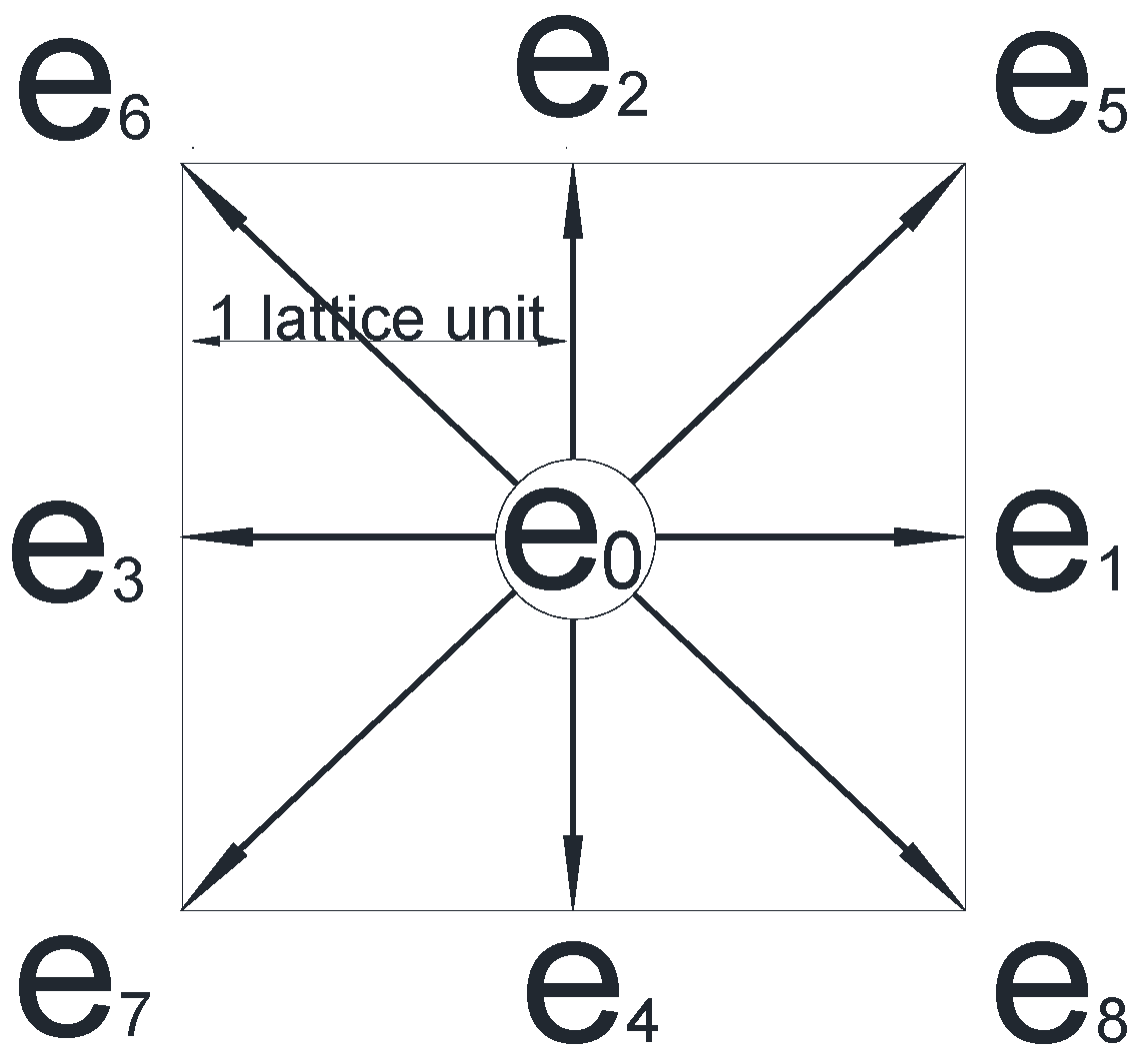
2.1. Shan–Chen Multiphase Multicomponent Lattice Boltzmann Method

The Lattice Boltzmann Method (LBM) is a CFD method solving the Boltzmann equation on a discretized density and velocity field. As the simulating domain consists of many squares for 2D, the density and velocity can be calculated on each node knitted by a lattice grid. The original Boltzmann equation is written in continuum form:

$$f_i\left(x+dx,\mathbf{p}+d\mathbf{p},t+dt\right)d\mathbf{x}d\mathbf{p}-f_i\left(x,\mathbf{p},t\right)d\mathbf{x}d\mathbf{p}=[{\mathsf{\Gamma }}^{(+)}-{\mathsf{\Gamma }}^{(-)}]d\mathbf{x}d\mathbf{p}dt$$

(1)

where f is a probability function for finding a molecule i in a given location; x, p, and t are, respectively, the location in a coordinate, momentum of molecule i, and the time; and Γ is the number of molecules either arriving in (+) or leaving out (−) of the given location [68]. In principle, Equation (1) demonstrates that the streaming of fluid molecules in a given space is dependent on the collision process. In order to numerically solve this equation, it is further discretized in a square (2D) lattice domain as:

$$\stackrel{\mathrm{Streaming}}{\overbrace{f_i\left(x+e_i\Delta t,t+\Delta t\right)-f_i\left(x,t\right)}}=\frac{\stackrel{\mathrm{Collision}}{\overbrace{\left[f_i{}^{eq}\left(x,t\right)-f_i\left(x,t\right)\right]}}}{\tau }$$

(2)

where f_i^eq is the equilibrium distribution function and τ is the characteristic relaxation time. In this study, the two-dimensional discretization scheme (D2Q9) is applied, and a schematic plot is shown in Figure 1.

On the left-hand side of Equation (2), to define the macroscopic velocity u and density ρ for each node i, the summation of velocity and density around node i should be applied as follows:

$$\rho ={\displaystyle \sum _{i=0}^8{f}_i}$$

(3)

$$u=\frac{{\displaystyle \sum _{i=0}^8{f}_i{e}_i}}{\rho }$$

(4)

As the velocity u needs summation of momentum surrounding the origin node, according to Figure 1, the discrete velocities are calculated by:

$$\begin{array}{l}{e}_0=(0,0),\\ e_i=c(\cos (\frac{\pi (i-1)}{2}),\sin (\frac{\pi (i-1)}{2})),i=1,2,3,4\\ e_i=\sqrt{2}c(\cos (\frac{\pi (i-3.5)}{2}),\sin (\frac{\pi (i-3.5)}{2})),i=5,6,7,8\end{array}$$

(5)

where c is the basic speed of lattice, defined as one lattice unit length (lu, marked in Figure 1) per lattice time step (ts), i.e., one lu/ts.

On the right-hand side of Equation (2), to determine the collision process, the equilibrium probability function f_i^eq has to be defined. For simulating single and multiphase fluid, the Naiver–Stokes (NS) equation has to be recovered by applying Bhatnagar–Gross–Krook (BGK) approximation, derived from the Taylor series of the Maxwell distribution function [68]:

$$f_i^{eq}=\stackrel{\mathrm{Bhatnagar}-\mathrm{Gross}-\mathrm{Krook}\left(\mathrm{BGK}\right)\mathrm{approximation}\mathrm{of}{f}_i^{eq}}{\overbrace{w_i\rho \left(1+3\frac{e_i\cdot u}{C}+4.5\frac{{(e\cdot u)}^2}{C^4}-1.5\frac{u^2}{C^2}\right)}}$$

(6)

in which there is a need for weight factors (w_i) for each velocity, according to the D2Q9 scheme in Figure 1, defined as:

$$\begin{array}{l}{w}_0=\frac{4}{9},\\ w_i=\frac{1}{9},i=1,2,3,4,\\ w_i=\frac{1}{36},i=5,6,7,8.\end{array}$$

(7)

The characteristic relaxation time τ strongly dominates the numerical stability of the LBM solver. In LBM, it is dependent on the kinematic viscosity of fluid (ν) by:

$$\upsilon =c_s{}^2\Delta \mathrm{t}(\tau -0.5)$$

(8)

where c_s is the sound speed of the lattice (3^−0.5c, lattice basic speed c = Δx/Δt = 1, Δx = 1, Δt = 1). The stability of the LBM numerical solver is dominated by τ, which should be at least above 0.5 to give a physical viscosity in a positive value. Previous experience shows that it generates an unstable solution if τ is close to 0.5, so to be safe, this value is usually recommended to be close to one [68]. By this step, the governing equation of single-phase LBM is fully constructed.

Multiphase fluid dynamics as a complex physical process beyond single-phase CFD, Shan and Chen applied three virtual interaction forces into standard single-phase LBM to produce the fluid-fluid interface between two immiscible fluids [45]. The fluid-fluid repulsive force is given by:

$$F_r=-G_r{\rho }_{j,\sigma }(x,t){\displaystyle \sum _{i=1}^8{w}_i{\rho }_{j,{\sigma }^{\prime }}(x+e_i△t,t)e_i}$$

(9)

where F_r is the repulsive force between the wetting and non-wetting phase and G_r is the repulsive force intensity dominating the two-phase repulsive interaction; σ accounts for the different fluid phases (wetting and non-wetting); and ρ_j,σ is the density of one fluid phase, and it is rejected by the other surrounding fluid phase in density ρ_j,σ′ with corresponding weighting factors. A similar form of interactive forces is also applied to the fluid-solid interaction:

$$F_s=-G_s{\rho }_{j,\sigma }(x,t){\displaystyle \sum _{i=1}^8{w}_{i}s(x+e_i△t,t)e_i}$$

(10)

where F_s represents the interaction forces between the fluid and solid—if G_s is positive, F_s is a fluid-solid repulsive force for non-wetting phase, while if G_s is negative, F_s is a fluid-solid attractive force for wetting phase; the density ρ is assigned to the wetting phase if G_s < 0 and vice versa; the function s is a logic function labeling the solid in ambient nodes and it is zero if there is no solid node attached. In addition to the three virtual forces, a body force F_g = ρg can also be applied to each node to generate gravity. Hence, the macroscopic velocity for equilibrium function u^eq is:

$$u^{eq}=u+\frac{\tau F}{\rho }$$

(11)

where F is a net force of three virtual interactive forces and gravitational forces. Because this work studies the problems within a zero-dimension REV scale but not a vertical profile composed of many layers of REV, the gravitational accelerator is set to be zero. Additionally, the velocity u has to be re-corrected using Equation (12) due to the total net force, including three virtual interactive forces between each pair of phases:

$$u=\frac{{\displaystyle \sum _{\sigma }\frac{1}{{\tau }_{\sigma }}{\displaystyle \sum _{i=0}^8{f}_i^{\sigma }{e}_i}}}{{\displaystyle \sum _{\sigma }\frac{{\rho }_{\sigma }}{{\tau }_{\sigma }}}}$$

(12)

2.2. Data Post-Processing Method

Currently, an open-source library ‘Mechsys’ involving the single-component single-phase, single-component multiphase, and multicomponent multiphase LBM package (http://mechsys.nongnu.org/ (accessed on 5 July 2021)) is under development by Associate Professor Sergio Galindo-Torres and his complex geophysical computation team at both Geotechnical Engineering Centre, University of Queensland, St. Lucia QLD, Australia and School of Engineering, Westlake University, Hangzhou, China, which was applied to conduct the D2Q9 SC-LBM simulation in this study. Once the simulation is completed, Mechsys can provide the solution in terms of animation frames, density field, velocity field, etc. for an adjustable time interval on each lattice node. To give the continuum-scale state variables in the interests of continuum theory, an upscaling process needs to be given in the following steps:

(1)

The density on each node needs to be transferred into pressure using an approximated LBM Equation of State (EOS) [68]:

$$P_{j,\sigma }(x)=c_s({\rho }_{j,\sigma }(x)+{\rho }_{j,{\sigma }^{\prime }}(x)+G_r{\rho }_{j,\sigma }(x){\rho }_{j,{\sigma }^{\prime }}(x))$$

(13)

where the P_σ is the continuum-scale pressure of each component, which should be separately calculated for each fluid in their domain. Equation (13) is a phase-mixing EOS that is applicable for less fluid compressibility in multicomponent SC-LBM.

(2)

The density field is used to calculate the pressure of each fluid phase (Equation (14)), capillary pressure (Equation (15)), the density of each fluid phase in the domain (Equation (16)) and saturation (Equation (17)), such as:

$$P_{\sigma }=\frac{{\displaystyle \sum _{j=1}^{N_{\sigma }}{P}_j{A}_{j,\sigma }}}{{\displaystyle \sum _{j=1}^{N_{\sigma }}{A}_{j,\sigma }}}$$

(14)

$$P_c=P_n-P_w$$

(15)

$${\rho }_{\sigma }=\frac{{\displaystyle \sum _{j=1}^{N_{\sigma }}{\rho }_j{A}_{j,\sigma }}}{{\displaystyle \sum _{j=1}^{N_{\sigma }}{A}_{j,\sigma }}}$$

(16)

$$S=\frac{{\displaystyle \sum _{j=1}^{N_w}{A}_{j,w}}}{{\displaystyle \sum _{j=1}^{N_w}{A}_j}},\mathrm{if}{\rho }_j>0.5{\rho }_j$$

(17)

where A is the volume occupied by each fluid phase, and since it is a 2D SC-LBM simulation, so the volume A is an area; ρ_i is the local density on each node i, and P_i is the corresponding local pressure, which can be calculated using Equation (13); P_c is the capillary pressure for the assumed 2D REV-sized domain; σ can be switched between w and n to account for the wetting and non-wetting phase; and S is the saturation. The density threshold for separating the main component of each fluid phase from the interface is defined by half of the initial density, according to previous simulating experiences [52,57,69].

(3)

The velocity field is used to calculate the pore velocity and Darcy flux (u and q in Equation (18)):

$$q=nu=n\frac{{\displaystyle \sum _{j=1}^{N_{\sigma }}{u}_j{A}_j}}{{\displaystyle \sum _{j=1}^{N_{\sigma }}{A}_j}}$$

(18)

where n is the porosity, and the effective permeability K_eff in relative permeability K_r is given by Equation (19), where gravity is neglected in REV domain for simplification:

$$K_r=\frac{K_{eff}}{K_{sat}}=\frac{1}{K_{sat}}\cdot \frac{\rho \nu q}{\nabla P}$$

(19)

where the pressure gradient ($\nabla P$) is the pressure difference between boundary pressure and internal fluid pressure over the specimen thickness and the saturated permeability K_sat requires single-phase LBM simulation.

(4)

Because the density and velocity nearby solid boundaries and particles are over the reasonable range (depending on initial density selection), it is necessary to filter them out of the effective calculating domain [70]. A marching algorithm, therefore, is written in MATLAB (MathWorks Inc., Natick, MA, USA) to eliminate the nodes around the solid phase in both density and velocity field.

(5)

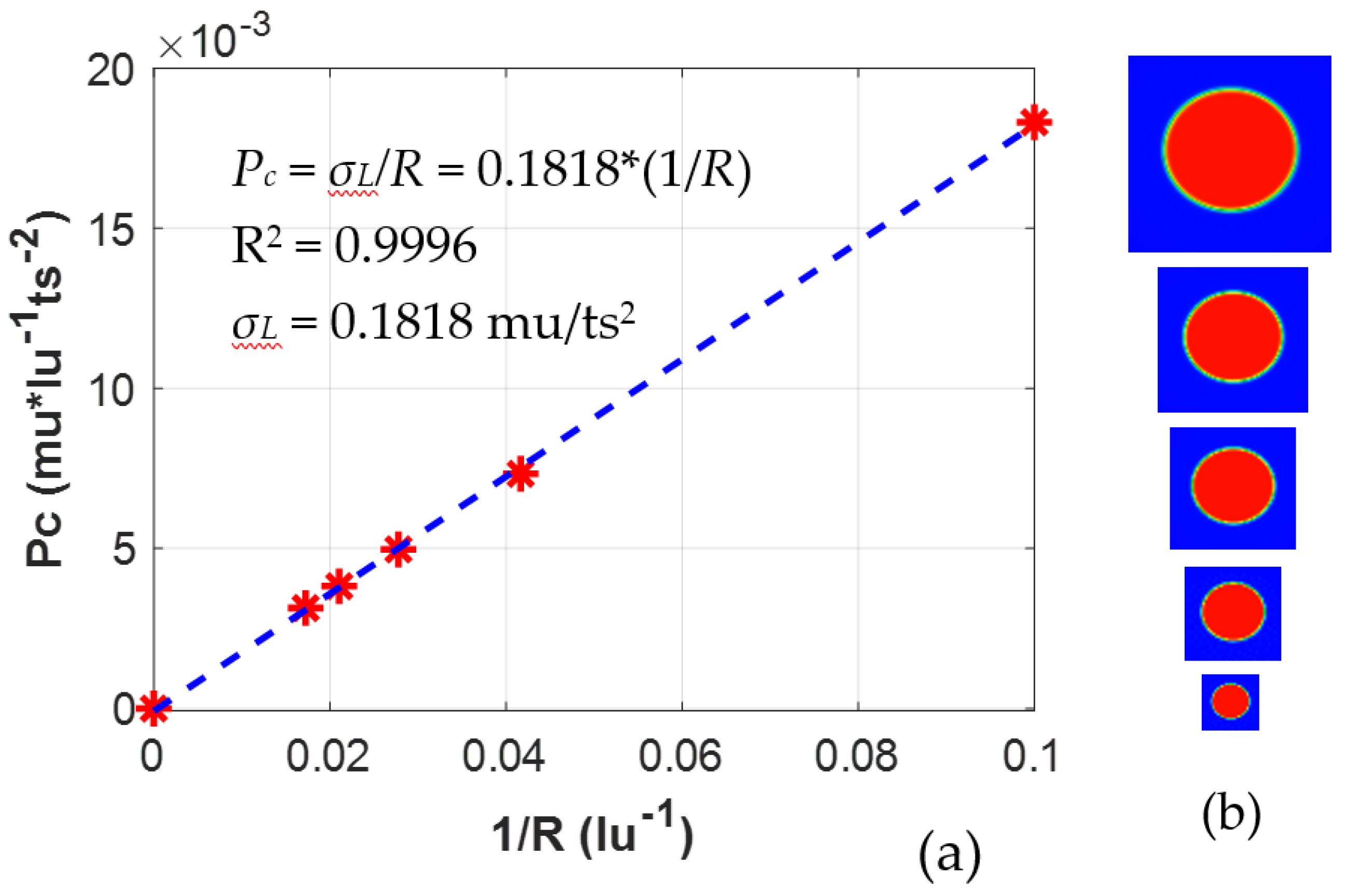
The flow regimes can be analyzed using Capillary number Ca and Reynold number Re:

$$Ca=\frac{\rho u\nu }{{\sigma }_L}$$

(20)

$$\mathrm{Re}=\frac{u{d}_{eff}(S)}{\nu }$$

(21)

where σ_L is the surface tension of liquid and d_eff is the effective hydraulic character length depending on the saturation history (S(t))—here, the geometric mean of the pore size distribution is adopted in this 2D simulation. For simplification and less computational expenses, gravity is neglected in this simulation. Hence, the Bond number is not involved in the analysis of capillary and viscous fingers.

(6)

Last but not least, due to the newly proposed P_c-S-a_nw and S-a_nw relationships [17], the specific interfacial area a_nw between the non-wetting and wetting fluid phase is defined using:

$$a_{nw}=\frac{{\displaystyle \sum _{i=1}^{N_{nw}}{A}_{i,nw}}}{{\displaystyle \sum _{i=1}^{N_T}{A}_i}}$$

(22)

and the detection of the wetting–non-wetting interface (A_i,nw) is achieved using the isosurface function in MATLAB [69].

3. Simulation Setup

3.1. Simulation Parameters for Fluid Properties

Solving SC-LBM is very computationally expensive work. In order to accelerate the simulation process, a few assumptions regarding the fluid properties are adopted as SC-LBM has been demonstrated to replicate physical experiments [52,57,62]. The parameters for controlling the properties of the two-phase fluids and simulation time are summarized in

Table 1. Settings of parameters for simulating two-phase immiscible fluids.

Parameters	Values
Initial ρw, ρn	2.0 mu/lu3
νw,vn	0.16 lu2/ts
Density variation	2.15 ± 0.08 mu/lu3
Δx	1.0 lu
Δt	1.0 ts
Gr	1.0
Gs,w, Gs,n	−0.5, 0.5
Total time steps Tf	5.0 × 105 ts

.

Here, the density ratio, kinematic viscosity ratio, lattice unit length, and lattice time step are set to one, so the basic lattice speed c = 1. The selection of G_r and ρ_j needs special care because there is a conflict between purifying the main component in each fluid phase and alleviating compressibility caused by fluid-fluid repulsive forces. By following the rules recommended by Martys and Douglas [47] and Huang, Thorne, Jr, Schaap, and Sukop [54], where 1.6 < G_rρ_j < 2.0 and ρ_j is the mixing density of two components, we are able to achieve a balance between those two effects. Based on parameter values in Table 1, the contact angle is set to zero according to:

$$\cos \theta =\frac{G_s^n-G_s^w}{G_r\frac{{\rho }_{\sigma }-{\rho }_{{\sigma }^{\prime }}}{2}}$$

(23)

where σ and σ′ are individually the main component and dissolved component in one fluid phase, respectively, and θ is the contact angle. Therefore, the surface tension of the wetting phase fluid can be given by the Young–Laplace equation with zero contact angle:

$$P_c=P_{in}-P_{out}=\frac{{\sigma }_L}{R}$$

(24)

where P_in and P_out are, respectively, the pressure of the components inside and outside of an SC-LBM single bubble simulation. Through simulating bubbles of various sizes (20~60 lu), the σ_L can be given by linear regression between P_c and 1/R, shown in Figure 2. The slope of the linear fitting function is σ_L.

With an aim to only qualitatively investigate the dynamic response of previously mentioned variables in 2D lattice space but not to replicate any physical experiment in the actual physical dimension, the unit transfer between the lattice and the physical domain is omitted and data are presented on the lattice unit.

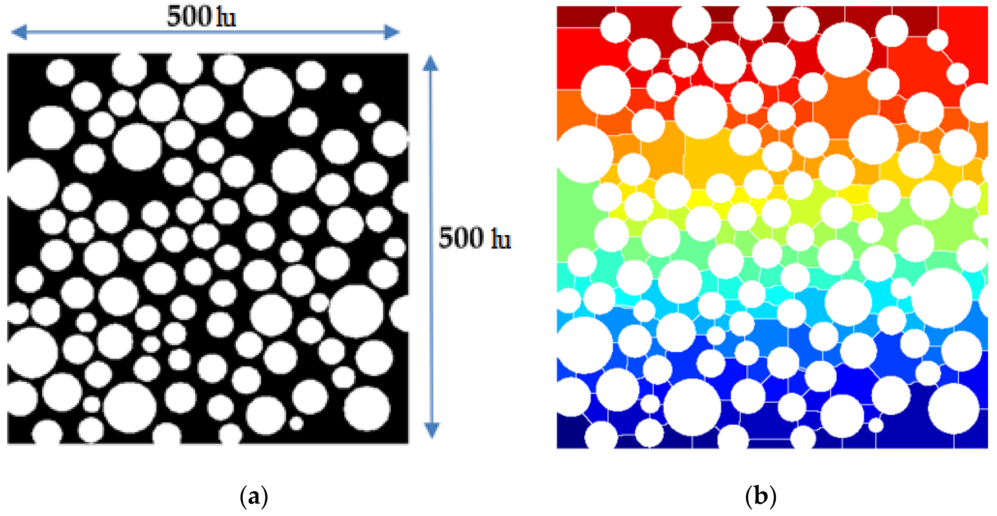
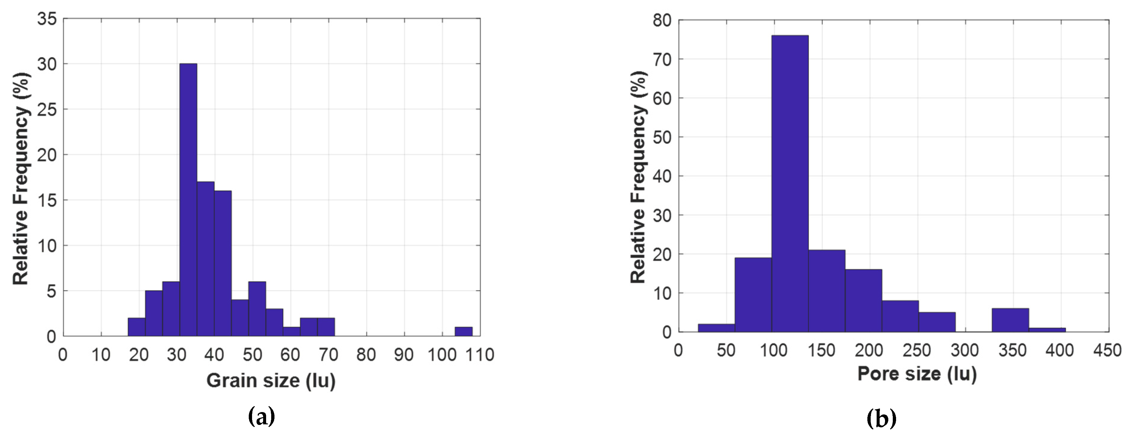
3.2. Two-Dimensional Porous Media and Hydraulic Boundary Conditions

To simulate the two-phase flow in a REV of porous media, a package of the perfect round particles is filled and fixed into a 500 × 500 × 1 lu³ quasi-two-dimensional (quasi-2D) domain with several particles intercepted by the boundaries of the quasi-2D domain in Figure 3a.

The black background is the pore space, where the two fluids seep through. The white circular disks represent the granular sand particles in this domain. This setup is designed to replicate the two-phase displacement, so the boundary conditions on both left and right are set to solid as same as each solid particle by applying the bounce-back scheme in Sukop and Thorne [68]:

$$f_i=f_{-i}$$

(25)

where −i represents the fluid molecules probability function symmetrically swapped, after an occurrence of the collision between fluids and the solid boundary. The boundary conditions for the top and bottom can be directly controlled by the density differences without any buffer zone, which can also be transferred into pressure differences using SC-LBM EOS in Equation (13). The pressure variation along the top and bottom is altered from 0% to 80% of initial fluid pressure to immediately apply a large pressure increment on the boundary to generate the transient flow condition. The traditional pressure and flux boundary conditions proposed by Zou and He [72] sometimes failed. Based on our modeling experience, the density dramatically increased after few time steps, and large densities then caused very high particle interactive force, subsequently compressing each fluid phase. This process eventually led to a final numerical instability. Hence, instead of applying boundary conditions developed by Zou and He [72], fixing a density difference with instant velocities as a pressure difference between two sides of the simulating domain has been accepted in a few previous studies [52,57,60,63,64,69]. The fluid of the wetting or non-wetting phase was completely filled into the pore space to set up the initial condition for the primary drainage or imbibition simulation.

As the domain edges axing some particles in the package, the grain size distribution (GSD) and pore size distribution (PSD) were redetected using image analysis in MATLAB. As shown in Figure 3b, the pore space was identified and measured using the pore network analyzing algorithm developed by Rabbani, Jamshidi, and Salehi [71]. The redetect GSD and PSD are separately depicted in Figure 4a,b. As shown in Figure 4, it should be noted that the porous media applied here cannot represent any natural geo-material in practical cases. As the mean pore size is 3–4 times of mean grain size with a high porosity of 44 ± 1%, the selected 2D porous media is very permeable (K_sat = 3.44 ± 0.13 lu²), and therefore, transitional flow regimes between laminar and turbulence might be possible. The specification of quasi-2D porous media is listed in

Table 2. Properties of quasi-2D porous media.

Setup Settings	Value
Domain size (lx = ly)	500 lu
Grain number	95
Porosity (n)	44 ± 1%
Mean grain size	39 ± 12 lu
Mean pore size	140 ± 64 lu
Geometric mean pore size	135 lu
Ksat	3.44 ± 0.13 lu2

.

4. Result and Discussion

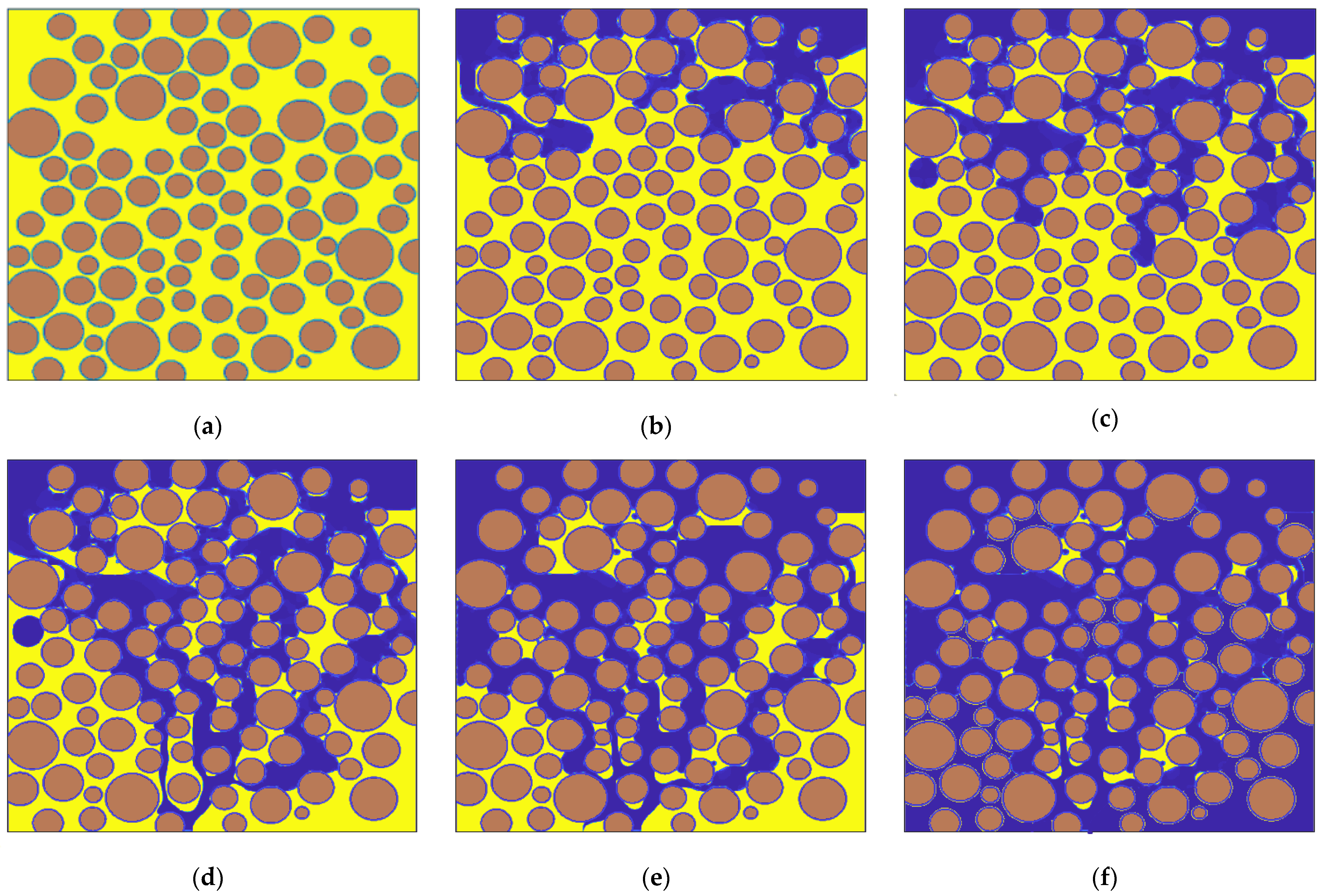
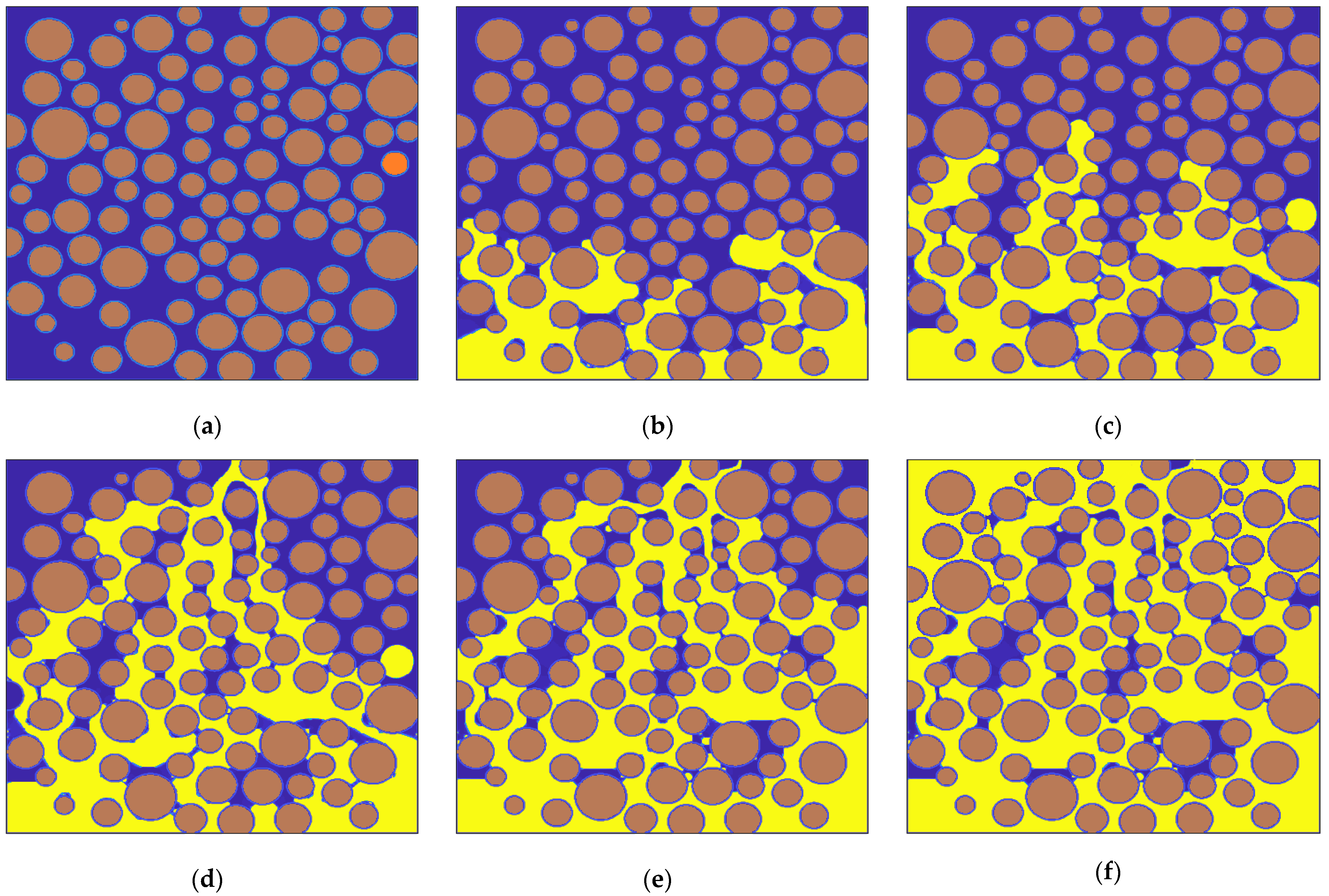
4.1. Demonstration of SC-LBM Simulation for One-Step In/Outflow

Figure 5 presents the one-step outflow simulation for the primary drainage test. From Figure 5a–f, each one illustrates the wetting phase distribution (highlighted in yellow) at six final equilibrium conditions, and corresponding non-wetting phase configurations are shade in blue as well. Originally, the porous media was fully saturated. With increasing the non-wetting phase density on top and decreasing the non-wetting phase density from the bottom in the same density boundary conditions. For this density boundary condition, mass conservation can be ensured with equal densities for both fluids, as the density input for the wetting phase is set to equal to the density output for the non-wetting phase. Additionally, by applying the LBM EOS (Equation (13)), this density pressure boundary can be directly seen as a pressure difference boundary. Since the non-wetting phase was injected from the top as shown in Figure 5a,b, the fluid-fluid interfaces advanced into the porous media. With the further increment of non-wetting phase pressure, in Figure 5c,d, a preferential flow path was produced and the non-wetting phase fluid break through the porous media down to the bottom of simulating domain. Comparing this numerical simulation and the standard pressure chamber SWRC test [73], there is no need to set up a low-permeable ceramic disk under the soil specimen. This ceramic disk ceases the air penetration through the pressure cell bottom in order to generate a sharp wetting front inside the specimen, which causes the difference between laboratory test and in-situ conditions. Therefore, such a preferential flow path can be physically replicated by SC-LBM. From Figure 5e,f, with additionally rising non-wetting phase pressure and decreasing wetting phase pressure, the wetting phase fluids located by two sides of the preferential path were finally expelled out of the porous media, and the residual wetting phase fluid was finally trapped inside the pore matrix. This series of figures demonstrate the capability of SC-LBM on replicating the multiphase physical phenomenon in regards to significant fluid-fluid separation (meniscus identification), non-wetting phase entry, fluid reconfiguration, preferential flow path, and residual fluid trapping, as the Shan–Chen pseudo-interactive forces (Equations (9) and (10)) fully reconstruct the immiscible multiphase interfaces.

Figure 6 shows the one-step inflow simulation for the primary imbibition test. Figure 6a–f shows the wetting phase fluid (highlighted in yellow) imbibed through porous media, and the corresponding non-wetting phase fluid distribution (shade in blue) at final equilibrium for six pressure boundary conditions are also given. Initially, the quasi-2D porous media was fully saturated by the non-wetting phase fluid. By increasing the wetting phase pressure/density at the bottom boundary and dropping the same pressure/density for the non-wetting phase on the top boundary, the wetting fluid suddenly imbibed into the domain bottom. Due to the finer pore matrix in simulating domain, a preferential flow path was generated again for the imbibition test. Finally, with further increasing wetting phase pressure, the porous media was completely flooded by wetting phase fluid, with only a few non-wetting phase bubbles trapped inside the pore matrix. The imbibition simulation reconfirms that the SC-LBM is a very powerful tool for predicting multiphase fluid hydrodynamics. Furthermore, an interesting finding is that the meniscus is highly dynamic according to the advancing velocity and direction as well. A concave meniscus for drainage test can be further stretched while for the imbibition test, under conditions of injecting wetting phase fluid, the concave meniscus can be alleviated or even reversed back to a convex meniscus advancing along the wetting front. This implies that under transient flow conditions, the dynamic meniscus might be dependent on the accelerating inertial effects in nonequilibrium transient flow imposed on meniscus [41,43] with dynamic contact angles [15,74,75] and pressure boundary conditions along the top and bottom of simulating domain. Hence, applying the Young–Laplace equation with a static contact angle as capillary forces in the Naiver–Stokes equation should not be able to replicate the multiphase dynamic behavior, because of the omission of meniscus dynamic or Helmholtz free energy [43,75] under transient flow conditions. Additionally, it is more suitable for the investigation of a steady-state multiphase flow in porous media, where capillary forces completely dominate the seepage.

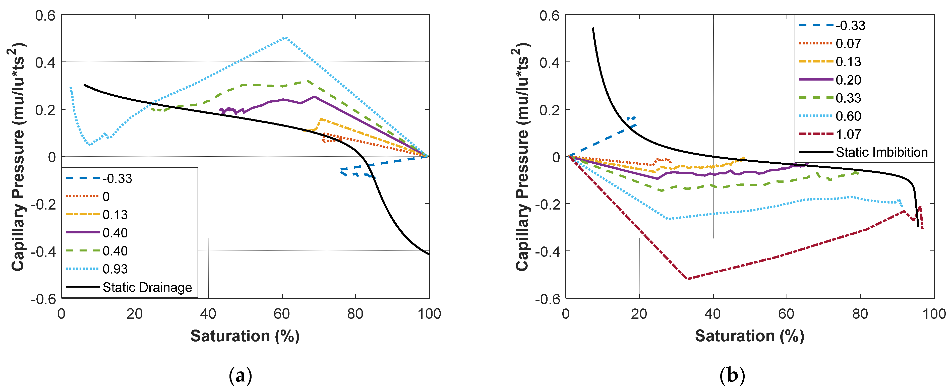
4.2. Comparison of Pc-S Curves between the Static and Transient Condition

Figure 7a–d separately illustrates the history of saturation and capillary pressure (P_c) for both drainage and imbibition. According to Figure 7a–d, after 3 × 10⁵ ts (lattice unit time/iteration steps), which is only 60% of the entire simulated time steps (5 × 10⁵ ts), all simulations finally achieve the equilibrium conditions, where there is no more wetting front advancing or flow. By suddenly applying different pressure boundary conditions since the second iteration step, a dynamic variation of P_c and S are observed from Figure 7a,b for primary drainage and Figure 7c,d for primary imbibition. Since the large pressure boundary applied on both the top for the non-wetting phase and the bottom for the wetting phase, both P_c and S manifest the sharp variation, and later approach to constant values for equilibrium. Such transient responses are the nonequilibrium P_c and S under transient flow conditions. However, as for the standard unsaturated soil test, all data points for each pair of suction and moisture have to be collected under static conditions. Because the conventional pressure cell requires an equilibrium condition to determine the soil suction by calculating the pressure difference between air and water. Whereas the tensiometer can be applied to detect the soil suction, the inevitable delay of the suction response still exists due to the permeability of the ceramic tip [76]. The SC-LBM allows an instantaneous determination of P_c and S, which provides a chance to study the dynamic behavior of P_c-S curves. The data points along the final equilibrium can be linked together as a static P_c-S curve fitted by Fredlund and Xing SWRC model [77], while the data points before the equilibrium are taken to draw the dynamic P_c-S curves for each pressure boundary condition, as shown in Figure 8.

However, a few disadvantages were also uncovered through the numerical investigation. As shown in Figure 7a, there is no exact final equilibrium for P_c under a pressure boundary of 0.93 mu/lu∙ts². This is due to the numerical issue that with such a larger density boundary applied, as in Figure 7b, the saturation is immediately decreased down to less than 10%. A numerical instability for the density might be potentially yielded. However, the specific reason for this is still in need of further investigation, and the numerical method requires improvement as well. Moreover, some negative pressure boundary conditions were adopted to achieve the full saturated and dry conditions. This is because the non-wetting phase entry value is dependent on the quasi-2D porous geometry [59], or in the practical expression of unsaturated soil mechanics: the pore size distribution determined from the initial soil density-dependent SWRC and grain size distribution [78]. In order to complete the full range of P_c-S curves, a few reversed boundary conditions have to be given to approaching the 100% saturation for drainage and 0% saturation for imbibition.

Figure 8a shows the overshooting dynamic P_c-S primary drainage curves in comparison to the static P_c-S curves marked in black solid fitting curves. For each S, the P_c under transient flow is larger than the static P_c under static conditions. A similar difference between static and dynamic P_c-S curves can also be found from Figure 8b, where for each S, the P_c for transient flow is higher than P_c for the static condition. This work is one of pioneering works in which the SC-LBM was applied to replicate the dynamic P_c-S curves, which was unveiled decades ago by physically experimental and theoretical studies such as Topp, Klute, and Peters [10], Hassanizadeh, Celia, and Dahle [15], etc. According to Figure 8a,b, it is clear that the larger the applied pressure boundary conditions, the further the dynamic P_c-S curves deviate from the static P_c-S curves. In the conventional test, we only take the data points from the no flow condition to plot the static P_c-S curves, and the fitting parameters dominate the constitutive behavior of unsaturated soil for Richards’ model [3]. Thus, the question was raised of how a static P_c-S relationship can be used to simulate the dynamic two-phase flow in unsaturated soil, while there is such a difference between dynamic and static P_c-S curves. To deeply investigate the potential reasons leading to such a difference, in the following content, the P_c-S dynamic behavior is analyzed with the interfacial area proposed by Hassanizadeh and Gray [17], and flow regimes quantified by hydrodynamic dimensionless numbers including Capillary and Reynolds numbers (Ca and Re).

Nevertheless, despite the finding of dynamic P_c-S using SC-LBM, some drawbacks are reconfirmed. Except for the problems about reversing boundary conditions and large pressure boundary conditions mentioned previously, the non-wetting phase entry values for each dynamic curve are not clearly defined in Figure 8a,b. This is due to setting the lower temporal resolution for such a fast transient flow test. Only one frame was recorded when a large pressure boundary condition was applied. However, the dynamic curves still quantitatively manifest the responses of P_c and S under transient flow.

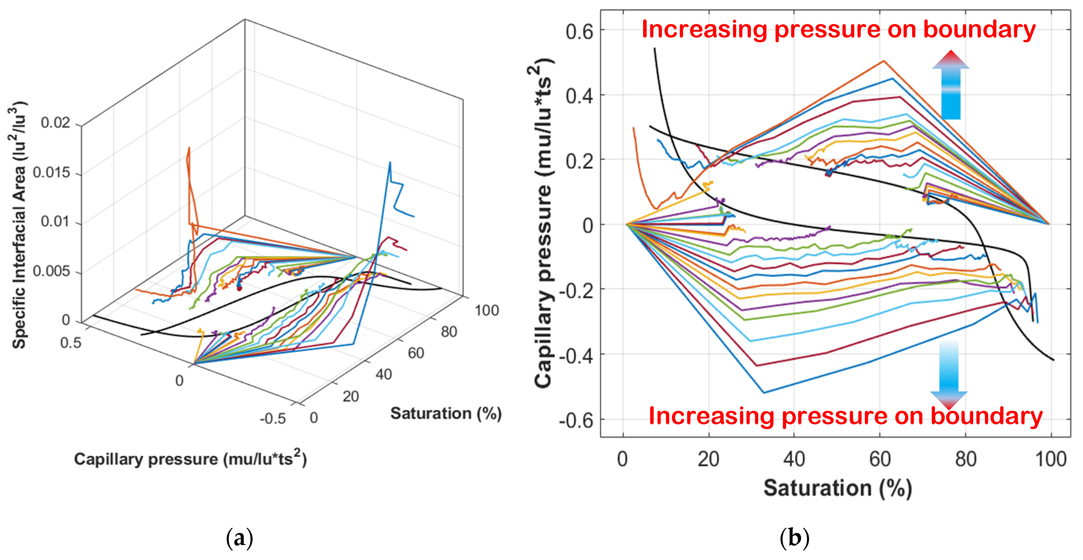
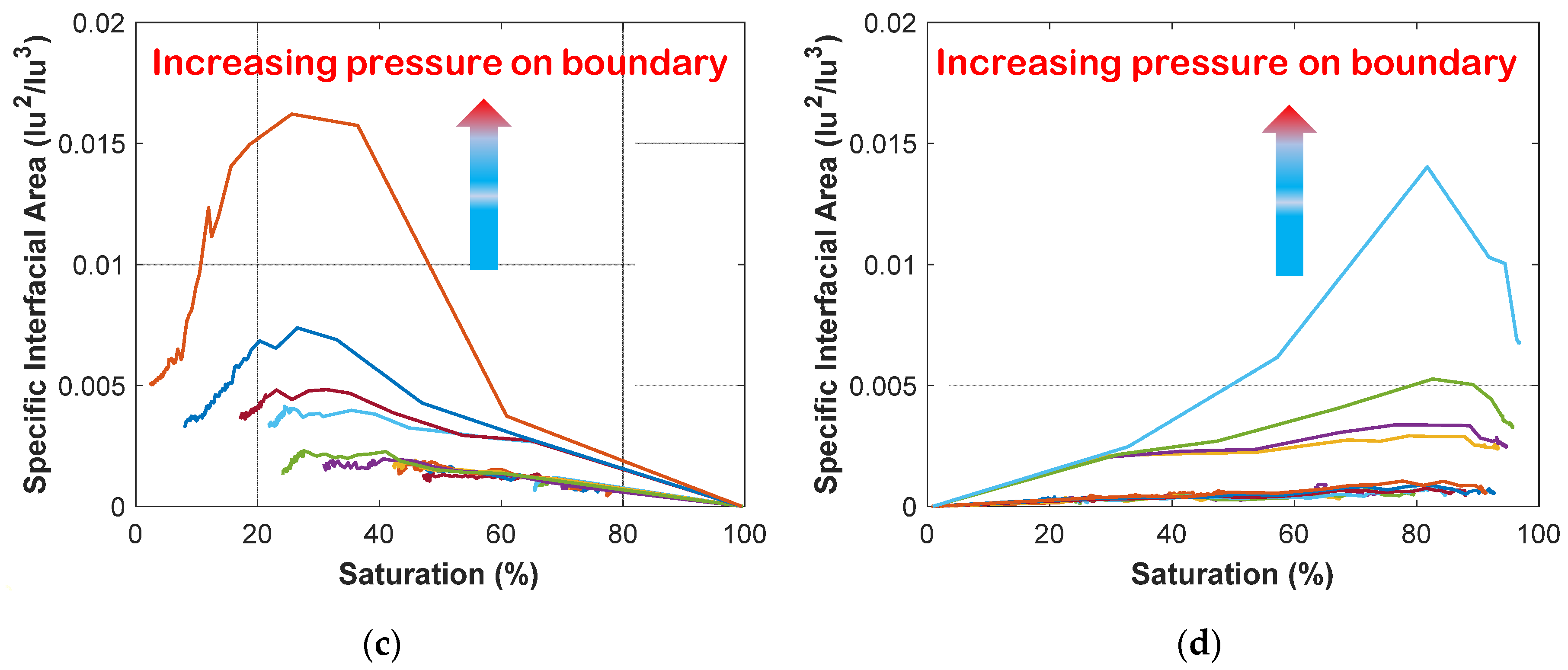
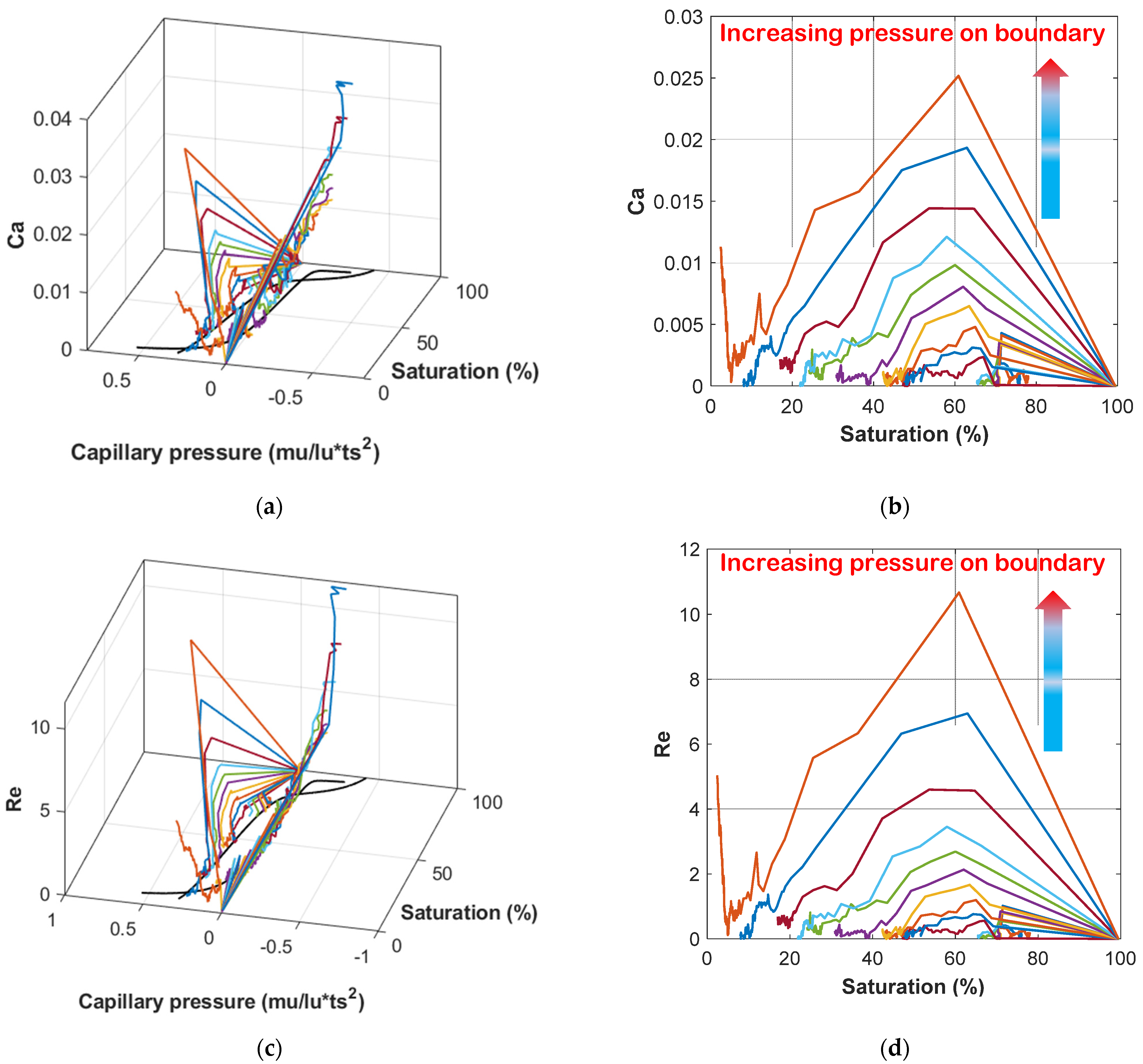
4.3. Pc, S, a_nw Dynamics, and Flow Regimes for Non-Equilibrium Condition

Figure 9b shows the P_c-S-a_nw relationship in the three-dimensional (3D) plot. The project of these relationships is individually plotted into a 2D space of S-a_nw for drainage in Figure 9a and imbibition in Figure 9c. Hassanizadeh and Gray [17] proposed a unique constitutive relationship among three state variables in terms of P_c, S, and a_nw. The uniqueness of such a 3D constitutive surface has been confirmed in previous pore-network models, and SC-LBM studies for equilibrium conditions [52,79]. Porter, Schaap, and Wildenschild [52] successfully fitted a parabolic surface into the P_c-S curves in terms of drainage, imbibition, and hysteresis scanning curves generated using the SC-LBM model. However, the question of whether such a 3D parabolic surface is still unique for transient flow conditions has been rarely studied using SC-LBM. According to Figure 9a, it is apparent that it is not possible to fit a parabolic surface into this series of P_c-S curves; it is only possible to fit one surface between each pair of drainage and imbibition curves. Therefore, the SC-LBM results in Figure 9 reconfirmed the non-uniqueness of P_c-S-a_nw constitutive surface under transient flow conditions, which was already found by previous physical micromodel studies [39] and pore network simulation [79,80]. Additionally, as shown in Figure 9c,d, the larger the pressure boundary applied for either drainage and imbibition, the larger a_nw can be generated. For drainage, this enlarged a_nw demonstrates the extension of the meniscus during a fast transient flow as the brown, blue and red curves of S-a_nw depicted in Figure 9c. For imbibition, the fast flow conditions can not only reduce the interfacial area for smaller pressure boundary conditions but also reverse it from concave to convex under a large pressure boundary condition, so an extension of the reversed meniscus can be manifested as the blue and green S-a_nw curves in Figure 9d. Based on this finding, we are able to reconfirm the extension of an interfacial area for a fast two-phase seepage process [39,80].

Figure 10a presents the P_c-S-Ca relationship in a 3D plot, which shows that under low Ca, the P_c-S curves can be closer to the static one, and the dynamic P_c-S curves further deviated from the static one because of the higher pore velocity in Ca. Similar behavior can also be found from the 3D P_c-S-Re relationship in Figure 10c, because both Re and Ca are functions of the pore velocity (Equations (20) and (21)). Due to the unstable velocities for imbibition curves at final equilibrium, only the drainage S-Ca and S-Re curves are separately projected in the 2D S-Ca plane in Figure 10b and S-Re plane in Figure 10d for additional discussion. Here, the Re was introduced as an indicator to quantify the ratio between inertial and viscous effects. Because there are difficulties in the image analysis for consistently measuring the variation of the mean pore diameter for each phase fluid, to simplify the calculation of Re, a geometric mean pore diameter timed by historical saturation is, thus, selected. According to Figure 10b,d, with the pore velocity suddenly increased by applying a larger pressure boundary condition to the highly non-equilibrium transient flow condition and a later return to zero after re-equilibrium, both Ca and Re increase up to a peak value followed by a recession down to nearly zero. There are slight fluctuations of Ca and Re at the final stage, and they are caused by the numerical instability on the velocity field. Based on the definition of Ca, the further the dynamic S-Ca deviated from the static one, the higher the viscous effect predominates the flow regime rather than the capillary effect. Furthermore, when the Re is considered in the analysis, as given in Figure 10d, we can see that the larger the pore velocity, the higher the convective inertial effects predominate the flow regimes over the viscous effect. In a conventional flow regime analysis for two-phase flow seepage, Ca was usually taken into consideration without Re. This somehow leads to an overlook of the convective inertial effect, which in fact can be produced under suddenly applying large pressure boundary conditions. Therefore, based on our SC-LBM simulation, the capillary effect only dominates the transient flow if the Re is smaller than 1, while the dynamic P_c-S curves generated by fast-rising pressure boundary conditions manifest a transitional flow regime between 1 and 15 of Re. These findings also imply that under the laminar flow regime, the static P_c-S curves should be preserved for Richards’ model and the assumption of instantaneous equilibrium does not seem significantly violated. The dynamic P_c-S might be a manifestation of the convective inertial effect under a transitional flow regime. Thus, for one certain porous media, the dynamic effect in P_c-S under transient flow conditions should be fully dependent on the speed of variation and magnitude of pressure and flux boundary conditions. This type of boundary conditions may happen for extreme circumstances, such as intensive rainfall, fast surface water table rising during the flood, large pressure of gas and brine invading through oil/gas reservoir, and CO₂ sequestration. Furthermore, beyond the P_c-S, the K_r-S, as the other constitutive relationship in Richards’ model, should also be extrapolated for understanding the dynamic effects.

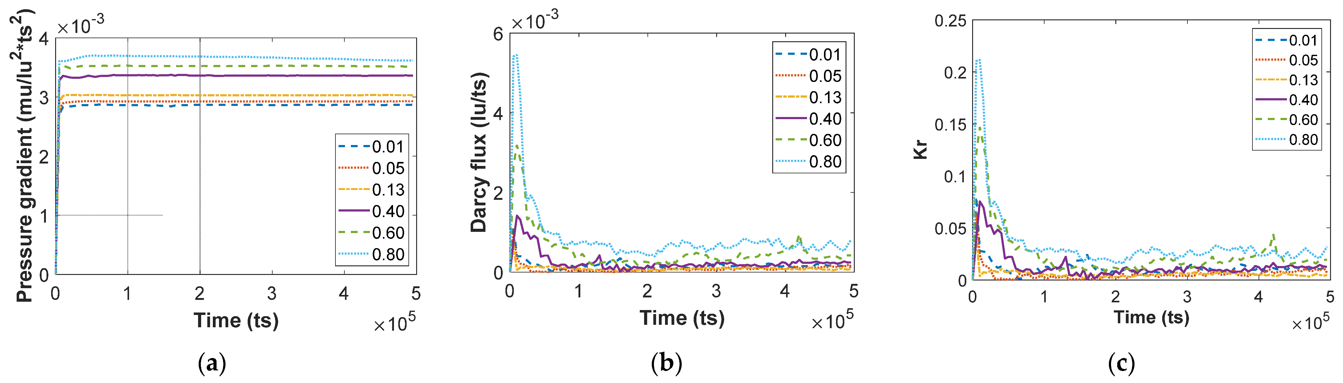
4.4. Discussion on Relative Permeability for Transient Multiphase Flow

Figure 11a,b shows the historical detection of wetting phase pressure gradient and Darcy flux q for drainage. Based on Equations (18) and (19), the relative permeability is calculated in Figure 11c. As can be observed in Figure 11a,b, for each constant pressure gradient, the seepage flux initiate from zero at one equilibrium stage, and climb to a peak flux followed by a dropping down to nearly zero to achieve another equilibrium when a transient flow ceases. Due to the non-monotonic relation between Darcy flux and wetting phase pressure gradient along the same time axis, for each boundary condition, the relative permeability also presents such a damping behavior. This is a direct observation of the dynamic behavior of the wetting phase from one state to another state. It should be governed by the full Navier–Stokes equation without the elimination of inertial (material derivative), including both accelerating and convective inertial. Once the boundary varied, there should be an accelerating and deaccelerating process between one and another equilibrium state. However, because of the assumption on instantaneous equilibrium, the steady-state seepage law-Darcy’s law, which was found under constant seepage flux by Darcy and Bazin [81], therefore, can be extended to two-phase Darcy’s law by introducing the concept of relative permeability. Whether the concept of relative permeability works for Richards’ model somehow also relies on a lower seepage flux, which can be yielded by a slow variation of pressure boundary conditions [82], and intrinsic hydraulic properties of porous media [12]. Then, under the assumption of instantaneous equilibrium, for each P_c or S, the K_r-S function can be predicted from P_c-S curves using permeability functions such as Brooks [83], Mualem [84], Fredlund et al. [85], etc. Under full transient flow conditions, the seepage flux for each phase should encounter a damping behavior, while relative permeability is a concept founded on steady-state conditions instantaneously achieved within a slow transient process.

Thus far, the velocity data from SC-LBM under large pressure boundary conditions still shows fluctuations and non-zero conditions at the final equilibrium stage, as shown in Figure 11b. The same fluctuated and non-zero Darcy flux at the ending stage can also be found in Figure 10b,d. Those abnormal behavior are because the fluid phase left in the pore matrix might have high spurious velocities around solid particles. The first layer of spurious velocities has been already filtered out on the first layer outside of each solid particle by the post-processing algorithm in MATLAB. However, there might still exist more than one layer of spurious velocities outside of solid particles. Whether to filter them out should be determined case by case depending on each simulation corresponding to each pressure boundary condition. These unstable velocities constrain the quantitative analysis, but still offer a great vision to discover transient flow qualitatively.

5. Conclusions

The two-dimensional multiphase, multicomponent Shan–Chen Lattice Boltzmann Method (SC-LBM) was implemented to simulate transient two-phase seepage through porous media. The transient flow conditions were generated by suddenly applying varies of the magnitude of pressure boundary conditions between the top for non-wetting phase fluid and the bottom for wetting phase fluid on the 2D porous package. The left- and right-hand sides of the domain were set as solid boundary conditions. This stimulating setup replicates the standard pressure cell experiment under an idealized condition where there is not a low permeable ceramic disk under the specimen. The animation of SC-LBM reconstructs the fluid phase entries, two-phase displacement, preferential flow path and phase trapping. Both the static and dynamic P_c-S curves under equilibrium and non-equilibrium can be manifested by this simulating data. The non-uniqueness of the P_c-S-a_nw relationship found from previous studies is reconfirmed as well. To investigate the impacts of flow regimes, the dynamic P_c-S curves are correlated with Ca and Re. Through the analysis of the predominant effects using those two dimensionless groups, it seems that the dynamic P_c-S curve is produced by small accelerating and convective inertial effects predominating in transitional flow regimes. As both Ca and Re are functions of pore velocity, the reason for higher pore velocity is due to the fast variation of larger pressure boundary conditions. In addition, the larger the pressure boundary applied immediately, the further the dynamic P_c-S curves deviate from the static P_c-S curves. Thus, the P_c-S relationships, originally determined by pressure cell test, somehow overlook the impacts of fast variation of pressure boundary conditions potentially existing in nature. Additionally, the K_r varying against time is also calculated to manifest the accelerating and later deaccelerating between the two equilibrium states. The validity of the instantaneous equilibrium assumption is, therefore, discussed based on the research findings. According to the data from these SC-LBM simulations, it seems that this assumption could be satisfied if the flow regime remains strictly under the laminar. The dynamic effects significantly appear if Re is above 1.

However, this numerical simulation still owns few limitations. First, it is only a quasi-2D simulation. The dependence of 2D simulation is inevitably overlooked in this study. In the future, the 3D SC-LBM should be carried out to validate the findings from this work. Second, the velocities determined from this model encounter a fluctuation. This is concerning to the improvement of SC-LBM by incorporating a multi-relaxation scheme and upgrading the fluid-solid/fluid-fluid interactive forces with the density and velocity correcting steps. Thus, this free-accessed open-source library-Mechsys can also be upgraded to continue this discovery in the future. Third, the unity ratio of density and viscosity can also be altered to achieve more physically experimental conditions. In principle, the numerical results provide a good manifestation of the dynamic effects of multiphase flow in quasi-2D porous media under idealized simulating conditions of SC-LBM. The SC-LBM is a very powerful tool for the investigation of dynamic multiphase flow in porous media. By further developing this numerical method, it is expected that the qualitative analysis can be upgraded to a better quantitative analysis for natural geomaterial with immiscible fluids.

References

1. Bear, J. Dynamics of Fluids in Porous Media; American Elsevier Publishing Company: New York, NY, USA, 1972. [Google Scholar]
2. Buckley, S.E.; Leverett, M. Mechanism of fluid displacement in sands. Trans. AIME 1942, 146, 107–116. [Google Scholar] [CrossRef]
3. Richards, L.A. Capillary conduction of liquids through porous mediums. J. Appl. Phys. 1931, 1, 318–333. [Google Scholar] [CrossRef]
4. Fredlund, D.G.; Rahardjo, H. Soil Mechanics for Unsaturated Soils; John Wiley & Sons: Hoboken, NJ, USA, 1993. [Google Scholar]
5. Lu, N.; Likos, W.J. Unsaturated Soil Mechanics; John Wiley & Sons: Hoboken, NJ, USA, 2004. [Google Scholar]
6. Khalili, N.; Khabbaz, M. A unique relationship of chi for the determination of the shear strength of unsaturated soils. Geotechnique 1998, 48, 681–687. [Google Scholar] [CrossRef]
7. Fredlund, D.G.; Morgenstern, N.R. Stress state variables for unsaturated soils. J. Geotech. Geoenviron. Eng. 1977, 103, 447–466. [Google Scholar]
8. Vanapalli, S.; Fredlund, D. Comparison of different procedures to predict unsaturated soil shear strength. Geotech. Spec. Publ. 2000, 195–209. [Google Scholar] [CrossRef] [Green Version]
9. Alonso, E.E.; Gens, A.; Josa, A. A constitutive model for partially saturated soils. Géotechnique 1990, 40, 405–430. [Google Scholar] [CrossRef] [Green Version]
10. Topp, G.; Klute, A.; Peters, D. Comparison of water content-pressure head data obtained by equilibrium, steady-state, and unsteady-state methods. Soil Sci. Soc. Am. J. 1967, 31, 312–314. [Google Scholar] [CrossRef]
11. Smiles, D.; Vachaud, G.; Vauclin, M. A test of the uniqueness of the soil moisture characteristic during transient, nonhysteretic flow of water in a rigid soil. Soil Sci. Soc. Am. J. 1971, 35, 534–539. [Google Scholar] [CrossRef]
12. Stauffer, F. Time dependence of the relations between capillary pressure, water content and conductivity during drainage of porous media. In Proceedings of the IAHR Symposium on Scale Effects in Porous Media, Thessaloniki, Greece, 28 August–1 September 1978; pp. 3–35. [Google Scholar]
13. Vachaud, G.; Vauclin, M.; Wakil, M. A study of the uniqueness of the soil moisture characteristic during desorption by vertical drainage. Soil Sci. Soc. Am. J. 1972, 36, 531–532. [Google Scholar] [CrossRef]
14. Wana-Etyem, C. Static and Dynamic Water Content-Pressure Head Relations of Porous Media. Ph.D. Thesis, Colorado State University, Fort Collins, CO, USA, 1982. [Google Scholar]
15. Hassanizadeh, S.M.; Celia, M.A.; Dahle, H.K. Dynamic effect in the capillary pressure–saturation relationship and its impacts on unsaturated flow. Vadose Zone J. 2002, 1, 38–57. [Google Scholar] [CrossRef]
16. Barenblatt, G.I.; Vinnichenko, A. Non-equilibrium seepage of immiscible fluids. Adv. Mech. 1980, 3, 35–50. [Google Scholar]
17. Hassanizadeh, S.M.; Gray, W.G. Toward an improved description of the physics of two-phase flow. Adv. Water Resour. 1993, 16, 53–67. [Google Scholar] [CrossRef]
18. Kalaydjian, F. A macroscopic description of multiphase flow in porous media involving spacetime evolution of fluid/fluid interface. Transp. Porous Media 1987, 2, 537–552. [Google Scholar] [CrossRef]
19. O’Carroll, D.M.; Phelan, T.J.; Abriola, L.M. Exploring dynamic effects in capillary pressure in multistep outflow experiments. Water Resour. Res. 2005, 41. [Google Scholar] [CrossRef] [Green Version]
20. Sakaki, T.; O’Carroll, D.M.; Illangasekare, T.H. Direct quantification of dynamic effects in capillary pressure for drainage–wetting cycles. Vadose Zone J. 2010, 9, 424–437. [Google Scholar] [CrossRef]
21. O’Carroll, D.M.; Mumford, K.G.; Abriola, L.M.; Gerhard, J.I. Influence of wettability variations on dynamic effects in capillary pressure. Water Resour. Res. 2010, 46. [Google Scholar] [CrossRef] [Green Version]
22. Das, D.B.; Mirzaei, M. Dynamic effects in capillary pressure relationships for two-phase flow in porous media: Experiments and numerical analyses. AIChE J. 2012, 58, 3891–3903. [Google Scholar] [CrossRef] [Green Version]
23. Abidoye, L.K.; Das, D.B. Scale dependent dynamic capillary pressure effect for two-phase flow in porous media. Adv. Water Resour. 2014, 74, 212–230. [Google Scholar] [CrossRef] [Green Version]
24. Hanspal, N.S.; Das, D.B. Dynamic effects on capillary pressure–Saturation relationships for two-phase porous flow: Implications of temperature. AIChE J. 2012, 58, 1951–1965. [Google Scholar] [CrossRef] [Green Version]
25. Mirzaei, M.; Das, D.B. Dynamic effects in capillary pressure–saturations relationships for two-phase flow in 3D porous media: Implications of micro-heterogeneities. Chem. Eng. Sci. 2007, 62, 1927–1947. [Google Scholar] [CrossRef] [Green Version]
26. Mirzaei, M.; Das, D.B. Experimental investigation of hysteretic dynamic effect in capillary pressure–saturation relationship for two-phase flow in porous media. AIChE J. 2013, 59, 3958–3974. [Google Scholar] [CrossRef] [Green Version]
27. Scheuermann, A.; Galindo-Torres, S.; Pedroso, D.; Williams, D.; Li, L. Dynamics of water movements with reversals in unsaturated soils. In Proceedings of the 6th International Conference on Unsaturated Soils, UNSAT 2014, Sydney, Australia, 2–4 July 2014; pp. 1053–1059. [Google Scholar]
28. Chen, L. Hysteresis and Dynamic Effects in the Relationship between Capillary Pressure, Saturation, and Air-Water Interfacial Area in Porous Media. Ph.D. Thesis, The University of Oklahoma, Norman, OK, USA, 2006. [Google Scholar]
29. Diamantopoulos, E.; Durner, W. Dynamic nonequilibrium of water flow in porous media: A review. Vadose Zone J. 2012, 11. [Google Scholar] [CrossRef]
30. Yan, G.; Scheuermann, A.; Schlaeger, S.; Bore, T.; Bhuyan, H. Application of Spatial Time Domain Reflectometry for investigating moisture content dynamics in unsaturated sand. In Proceedings of the 11th International Conference on Electromagnetic Wave Interaction with Water and Moist Substances, Florence, Italy, 23–27 May 2016; p. 117. [Google Scholar]
31. Yan, G.; Li, Z.; Bore, T.; Galindo-Torres, S.; Schlaeger, S.; Scheuermann, A.; Li, L. An Experimental Platform for Measuring Soil Water Characteristic Curve under Transient Flow Conditions. In Advances in Laboratory Testing and Modelling of Soils and Shales (ATMSS); Springer: Cham, Switzerland, 2017; pp. 231–238. [Google Scholar] [CrossRef]
32. Yan, G.; Bore, T.; Galindo-Torres, S.; Scheuermann, A.; Li, Z.; Li, L. Primary imbibition curve measurement using large soil column test. In Proceedings of the 19th International Conference on Soil Mechanics and Geotechnical Engineering, Seoul, Korea, 17–22 September 2017; pp. 1261–1264. [Google Scholar]
33. Yan, G.; Li, Z.; Bore, T.; Scheuermann, A.; Galindo-Torres, S.; Li, L. The measurement of primary drainage curve using hanging column and large soil column test. In Proceedings of the GeoOttawa 2017, Ottawa, ON, Canada, 1–4 October 2017. [Google Scholar]
34. Yan, G.; Bore, T.; Galindo-Torres, S.; Scheuermann, A.; Li, L.; Schlaeger, S. An investigation of soil water retention behavior using large soil column test and multiphase Lattice Boltzmann simulation. In Proceedings of the 7th International Conference on Unsaturated Soils (UNSAT2018), Hong Kong, China, 3–5 August 2018. [Google Scholar]
35. Yan, G.; Bore, T.; Li, Z.; Schlaeger, S.; Scheuermann, A.; Li, L. Application of Spatial Time Domain Reflectometry for Investigating Moisture Content Dynamics in Unsaturated Loamy Sand for Gravitational Drainage. Appl. Sci. 2021, 11, 2994. [Google Scholar] [CrossRef]
36. Karadimitriou, N.; Joekar-Niasar, V.; Hassanizadeh, S.; Kleingeld, P.; Pyrak-Nolte, L. A novel deep reactive ion etched (DRIE) glass micro-model for two-phase flow experiments. Lab Chip 2012, 12, 3413–3418. [Google Scholar] [CrossRef] [Green Version]
37. Karadimitriou, N.; Hassanizadeh, S. A review of micromodels and their use in two-phase flow studies. Vadose Zone J. 2012, 11. [Google Scholar] [CrossRef]
38. Karadimitriou, N.; Musterd, M.; Kleingeld, P.; Kreutzer, M.; Hassanizadeh, S.; Joekar-Niasar, V. On the fabrication of PDMS micromodels by rapid prototyping, and their use in two-phase flow studies. Water Resour. Res. 2013, 49, 2056–2067. [Google Scholar] [CrossRef] [Green Version]
39. Karadimitriou, N.; Hassanizadeh, S.; Joekar-Niasar, V.; Kleingeld, P. Micromodel study of two-phase flow under transient conditions: Quantifying effects of specific interfacial area. Water Resour. Res. 2014, 50, 8125–8140. [Google Scholar] [CrossRef] [Green Version]
40. Ferrari, A.; Jimenez-Martinez, J.; Borgne, T.L.; Méheust, Y.; Lunati, I. Challenges in modeling unstable two-phase flow experiments in porous micromodels. Water Resour. Res. 2015, 51, 1381–1400. [Google Scholar] [CrossRef] [Green Version]
41. Ferrari, A.; Lunati, I. Direct numerical simulations of interface dynamics to link capillary pressure and total surface energy. Adv. Water Resour. 2013, 57, 19–31. [Google Scholar] [CrossRef]
42. Ferrari, A. Pore-Scale Modeling of Two-Phase Flow Instabilities in Porous Media. Ph.D. Thesis, University of Turin, Turin, Italy, 2014. [Google Scholar]
43. Ferrari, A.; Lunati, I. Inertial effects during irreversible meniscus reconfiguration in angular pores. Adv. Water Resour. 2014, 74, 1–13. [Google Scholar] [CrossRef]
44. Helland, J.O.; Friis, H.A.; Jettestuen, E.; Skjæveland, S.M. Footprints of spontaneous fluid redistribution on capillary pressure in porous rock. Geophys. Res. Lett. 2017, 44, 4933–4943. [Google Scholar] [CrossRef] [Green Version]
45. Shan, X.; Chen, H. Lattice Boltzmann model for simulating flows with multiple phases and components. Phys. Rev. E 1993, 47, 1815. [Google Scholar] [CrossRef] [Green Version]
46. Fan, L.; Fang, H.; Lin, Z. Simulation of contact line dynamics in a two-dimensional capillary tube by the lattice Boltzmann model. Phys. Rev. E 2001, 63, 051603. [Google Scholar] [CrossRef]
47. Martys, N.S.; Douglas, J.F. Critical properties and phase separation in lattice Boltzmann fluid mixtures. Phys. Rev. E 2001, 63, 031205. [Google Scholar] [CrossRef] [Green Version]
48. Tölke, J. Lattice Boltzmann simulations of binary fluid flow through porous media. Philos. Trans. R. Soc. Lond. A Math. Phys. Eng. Sci. 2002, 360, 535–545. [Google Scholar] [CrossRef]
49. Raiskinmäki, P.; Shakib-Manesh, A.; Jäsberg, A.; Koponen, A.; Merikoski, J.; Timonen, J. Lattice-Boltzmann simulation of capillary rise dynamics. J. Stat. Phys. 2002, 107, 143–158. [Google Scholar] [CrossRef]
50. Pan, C.; Hilpert, M.; Miller, C. Lattice-Boltzmann simulation of two-phase flow in porous media. Water Resour. Res. 2004, 40. [Google Scholar] [CrossRef]
51. Sukop, M. , Thorne, D.T., Jr. Lattice Boltzmann Modeling; Springer: Berlin/Heidelberg, Germany, 2006. [Google Scholar]
52. Porter, M.L.; Schaap, M.G.; Wildenschild, D. Lattice-Boltzmann simulations of the capillary pressure–saturation–interfacial area relationship for porous media. Adv. Water Resour. 2009, 32, 1632–1640. [Google Scholar] [CrossRef]
53. Gray, W.G.; Hassanizadeh, S.M. Paradoxes and realities in unsaturated flow theory. Water Resour. Res. 1991, 27, 1847–1854. [Google Scholar] [CrossRef]
54. Huang, H.; Thorne Jr, D.T.; Schaap, M.G.; Sukop, M.C. Proposed approximation for contact angles in Shan-and-Chen-type multicomponent multiphase lattice Boltzmann models. Phys. Rev. E 2007, 76, 066701. [Google Scholar] [CrossRef] [PubMed] [Green Version]
55. Sukop, M.C.; Or, D. Lattice Boltzmann method for modeling liquid-vapor interface configurations in porous media. Water Resour. Res. 2004, 40. [Google Scholar] [CrossRef]
56. Vogel, H.-J.; Tölke, J.; Schulz, V.; Krafczyk, M.; Roth, K. Comparison of a lattice-Boltzmann model, a full-morphology model, and a pore network model for determining capillary pressure–saturation relationships. Vadose Zone J. 2005, 4, 380–388. [Google Scholar] [CrossRef]
57. Schaap, M.G.; Porter, M.L.; Christensen, B.S.; Wildenschild, D. Comparison of pressure-saturation characteristics derived from computed tomography and lattice Boltzmann simulations. Water Resour. Res. 2007, 43. [Google Scholar] [CrossRef] [Green Version]
58. Li, Z.; Galindo-Torres, S.; Yan, G.; Scheuermann, A.; Li, L. Pore-scale simulations of simultaneous steady-state two-phase flow dynamics using a lattice Boltzmann model: Interfacial area, capillary pressure and relative permeability. Transp. Porous Media 2019, 129, 295–320. [Google Scholar] [CrossRef]
59. Li, Z.; Galindo-Torres, S.; Yan, G.; Scheuermann, A.; Li, L. A lattice Boltzmann investigation of steady-state fluid distribution, capillary pressure and relative permeability of a porous medium: Effects of fluid and geometrical properties. Adv. Water Resour. 2018, 116, 153–166. [Google Scholar] [CrossRef]
60. Galindo-Torres, S.; Scheuermann, A.; Li, L. Boundary effects on the Soil Water Characteristic Curves obtained from lattice Boltzmann simulations. Comput. Geotech. 2016, 71, 136–146. [Google Scholar] [CrossRef]
61. Ahrenholz, B.; Tölke, J.; Lehmann, P.; Peters, A.; Kaestner, A.; Krafczyk, M.; Durner, W. Prediction of capillary hysteresis in a porous material using lattice-Boltzmann methods and comparison to experimental data and a morphological pore network model. Adv. Water Resour. 2008, 31, 1151–1173. [Google Scholar] [CrossRef]
62. Landry, C.; Karpyn, Z.; Ayala, O. Relative permeability of homogenous-wet and mixed-wet porous media as determined by pore-scale lattice Boltzmann modeling. Water Resour. Res. 2014, 50, 3672–3689. [Google Scholar] [CrossRef] [Green Version]
63. Porter, M.L.; Schaap, M.G.; Wildenschild, D. Capillary pressure–saturation curves: Towards simulating dynamic effects with the Lattice-Boltzmann method. In Proceedings of the XVI International Conference on Computational Methods in Water Resources (CMWR), Copenhagen, Denmark, 19–22 June 2006. [Google Scholar]
64. Galindo-Torres, S.; Scheuermann, A.; Li, L.; Pedroso, D.; Williams, D. A Lattice Boltzmann model for studying transient effects during imbibition–drainage cycles in unsaturated soils. Comput. Phys. Commun. 2013, 184, 1086–1093. [Google Scholar] [CrossRef]
65. Yan, G.; Li, Z.; Bore, T.; Galindo-Torres, S.; Scheuermann, A.; Li, L. Dynamic Effect in Capillary Pressure–Saturation relationship using Lattice Boltzmann Simulation. In Proceedings of the 2nd International Symposium on Asia Urban GeoEngineering, Changsha, China, 24–27 November 2017. [Google Scholar]
66. Tang, M.; Zhan, H.; Ma, H.; Lu, S. Upscaling of dynamic capillary pressure of two-phase flow in sandstone. Water Resour. Res. 2019, 55, 426–443. [Google Scholar] [CrossRef] [Green Version]
67. Cao, Y.; Tang, M.; Zhang, Q.; Tang, J.; Lu, S. Dynamic capillary pressure analysis of tight sandstone based on digital rock model. Capillarity 2020, 3, 28–35. [Google Scholar] [CrossRef]
68. Sukop, M.C.; Thorne, D.T., Jr. Lattice Boltzmann Modeling—An Introduction for Geoscientists and Engineers; Springer: Berlin/Heidelberg, Germany, 2007. [Google Scholar]
69. Galindo-Torres, S.; Scheuermann, A.; Pedroso, D.; Li, L. Effect of boundary conditions on measured water retention behavior within soils. In Proceedings of the AGU Fall Meeting Abstracts, San Francisco, CA, USA, 9–13 December 2013; p. 1516. [Google Scholar]
70. Pooley, C.; Furtado, K. Eliminating spurious velocities in the free-energy lattice Boltzmann method. Phys. Rev. E 2008, 77, 046702. [Google Scholar] [CrossRef] [Green Version]
71. Rabbani, A.; Jamshidi, S.; Salehi, S. An automated simple algorithm for realistic pore network extraction from micro-tomography Images. J. Pet. Sci. Eng. 2014, 123, 164–171. [Google Scholar] [CrossRef]
72. Zou, Q.; He, X. On pressure and velocity boundary conditions for the lattice Boltzmann BGK model. Phys. Fluids 1997, 9, 1591–1598. [Google Scholar] [CrossRef] [Green Version]
73. ASTM D6836-02. Test Methods for Determination of the Soil Water Characteristic Curve for Desorption Using a Hanging Column, Pressure Extractor, Chilled Mirror Hygrometer, and/or Centrifuge; American Society for Testing and Materials (ASTM) International: West Conshohocken, PA, USA, 2008. [Google Scholar]
74. Sheng, P.; Zhou, M. Immiscible-fluid displacement: Contact-line dynamics and the velocity-dependent capillary pressure. Phys. Rev. A 1992, 45, 5694. [Google Scholar] [CrossRef] [Green Version]
75. Hassanizadeh, S.M.; Gray, W.G. Thermodynamic basis of capillary pressure in porous media. Water Resour. Res. 1993, 29, 3389–3405. [Google Scholar] [CrossRef] [Green Version]
76. Klute, A.; Gardner, W. Tensiometer Response Time. Soil Sci. 1962, 93, 204–207. [Google Scholar] [CrossRef]
77. Fredlund, D.G.; Xing, A. Equations for the soil-water characteristic curve. Can. Geotech. J. 1994, 31, 521–532. [Google Scholar] [CrossRef]
78. Zhou, A.-N.; Sheng, D.; Carter, J. Modelling the effect of initial density on soil-water characteristic curves. Geotechnique 2012, 62, 669–680. [Google Scholar] [CrossRef] [Green Version]
79. Joekar-Niasar, V.; Hassanizadeh, S.M. Uniqueness of specific interfacial area–capillary pressure–saturation relationship under non-equilibrium conditions in two-phase porous media flow. Transp. Porous Media 2012, 94, 465–486. [Google Scholar] [CrossRef] [Green Version]
80. Joekar Niasar, V.; Hassanizadeh, S.; Dahle, H. Non-equilibrium effects in capillarity and interfacial area in two-phase flow: Dynamic pore-network modelling. J. Fluid Mech. 2010, 655, 38–71. [Google Scholar] [CrossRef]
81. Darcy, H.; Bazin, H. Recherches Hydrauliques: Recherches Expérimentales Sur L’éCoulement de L’Eau Dans Les Canaux Découverts. 1Ère Partie; Dunod: Paris, France, 1865; Volume 1. [Google Scholar]
82. ASTM D7664-10. Standard Test Methods for Measurement of Hydraulic Conductivity of Unsaturated Soils; American Society for Testing and Materials (ASTM) International: West Conshohocken, PA, USA, 2010. [Google Scholar]
83. Brooks, R.H. Hydraulic Properties of Porous Media; Colorado State University: Fort Collins, CO, USA, 1964. [Google Scholar]
84. Mualem, Y. A new model for predicting the hydraulic conductivity of unsaturated porous media. Water Resour. Res. 1976, 12, 513–522. [Google Scholar] [CrossRef] [Green Version]
85. Fredlund, D.; Xing, A.; Huang, S. Predicting the permeability function for unsaturated soils using the soil-water characteristic curve. Can. Geotech. J. 1994, 31, 533–546. [Google Scholar] [CrossRef]
Figure 1. D2Q9 scheme illustrates the nine discrete velocities (ei, i = 0~8) for a probability function (fi) at a single local node in the entire simulating domain.
Energies 14 04044 g001
Figure 2. Lattice surface tension (σL) determination: (a) The linear regression into data points between Pc and 1/R for determining σL using the Young–Laplace law for θ = 0; (b) The bubbles simulation in five different sizes varying from the diameter of 20 to 60 lu for the determination of σL.
Energies 14 04044 g002
Figure 3. The simulation domain and setup of quasi-two-dimensional (quasi-2D) porous media: (a) Simulation setup and solid particles package; (b) The measurement of the grain size distribution (GSD) and pore size distribution (PSD), using an image analysis algorithm developed by Rabbani et al. [71].
Energies 14 04044 g003
Figure 4. The quasi-2D porous media: (a) The histogram of grain size; (b) The histogram of pore size.
Energies 14 04044 g004
Figure 5. The demonstration of one-step outflow simulation using SC-LBM: (af) showing the non-wetting phase fluid (highlighted in blue) invading into the porous media (highlighted in brown) and the wetting phase fluid (highlighted in yellow) pushed out of porous media for six different pressure differences between the top and the bottom boundaries (0–1.07 mu/lu∙ts2).
Energies 14 04044 g005
Figure 6. The demonstration of one-step inflow simulation using SC-LBM: (af) showing the non-wetting phase fluid (highlighted in yellow) imbibed into the porous media (highlighted in brown) and the wetting phase fluid (highlighted in blue) pushed out of porous media for six different pressure differences between the top and the bottom boundaries (0–1.07 mu/lu∙ts2).
Energies 14 04044 g006
Figure 7. The historical detection of capillary pressure (Pc) and saturation (S). The legend shows the pressure boundary conditions with a lattice pressure unit of mu/lu∙ts2: (a,b) The primary drainage (one-step outflow simulation); (c,d) The primary imbibition (one-step inflow simulation).
Energies 14 04044 g007
Figure 8. The dynamic capillary pressure–saturation (Pc-S) curves under transient flow conditions versus the static Pc-S curves fitted in the model by Fredlund and Xing [77] (the legend is pressure boundary conditions in the unit of mu/lu∙ts2): (a) The dynamic drainage curve; (b) The dynamic imbibition curve.
Energies 14 04044 g008
Figure 9. The Pc-S-anw relationships under transient flow conditions (pressure boundaries labeled): (a) Pc-S-anw in 3D plot; (b) Projection of the Pc-S-anw relationships on the Pc-S plane; (c) Projection of the Pc-S-anw relationships on the S-anw plane; (d) Projection of the Pc-S-anw relationships on the S-anw plane.
Energies 14 04044 g009aEnergies 14 04044 g009b
Figure 10. The dynamic Pc-S with flow regimes in terms of Re and Ca (pressure boundaries labeled): (a) Pc-S-Ca in 3D plot; (b) Projection of 3D Pc-S-Ca into S-Ca plane for drainage; (c) Pc-S-Re in 3D plot; (d) Projection of 3D Pc-S-Re into S-Re plane for drainage.
Energies 14 04044 g010
Figure 11. The estimation of the dynamic relative permeability for drainage: (a) Wetting phase pressure gradient variation; (b) Wetting phase Darcy flux variation; (c) The trial on the calculation of the relative permeability changing with time. The legend lists different pressure boundary conditions applied on the simulating domain.
Energies 14 04044 g011