Fault Detection and Diagnosis Method of Distributed Photovoltaic Array Based on Fine-Tuning Naive Bayesian Model

Abstract

With the widespread attention and research of distributed photovoltaic (PV) systems, the fault detection and diagnosis problems of distributed PV systems has become increasingly prominent. To this end, a distributed PV array fault diagnosis method based on fine-tuning Naive Bayes model for the fault conditions of PV array such as open-circuit, short-circuit, shading, abnormal degradation, and abnormal bypass diode is proposed. First, in view of the problem of less distributed PV fault data, a fine-tuning Naive Bayes model (FTNB) is proposed to improve the diagnosis accuracy. Second, the failure sample set is used to train the model. Then, the maximum power point data of the PV inverter and the meteorological data are collected for fault diagnosis. Finally, the effectiveness and accuracy of the proposed method are verified by the analysis of simulation. In addition, this method requires only a small number of fault sample sets and no additional measurement equipment is required, which is suitable for real-time monitoring of distributed PV systems.

1. Introduction

In recent years, environmental pollution and climate change have become increasingly serious. PV systems have received more and more attention because of their advantages of cleanliness, high efficiency, and ease of installation [1]. In recent years, the PV power generation system has developed fast in China. According to statistics from the National Energy Commission, China became the world’s largest country in PV installations in 2015. As of the end of February 2020, distributed PV power generation systems had added 12.2 million kilowatts, an increase of 41.3% year-on-year [2].

In terms of reducing the cost of PV power generation, in addition to efforts to improve conversion efficiency and reduce the cost of solar cells, effective operation and maintenance of PV systems is also very important [3]. PV array is the most important component of the PV system, which is usually operated in an outdoor exposed condition and is prone to various failures [4]. This will inevitably reduce the output power of the PV system, greatly reduce the efficiency of the PV system, and even cause a fire. However, the conventional manual inspection, operation, and maintenance of PV arrays are very time-consuming, and due to the uneven level of skills of operation and maintenance personnel, they are prone to missed inspections, misjudgments, and may even cause danger to operation and maintenance personnel [5,6]. Therefore, in recent years, lots of research institutions have launched research on PV system fault diagnosis technology [7]. At present, some scholars have conducted research on PV system fault detection and diagnosis, which can be classified into two categories: threshold method and intelligent algorithm.

Fault diagnosis based on the threshold method comprehensively considers the electrical indicators, such as output power, voltage, and current and then compares the PV operating parameters with the set threshold to obtain the fault detection and diagnosis results. Li et al. [8] detected the fault state by detecting the current signal of each string of the array and used fast oversampling principal component analysis to detect the fault state. Wang et al. [9] established two probability models based on the Quantile Regression Forest method and Bayesian Regression method, respectively. The models determine the confidence interval of PV efficiency as a threshold for evaluating abnormal state. Silvestre et al. [10] proposed a fault diagnosis method based on voltage and current indicators that minimizes the number of sensors. This method only required one irradiance sensor and one temperature sensor, which can be integrated into the inverter through theoretical calculations without using simulation software or other external hardware. Dhimish et al. [11] used third-order polynomials to generate different upper and lower thresholds and used fuzzy analysis to identify faults, considering the case of mixed faults. Silvestre et al. [12] calculated the reference output power of the array by establishing a mathematical model of the PV array and compare it with the actual output of the PV system to achieve fault diagnosis. Spataru et al. [13] compared the measured I-V characteristic curve of the PV array with the theoretical curve to get the diagnosis result, but this method needs to use the variable load to scan the array offline, which affects the power generation of the power station to a certain extent. Hachana et al. [14] obtained the PV model parameters based on the PV I-V curve and established a PV simulation model to simulate the behavior of the photovoltaic system under fault conditions. They then identified the fault based on the I-V curve key point distribution and model parameters. Although the above-mentioned threshold-based fault diagnosis methods are simple and clear and can obtain good results to a certain extent, their performance and efficiency are still limited to the manually determined threshold.

Fault diagnosis based on intelligent algorithms mainly uses artificial intelligence technology, such as neural networks, decision trees, support vector machines, etc., to supervise and learn the different states of the PV system to diagnose faults. Hussain et al. [15] took solar irradiance and PV output power as input and established a PV system fault detection method based on an artificial neural network (ANN). Chen et al. [16] diagnosed faults based on a radial basis function neural network, introduced a fusion of other fault diagnosis methods, and proposed a new evidence synthesis formula to further improve the accuracy of diagnosis. Harrou et al. [17] built a model based on the single diode model to simulate the characteristics of the PV array and then used a support vector machine (SVM) to analyze the output power residual of the simulation model to detect faults. Madeti et al. [18] proposed a PV model based on experimental data, combined with the KNN method for fault diagnosis. Chine et al. [19] used the working conditions and meteorological data of the PV system to simulate and compare the simulated data with the actual data to diagnose faults by using the artificial neural network. Chen et al. [20] used 7-dimensional feature vectors as input to identify four types of faults in PV arrays based on the kernel extreme learning algorithm. The above methods often require additional monitoring equipment, which is not conducive to the economy of distributed PV systems and requires a large amount of fault data for training. However, the actual operation of a distributed PV system often lacks PV fault data, especially mixed fault data.

In this research, a distributed PV fault diagnosis method based on FTNB was developed. This method first inputs the meteorological data into the PV simulation model to get the open-circuit voltage and short-circuit current. Second, the method normalizes the current, voltage, and power data at the maximum power point of the PV inverter. Then, the method uses the fault samples to train and fine-tune the Naive Bayes model to realize the real-time detection and diagnosis of distributed PV faults. Finally, the effectiveness of the proposed method is verified by simulation analysis. Our approach only needs to use the maximum power point data and environmental data of the PV inverter for fault diagnosis, without the need to install additional measurement equipment, and it is suitable for distributed PV scenarios. At the same time, in view of the problem of less distributed PV fault data, the use of a fine-tuned Naive Bayes model can effectively train the data set and diagnose faults.

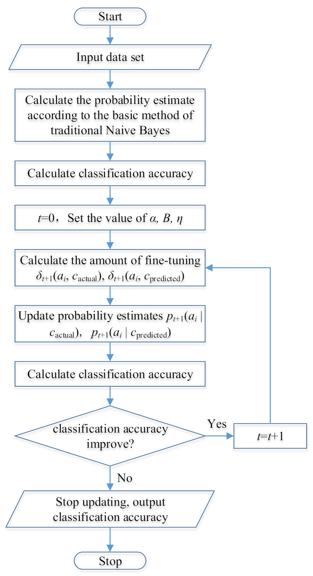
2. Fine-Tuning Naive Bayesian Model

The Naive Bayes classifier is based on the Bayesian rules. It calculates the probability that each sample belongs to each category according to the value of the sample attribute, and then uses the category with the highest probability as the predicted category c_predited of the new sample [21]. In this paper, the decision attributes and class variables are, respectively, {A₁, A₂, …, A_n} and {C₁, C₂, … , C_m}, where n and m respectively represent the number of sample decision attributes and the total number of sample categories, using {a₁, a₂, … , a_n} and {c₁, c₂, … , c_m} respectively represent the corresponding values. Assume that the actual class of the sample is c_actual; that is, if c_predited = c_actual, the classification is successful. The prediction category c_predited is calculated as follows [22]:

$$c_{\mathrm{predicted}}=\underset{c_j\in C}{\arg \max }\frac{p(a_1,a_2,\dots ,a_n|c_j)\cdot p(c_j)}{p(a_1,a_2,\dots ,a_n)}$$

(1)

where, p(c_j) is the prior probability of each class, c_j. p(a₁, a₂, … , a_n|c_j) is the probability that A₁, A₂, … , A_n take values a₁, a₂,…, a_n under the condition of the category c_j.

In the given actual calculation example, the probability p(a₁, a₂, … , a_n) is the same, so Equation (1) can be written as:

$$c_{\mathrm{predicted}}=\underset{c_j\in C}{\arg \max } p(a_1,a_2,\dots ,a_n|c_j)\cdot p(c_j)$$

(2)

The Naive Bayes algorithm assumes that the decision attributes of the samples are independent of each other:

$$p(a_1,a_2,\dots ,a_n|c_j)={\displaystyle \prod _{i=1}^{n}p(a_i|c_j)}$$

(3)

Therefore, Equation (2) can be rewritten as:

$$c_{\mathrm{predicted}}=\underset{c_j\in C}{\arg \max } p(c_j)\cdot {\displaystyle \prod _{i=1}^{n}p(a_i|c_j)}$$

(4)

The Naive Bayes classifier has shown excellent accuracy in many fields. However, its accuracy is highly dependent on good probability estimates—namely, p(c_j) and p(a₁, a₂, … , a_n|c_j). Therefore, if the sample training data that need to be predicted are very few, the traditional Naive Bayes classification effect is not ideal [23]. For this reason, this research proposes a fine-tuning Naive Bayes model to improve the classification accuracy of the Naive Bayes classifier.

The fine-tuning Naive Bayes model proposed in this paper includes two stages. In the first stage, the probability estimate is calculated according to the basic method of traditional Naive Bayes. In the second stage, the probability estimates are fine-tuned.

If the Naive Bayes classifier incorrectly classifies the training samples, it means that given the decision attribute values a₁, a₂, …, a_n of the sample, the value of the predicted class probability c_predited is higher than the sample’s actual class probability c_actual. Therefore, we need to increase the probability estimate required to calculate the actual class probability and reduce the probability estimate required to calculate the predicted class probability. That is, increase p(a_i|c_actual) and decrease p(a_i|c_predited) to reduce the probability of incorrect prediction c_predited. The fine-tuning equation is as follows [24]:

$$p_{t+1}(a_i|c_{\mathrm{actual}})=p_t(a_i|c_{\mathrm{actual}})+{\delta }_{t+1}(a_i,c_{\mathrm{actual}})$$

(5)

$$p_{t+1}(a_i|c_{\mathrm{predicted}})=p_t(a_i|c_{\mathrm{predicted}})-{\delta }_{t+1}(a_i,c_{\mathrm{predicted}})$$

(6)

where t is the number of cycles. As long as the classification accuracy is improved each time, the parameters will be fine-tuned.

The amount of fine adjustment δ is proportional to the amount of error. The error calculation equation is as follows:

$$error=\left|p_0(c_{\mathrm{actual}})-p_0(c_{\mathrm{predicted}})\right|$$

(7)

where, p₀(c_actual) and p₀(c_predited) are the normalized actual class probability and predicted class probability, respectively. The normalized equation is as follows:

$$p_0(c_j)=\frac{p(c_j)}{{\displaystyle {\sum }_{k=1}^{m}p(c_k)}}$$

(8)

In addition, as the probability value of the actual decision attribute p(a_i|c_actual) decreases, the amount of fine-tuning should increase. This is because the smaller the probability value of the actual decision attribute, the more likely it is to cause the final classification error. This paper sets the probability difference of actual decision attributes as follows:

$$\alpha \cdot p(ma{x}_i|c_{\mathrm{actual}})-p(a_i|c_{\mathrm{actual}})$$

(9)

where, max_i is the i-th decision attribute with the largest probability value. This formula can ensure that the larger p(a_i|c_actual), the smaller the amount of fine-tuning. α is a constant greater than or equal to 1, and is taken as 2 in this paper.

On the contrary, as the probability value of the predictive decision attribute p(a_i|c_actual) decreases, the amount of fine-tuning should decrease. This is because the greater the probability value of the predictive decision attribute, the more likely it is to cause the final classification error. This paper sets the probability difference of predicted decision attributes as follows:

$$\beta \cdot p(a_i|c_{\mathrm{predicted}})-p(mi{n}_i|c_{\mathrm{predicted}})$$

(10)

where, min_i is the i-th decision attribute with the smallest probability value. This formula can ensure that the larger p(a_i | c_predited), the larger the amount of fine-tuning. β is a constant greater than or equal to 1, and is taken as 2 in this paper.

The fine-tuning equation can be rewritten as:

$${\delta }_{t+1}(a_i,c_{\mathrm{actual}})=\eta \cdot (\alpha \cdot p(ma{x}_i|c_{\mathrm{actual}})-p(a_i|c_{\mathrm{actual}}))\cdot error$$

(11)

$${\delta }_{t+1}(a_i,c_{\mathrm{predicted}})=\eta \cdot (\beta \cdot p(a_i|c_{\mathrm{predicted}})-p(mi{n}_i|c_{\mathrm{predicted}}))\cdot error$$

(12)

where, η is a constant between 0 and 1, which controls the amplitude of the fine-tuning, and is taken as 0.01 in this paper.

The process of fine-tuning the Naive Bayes model is shown in Figure 1.

3. Fault Diagnosis Method of PV Arrays Based on FTNB

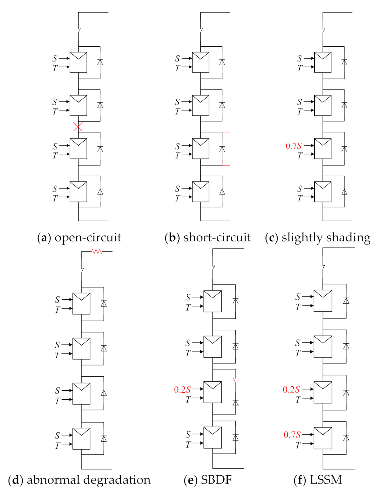
3.1. Description of PV Arrays Fault Problem

The fault diagnosis model of PV arrays based on the FTNB proposed in this paper is shown in Figure 2, including a typical PV grid-connected system and the proposed fault diagnosis method based on FTNB.

A typical PV system mainly includes PV arrays and grid-connected inverters. At present, the grid-connected inverters produced on the market are equipped with a Maximum Power Point Tracking (MPPT) function and can collect Maximum Power Point (MPP) data regularly [25]. The output characteristics of the PV array are non-linear under normal or fault conditions. When the PV array fails, its structure changes, resulting in a change in the output characteristic curve and a decrease in the MPP. However, even if the fault is not repaired, the PV inverter is likely to continue to operate, as long as the PV array can reach the minimum voltage for inverter operation. At this time, the PV system will operate at a new voltage, but lower than the MPP under normal conditions [26]. In this paper, the change of the MPP of the PV array is used for fault diagnosis.

The fault diagnosis method proposed in this paper can be integrated into the PV inverter. The inputs of this method are the MPP data of the inverter and the open-circuit voltage and short-circuit current of the simulation model. The input of the simulation model is the irradiance and temperature monitored by the weather station installed in the PV power station. Therefore, the method does not need to install additional measuring devices and only requires DC-side data, which is easy to implement.

Common PV array failures include open-circuit fault, short-circuit fault, partial shading, and abnormal degradation [27,28].

Open-circuit fault: Open-circuit faults in PV strings are caused by many reasons, such as PV cell damage, cable damage, and connector aging. This fault will reduce the output current due to the reduction of the branch circuit, thereby greatly reducing the output power.

This paper simulates the I-V curves of two kinds of open-circuit faults, i.e., one and two string open-circuit faults of the PV array. The normal and fault I-V curves are shown in Figure 3. It is obvious that due to the emergence of the open-circuit fault, the short-circuit current and maximum power decreased sharply, while the open-circuit voltage remains unchanged.

Short-circuit fault: Short-circuit faults are caused by an accidental connection between two nodes of the PV array. The reasons for this failure are insulation aging or damage, water in the junction box, or lightning current that burns the insulator. This fault will cause the faulty string voltage to decrease, resulting in a significant decrease in output power.

This paper simulates the I-V curves of two kinds of short-circuit faults, i.e., one and two components in a series of PV arrays are short-circuited respectively. The normal and fault I-V curves are shown in Figure 4. It is obvious that as the short-circuit fault occurs, the open-circuit voltage and maximum power greatly decrease, while the short-circuit current remains unchanged.

Partial shading: The partial shading fault may be caused by uneven solar radiation on the module. If some components are severely shaded, it will cause them to be reverse biased and consume power as a resistive load. The shaded components will generate heat at this time, forming hot spots, which will seriously damage the solar cells.

This paper simulates the I-V curves of two kinds of partial shading faults, i.e., 30% of one component is shaded, and 30% and 70% of two components are shaded, respectively. The normal and fault I-V curves are shown in Figure 5. It can be seen from the figure that the I-V curves of partial shading faults have multiple local peaks. This is mainly because the bypass diode of the PV module is activated under shading conditions.

Abnormal degradation: When PV modules work in an exposed environment for a long time, aging and decay are inevitable. As the service life of PV modules increases, the degree of aging gradually increases. Under normal circumstances, the annual decay rate of the modules is less than 1%. However, due to the internal defects of the PV cell, shell problems, thermal cycling, corrosive environment, and other factors, will cause abnormal degradation of the components, greatly increase the attenuation rate, and seriously reduce the output power of the PV system.

This paper simulates the I-V curves of two kinds of abnormal degradation faults, i.e., resistors of 1 Ω and 2 Ω are connected in series with the PV array, respectively. The normal and fault I-V curves are shown in Figure 6. It can be seen from the figure that the open-circuit voltage and short-circuit current of the abnormal degradation fault remain unchanged, while the maximum power is significantly decreased.

The main faults detected by the diagnostic model proposed in this paper are divided into the following six categories, including four separate fault types: open-circuit fault, short-circuit fault, slightly shading, abnormal degradation, and two mixed fault types: severe shading with faulted bypass diode (SBDF) and slight shading and severe shading mixed (LSSM). Severe shading is a condition that causes a component to be short-circuited by the bypass diode. The opposite is true for slight shading, and the shading degree cannot make the component short-circuited by the bypass diode.

The MPP data of the PV array is shown in Figure 7.

3.2. Fault Diagnosis Method

This paper adopted the FTNB to diagnose PV faults. The data required to diagnose the fault are irradiance incident on module surface, ambient temperature, MPP voltage (V_mpp), MPP current (I_mpp), and maximum power (P_mpp).

In order to improve the data clustering degree and the recognition accuracy, the decision attributes of the FTNB are selected as normalized voltage (V_norm), normalized current (I_norm), and normalized power (P_norm). The calculation of the three decision attributes is as follows:

$$\left\{\begin{array}{c}{V}_{\mathrm{norm}}=V_{\mathrm{mpp}}/V_{\mathrm{OC}}\\ I_{\mathrm{norm}}=I_{\mathrm{mpp}}/I_{\mathrm{SC}}\\ P_{\mathrm{norm}}=P_{\mathrm{mpp}}/P_{\max }\end{array}\right.$$

(13)

where, V_oc and I_sc are the open-circuit voltage and the short-circuit current of the distributed PV system under normal conditions, respectively. These two values are obtained by the PV system simulation model built in Matlab. The structure of the PV system simulation model is completely consistent with the actual PV system. The V_oc and I_sc can be obtained by only entering the irradiance and temperature monitored by the weather station installed in the PV power station. P_max is the maximum output power of the PV array under standard test conditions

The normalized data of the PV array is shown in Figure 8.

The specific steps for fault diagnosis are as follows:

Step 1: Collect model training samples. Collect training samples for normal and six fault conditions of the PV array, each including irradiance, temperature, V_mpp, I_mpp, P_mpp.

Step 2: Establish a simulation model of the PV array. Establish the same simulation model as the actual PV array in MATLAB/Simulink.

Step 3: Obtain open circuit voltage and short circuit current. Input the irradiance and temperature data of the training samples into the simulation model to obtain the corresponding V_oc and I_sc.

Step 4: Data normalization. According to the Equation (13), V_norm, I_norm, and P_norm of the training samples are obtained.

Step 5: Set the FTNB decision attributes as V_norm, I_norm, and P_norm, and the class variables are the normal state and the six fault states.

Step 6: Use the training set samples to estimate the probability according to the traditional Naive Bayes method.

Step 7: According to the FTNB process in Figure 1, set the fine-tuning parameters, and use the FTNB to fine-tune the probability estimates.

Step 8: The fault detection and diagnosis model training has been completed until the FTNB process loop stops.

Step 9: Integrate the trained fault detection and diagnosis model based on FTNB into the distributed PV inverter.

Step 10: Obtain the real-time monitoring data of the PV array. Record monitoring data every 15 min, including irradiance, temperature, V_mpp, I_mpp, P_mpp.

Step 11: Use the model integrated in the inverter to detect and diagnose the real-time monitoring data.

4. Experimental Verification

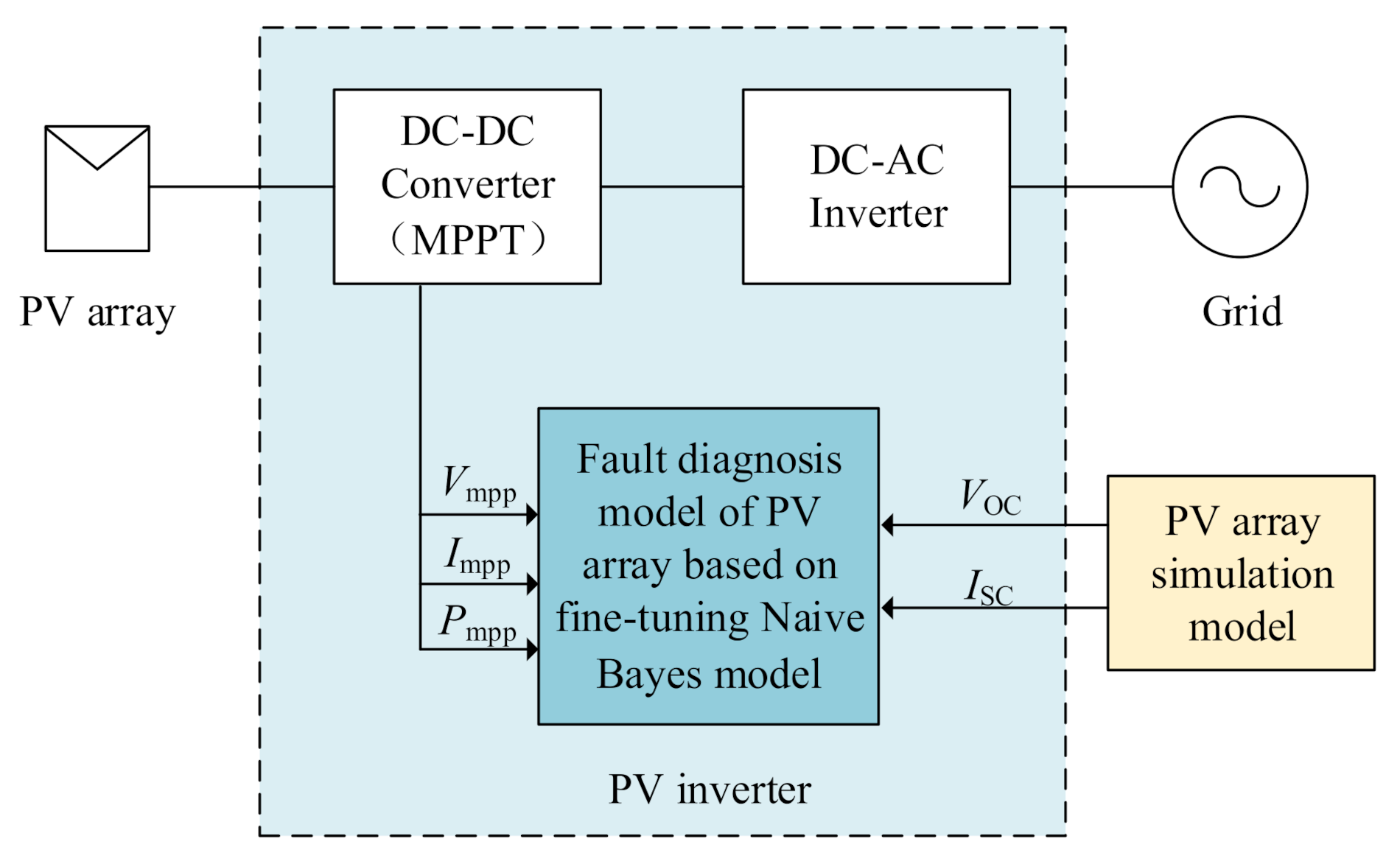
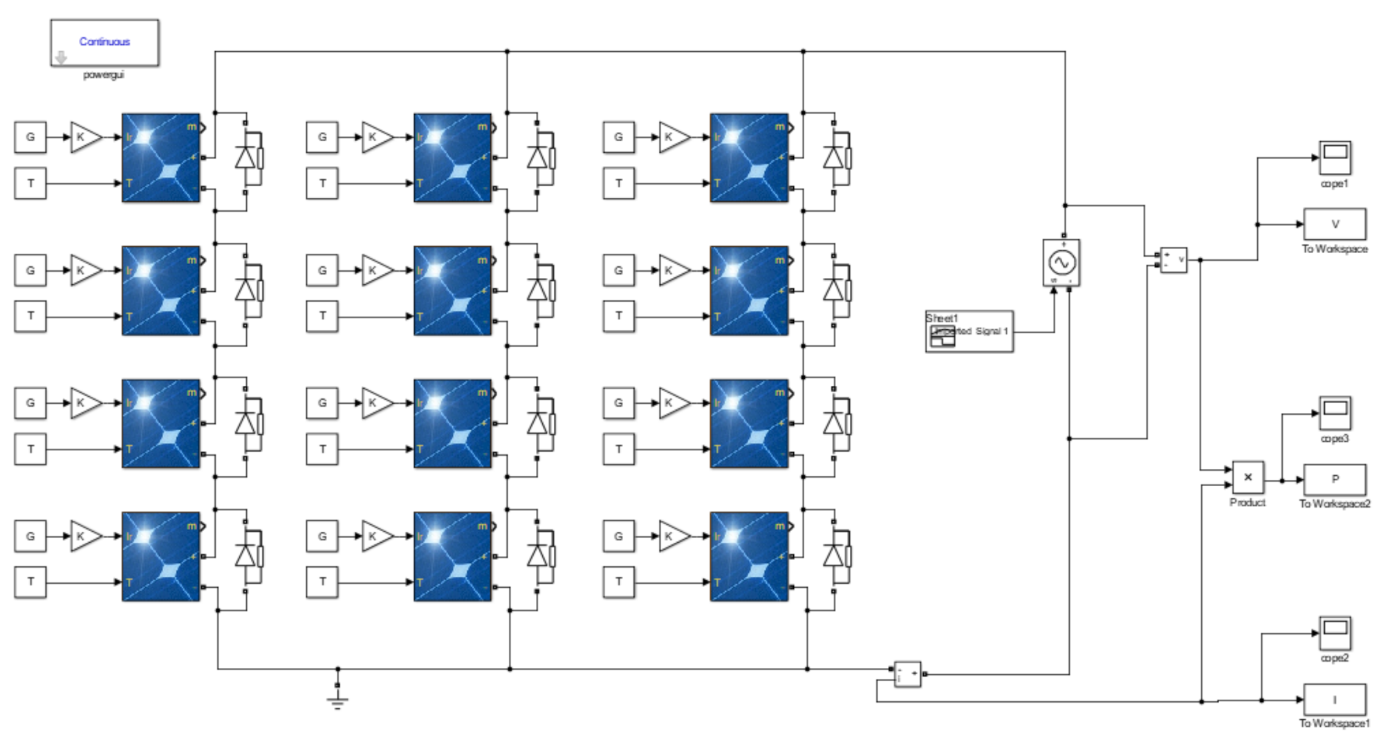
4.1. PV System Modeling

In this paper, a PV system model is built in MATLAB/Simulink to simulate different types of faults in the PV array. As shown in Figure 9, the PV system includes 12 PV modules with a rated power of 175 W. The PV array is divided into three strings, all connected to the input of the inverter, each string is composed of four PV modules in series. Each PV module can independently adjust the irradiance and temperature on the input side and are equipped with bypass diodes, and the gain module is used to adjust the degree of shading of the PV module. The main parameters of PV modules under standard test conditions (STC) are: rated power 175 W, open-circuit voltage 29.4 V, short-circuit current 7.82 A, MPP voltage 24.2 V, MPP current 7.25 A.

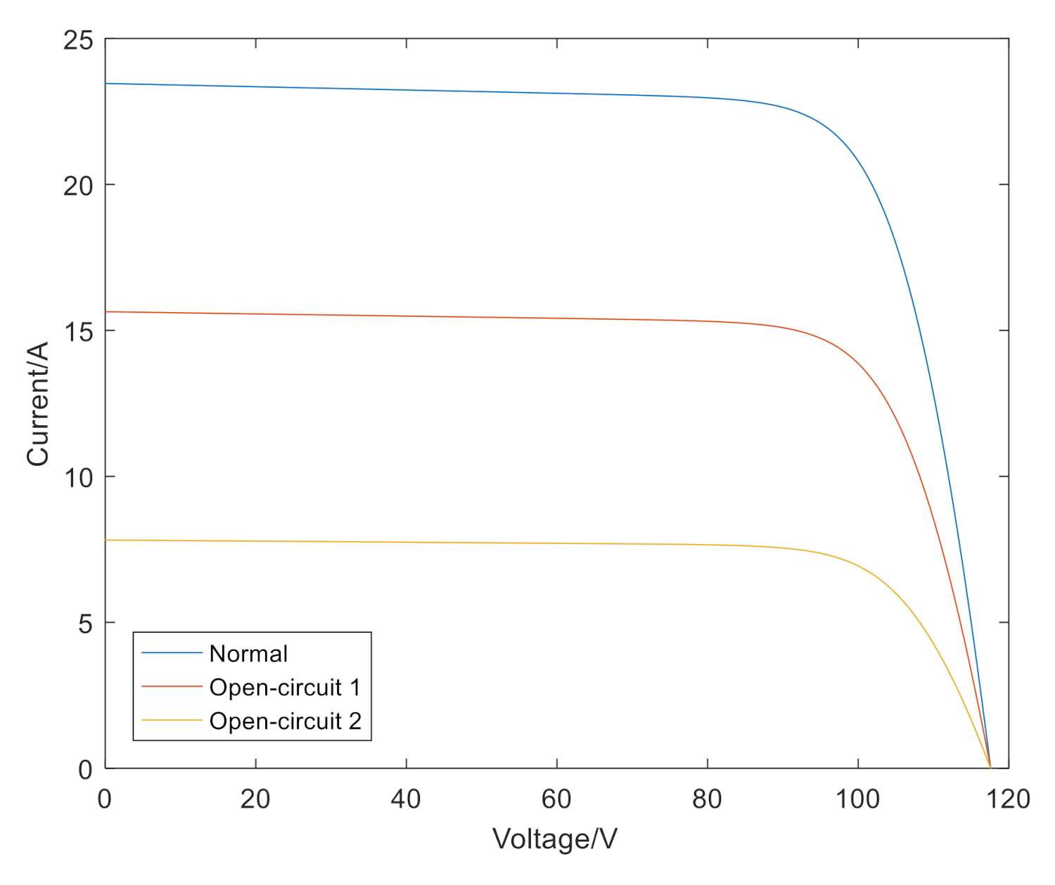
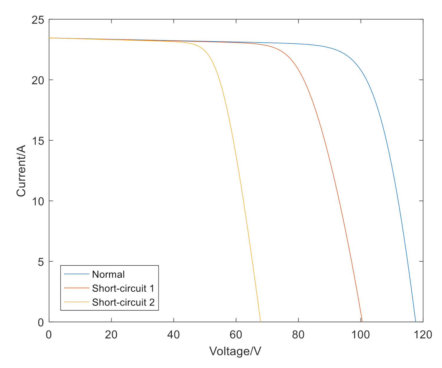
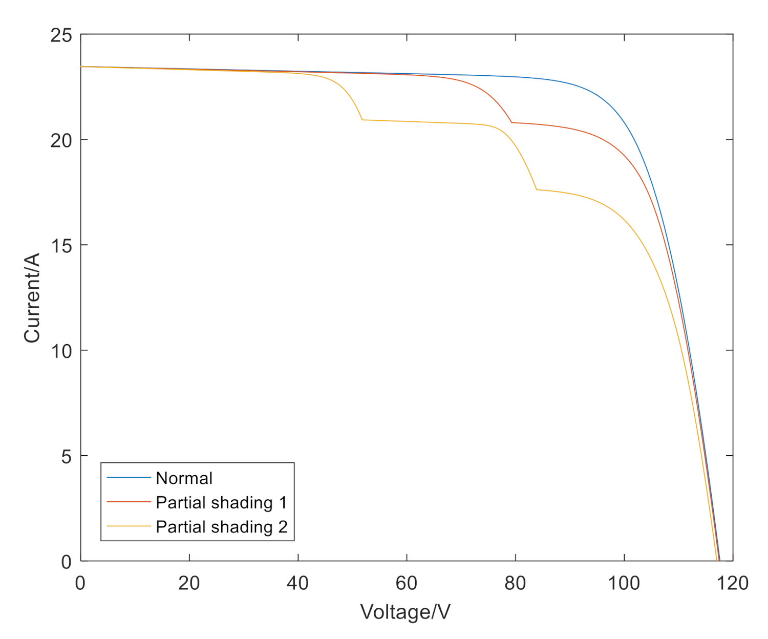
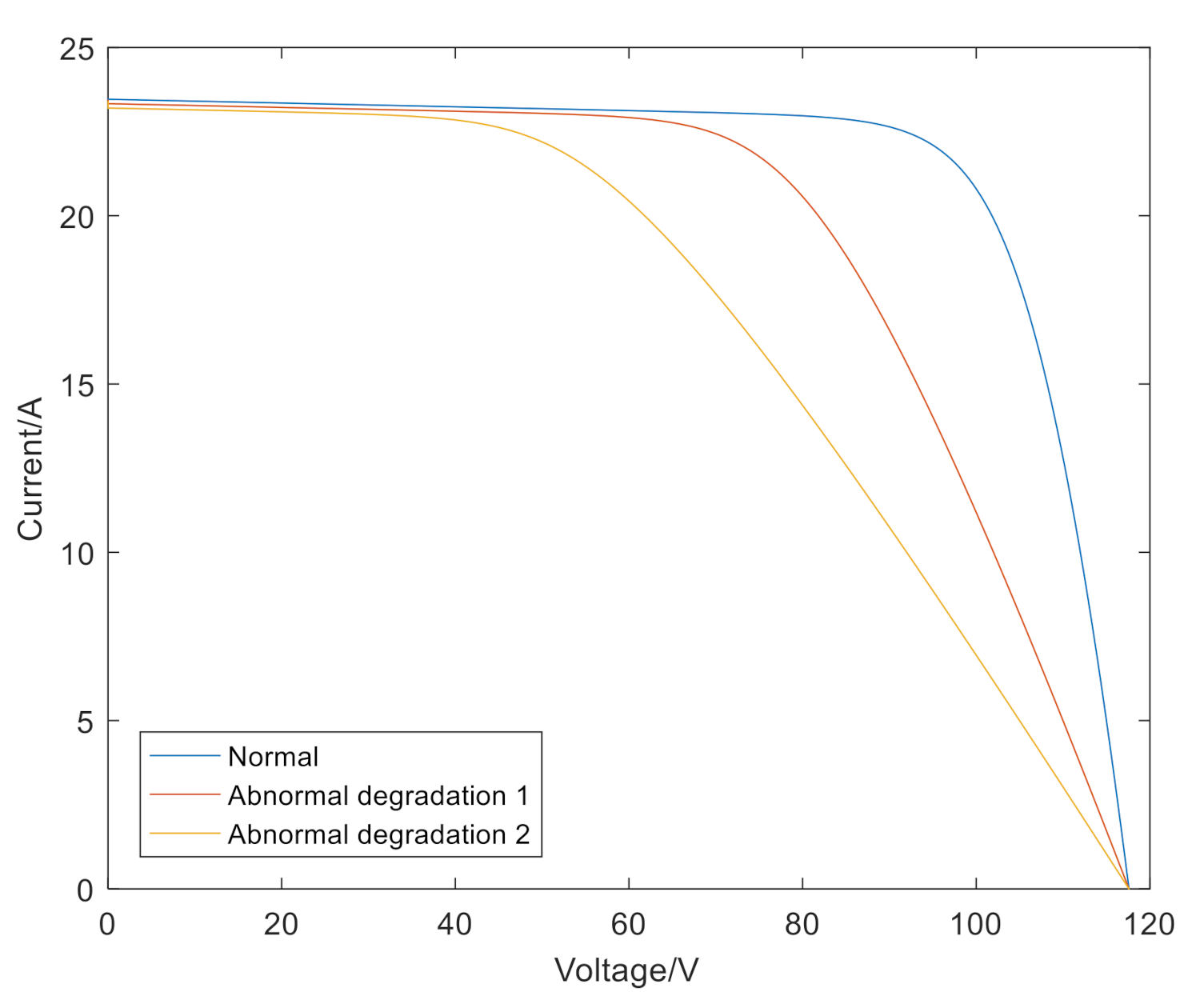
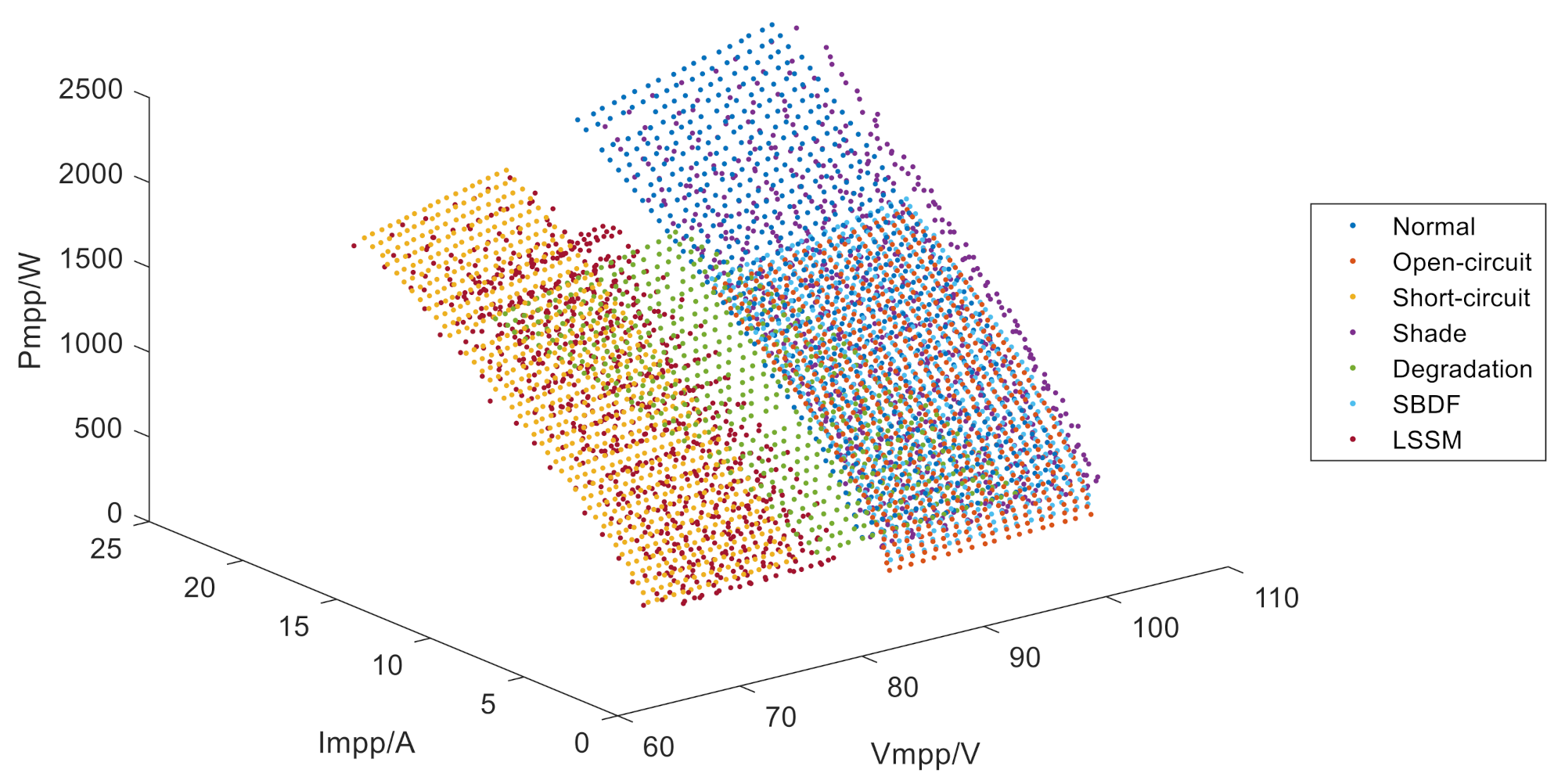
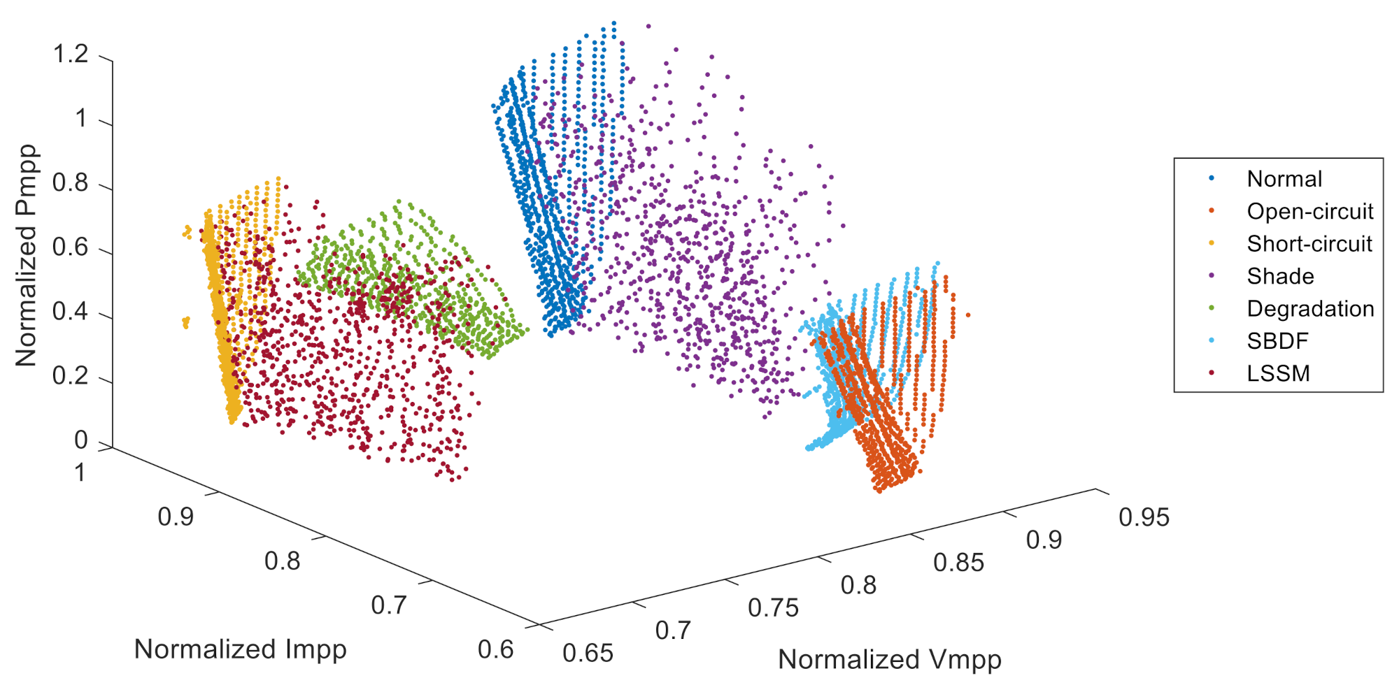
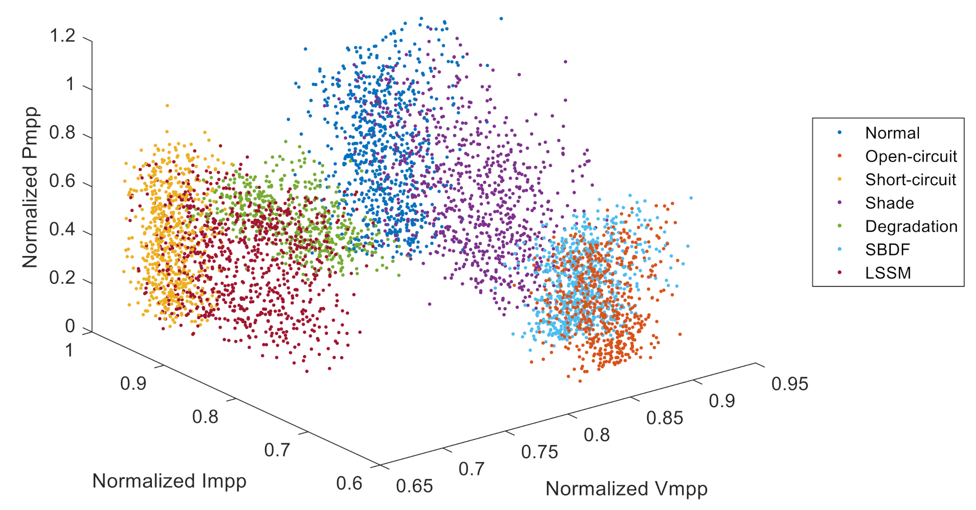
4.2. Fault Data Description

The simulation of different faults is shown in Figure 10.

Under different irradiance and temperature conditions, the normal state and six fault states of the PV array are simulated. The fault states include four separate fault types: open-circuit, short-circuit, slightly shading and abnormal degradation, and two mixed fault types: SBDF and LSSM.

The severe shading used in this paper is to reduce the light transmittance of a single component to 20%; that is, the input irradiance of the component becomes 20% of the normal component. The light transmittance of the slightly shaded module is reduced to a random value; the value range is 70–90%, which is randomly selected during each simulation. The simulation method for abnormal degradation is to connect a 2 Ω resistor in series with the PV string. In order to cover all working conditions as much as possible, the data are collected under a wide range of environmental conditions during the simulation: the range of irradiance is 200–1000 W/m², with a step size of 20 W/m²; the range of temperature is 6–40 °C, with a step size of 2 °C. The total amount of data collected in each state is 738. The collected values under normal and fault conditions are plotted in Figure 7.

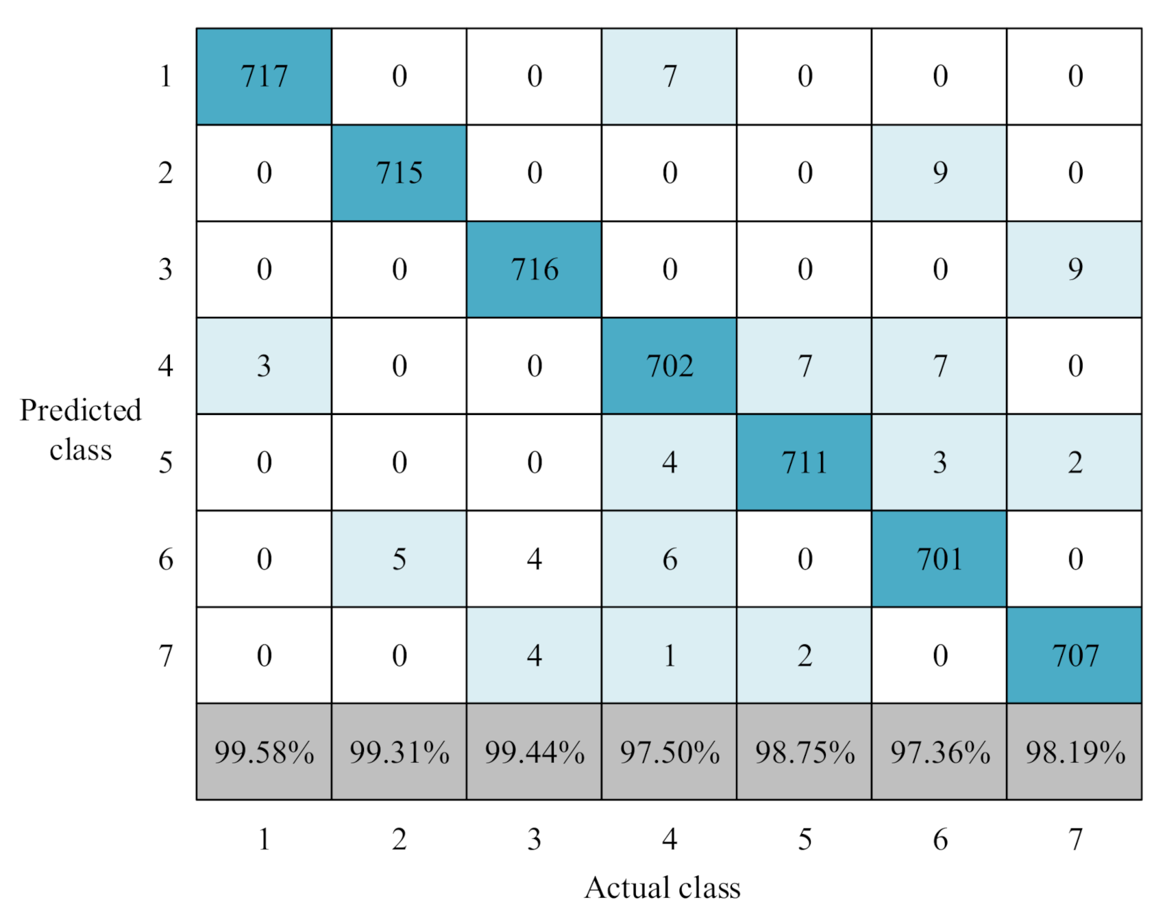
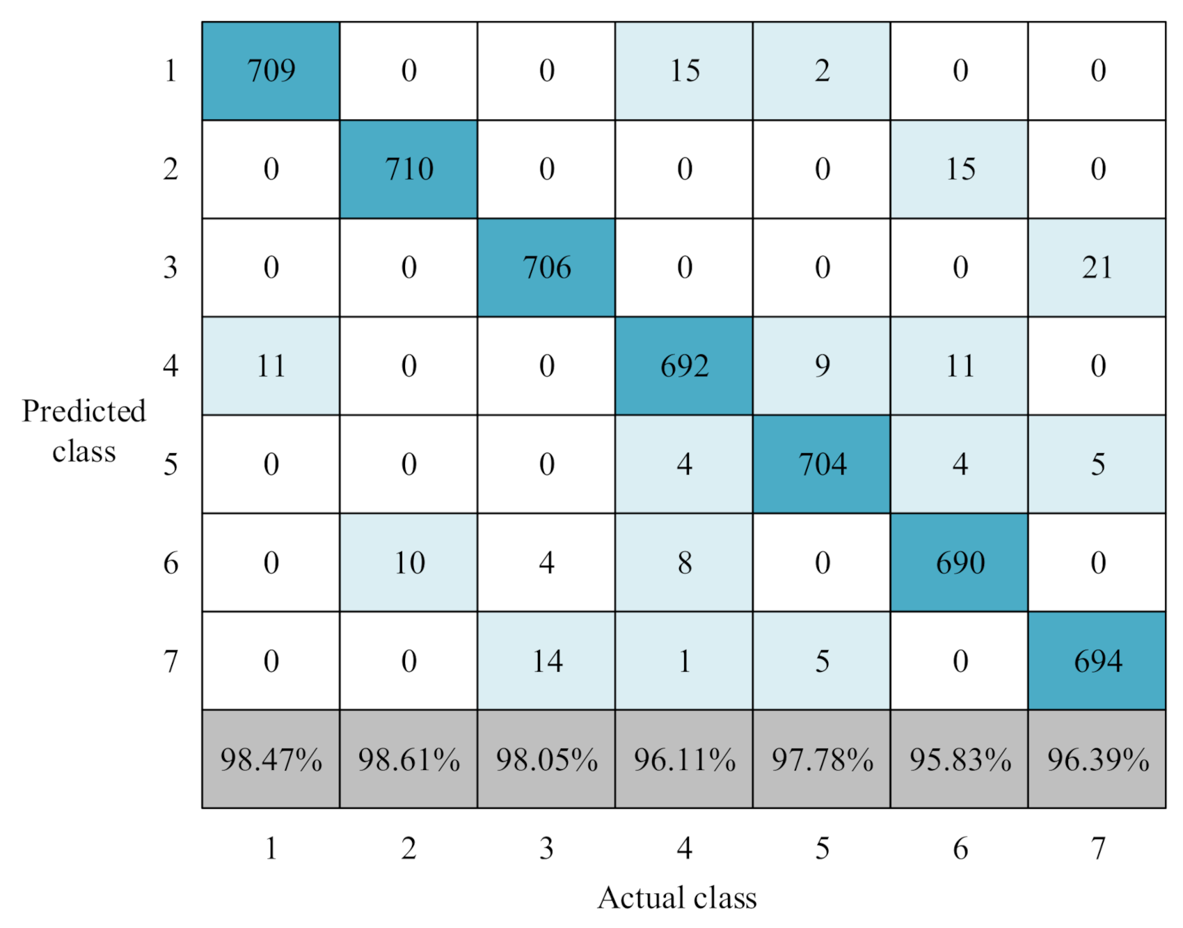
4.3. Simulation Result with the Ideal Data

In view of the small number of PV fault samples in actual operation, this paper selected only 18 data from each type of fault as training samples (accounting for 2.44% of the total data volume of each type of fault), and the rest of the collected data were used as test samples.

In order to better compare the advantages of the fine-tuning Naive Bayes model, this paper uses the Naive Bayes model and the fine-tuning Naive Bayes model to diagnose PV array faults. First, use the training samples to train the two models separately. Second, input the test data into the two models one by one for fault diagnosis.

This paper uses a confusion matrix to show the fault diagnosis test results of the two models, as shown in Figure 11 and Figure 12. Numbers 1–7 represent different classes: Class 1: normal, Class 2: open-circuit, Class 3: short-circuit, Class 4: slightly shading, Class 5: abnormal degradation, Class 6: SBDF, Class 7: LSSM.

The dark blue box represents the amount of data correctly classified for each class. For example, the dark blue box in the first column of Figure 11 indicates that 717 of the 720 test data of Class 1 are correctly classified. The light blue box represents the amount of misclassified data. For example, the fourth light blue box in the first column of Figure 11 indicates that 3 of 720 test data in category 1 are incorrectly classified as Class 4. The gray box represents the accuracy of classification for each class. For example, the gray box at the bottom of the first column in Figure 11 represents that 99.58% of the test samples in Class 1 are correctly classified.

It can be seen from the figures that the fault diagnosis accuracy based on the Naive Bayes model is 93.27%, and the fault diagnosis accuracy based on FTNB is 98.59%. Compared with the Naive Bayes model, the FTNB proposed in this paper is more effective.

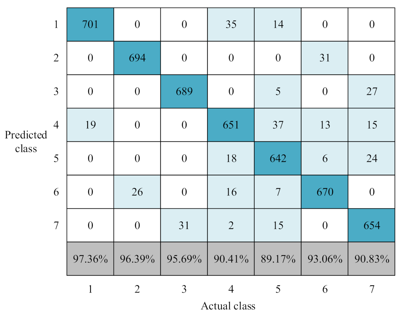
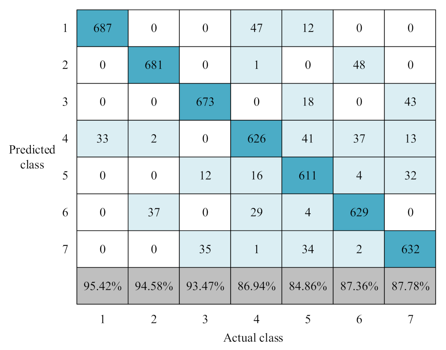
4.4. Simulation Result with the Noise Data

In practice, the irradiance and temperature are not controllable, and the fail experiment may cause safety hazards and even cause permanent damage to the PV system [29]. Therefore, the data used in this paper are obtained through simulation. However, in practice, due to the influence of factors such as the error of the measuring device and the drift of the sensor, the data collected always have a certain degree of noise. Therefore, in order to test the applications of the proposed method in the real field, this paper created noise data. The equation for obtaining noise data is as follows [30]:

$$D_{noise}=D_{ideal}\times (1+(\alpha +\beta \times \mathrm{randn}\left)\right)$$

(14)

where, D_noise is the noise data, and D_ideal is the ideal data; α is the average value of the noise signal; β is the standard deviation of the noise signal; randn is a function provided by Matlab to generate data that obeys the normal distribution. In this paper, α = 0 and β = 0.01. The normalized noise data are shown in Figure 13.

Same as the simulation of ideal data, this paper still selected only 18 data from each type of noise data as training samples, and the rest of the noise data were used as test samples. The fault diagnosis test results with noise data are shown in Figure 14 and Figure 15.

It can be seen from the figures that in the case of considering the data noise, the fault detection and diagnosis method based on the FTNB still has a high accuracy rate with 97.32%. This reflects the effectiveness and reliability of the method in the real field. Compared with the Naive Bayesian method, the FTNB still has higher accuracy.

In order to verify the advancement and efficiency of the proposed method, this research compared the results of the proposed method’s fault diagnosis on noise data with the results of the other eight methods. These methods were: SVM [17], expectation–maximization (EM) [17], agglomerative clustering (AG) [17], K-means [17], Birch [17], mean–shift (MS) [17], ANN [30], and PNN [30]. The comparison results are shown in

Table 1. The comparison results of the fault diagnosis methods.

Method	Number of Fault Types	Fault Diagnosis Accuracy/%
FTNB	6	97.32
SVM [17]	3	94.87
EM [17]	3	75.43
AG [17]	3	82.07
K-means [17]	3	54.67
Birch [17]	3	39.16
MS [17]	3	55.13
ANN [30]	2	76.63
PNN [30]	2	98.19

.

In [17], six methods are used to diagnose three types of faults: one string open-circuit fault, one module short-circuit, and three module short-circuit fault and temporary shading fault. In [30], two methods are used to diagnose two types of faults: one string open-circuit fault, three module short-circuit, and ten module short-circuit fault. The average diagnostic accuracies are listed in Table 1. It is worth mentioning that compared with the PNN method, the more complex fault types in this paper affect the accuracy of FTNB, but the difference is quite modest. Overall, the fault diagnosis method proposed in this paper is more advantageous and efficient.

5. Conclusions

In this research, a distributed PV fault diagnosis method based on a fine-tuning Naive Bayes model was proposed. This method can effectively diagnose the normal state of PV arrays, as well as open-circuit, short-circuit, slight shading, abnormal degradation, SBDF, and LSSM. The proposed distributed PV fault diagnosis method only needs to use the existing maximum power point data and meteorological data of the PV system and does not need to install additional measuring devices. It is economical and is suitable for online real-time monitoring of a distributed PV system. The fine-tuning Naive Bayes model proposed in this paper is more suitable for situations with a small number of training samples. Compared with the traditional Naive Bayes model, the method has higher classification accuracies, which are 98.59% with the ideal data and 97.32% with the noise data.

Since the working state of a short-circuit fault is basically the same as the severe shading fault, this research cannot directly identify these two, which is a direction that needs to be studied and improved. In addition, this line of research will study the application of artificial intelligence methods such as machine learning or neural networks in fault diagnosis algorithms to further improve the diagnosis accuracy.

References

1. Triki-Lahiani, A.; Abdelghani, A.B.B.; Slama-Belkhodja, I. Fault detection and monitoring systems for photovoltaic installations: A review. Renew. Sustain. Energy Rev. 2018, 82, 2680–2692. [Google Scholar] [CrossRef]
2. National Energy Administration. Grid-Connected Operation of Photovoltaic Power Generation in 2019. 2020. Available online: http://www.nea.gov.cn/2020-02/28/c_138827923.htm (accessed on 28 February 2020).
3. Green, M.A.; Emery, K.; Hishikawa, Y. Solar cell efficiency tables (version 46). Prog. Photovolt. 2015, 23, 805–812. [Google Scholar] [CrossRef]
4. Spertino, F.; Chiodo, E.; Ciocia, A.; Malgaroli, G.; Ratclif, A. Maintenance Activity, Reliability, Availability, and Related Energy Losses in Ten Operating Photovoltaic Systems up to 1.8 MW. IEEE Trans. Ind. Appl. 2020, 57, 83–93. [Google Scholar] [CrossRef]
5. Gonzalo, A.P.; Marugán, A.P.; Márquez, F.P.G. Survey of maintenance management for photovoltaic power systems. Renew. Sustain. Energy Rev. 2020, 134, 110347. [Google Scholar] [CrossRef]
6. Villarini, M.; Cesarotti, V.; Alfonsi, L.; Introna, V. Optimization of photovoltaic maintenance plan by means of a FMEA approach based on real data. Energy Convers. Manag. 2017, 152, 1–12. [Google Scholar] [CrossRef]
7. Daliento, S.; Chouder, A.; Guerriero, P. Monitoring, diagnosis, and power forecasting for photovoltaic fields: A review. Int. J. Photoenergy 2017, 54, 690–700. [Google Scholar] [CrossRef]
8. Li, Y.; Ding, K.; Chen, F.; Ding, H. Fault diagnosis of photovoltaic array based on fast oversampling principal component analysis method. Power Syst. Technol. 2019, 43, 308–315. [Google Scholar]
9. Wang, J.Y.; Qian, Z.; Zareipour, H.; Pei, Y.; Wang, J.-Y. Performance assessment of photovoltaic modules using improved threshold-based methods. Sol. Energy 2019, 190, 515–524. [Google Scholar] [CrossRef]
10. Silvestre, S.; da Silva, M.A.; Chouder, A. New procedure for fault detection in grid connected PV systems based on the evaluation of current and voltage indicators. Energy Convers. Manag. 2014, 86, 241–249. [Google Scholar] [CrossRef]
11. Dhimish, M.; Holmes, V.; Mehrdadi, B. Diagnostic method for photovoltaic systems based on six layer detection algorithm. Electr. Power Syst. Res. 2017, 151, 26–39. [Google Scholar] [CrossRef]
12. Silvestre, S.; Chouder, A.; Karatepe, E. Automatic fault detection in grid connected PV systems. Sol. Energy 2013, 94, 119–127. [Google Scholar] [CrossRef]
13. Spataru, S.; Sera, D.; Kerekes, T.; Teodorescu, R. Diagnostic method for photovoltaic systems based on light I–V measurements. Sol. Energy 2015, 119, 29–44. [Google Scholar] [CrossRef]
14. Hachana, O.; Tina, G.M.; Hemsas, K.E. PV array fault DiagnosticTechnique for BIPV systems. Energy Build. 2016, 126, 263–274. [Google Scholar] [CrossRef]
15. Hussain, M.; Dhimish, M.; Titarenko, S.; Mather, P. Artificial neural network based photovoltaic fault detection algorithm integrating two bi-directional input parameters. Renew. Energy 2020, 155, 1272–1292. [Google Scholar] [CrossRef]
16. Chen, L.; Han, W.; Zhang, J. Fault diagnosis of photovoltaic modules based on data fusion. Power Syst. Technol. 2017, 41, 170–179. [Google Scholar]
17. Harrou, F.; Dairi, A.; Taghezouit, B.; Sun, Y. An unsupervised monitoring procedure for detecting anomalies in photovoltaic systems using a one-class Support Vector Machine. Sol. Energy 2019, 179, 48–58. [Google Scholar] [CrossRef]
18. Madeti, S.R.; Singh, S.N. Modeling of PV system based on experimental data for fault detection using kNN method. Sol. Energy 2018, 173, 139–151. [Google Scholar] [CrossRef]
19. Chine, W.; Mellit, A.; Lughi, V. A novel fault diagnosis technique for photovoltaic systems based on artificial neural networks. Renew. Energy 2016, 90, 501–512. [Google Scholar] [CrossRef]
20. Chen, Z.; Wu, L.; Cheng, S. Intelligent fault diagnosis of photovoltaic arrays based on optimized kernel extreme learning machine and IV characteristics. Appl. Energy 2017, 204, 912–931. [Google Scholar] [CrossRef]
21. Yang, L.; Cao, C.; Sun, J.; Zhang, L. Research on Improved Naive Bayes Algorithm in Spam Filtering. J. Commun. 2017, 38, 140–148. [Google Scholar]
22. Di, P.; Duan, L. A new Naive Bayesian text classification algorithm. Data Collect. Process. 2014, 29, 71–75. [Google Scholar]
23. El Hindi, K. Fine tuning the Naïve Bayesian learning algorithm. AI Commun. 2014, 27, 133–141. [Google Scholar] [CrossRef]
24. Diab, D.M.; El Hindi, K.M. Using differential evolution for fine tuning naïve Bayesian classifiers and its application for text classification. Appl. Soft Comput. 2017, 54, 183–199. [Google Scholar] [CrossRef]
25. Belkaid, A.; Colak, I.; Isik, O. Photovoltaic maximum power point tracking under fast varying of solar radiation. Appl. Energy 2016, 179, 523–530. [Google Scholar] [CrossRef]
26. Zhao, Y.; Ball, R.; Mosesian, J.; Lehman, B. Graph-based semi-supervised learning for fault detection and classification in solar photovoltaic arrays. IEEE Trans. Power Electron. 2014, 30, 2848–2858. [Google Scholar] [CrossRef]
27. Mellit, A.; Tina, G.M.; Kalogirou, S.A. Fault detection and diagnosis methods for photovoltaic systems: A review. Renew. Sustain. Energy Rev. 2018, 91, 1–17. [Google Scholar] [CrossRef]
28. Fazai, R.; Abodayeh, K.; Mansouri, M. Machine learning-based statistical testing hypothesis for fault detection in photovoltaic systems. Sol. Energy 2019, 190, 405–413. [Google Scholar] [CrossRef]
29. Appiah, A.Y.; Zhang, X.; Ayawli, B.B.K.; Kyeremeh, F. Long short-term memory networks based automatic feature extraction for photovoltaic array fault diagnosis. IEEE Access 2019, 7, 30089–30101. [Google Scholar] [CrossRef]
30. Garoudja, E.; Chouder, A.; Kara, K.; Silvestre, S. An enhanced machine learning based approach for failures detection and diagnosis of PV systems. Energy Convers. Manag. 2017, 151, 496–513. [Google Scholar] [CrossRef] [Green Version]
Figure 1. Flow chart of the fine-tuning Naive Bayes model.
Energies 14 04140 g001
Figure 2. Fault diagnosis model of PV array based on FTNB.
Energies 14 04140 g002
Figure 3. I-V curves of the PV array in case of the open-circuit faults.
Energies 14 04140 g003
Figure 4. I-V curves of the PV array in case of the short-circuit faults.
Energies 14 04140 g004
Figure 5. I-V curves of the PV array in case of the partial shading faults.
Energies 14 04140 g005
Figure 6. I-V curves of the PV array in case of the abnormal degradation faults.
Energies 14 04140 g006
Figure 7. The MPP data of PV array under normal and fault conditions.
Energies 14 04140 g007
Figure 8. The normalized MPP data of PV array under normal and fault conditions.
Energies 14 04140 g008
Figure 9. PV array model.
Energies 14 04140 g009
Figure 10. Simulation models for different faults.
Energies 14 04140 g010
Figure 11. Fault diagnosis result with ideal data based on the FTNB.
Energies 14 04140 g011
Figure 12. Fault diagnosis result with ideal data based on the Naive Bayesian method.
Energies 14 04140 g012
Figure 13. The normalized noise data under normal and fault conditions.
Energies 14 04140 g013
Figure 14. Fault diagnosis result with noise data based on the FTNB.
Energies 14 04140 g014
Figure 15. Fault diagnosis result with noise data based on the Naive Bayesian method.
Energies 14 04140 g015