Optimal Computation of Network Indicators for Electricity Market Bidding Zones Configuration Considering Explicit N-1 Security Constraints ^†

Abstract

In this paper an optimization problem designed to calculate electric grid specific indicators to be used within model-based methodologies for the definition of alternative electricity market bidding zone configurations is designed. The approach integrates within the framework of a bidding zone review process aligned to the specifications of the Commission Regulation (EU) 2015/1222 (CACM) and Regulation (EU) 2019/943 of the European Parliament and of the Council (CEP). The calculated solution of the optimization provides locational marginal prices and allows to determine, outside the optimization problem, the power transfer distribution factors for critical elements. Both indicators can be used as inputs by specially designed clustering algorithms to identify model-based electricity market bidding zone configurations, as alternative to the current experience-based configurations. The novelty of the optimization problem studied in this paper consists in integrating the N-1 security criteria for transmission network operation in an explicit manner, rather than in a simplified and inaccurate manner, as encountered in the literature. The optimization problem is evaluated on a set of historical and significant operating scenarios of the Italian transmission network, carefully selected by the Italian transmission system operator. The results show the optimization problem capability to produce insightful results for supporting a bidding zone review process and its advantages with respect to simplified methodologies encountered in the literature.

1. Introduction

The European electricity market is on a straight road towards a liberalized and integrated European market: full integration of the day-ahead European market has already been implemented [1] while clear roadmaps are defined for the integration of the intra-day [2] and balancing markets [3]. The main goals of this process are: (i) maximizing social welfare; (ii) optimally integrating renewable energy sources; (iii) maximizing cross-border trade opportunities; (iv) providing competitive energy prices [4]. To identify the optimal market clearing solution for these markets, complex optimization algorithms are used, e.g., [5,6] for the day-ahead market or [7] for the intra-day market.

This work focuses on the first level of the European energy market, i.e., in the day-ahead market which is a zonal market: the European transmission network is divided into several bidding zones that integrate, in a simplified manner, the relevant transmission constraints in the day-ahead market clearing algorithm, limiting the possibility of significant incompatibilities between generation schedules resulting from the market and the real-time system security, which, if present, could lead to gaming opportunities for the market participants. Thus, the bidding zones are areas of the transmission network within which the market actors can exchange energy unconstrainted by the transmission network, while the energy transferred between these areas is limited to the available capacity evaluated using methodologies specified by the CACM.

Therefore, within European energy markets the transmission grid is represented through bidding zones connected by equivalent interconnectors where the energy flow is limited by the available transmission capacity. In these circumstances, the market clearing solution is strongly influenced by the congestion of these interconnectors [5,6,7] leading to the conclusion that the bidding zone review process is an important activity where network operation security, market efficiency and the bidding zone’s stability and robustness requirements must be properly balanced. While the security criteria could be inclined to point towards more granular bidding zone configurations, market efficiency and or stability/robustness requirements could favor configurations characterized by a reduced number of geographically large bidding zones.

Consequently, CACM established a monitoring procedure to continuously verify the ability of the bidding zone configuration presently used by the market to meet the above-mentioned goals: the European Network of Transmission System Operators for Electricity (Entso-E) publishes a technical document every three years reporting the congestions registered in the investigated period and their related costs to the transmission grid [8], while the Agency for the Cooperation of Energy Regulators (ACER) publishes a Market Monitoring Report [9], where market efficiency issues are evaluated.

If these monitoring activities find potential issues, a bidding zone configuration review process is activated. On the other hand, the process could also be initiated by transmission system operators (TSOs) or national regulators if it is thought that improvements are possible within the geographic area of their competence. Last, but not the least, it should be mentioned that the CEP regulation requires the initiation of a bidding zones configuration review process at European level right after its approval (the process is currently ongoing).

One of the key components of a bidding zone configuration review process is the definition of alternative configurations and their evaluation against the current one. For this purpose, two approaches can be adopted: (i) expert-based, that exploits the transmission network operation knowledge of the TSO, its experience, as well as on some statistical information built on actual data and/or future scenarios evaluation, and (ii), model-based, that uses specially designed mathematical models to support the TSO. In general, the model-based approaches consist of the following steps: (i) determining, by employing a complete model of the transmission network, electric grid-specific indicators related to optimal electricity market clearing and (ii) passing them as inputs to specially tailored clustering algorithms that identify the bidding zones as consistent areas of the electric grid where the specified indicators present similar values. Clearly, since a bidding zone configuration must be stable over time and over a realistic range of network operating conditions, the clustering algorithms must process a significant number of network operating conditions cases so that the identified bidding zone configuration reflects consistent over time network indicator patterns. The focus of the current work is on the first step.

Work reported in [10,11,12,13] performs a critical literature review regarding the model-based indicators, the mathematical models used to determine them and the clustering algorithms used to determine the zonal structure of transmission networks for electricity markets. A few important conclusions can be derived. In general, the most used indicators are the locational marginal price (LMP), which is defined as the marginal energy price of a bus of the electric network according to the solution of a nodal market clearing algorithm, and the power transmission distribution factor (PTDF) which is defined as the sensitivity of the variation in the power flow through a branch of the network to variations in the nodal injected power at a considered bus. To calculate these indicators, nodal market models where the electric grid is represented in detail are used. This is a very important aspect as precise identification of network congestions can only be performed on a complete model of the transmission network. Here, in general, the literature review identifies the use of DC power flow (DC PF) models to represent the grid, and the adoption of only the N security criterion, i.e., network elements outages are not explicitly considered when network indicators are calculated for the identification of alternative bidding zone configurations. The DC PF model is an approximation that neglects voltage and reactive power from the network model and, in general, this approximation is considered reasonable for HV transmission networks. However, adopting only the N security criterion is a critical aspect as, often, the unexpected outage of network elements leads to congestion of the electric branches in the grid. In practice, the N-1 security criterion, preventive or corrective, involving one network element outage (branch, generator) is adopted. Indeed, the regulators and/or the TSOs require that the electricity market is solved such that the N-1 security criterion is satisfied by the market clearing solution. For example, at European level the day-ahead and intra-day electricity market uses two approaches to manage the intra-zone flows, both specified by the CACM and both considering the N-1 security criterion: (i) the available transfer capacity (ATC) approach where the net transfer capacities on the equivalent interconnectors between two neighboring bidding zones need to include the effect of the outage of a critical network element (see Article 21 of Commission Regulation (EU) 2015/1222 of 24 July 2015) or (ii) the flow-based approach where the flows related to the set of critical branch–critical outages of main intra-zone interconnectors is explicitly considered in the market clearing algorithm through approximated linear equations for central western European countries [14].

However, in the forementioned literature review, checked for updates by the authors, a few papers indirectly consider the N-1 security criterion, while most of them do not, when it comes to the calculation of network indicators. Breuer et al. [15] models the optimization problem that calculates the LMPs with only the N security criterion, therefore only limiting the branch currents to their corresponding thermal limits. The N-1 security criterion is considered only through an economic evaluation of the corrective actions needed to mitigate the congestions in case of outages. However, the paper does not consider the length of the short-term thermal limit violation in case of outages: the violation could be so high that the congested line is tripped before corrective actions can be determined and applied. As a consequence, the network could go into cascading trips that would lead to blackouts. Bjorndal et al. [16] limit in N security operating conditions the total flow over sets of critical lines with the goal to prevent the overloading of one of these lines in case of outage of another. But the calculation of the sets power flow limits is very network specific and relies heavily on the TSO experience. Hence, it may not be generally applicable, especially if network expansion scenarios are to be considered, and it tends to be more of an expert-based approach rather than a model-based approach. Finally, another approach is to apply the N security criterion but reduce the limits of branch power flows by a percentage of the thermal limit hoping that a tighter N security limit would guarantee the satisfaction of N-1 security criterion [17,18,19] Thus, Breuer et al. [17] set the branch flow limit to 70% of the thermal limit, Burstedde [18] to 80% and Felling et al. [19] to 85%. However, there is no clear theoretical support for these values as it is not proven any of them could completely satisfy the N-1 security criteria.

Even though the N-1 security criteria has not yet been included in the mathematic models that calculates network indicators for identification of alternative bidding zone configurations, it has however been considered in the literature when solving various security constraint optimal power flow problems (SCOPF). The major difficulty of the SCOPF is its high dimensionality, especially for large systems: solving the problem directly for a large power system by imposing simultaneously all N-1 constraints, would lead to prohibitive memory and CPU time requirements. Moreover, as in real life applications most contingencies do not constrain the optimum, including them all into the SCOPF problem increases the complexity of the computations by shrinking the feasible region, and can lead to algorithmic/numerical problems. This is especially true under stressed operating conditions, i.e., when the SCOPF is most useful. Besides adopting various contingency filtering techniques [20], which are generally used in all works since the seminal work of Monticelli et al. [21], Benders decomposition (BD) [22] has been widely used to solve various SCOPF problems. Just to name a few noteworthy contributions, Monticelli et al. [21] focused on the optimal scheduling of the post-contingency corrective actions and use the DC PF to model the network, Yamin et al. [23] propose a linearized power flow model that include both congestion mitigation and voltage security in electricity market model, while Capitanescu et al. [20] solve a typical AC SCOPF also using BD. The BD approach decomposes the original SCOPF problem into a master and several slave problems that interact iteratively. It is very attractive approach as it can keep the size of the decomposed problems tractable as well as for potential use with parallel computations. On the other hand, BD solutions can still preserve a certain degree of infeasibility [23] and (theoretically) BD requires the convexity of the feasible region which cannot be guaranteed in AC SCOPF models [20]. Other approaches, like [24,25,26] formulate SCOPF models that include all network equations for the normal operating conditions and for all considered contingencies. Even for a small set of carefully filtered contingencies such an approach would generate a large size optimization model, possibly non-tractable, in case of large, realistic, transmission networks. In fact, the mentioned papers test only very small power systems. Finally, Lin et al. [27] use a standard OPF model consisting of only the constraints written for the normal operating conditions, while the N-1 operating conditions are indirectly present in the optimization model through iterative update of the normal operating conditions bounds. The approach could be promising but it does not consider the corrective actions and relies on postulating, without proof, the “coherence of steady-state with post-contingency” forgetting that some control resources (like synchronous generators) may change their behavior discreetly between steady-state and post-contingency (like generators go from PV to PQ) making the stated coherence hard to believe.

In this paper an optimization problem in the form of optimal power flow (OPF) is proposed for the computation of network indicators for identification of alternative bidding zone configurations. The optimization problem is characterized by a proper representation of the critical aspects related to the actual electric grid operation, such as the explicit N-1 security criterion, with the integration of exceptional contingencies [28], like the double circuits line trips, and with the integration of both preventive and curative remedial actions to guarantee the security. The integration consists in formulating an optimization problem that includes, in compact form, all contingency-related constraints without using decomposition techniques and by avoiding the formulation of all technical and operational constraints for each contingency within the model using proper sensitivities. Thus, a compact and robust optimization problem results that can be applied on large-scale test systems. In fact, the proposed optimization problem is evaluated using an actual model and operating conditions of the Italian transmission system and its advantages are shown.

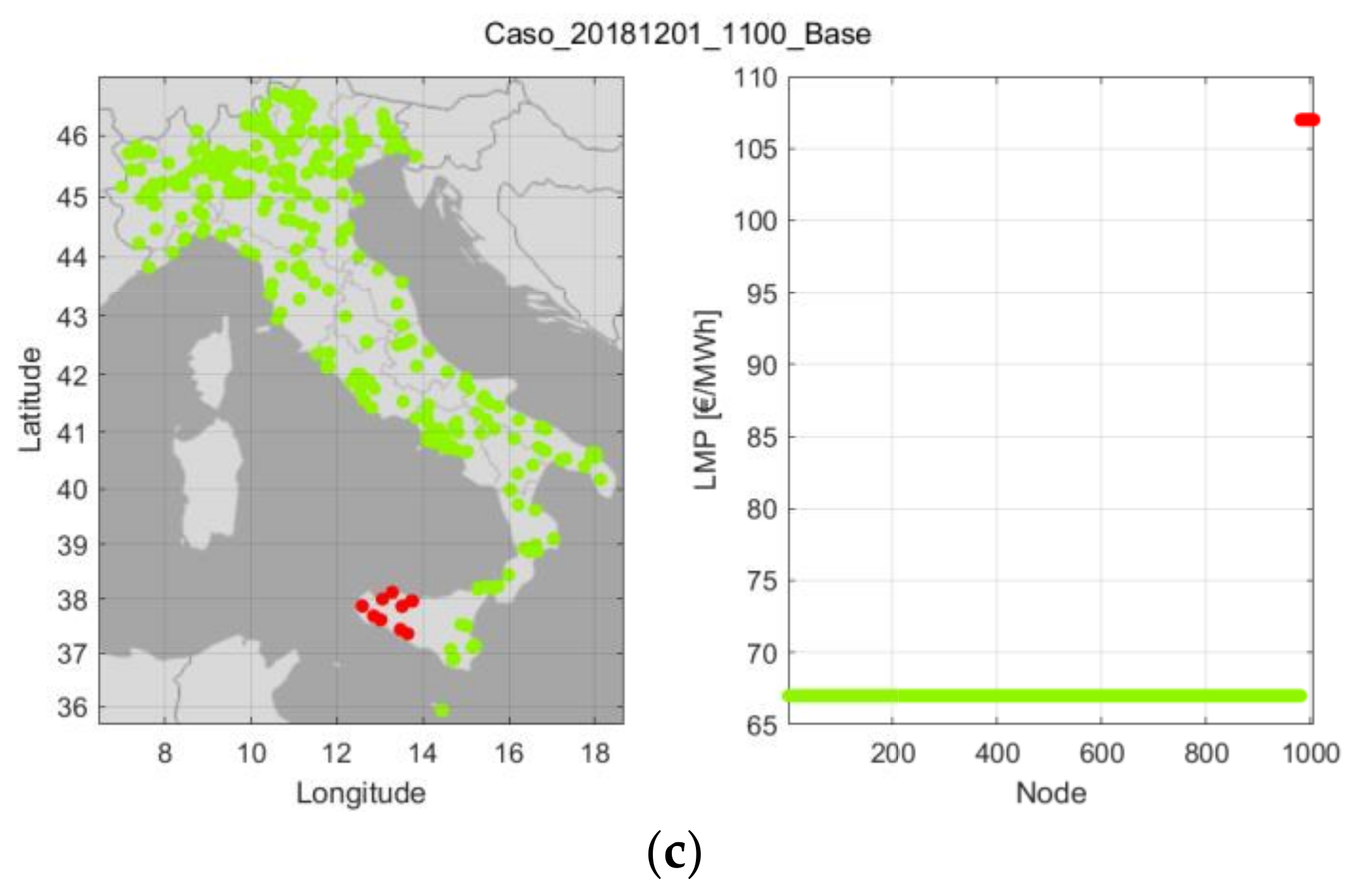
It should be mentioned that the work presented here is an extension of [29] where the basic algorithm is presented and it is shown that, for the Italian transmission system, the LMP patterns calculated by the algorithm (and, therefore, the corresponding congestions that determined them) for various snapshots of the 2018 Italian network data, present a correlation with the 2018 Italian market bidding zones configuration and that other known situation (like Italian NORD, or Sicily area inner congestions) can be detected. Therefore, the proposed approach can provide clustering algorithms with realistic data. Instead, the current work further develops the model by maturing (i) the identification procedure of critical contingencies, (ii) the solution for the management of the double line trips and (iii) the calculation of network indicators, including the PTDFs. However, the main contribution of the paper consists in extending the numerical analysis of the results: the entire range of considered snapshots (cases) and simulation scenarios (including comparison with the commonly encountered approach in literature when it comes to the calculation of network indicators for bidding zone configuration) is analyzed and the advantages of proposed approach are emphasized. Additionally, considerations about PTDFs as network indicators are also included. Moreover, a small network case was analyzed to prove the correctness of the proposed approach and the numerical performance of the proposed approach are shown.

Therefore, the goal of the current work is to develop a model for the calculation of network indicators to be used in a model-based definition of bidding zone configuration (first step of the process). The outputs of this work can be taken over by other works where the indicators here-calculated are processed by especially tailored clustering algorithms to identify alternative bidding zone configurations. For example, by paper [30] that considers only the LMPs, and by paper [31] which also considers the PTDFs.

2. Proposed Optimization Model

2.1. Optimization Problem Definition

A model-based methodology for alternative bidding zone configurations must be designed using computational models that include, among others: (i) a complete representation of the transmission network that considers explicitly all relevant security standards (contingency analysis, operational limits, etc.) and (ii) a detailed representation of the market rules (production costs, market bids, etc.). This requires the adoption of an advanced market model in which the electric grid is accurately represented: an optimal power flow (OPF) problem that integrates network security and market rules related constraints.

2.2. Objective Function and N Security Constraints

The generating units real power outputs are modeled using market bids defined according to the rules of the Italian day-ahead market [32] which allows the definition of up to three price–quantity pairs representing the economic bids for each production or consumption unit. Here, the proposed optimization problem is solved using historical data and thus the market clearing point is already available. Thus, for simplification, the demand is fixed to the quantity given by actual conditions. However, the model can be easily extended to consider variable demand using the same type of equations employed for the supply side and correctly considering the sign of the demand power. The goal of the optimization problem is the maximization the social welfare that, considering the demand is fixed, can be defined as the minimization of the total costs of generation acceptance:

$$\min \sum _{\begin{array}{c}k\in \mathcal{G}\\ m\in \mathcal{B}\end{array}} {\pi }_k^m · {\mathsf{\Omega }}_k^m$$

(1)

where $\mathcal{G}$ is the set of generating units; $\mathcal{B}$ is the set of supply bids; ${\pi }_k^m$ are the offered energy prices; ${\mathsf{\Omega }}_k^m$ are the accepted supply quantities for each m step of supply bid pertaining to kth generating unit. Variables ${\mathsf{\Omega }}_k^m$ are positive and upper bounded by the submitted quantities. The generators real power output is:

$$P_k=\sum _{m\in B}{\mathsf{\Omega }}_k^m, \forall k\in \mathcal{G}$$

(2)

Looking at Equation (2), it should be mentioned that the continuity of the generated power is guaranteed by the convexity requirements of the bids specified by the market rules [32] which paired with the minimization of (1) ensure the sequential acceptance, according to economic merit order, of the offered quantities.

The constraints of the optimization model are given by equations that model the transmission network operation constraints. The normal operating conditions are given by the DC PF model:

$$\mathit{P}={\mathit{B}}_{\mathit{b}\mathit{u}\mathit{s}}^{\mathit{N}} · {\mathit{\delta }}^{\mathit{N}}+{\mathit{B}}_{\mathit{P}\mathit{S}\mathit{T}}^{\mathit{N}} · {\mathit{\phi }}_{\mathit{P}\mathit{S}\mathit{T}}^{\mathit{N}}$$

(3)

where $\mathit{P}$ is the vector of real power injections into network buses calculated as the difference between the nodal generation and demand; ${\mathit{B}}_{\mathit{b}\mathit{u}\mathit{s}}^{\mathit{N}}$ is the bus admittance matrix of the DC PF method; ${\mathit{B}}_{\mathit{P}\mathit{S}\mathit{T}}^{\mathit{N}}$ is the bus to phase-shifting transformers (PST) admittance matrix; ${\mathit{\delta }}^{\mathit{N}}$ is the unknowns vector of the bus voltage angles (excluding the slack bus angle that is fixed to zero) and ${\mathit{\phi }}_{\mathit{P}\mathit{S}\mathit{T}}^{\mathit{N}}$ is the unknowns vector of PSTs angles. At this point, it should be noted that in order to distinguish between vector and scalar quantities, bold notation is used for the former.

The real power flows in the branches of the electric grid, ${\mathit{F}}^{\mathit{N}}$, are:

$${\mathit{F}}^{\mathit{N}}={\mathit{B}}_{\mathit{b}\mathit{r}}^{\mathit{N}} · {\mathit{\delta }}^{\mathit{N}}+{\mathit{B}}_{\mathit{b}\mathit{r}\mathit{P}\mathit{S}\mathit{T}}^{\mathit{N}} · {\mathit{\phi }}_{\mathit{P}\mathit{S}\mathit{T}}^{\mathit{N}}$$

(4)

where ${\mathit{B}}_{\mathit{b}\mathit{r}}^{\mathit{N}}$ and ${\mathit{B}}_{\mathit{b}\mathit{r}\mathit{P}\mathit{S}\mathit{T}}^{\mathit{N}}$ are the branch-to-nodes and branch-to-PSTs admittance matrices, respectively.

According to the N security criterion, these flows are limited in upwards and downwards directions by the maximum flow limits corresponding to the thermal limits of the network’s branches:

$$-{\mathit{F}}_{\mathit{m}\mathit{a}\mathit{x}}^{\mathit{N}}\le {\mathit{F}}^{\mathit{N}}\le {\mathit{F}}_{\mathit{m}\mathit{a}\mathit{x}}^{\mathit{N}}$$

(5)

where ${\mathit{F}}_{\mathit{m}\mathit{a}\mathit{x}}^{\mathit{N}}$ is the vector containing the maximum power flow allowed through the network’s branches, in general coinciding with the long-term thermal limit of the branch.

The generator’s and PST’s capability constraints are:

$${\mathit{P}}_{\mathit{G}}^{\mathit{m}\mathit{i}\mathit{n}}\le {\mathit{P}}_{\mathit{G}}\le {\mathit{P}}_{\mathit{G}}^{\mathit{m}\mathit{a}\mathit{x}}$$

(6)

$${\mathit{\phi }}_{\mathit{P}\mathit{S}\mathit{T}}^{\mathit{m}\mathit{i}\mathit{n}}\le {\mathit{\phi }}_{\mathit{P}\mathit{S}\mathit{T}}^{\mathit{N}}\le {\mathit{\phi }}_{\mathit{P}\mathit{S}\mathit{T}}^{\mathit{m}\mathit{a}\mathit{x}},$$

(7)

where ${\mathit{P}}_{\mathit{G}}$ is the vector containing the real power produced by all the generators in the grid, i.e., the vector containing $P_k$, $\forall k\in \mathcal{G}$; ${\mathit{P}}_{\mathit{G}}^{\mathit{m}\mathit{i}\mathit{n}}$ and ${\mathit{P}}_{\mathit{G}}^{\mathit{m}\mathit{a}\mathit{x}}$ are the vectors of lower and upper bounds for generator’s real powers production, respectively; ${\mathit{\phi }}_{\mathit{P}\mathit{S}\mathit{T}}^{\mathit{m}\mathit{i}\mathit{n}}$ and ${\mathit{\phi }}_{\mathit{P}\mathit{S}\mathit{T}}^{\mathit{m}\mathit{a}\mathit{x}}$ are the vectors of lower and upper bounds of the PST angles, respectively.

2.3. The N-1 Security–Preventive Criterion Constraints

The N-1 preventive security criterion assumes that following a network element outage (branch or generator) there is not enough time available to calculate and apply corrective actions that would solve potential resulting congestions; therefore, in these operating conditions the normal network operating constraints have to be satisfied.

2.3.1. Network Branch Outage

The impact of branch b outage on the real power flowing in branch a is evaluated using the Linear Outage Distribution Factors, i.e., $D{F}_a^b$, described by Enns et al. in [33]. Thus, the resulting N-1 preventive security constraints are given by:

$$-{\mathit{k}}_{\mathit{a},\mathit{b}}^{\mathit{p}\mathit{r}\mathit{e}\mathit{v}} · {\mathit{F}}_{\mathit{m}\mathit{a}\mathit{x},\mathit{a},\mathit{b}}^{\mathit{N}}\le {\mathit{F}}_{\mathit{a}}^{\mathit{N}}+\mathit{D}{\mathit{F}}_{\mathit{a}}^{\mathit{b}} · {\mathit{F}}_{\mathit{b}}^{\mathit{N}}\le {\mathit{k}}_{\mathit{a},\mathit{b}}^{\mathit{p}\mathit{r}\mathit{e}\mathit{v}} · {\mathit{F}}_{\mathit{m}\mathit{a}\mathit{x},\mathit{a},\mathit{b}}^{\mathit{N}}$$

(8)

Equation (8) is defined for all (a, b) pairs that are critical for the considered network. In Equation (8), ${\mathit{F}}_{\mathit{a}}^{\mathit{N}}$ and ${\mathit{F}}_{\mathit{b}}^{\mathit{N}}$ are unknown vectors of branches real power flows, i.e., elements of ${\mathit{F}}^{\mathit{N}}$, defined according to the considered set of (a, b) pairs: the nth element of ${\mathit{F}}_{\mathit{a}}^{\mathit{N}}$ and the nth element of ${\mathit{F}}_{\mathit{b}}^{\mathit{N}}$ represent the nth (a, b) pair. Parameter vector ${\mathit{F}}_{\mathit{m}\mathit{a}\mathit{x},\mathit{a},\mathit{b}}^{\mathit{N}}$ contains the maximum power flow limits of the critical branches a, while ${\mathit{k}}_{\mathit{a},\mathit{b}}^{\mathit{p}\mathit{r}\mathit{e}\mathit{v}}$ is a vector of user-defined coefficients to properly scale vector ${\mathit{F}}_{\mathit{m}\mathit{a}\mathit{x},\mathit{a}}^{\mathit{N}}$. If the preventive security criterion is adopted, then all elements of ${\mathit{k}}_{\mathit{a},\mathit{b}}^{\mathit{p}\mathit{r}\mathit{e}\mathit{v}}$ vector are equal to 1; if the corrective security criterion is adopted, then the elements of ${\mathit{k}}_{\mathit{a},\mathit{b}}^{\mathit{p}\mathit{r}\mathit{e}\mathit{v}}$ vector can be greater than 1 to allow temporary overload before corrective actions are applied, where the short-term thermal limits allow it, as will be explained in Section 2.4.

2.3.2. Generator Outage

The generation real power profile automatically changes at the outage of the kth generator due to the primary frequency regulation actions. Thus, for the mth generator participating in primary frequency regulation the variation of its real power output at the outage of the kth generator is:

$$\Delta P_m^k=\frac{e_m}{{\sum }_{jϵ\mathcal{G}}\left(e_j\right)} · P_k,$$

(9)

where $e_j$ is the regulating energy associated to primary frequency regulation of the $j$th generator. It is calculated as:

$$e_m=\frac{P_m^{max}}{R_m · f_n},$$

(10)

where $P_m^{max}$ is the maximum real power limit of mth generator (mth element of parameter vector ${\mathit{P}}_{\mathit{G}}^{\mathit{m}\mathit{a}\mathit{x}}$) in MW; $R_m$ is the statism of mth generator in p.u. while $f_n$ is the nominal frequency of the network in Hz.

Considering all generators, the real power change due to primary frequency regulation at the outage of kth generator is quantified by vector $\Delta {\mathit{P}}^{\mathit{f}\mathit{r}\mathit{e}\mathit{q},\mathit{k}}$ that includes all the $\Delta P_m^k$ elements, except for the slack generator which, according to the DC PF model, automatically adjusts its power variation. Finally, these power changes need not to violate generating units’ capability constraints:

$${\mathit{P}}_{\mathit{G}}^{\mathit{m}\mathit{i}\mathit{n}}\le {\mathit{P}}_{\mathit{G}}+\Delta {\mathit{P}}^{\mathit{f}\mathit{r}\mathit{e}\mathit{q},\mathit{k}}\le {\mathit{P}}_{\mathit{g}\mathit{G}}^{\mathit{m}\mathit{a}\mathit{x}},$$

(11)

The power flow in each branch considering the generation real power output following the outage of kth generator is determined by introducing the next constraints:

$$-{\mathit{k}}_{\mathit{a},\mathit{k}}^{\mathit{p}\mathit{r}\mathit{e}\mathit{v}} · {\mathit{F}}_{\mathit{m}\mathit{a}\mathit{x},\mathit{a},\mathit{k}}^{\mathit{N}}\le {\mathit{F}}_{\mathit{a}}^{\mathit{N}}+\Delta {\mathit{F}}_{\mathit{a}}^{\mathit{f}\mathit{r}\mathit{e}\mathit{q},\mathit{k}}\le {\mathit{k}}_{\mathit{a},\mathit{k}}^{\mathit{p}\mathit{r}\mathit{e}\mathit{v}} · {\mathit{F}}_{\mathit{m}\mathit{a}\mathit{x},\mathit{a},\mathit{k}}^{\mathit{N}},$$

(12)

where ${\mathit{k}}_{\mathit{a},\mathit{k}}^{\mathit{p}\mathit{r}\mathit{e}\mathit{v}}$ is a vector of user-defined coefficients to scale ${\mathit{F}}_{\mathit{m}\mathit{a}\mathit{x},\mathit{a},\mathit{k}}^{\mathit{N}}$ (same logic as with the previously defined ${\mathit{k}}_{\mathit{a},\mathit{b}}^{\mathit{p}\mathit{r}\mathit{e}\mathit{v}}$), while $\Delta {\mathit{F}}_{\mathit{a}}^{\mathit{f}\mathit{r}\mathit{e}\mathit{q},\mathit{k}}$ represents the variation of the power flow at branch a, linking node i to j, due to the outage of the kth generator:

$$\Delta {\mathit{F}}_{\mathit{a}}^{\mathit{f}\mathit{r}\mathit{e}\mathit{q},\mathit{k}}=\frac{{\mathit{X}}^{\mathit{i}}-{\mathit{X}}^{\mathit{j}}}{{\mathit{x}}_{\mathit{a}}} · \Delta {\mathit{P}}^{\mathit{f}\mathit{r}\mathit{e}\mathit{q},\mathit{k}},$$

(13)

where ${\mathit{X}}^{\mathit{i}, \mathit{j}}$ are the ith and jth rows of the inverse of ${\mathit{B}}_{\mathit{b}\mathit{u}\mathit{s}}^{\mathit{N}}$.

Equation (11) represents the capability limits of the remaining generators following the outage of the kth generator. Equation (12) limits the branch power flows following the outage of the kth generator to the defined limits. To limit the dimensions of the optimization problem, Equations (10) and (11) are considered only for the (a, k) pairs that are critical to the network, i.e., for the kth generators of which outages could congest branches a. Thus, the size of (11a) is equal to the number of outage generators, the size of (11b) and (12) is equal to the number of critical (a, k) pairs.

2.4. The N-1 Security-Corrective Criterion Constraints

According to the N-1 security-corrective criterion, in case of single line/generator outage, a current violation is allowed if it is within appropriate limits (typically 120% of the permanent thermal limit) and it is possible to identify and apply remedial actions (generation re-dispatch) within a short time (about 30 min) to mitigate the violation.

Figure 1 illustrates these operating conditions by showing the time evolution of the value of the current in a generic branch of the network considering the outage of another network element. As can be seen, satisfying the N-1 corrective security criterion involves three stages of time:

(i)

first, before the outage (N operating conditions), the maximum current limit for the considered generic branch is not reached—the network satisfies the N security criterion;

(ii)

an outage occurs and the current in the considered generic branch increases as a consequence but without violating the relaxed current limit (the short-term thermal limit)—the network satisfies a relaxed/equivalent N-1 preventive security criterion. The value of the current is contained enough to allow the operation of the considered generic branch for a short period of time, time necessary to determine the optimal corrective actions necessary to solve the congestion;

(iii)

the corrective actions are applied and the current in the considered generic line is again bellow its maximum—the congestion has been solved and the network now satisfies the N-1 corrective security criterion.

The three stages shown in Figure 1 need to be represented through adequate constraints in the considered optimization problem. The first stage is already modeled by constraints (5)–(7) which assure network security in N operating conditions. The second stage operating constraints is guaranteed by constraints (8)–(13) through a proper setting of the ${\mathit{k}}_{\mathit{a},\mathit{b}}^{\mathit{p}\mathit{r}\mathit{e}\mathit{v}}$ and ${\mathit{k}}_{\mathit{a},\mathit{k}}^{\mathit{p}\mathit{r}\mathit{e}\mathit{v}}$ parameters, i.e., to values that represent the short-term thermal limit of the branches. Therefore, only the calculation of the corrective actions and their effect (stage three) need to be mathematically formulated.

2.4.1. Network Branch Outage

The change in the power flow in branch a introduced by the application of corrective actions in case of outage of branch b, $\Delta F_a^b$, can be determined using sensitivities obtained from the DC PF model. Thus:

$$\Delta {\mathit{F}}_{\mathit{a}}^{\mathit{b}}=\mathit{D}{\mathit{F}}_{\mathit{G}}^{\mathit{b}} · \Delta {\mathit{P}}_{\mathit{G}}^{\mathit{b}} \forall \left(a,b\right),$$

(14)

where $\Delta {\mathit{F}}_{\mathit{a}}^{\mathit{b}}$ is the vector of $\Delta F_a^b$ variables for all the considered $\left(a,b\right)$ pairs; $\mathit{D}{\mathit{F}}_{\mathit{G}}^{\mathit{b}}$ is a sensitivity matrix expressing the variation of the flow in branch a at the variation of the generators real power profile, while $\Delta {\mathit{P}}_{\mathit{G}}^{\mathit{b}}$ is the vector of corrective redispatch actions of the generating units. Here, matrix $\mathit{D}{\mathit{F}}_{\mathit{G}}^{\mathit{b}}$ is obtained like the linear coefficients of Equation (13) with the difference that ${\mathit{X}}^{\mathit{i}, \mathit{j}}$ are now the ith and jth rows of the inverse of ${\mathit{B}}_{\mathit{b}\mathit{u}\mathit{s}}^{\mathit{N}-1,\mathit{a}}$, i.e., the bus admittance matrix obtained considering the outage of branch a.

Thus, the branch flows after the branch a outage and application of corrective actions, are constrained by:

$$-{\mathit{k}}_{\mathit{a},\mathit{b}}^{\mathit{c}\mathit{o}\mathit{r}} · {\mathit{F}}_{\mathit{m}\mathit{a}\mathit{x},\mathit{a},\mathit{b}}^{\mathit{N}}\le {\mathit{F}}_{\mathit{a}}^{\mathit{N}}+\mathit{D}{\mathit{F}}_{\mathit{a}}^{\mathit{b}} · {\mathit{F}}_{\mathit{b}}^{\mathit{N}}+\Delta {\mathit{F}}_{\mathit{a}}^{\mathit{b}}\le {\mathit{k}}_{\mathit{a},\mathit{b}}^{\mathit{c}\mathit{o}\mathit{r}} · {\mathit{F}}_{\mathit{m}\mathit{a}\mathit{x},\mathit{a},\mathit{b}}^{\mathit{N}} \forall \left(a,b\right),$$

(15)

where ${\mathit{k}}_{\mathit{a},\mathit{b}}^{\mathit{c}\mathit{o}\mathit{r}}$ is a user-defined vector of coefficients introduced in analogy with the other scaling coefficients, e.g., ${\mathit{k}}_{\mathit{a},\mathit{b}}^{\mathit{p}\mathit{r}\mathit{e}\mathit{v}}$, to scale ${\mathit{F}}_{\mathit{m}\mathit{a}\mathit{x},\mathit{a},\mathit{b}}^{\mathit{N}}$; if no particular requirements are in place, then all elements of ${\mathit{k}}_{\mathit{a},\mathit{b}}^{\mathit{c}\mathit{o}\mathit{r}}$ are 1, in agreement with what was explained previously. In Equation (15) the equivalent preventive and corrective steps of the N-1 security-corrective criterion (second and third stages in Figure 1) are in superposition: this is allowed by the linearity of the DC PF model. The corrective actions need to comply with the generator’s capabilities:

$${\mathit{P}}_{\mathit{G}}^{\mathit{m}\mathit{i}\mathit{n}}\le {\mathit{P}}_{\mathit{G}}+\Delta {\mathit{P}}_{\mathit{G}}^{\mathit{b}}\le {\mathit{P}}_{\mathit{G}}^{\mathit{m}\mathit{a}\mathit{x}} \forall \left(b\right),$$

(16a)

$$\Delta {\mathit{P}}_{\mathit{G}}^{\mathit{d}\mathit{w}} \le \Delta {\mathit{P}}_{\mathit{G}}^{\mathit{b}}\le \Delta {\mathit{P}}_{\mathit{G}}^{\mathit{u}\mathit{p}} \forall \left(b\right),$$

(16b)

where $\Delta {\mathit{P}}_{\mathit{G}}^{\mathit{d}\mathit{w}}$ and $\Delta {\mathit{P}}_{\mathit{G}}^{\mathit{u}\mathit{p}}$ are vectors quantifying the ramp-up and -down generator limits, respectively.

2.4.2. Generator Outage

As with the case of branch outage, the case of generator outage is also necessary to model the corrective actions and their impact on the branches’ power flow. The variation of the power flow in branch a at the application of the corrective actions following the outage of generator k,$\Delta F_a^k$, is quantified using the same approach as in (14):

$$\Delta {\mathit{F}}_{\mathit{a}}^{\mathit{k}}=\mathit{D}{\mathit{F}}_{\mathit{G}}^{\mathit{k}} · \Delta {\mathit{P}}_{\mathit{G}}^{\mathit{k}} \forall \left(a,k\right),$$

(17)

where $\Delta {\mathit{F}}_{\mathit{a}}^{\mathit{k}}$ is the vector of $\Delta F_a^k$ variables for all the considered $\left(a,k\right)$ pairs; $\mathit{D}{\mathit{F}}_{\mathit{G}}^{\mathit{k}}$ is a sensitivity matrix that expresses the variation of the flow in branch a at the variation of the generators real power profile, while $\Delta {\mathit{P}}_{\mathit{G}}^{\mathit{k}}$ is the vector of corrective redispatch actions of the generating units. Matrix $\mathit{D}{\mathit{F}}_{\mathit{G}}^{\mathit{k}}$ is obtained as the linear coefficients of Equation (12) and, since the network topology does not vary when generator outages occur, then it remains invariant no matter the outage.

Thus, the branch flow constraints following the outage of generator k and the application of the corrective actions, for all the considered $\left(a,k\right)$ pairs, are given by the following equation:

$$-{\mathit{k}}_{\mathit{a},\mathit{k}}^{\mathit{c}\mathit{o}\mathit{r}} · {\mathit{F}}_{\mathit{m}\mathit{a}\mathit{x},\mathit{a},\mathit{k}}^{\mathit{N}}\le {\mathit{F}}_{\mathit{a}}^{\mathit{N}}+\Delta {\mathit{F}}_{\mathit{a}}^{\mathit{f}\mathit{r}\mathit{e}\mathit{q},\mathit{k}}+\Delta {\mathit{F}}_{\mathit{a}}^{\mathit{k}}\le {\mathit{k}}_{\mathit{a},\mathit{k}}^{\mathit{c}\mathit{o}\mathit{r}} · {\mathit{F}}_{\mathit{m}\mathit{a}\mathit{x},\mathit{a},\mathit{k}}^{\mathit{N}} \forall \left(a,k\right),$$

(18)

where ${\mathit{k}}_{\mathit{a},\mathit{k}}^{\mathit{c}\mathit{o}\mathit{r}}$ is a user-defined vector of coefficients introduced in analogy with the other scaling coefficients, e.g., ${\mathit{k}}_{\mathit{a},\mathit{b}}^{\mathit{p}\mathit{r}\mathit{e}\mathit{v}}$, to scale ${\mathit{F}}_{\mathit{m}\mathit{a}\mathit{x},\mathit{a}}^{\mathit{N}}$; if no particular requirements are in place, then all elements of ${\mathit{k}}_{\mathit{a},\mathit{k}}^{\mathit{c}\mathit{o}\mathit{r}}$ are 1, in agreement with what was explained in previous section. In Equation (17), similarly to Equation (14), the equivalent preventive and corrective steps of the N-1 security-corrective criterion are in superposition. The corrective actions need to be also constrained by the generators’ capabilities:

$${\mathit{P}}_{\mathit{G}}^{\mathit{m}\mathit{i}\mathit{n}}\le {\mathit{P}}_{\mathit{G}}+\Delta {\mathit{P}}^{\mathit{f}\mathit{r}\mathit{e}\mathit{q},\mathit{k}}+\Delta {\mathit{P}}_{\mathit{G}}^{\mathit{k}}\le {\mathit{P}}_{\mathit{G}}^{\mathit{m}\mathit{a}\mathit{x}} \forall \left(k\right),$$

(19a)

$$\Delta {\mathit{P}}_{\mathit{G}}^{\mathit{d}\mathit{w}}\le \Delta {\mathit{P}}_{\mathit{G}}^{\mathit{k}}\le \Delta {\mathit{P}}_{\mathit{G}}^{\mathit{u}\mathit{p}} \forall \left(k\right),$$

(19b)

2.5. Constraints on Critical Sections

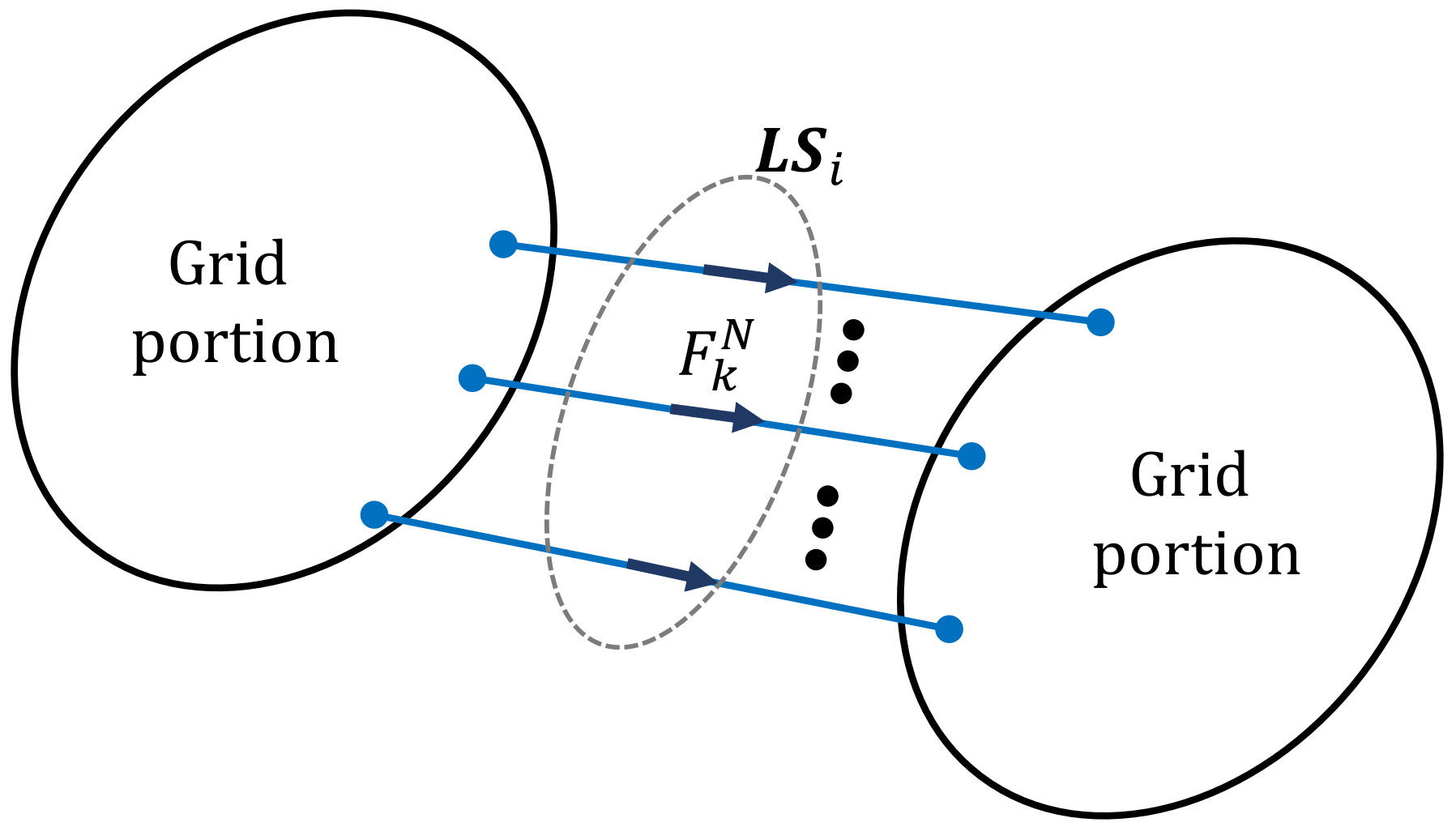
In actual network operation it is possible that some portions of the grid are weakly meshed or there is a scarcity of control resources available and, as consequence, high power (current) flows through some sections of the grid introducing high voltage drops that are difficult to manage. For these cases, the DC PF model is not able to directly assess the potential voltage problems: maximum flow constraints on some network interfaces (set of network branches connecting various portions of the electric grid) are introduced:

$$F_i^{min}\le {\sum }_{k\in \mathit{L}{\mathit{S}}_i}{F}_k^N\le F_i^{max}\forall \mathit{L}{\mathit{S}}_i\subseteq \mathit{C}\mathit{S},$$

(20)

where $\mathit{L}{\mathit{S}}_i$ is the set of branches included in the critical section i (see Figure 2); $\mathit{C}\mathit{S}$ is the set of critical sections, with $\mathit{L}{\mathit{S}}_i\in \mathit{C}\mathit{S}$; $F_i^{max}$ and $F_i^{min}$ are the maximum and minimum power flow limits on the critical section i, respectively; they can be obtained from off-line network studies.

2.6. Definition of the Critical Branches–Critical Outages Sets

The defined DC OPF problem is characterized by a high sparsity index as it relies on a complete approach, unlike the compact models: the equations that guarantee the power balance of the system represent the entire set of power flow equations. Compared to compact models, this defined model uses a much larger number of variables and equations, but, at the same time, due to its sparsity can easily be solved by linear, large-scale, optimization solvers. However, this does not mean that it is not important to contain, as much as possible, the size of the optimization problem (the number of variables and number of constraints): the smaller it becomes, the faster it is solved. A key role in the proposed optimization problem is played by the equations modelling the security criteria: without any intervention there should be (i) as many equation sets as there are branches in the network for N security conditions and, (ii) as many (a, b) and (a, k) pairs as the network topology and number of generators allows for N-1 security conditions. This, for a real network, would result in an extremely large number of variables and constraints, impossible to be dealt with even by the best performing optimization solvers. Therefore, it is necessary to minimize the set of branches constrained in N security conditions and for the (a, b) and (a, k) pairs to be constrained in N-1 security conditions. The following iterative procedure consisting in the sequential update of the set and finding the solution to the DC OPF problem, is adopted:

Step 0 

consider an initial generation real power production profile and set the iteration counter to iter = 1; consider the set of critical branches in N security conditions, i.e., the set used to formulate constraints (5), null; consider the set of critical (a, b) and (a, k) pairs, i.e., the sets used to formulate the constraints of the DC OPF model, null;

Step 1 

calculate $D{F}_a^b$ sensitivities and the constant coefficient terms of Equation (11) for all the (a, b) and (a, k) pairs. Since the DC PF model is sparse and linear this calculation is very fast;

Step 2 

compute the DC PF solution using the generation real power production profile at iteration iter in N operating conditions;

Step 3 

Update the set of critical branches in N security conditions by adding the new branches for which:

$$\left|{\mathit{F}}^{\mathit{N}}\right|\ge e_1 · {\mathit{F}}_{\mathit{m}\mathit{a}\mathit{x}}^{\mathit{N}},$$

(21)

while keeping the already present branches in the set.

In Equation (21) $e_1$ is a user-defined parameter; for this paper, its value has been set to 0.7, a value that allows a reduced number of iterations without losing any critical branches from inclusion in the set.

Step 4 

Update the set of critical (a, b) pairs by adding the new branches for which:

$$F_a^N+D{F}_a^b · F_b^N\ge e_2 · F_{max,a}^N,$$

(22a)

$$D{F}_a^b · F_b^N\ge e_3 · F_{max,a}^N,$$

(22b)

with $e_2$ and $e_3$ being user-defined parameters.

Basically, a pair (a, b) should be included in the optimization problem if the outage of b brings the power flow in branch a above a critical threshold quantified by parameter $e_2$ in Equation (22a), with $e_2$ being lower than 1. However, this can be too constrained for low values of $e_2$ where there is the risk of including branches with low values of initial power flow that see small variations in their power flow due to outage of b, therefore are not actually critical. Alternatively, it can be too relaxed for high values of $e_2$ where there is the risk to omit branches that see a large variation in their power flow due to outage of b but don’t violate the high values of $e_2$, therefore branches that are actually critical. To mitigate these flaws condition (22b) is also introduced: if the threshold given by $e_3$ is reached then it means that outage of b has significant impact on power flow in branch a. After extensive preliminary studies, it was found that three pairs of ($e_2$, $e_3$) values are sufficient to detect all critical (a, b) pairs: ($e_2$, $e_3$) = {(0.2, 0.7), (0.1, 0.9), (0.01, 0.99)}. If an (a, b) pair satisfies (22) for at least one ($e_2$, $e_3$) pair of values, then it should be included in the optimization problem. Clearly, the last pair value, i.e., (0.01, 0.99) is the most conservative and it should detect, by itself, all critical (a, b) pairs or, in other words, all congested branches a following the outage of branches b. However, the optimal solution changes with the update of the (a, b) set and there is the risk of performing too many iterations due to previously not detected (a, b) pairs. To mitigate this, the set of (a, b) pairs is broadened by also adopting softer values for ($e_2$, $e_3$) values.

As in the previous step, the already present (a, b) pairs are maintained in the set;

Step 5 

Update the set of critical (a, k) pairs by adding the new branches for which:

$$\Delta F_a^{freq,k}\ge e_2 · F_{max,a}^N,$$

(23a)

$$F_a^N+\Delta F_a^{freq,k}\ge e_3 · F_{max,a}^N,$$

(23b)

Basically, a pair (a, k) is included in the optimization problem if the outage of k has significant impact on a, (23a) and if it brings the power flow in a into a critical region, (23b). As in the previous step, the already present (a, k) pairs are maintained in the set;

Step 6 

If the sets of critical branches in N security conditions and the sets of critical (a, b) and (a, k) pairs at iteration iter are the same as in the previous iteration, iter-1, then STOP.

Step 7 

find the DC OPF solution; update the iteration index iter = iter + 1 and go to Step 2.

2.7. Calculation of Network Indicators

Starting from the results of the OPF, the electric grid indicators related to optimal electricity market clearing can be calculated and employed by clustering algorithms to propose alternative bidding zones configurations. Taking into account [10,11], two different indicators are considered: the locational marginal prices (LMPs) and the power transfer distribution factors (PTDFs).

The LMPs are the nodal marginal electricity prices and are calculated, in general, using the Lagrange multipliers of the constraints of the OPF problem. In this paper, the LMPs are computed starting from the solution provided by the proposed DC OPF model where the security criteria are modelled explicitly. In this way, the LMPs reflect the adopted hypotheses and therefore reflect both the technical requirements of power system operation and the energy market efficiency requirements and its rules. In particular, they are equal to the Lagrangian multipliers of the power flow equations in normal operating conditions (3): these constraints quantify the nodal power balance and, therefore, the Lagrangian multipliers of these constraints quantify the variation of the objective function (total cost of generation) at a change of a parameter in these equations (e.g., nodal demand variation), therefore they represent the nodal marginal price of energy according to the market clearing solution. Moreover, Equation (3) determines the vectors of independent variables ${\mathit{\delta }}^{\mathit{N}}$, which, in turn, determine the power flows through the branches ${\mathit{F}}^{\mathit{N}}$. The latter variables are subject also to the N-1 security criteria constraints of the model and, therefore, the LMPs values are implicitly influenced by the security related constraints when they are activated.

In general, the PTDFs are defined as the sensitivity of the power flow variation in a branch of the network at the variation of a bus power injection [10]. To calculate the PTDF of a generic branch k connecting bus i to bus j one needs to first consider the expressions of the power flows in the branch. For the DC PF model, only the real power flow in the branch, $F_k^N$, can be calculated as:

$$F_k^N=\frac{{\delta }_i-{\delta }_j}{x_k}$$

(24)

where $x_k$ is the reactance of branch k.

According to the DC PF model (3) and in the absence of the PST angles, the vector of voltage angles $\mathit{\delta }$ can be expressed as:

$$\mathit{\delta }=\mathit{X} · \mathit{P}$$

(25)

where $\mathit{X}$ is the inverse of ${\mathit{B}}_{\mathit{b}\mathit{u}\mathit{s}}^{\mathit{N}}$.

Thus, (24) becomes:

$$F_k^N=\frac{{\mathit{X}}^{\mathit{i}}-{\mathit{X}}^{\mathit{j}}}{x_k} · \mathit{P}$$

(26)

Now, (26) includes the nodal power injections in vector $\mathit{P}$. Therefore, the variation of the flow in branch k at the variation of the nodal power injection at bus p, i.e., the PTDF of branch k at the variation of the nodal power at bus p, can be calculated as:

$$PTD{F}_k^p=\frac{\partial F_k^N}{\partial P_k}=\frac{X_{ip}-X_{jp}}{x_k}$$

(27)

where $X_{ip}$ and $X_{jp}$ are the ip and jp elements of matrix $\mathit{X}$, respectively.

Looking at (27) it is now clear why the PST angles have been neglected from the beginning: if considered, according to (3) the same results of (27) would have been obtained since the flow $F_k^N$ of (26) would have resulted in a linear combination between nodal power injections and the PST angles and therefore, the derivative $\frac{\partial \left(·\right)}{\partial P_k}$ would have resulted null for the PST angles terms, in any case.

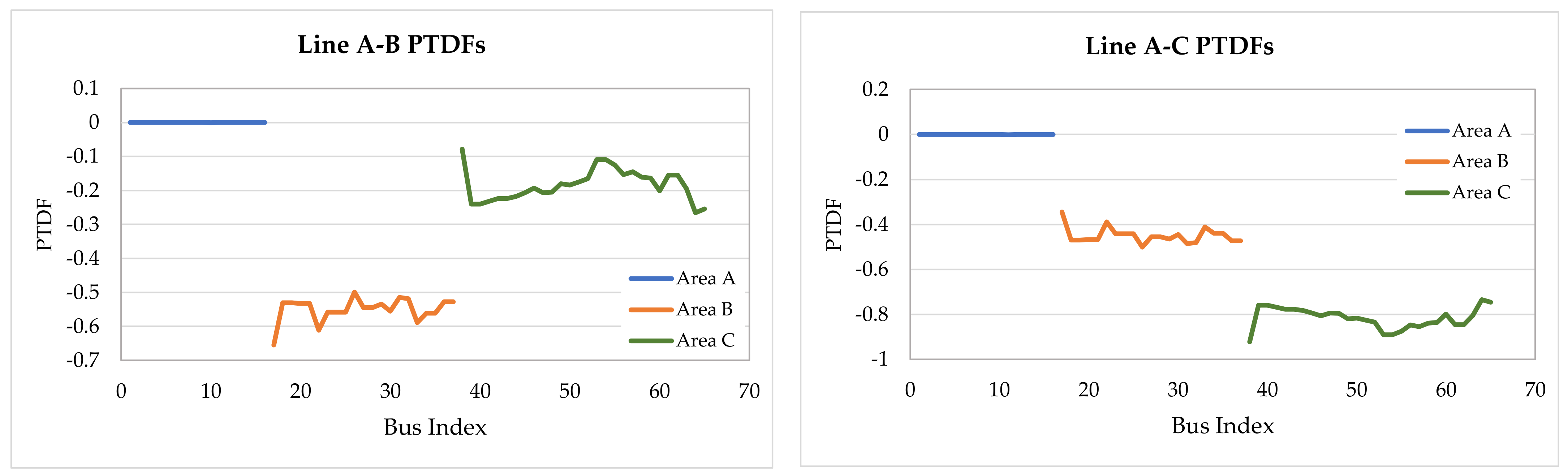
It is interesting to note that (27) is invariant with respect to the network operating conditions (the values of $\mathit{\delta }$, $\mathit{P}$, ${\mathit{\phi }}_{\mathit{P}\mathit{S}\mathit{T}}$) but it depends strictly on the network topology and parameters. In these conditions the PTDFs do not depend on the results of the proposed optimization problem therefore, they could be calculated for the entire grid. However, the solution of the proposed optimization problem is very important because besides providing the LMPs, it also provides the set of congested lines (i.e., the set of branches for which the flow bounds are activated either in N or N-1 security conditions): the PTDFs of the identified congested branches can therefore be extracted and used as network indicators to provide the clustering algorithms with important topological data. In details, for a given congested branch, the buses with similar PTDFs are the buses that can influence similarly the power flow in the congested branch and therefore, if topologically coherent, could form a bidding zone, or constitute part of a bigger one. Paper [31] explains in detail how the PTDFs can be used for the definition of bidding zones.

2.8. Strategies to Enforce the Robustness of the Optimization Problem

In general, if the DC OPF problem is infeasible and a solution cannot be found, then the iterative procedure defined in the previous subsection halts without the satisfaction of the stopping criterion. Various numerical tests have shown this situation to occur when a branch outage leaves a portion of the grid in radial configuration characterized only by demand buses, as shown in Figure 3. In this situation, the demand may require more power than the limits of the radially connected branches allow and, since the demand is not controllable by the optimization, the DC OPF model will diverge due to the impossibility of satisfying constraints (8). This situation is a consequence of a simplified network model adopted that does not represent the 150 kV grid (it includes the 380/220 kV grid) which, in case of occurrence of the considered outage would be able to supply the demand, and/or of the DC PF model simplifying hypothesis, in particular the fact that the nodal voltage magnitude is considered equal to 1 p.u.; if the AC PF model were adopted, a lower nodal voltage profile would determine lower currents and, hence, the possibility to satisfy the branch current constraints.

To mitigate this situation, a pair of fictitious generators are considered at specific buses in the grid: one that can produce between −1000 MW and 0 MW and offered at a very low and negative price, and another that can produce between 0 MW and +1000 MW and offered at a very high positive price. These prices have been set at −3000 €/MWh, and +3000 €/MWh (the cap limit of the Italian market bids [32]), respectively. Moreover, these generators are dispatched only to provide corrective actions and therefore, for them, $P_k=0$, $\Delta P_G^b$ is dispatchable and penalized by the fictious prices in the objective function. Thus, since they have very high prices, they are characterized by the lowest dispatch priority among all generators and, thus, they will be accepted only if necessary, i.e., to satisfy the N-1 security constraints.

2.9. Modelling of Multiple Line Outages

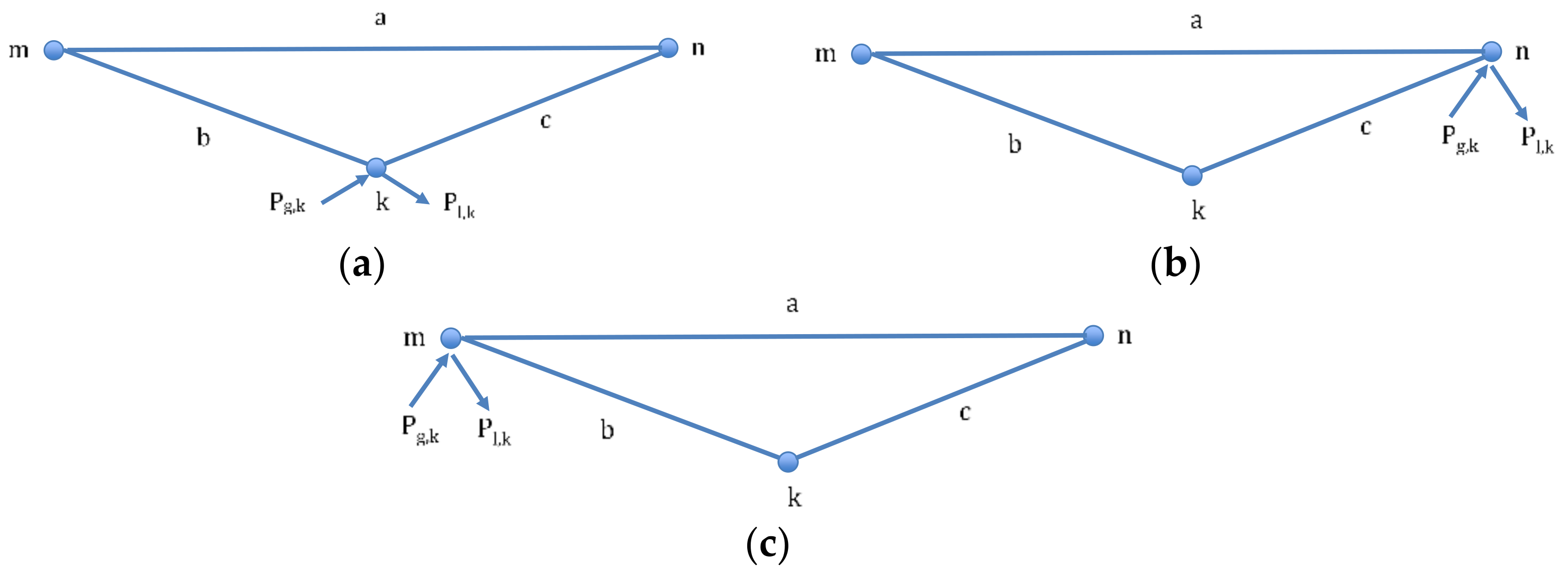
Some network operating conditions involve the simultaneous loss of two or more transmission branches. This is the case of electric lines that share, partially or fully, the same sustaining pillars: an outage due to damage at a sustaining pillar will outage all the involved electric lines. In general, there are no more than two electric lines involved, therefore this case is going to be further considered. In the case the share of sustaining pillars is full then the two lines are perfectly connected in parallel: the double outage is immediately implemented by modifying the network model and replacing the double lines with a single connection consisting of the parallel of the two.

In case of partial share of sustaining pillars, the situation is more complex because one of the ends of the two lines is not the same. These situations are illustrated in Figure 4 where the double outage is made of either outage (a, b) or (a, c). This situation is managed by adapting the network model and moving the electrical demand and generation production present at bus k into buses n or m depending on whether the double outage regards branches (a, b) or branches (a, c), as illustrated in Figure 4a,b, respectively. For both cases, this allows to consider the equivalent branch made of the parallel of a with the series of b + c and then simulate the double outage as the outage of the equivalent branch. It should be noted that this approach is able to model the effects of the double line trip only for the part of the grid outside ring (a, b, c). However, the approximation is found reasonable since the actual double line trip leaves bus k radially connected to the external grid and the nodal power of bus k is, in general, contained.

3. Numerical Tests

The proposed optimization model is a linear programming (LP) problem and, thus, it was implemented in GAMS environment [34] and CPLEX solver was deployed to find the solution. To guarantee the best feasible solution point, the optimality tolerance was set to 1 × 10⁻⁶ which, when related to the scale of the objective function, means 1 × 10⁻⁶ €, while the expected objective function value is of order at least equal to 1 × 10⁴ €. For all the performed simulations here described, the convergence criteria adopted by CPLEX to stop the algorithm were always completely fulfilled, meaning the mathematically optimal solution of the optimization problem has always been found. The procedure from Section 2.6 and all the data elaboration processes were developed in MATLAB [35]. The GAMS-MATLAB interaction was achieved through MATLAB scripts. All scenarios have been solved with a desktop PC equipped with an Intel(R) Core(TM) i7-7700HQ CPU @ 2.80 GHz 2.80 GHz processor and 16 Gb RAM.

3.1. The PST 16-Machine Test System

First, a simple test system is here shown to outline the main characteristics of the algorithm. The PST 16-machine test system [36] contains three different generator units, such as hydropower, thermal and nuclear. The rated power of these units is 220 MW, 247 MW and 259 MW, respectively. The power plants consist of a particular number of similar units connected to the network as can be seen in Figure 5: from G1 to G16. The system consists of three strongly meshed areas: Areas A, B and C, respectively, and each has 5–6 generators. Three long transmission lines connect these areas: A-C, A-B and B-C. The system is designed for power exchange between these areas. Area A contains mostly hydro power plants and is a power exporting area. Areas B and C are load demanding areas that import power from Area A. For this paper, the spring operating conditions [37] have been selected while the network parameters are obtainable from [38]. Finally, for simplicity, the generator bids have been assumed consisting of only one step covering the entire capability of the generating units and random prices have been assigned to them such that they qualitatively correspond to the technology marginal price and such that the unconstrained market solution will replicate the network characteristics: Area A exporting to Areas B and C.

Table 1. Generator bids for the PST 16-machine test system.

Generator	Area	Price [€/MWH]
G1	Area A	53
G2	Area A	63
G3	Area A	18
G4	Area A	24
G5	Area A	31
G6	Area A	40
G7	Area B	79
G8	Area B	96
G9	Area B	35
G10	Area B	86
G11	Area B	73
G12	Area C	82
G13	Area C	76
G14	Area C	97
G15	Area C	18
G16	Area C	22

shows these prices: Area A generators (hydro) present the smallest prices.

For illustrative purposes only the inter-area lines, i.e., A-B, A-C and B-C will be considered with the power flow limited by N and/or N-1 security criteria, and only the outages of these three lines will be considered. In this case, it is worth mentioning that the linear outage distribution factor, $D{F}_a^b$, for lines A-B and A-C = 1, meaning that in case of outage of one of the two the other will receive its entire N operating conditions flow. Three types of simulation scenarios have been considered: (i) the N100 scenario, where only the N security conditions have been considered and the long-term thermal limit of the inter-area lines have been applied; (ii) the N1prev scenario, where the N-1 preventive security criterion has been adopted and the long-term thermal limits of the inter-area lines have been applied for both N and N-1 operating conditions, and (iii) the N1cor scenario, where the N-1 corrective security criterion has been adopted and the long-term thermal limits have been applied for the N and N-1 post-corrective-actions operating conditions, while the short-term thermal limit (120% of the long-term one) has been considered for the N-1 pre-corrective-actions operating conditions.

Figure 6 shows the results in terms of accepted quantity of all generators scaled to their maximum capability for all the considered scenarios.

Table 2. Power flows on inter-area lines for N100 scenario.

Branch	FN [MW]	FNmax [MW]
A-B	1480.51	2300
A-C	2233.50	2300
B-C	−356.41	2530

shows the power flows on the inter-area lines for the N100 scenario: Area A exports to the other two areas, no inter-area line is congested, all the generators of Area A are accepted while the marginal generator is G7 of Area B; moreover, according to Figure 6, all generators that offered at a price higher than G7 have been fully rejected and all generators that offered at a price lower than G7 have been fully rejected. Clearly, this solution corresponds to the ideal market solution: indeed, no congestion has been activated and all the LMPs are equal to the price of G7, i.e., 79 €/MWh. Since the LMPs are all equal as no congestion is activated, this snapshot of the network operating conditions would suggest one bidding zone, i.e., the entire grid.

However, Table 2 shows that for outage of line A-B or A-C the other line transferring power from Area A would heavily congest: remembering that $D{F}_a^b=1$ for these two lines, the outage of line A-B would give a flow of about 3700 MW on line A-C; with the same effect for the outage of line A-C on line A-B. Therefore, the N100 scenario solution is not N-1 secure.

Figure 7 shows the power flows in lines A-B and A-C for all the stages of the adopted N-1 security criteria as calculated by the constraints of the optimization problem for the N1prev and N1cor scenarios. In both cases contingencies occur following the outages: the long-term limit is reached in N1prev scenario while the short-term limit is reached in N1cor scenario, which is then brought back to the long-term limit following the corrective actions. Clearly, since the short-term limit is higher than the long-term limit the flows in normal operating conditions are higher for the N1cor scenario than for the N1prev scenario: the inter-area lines are better exploited in the N1cor scenario as the flows are higher. However, when compared to the values of Table 1 the flows are lower in both cases.

This has an impact on the dispatch of the generators: the cheaper generation of Area A can no longer be fully accessed by the demand of Areas B and C: according to Figure 6, not all generators of Area A are now accepted and more expensive generators with respect to N100 scenario are now accepted in Areas B and C. The LMPs reflect this situation: in both N1prev and N1cor scenarios the LMPs of the buses of Area A are different from the LMPs of the buses of Areas B and C: (i) for N1prev scenario the LMPs of Area A are 53 €/MWh while the LMPs of Areas B and C are 86 €/MWh; (ii) for N1cor scenario the LMPs of Area A are 63 €/MWh while the LMPs of Areas B and C are 82 €/MWh. These values correspond to the prices offered by the partially accepted generators in both scenarios (see Figure 6 and Table 1), which is in complete agreement with the economic theory. To conclude, for this snapshot of the network operating conditions, we have congestions activated and the LMPs are distinguishable into two groups: two bidding zones separated by congested lines can be identified: Area A, on one side, and Areas B and C on the other side.

Figure 8 shows the PTDFs calculated for the two lines suggested by the optimization problem, A-B and A-C, calculated using Equation (27) and, therefore, invariant to the network operating conditions, but topologically dependent. As one can see, the buses with coherent PTDFs can be grouped in the three described areas. To be noted that the PTDFs of Area A are about 0; this is a consequence of having the slack bus present in Area A: any change in the nodal power at a bus of Area A will be compensated by the variation of the slack bus power and the power exchanged between the two will occur within Area A. For this snapshot of the network operating conditions the calculated LMPs are coherent with the areas identified by the PTDFs so, now, the PTDFs just confirm the LMP results. However, this may not always be the case: internal area congestions may lead to a disperse LMP profile within the areas, a profile that may lead the clustering algorithm to identify many small bidding zones, which is not advantageous from a market efficiency point of view. In this case, the information quantified by the PTDFs can help to identify more consistent bidding zones.

Of course, here punctual information has been commented while a bidding zones identification process implies that the network indicators obtained for a large set of possible network operating conditions are properly clustered by especially designed clustering algorithms that can identify coherent patterns within the data, that is not part of the present work (for this see, for example, [30,31]). What is important here is that the proposed algorithm gives market indicators coherent to the network operating conditions, adopted security criterion and market rules.

3.2. Italian Transmisssion Network Analysis

3.2.1. Test Cases Identification

The proposed optimization model is here tested on various electric grid models representing specific operating conditions of the Italian transmission grid identified by the TSO. A set of base cases representing specific hours of the year 2018 (

Table 3. Selected 2018 base cases.

DATETIME	HYDRO [MW]	SOLAR [MW]	WIND [MW]	IMPORT [MW]	DEMAND [MW]
01 February 2018 01:00	1500	0	2400	5700	26,700
14 February 2018 15:00	3400	3700	2700	7100	45,100
24 February 2018 01:00	2300	0	4500	5400	27,200
5 March 2018 03:00	2000	0	2100	5300	22,700
15 March 2018 22:00	3500	0	4100	6000	34,900
24 April 2018 09:00	8900	5500	400	3800	39,400
30 April 2018 00:00	6700	0	1200	3000	23,000
6 May 2018 10:00	7400	5900	1400	800	26,400
14 June 2018 06:00	7800	300	1100	5000	31,000
6 July 2018 07:00	7200	1700	2400	5800	39,000
16 July 2018 06:00	4900	200	800	5500	31,000
17 July 2018 12:00	5000	8700	2300	5100	44,900
10 September 2018 17:00	6900	3000	900	3800	42,700
23 October 2018 20:00	4300	0	3600	6200	40,000
24 October 2018 11:00	2600	8100	1300	5700	40,600
1 November 2018 04:00	4200	0	2300	2400	22,400
3 November 2018 07:00	5100	200	1400	5700	26,200
1 December 2018 11:00	4600	3000	600	4400	35,500
8 December 2018 10:00	3400	4100	5300	4000	30,900
31 December 2018 08:00	4500	1000	3000	2300	28,500

) have been selected by applying an “unsupervised learning” (k-means) classification algorithm on the hourly operating scenarios recorded in 2018.

Each hourly scenario is described by the following relevant quantities for the macro zones North + Center North, Center South + South, Sicily, and Sardinia [32]:

• Electricity demand,
• Hydropower production,
• Photovoltaic production,
• Wind production,
• Import from neighboring countries.

The number of clusters has been set to twenty so as to have the best compromise between the limitation of the quantity of processed data and intra-cluster variance minimization. For each cluster, the hourly scenario nearest to the centroid according to Euclidean distance, was selected as the base case. Thus, twenty base cases have been identified and, for each of them, four topological variants have been generated by considering a pre-selected 380 kV line in maintenance, one at a time. Figure 9 shows the pre-selected lines corresponding to these variants. In total, the proposed optimization problem was run on 100 cases (each of the 20 base cases has been simulated without outages and in the 4 variants).

Additionally, the border between the actual Central North (CN) and Central South (CS) bidding zones (according to the Bidding Zone configuration in place in 2018) has been represented as a relevant critical section according to (19) (see Figure 9).

For each base case and for each related variant, the offers accessible in the public offers corresponding to the time and day of the related base case, as published on the website of the Italian power exchange, GME [40] have been used. For each of them, the model is carried out assuming the N-1 security-corrective criterion. Therefore, both the N-1 security (equivalent) preventive and corrective related constraints are considered. Theoretically, the set of possible line outages consists of all 220 kV and 400 kV transmission lines and 220/400 kV transformers. Moreover, the set of the generators is made of all the generators included in the network model. In practice, the sets are built dynamically adopting the procedure described in Section 2.6.

Finally, the interconnection with the foreign countries and with the HV sub-transmission network (nominal voltages bellow 220 kV) are represented in the grid model using fixed injections (positive or negative) at the first bus located in the foreign country and at the HV side of the EHV/HV transformer, respectively.

3.2.2. Results

To evaluate the impact the proposed model has on the network operation and indicators for bidding zones configuration, simulations were performed in three scenarios:

(i)

N1cor—where the N-1 corrective security criterion (see Section 2.4 for details) is adopted and the full optimization model is deployed;

(ii)

N1prev—where the N-1 preventive security criterion is adopted;

(iii)

N70—where no explicit N-1 security criterion is considered but the most common strategy adopted in the literature related to alternative bidding zone configuration definition [17,18,19] is employed: only N security criterion is adopted and the maximum limit on the transmission branches power flow is lowered to 70% of the thermal limit, which is the most conservative value encountered.

From a modelling perspective, scenario N1cor considers all constraints proposed and relaxes the limits of the branches’ flows in the equivalent N-1 preventive security stage (see Figure 1) to 120% the thermal limit, i.e., coefficients ${\mathit{k}}_{\mathit{a},\mathit{b}}^{\mathit{p}\mathit{r}\mathit{e}\mathit{v}}$ and ${\mathit{k}}_{\mathit{a},\mathit{k}}^{\mathit{p}\mathit{r}\mathit{e}\mathit{v}}$, with some exceptions where it is possible to relax further this limit due to the presence of special protection schemes. The branch limits following the application of the corrective actions are set at the thermal limit, i.e., coefficients ${\mathit{k}}_{\mathit{a},\mathit{b}}^{\mathit{c}\mathit{o}\mathit{r}}$ and ${\mathit{k}}_{\mathit{a},\mathit{k}}^{\mathit{c}\mathit{o}\mathit{r}}$ are set to 100% the thermal limit. Scenario N1prev does not consider the constraints of the N-1 corrective security criterion, the corrective actions are neglected, and the N-1 security of the network is assured preventively by setting the related coefficients, i.e., ${\mathit{k}}_{\mathit{a},\mathit{b}}^{\mathit{p}\mathit{r}\mathit{e}\mathit{v}}$ and ${\mathit{k}}_{\mathit{a},\mathit{k}}^{\mathit{p}\mathit{r}\mathit{e}\mathit{v}}$, to the thermal limit. Clearly, N1prev scenario exploits more the network capacity. The N70 scenario neglects all constraints related to N-1 security criteria and changes the limits of Equation (5) to 70% of the thermal limit.

Numerical Performance

In this section it is possible to evaluate the numerical performance of the proposed algorithm when applied to a real size transmission network. First, it is important to remind that, according to Section 2.6., finding the solution for a considered case involves an iterative process consisting in identifying new critical branches–critical outage (contingencies) pairs, adding them to the proper set and calculating the optimal solution; this iterative process stops when the contingency sets stop updating. Figure 10 shows the main results that quantify the performance of the designed procedure: Figure 10a shows the histogram of computation times of the optimal solution (GAMS runtimes) over all iterations and cases considered; Figure 10b shows the histogram of computation times of the contingency filter and set update procedure over all iterations and cases considered; while Figure 10c shows the number of iterations required to complete the process of finding the actual optimal solution over all considered cases. Clearly, the designed algorithm is performant: it takes a low number of iterations to complete (three on average), the optimal solution is calculated very fast—3.8 s on average with a maximum of 21.7 s, while the contingency filtering is also very fast—8.4 s on average with a maximum of 35.5 s. Overall, the final optimal solution for one considered case is found, on average, in 37.3 s.

Global Results

Figure 11 and Figure 12 show the number of congestions identified by the algorithm for each scenario and for each type of security criterion. A congestion is considered to occur if the flow in a branch reaches its maximum and a spatial differentiation of nodal prices occurs (e.g., shadow price of the branch limit constraint not null). This condition is satisfied simultaneously, and Figure 11 and Figure 12 show the congestions identified by N security constraints, by N-1 security constraints and by critical section constraints, respectively.

Table 4. Congestion activation statistics: number of congestions active per case.

	N-1 Constraints		N Constraints
	N1cor	N1prev	N70
Min	0	0	0
Avg	1.46	2.04	0.94
Max	7	6	4

provides a statistic regarding the activated congestions.

In the scenarios where N-1 security constraints have been explicitly considered (N1cor and N1prev), the N security constraints, with rare exception, do not activate. This is an indication that N-1 security constraints are more important than the N security constraints. Furthermore, Figure 11 and Table 4 show that N1prev scenario activates a larger number of constraints than N1cor scenario, so the network capacity is less exploited. If one compares the N70 scenario with the first two, it can be seen from Figure 11 and Figure 12 and Table 4 that the activated N security congestions, here equivalent to N-1 security congestions, follow the same trend as the activated N-1 security congestions in the first two scenarios but the number is in general smaller, suggesting that this simplified representation is not able to reflect well the impact of the N-1 security criterion on congestion detection.

Figure 13 shows the activation of the CN–CS critical section constraint. While the N1cor and N1prev scenarios give very similar results, the N70 scenario activates this constraint fewer times: N1cor activates it in 16% of the cases, N1prev activates it in 17% of the cases while N1cor activates it in 12% of the cases. This because the N70 scenario sets much lower limits for branch flows in N operating conditions, therefore, unloading the critical section more often. In any case, the number of critical section constraints activation is lower than the branch constraints activation, meaning that the latter one is more important for network indicators calculations.

Clearly the N70 scenario led to all branches being loaded at maximum 70% of the thermal limit, resulting in a large unexploited amount of available transmission capacity.

Table 5. Total number of EHV branches exploited close to the limit after optimization.

	N1cor	N1prev	N1cor-N1prev	Δ%
$\sum \left(F^N\ge 70\%F_{max}^N\right)$	260	229	+31	+13.54
$\sum \left(F^N\ge 80\%F_{max}^N\right)$	80	60	+20	+33.34
$\sum \left(F^N\ge 90\%F_{max}^N\right)$	26	21	+5	+23.81

shows a comparison between N1cor and N1prev scenarios regarding their ability to exploit the available capacity. Table 5 shows the total number of EHV branches for which the power flows in the optimal solution are above a specified threshold (70%, 80% and 90%) of the thermal limit and also compares the two scenarios’ results in the last two columns of the table. Both N-1 security scenarios can well exploit the available transmission capacity above the 70% limit and, among them, the N1cor scenario has the highest ability to exploit network transmission capacity.

Figure 14, Figure 15 and Figure 16 show the calculated LMP profiles for all considered scenarios. Figures show the minimum and maximum values of the LMPs for each case and, for a clearer reading of each figure, the cases are sorted from the highest value of the maximum LMP to the lowest and the profile is divided in two: the part with the cases with LMP splitting due to congestions and the part without congestions where all LMPs of the case are equal. Moreover,

Table 6. LMP statistics for all considered scenarios.

	LMP Split	LMP ≥ 100 €/MWh	LMP ≥ 50 €/MWh	Avg LMP	LMP Spread
	[No. Cases]	[No. Cases]	[No. Cases]	[€/MWh]	[€/MWh]
N1cor	64	18	76	59.18	35.86
N1prev	78	41	85	60.67	68.27
N70	59	20	73	58.35	32.61

shows statistics regarding the LMP values of each scenario: total number of cases with LMP splitting, total number of cases with LMPs higher than 100 €/MWh and 50 €/MWh, respectively, the average value of the LMPs over the considered scenario and the average spread of the LMPs over the considered scenario. The average spread of the LMPs is calculated as the average over all cases of the difference between the maximum and minimum value of the LMP.

The results show that N1prev scenario is the most critical one: it introduces the highest LMPs, clearly higher than the other two scenarios, and it introduces a large amount of LMP splitting, about 20% additional cases of LMP splitting. In this sense, the N1prev scenario provides the most stringent security level of all scenarios and, consequently, highest LMPs: the resulting bidding zone configuration could tend to suggest smaller bidding zones than in the case of the N1cor scenario.

Comparing the N1cor and N70 scenarios, the N70 scenario provides, on average, lower LMPs which suggests that the costs related to this scenario are lower. However, the N70 scenario finds fewer cases with LMP split than the N1cor scenario and has a lower LMP spread which could mean that it is less sensitive to N-1 congestions, also suggested by the lower number of activated branch congestions seen previously.

The N70 scenario was also employed to understand if it can provide a satisfactory level of N-1 security without having to include the complex constraints associated with them in the optimization model. For this, the optimal solutions of the N70 scenario have been checked against N-1 security criteria: for each of them, all possible outages have been simulated through a DC PF calculation and the resulting branch power flows have been compared against the N-1 preventive security criterion (i.e., of the long-term thermal limit) and against the N-1 corrective security criterion (i.e., of the short-term thermal limit which, in general, is 120% of the long-term one). In both situations, violations have been detected.

Table 7. N-1 security criteria violations for the optimal solutions of N70 scenario.

	Preventive	Corrective
Min	0	0
Avg	6.93	4.54
Max	27	26
No. Cases	80	73

shows the statistics in terms of minimum, average and maximum per case detected violations for both N-1 security criteria and the total number of cases with violations. In most of the cases (at least 73% of the total number cases) the N-1 security criteria are not guaranteed for the N70 scenario. Moreover, the violation of the N-1 corrective security limits clearly indicates that corrective actions are not possible to solve the violations in case of outages as the short-term limit of the branches is violated before corrective actions are applied: according to Table 7 this occurs on average for about four to five branches per case, in 73% of cases and it reaches a maximum number of 26 violations for a given case. The result is that the security of the network is not guaranteed and that the N70 scenario does not provide a good level of security.

Therefore, in its proposed form, the literature approach is not a realistic option for actual transmission grids. In principle, the approach could be modified to solve this problem by inserting it in an iterative procedure where the N security limits are updated such that the violations detected outside the optimization problem are mitigated. But this procedure would also involve the evaluation of the corrective actions outside the main optimization problem which would imply finding the solution to small sub-problems defined for each critical branch–critical outage pair and the update of the main problem variable’s bounds to assure the feasibility of the corrective actions. This would lead to the formulation of a problem that tries to do the same as the proposed approach but in a much more complex and indirect manner, i.e., without having the corrective actions directly represented in the main model as in the proposed approach.

Analysis of Particular Cases

In this section the analysis focuses on some cases and looks at the geographical spread of LMPs and possible bidding zone configurations. Typical LMP profiles obtained by the N1cor scenario for the considered cases have already been analyzed [29] and the proposed algorithm showed its ability to identify, at the level of single cases, relevant Italian system conditions: existing bidding zone borders were confirmed, and the algorithm reflected well expected issues incurred when some grid elements are put out of service. Of course, when it comes to defining bidding zone configurations one should not derive conclusions from single case analysis: since a bidding zone configuration must be stable over a long period of time, the clustering algorithms must process a significant number of network operating conditions cases so that the identified bidding zone configuration reflects consistent over time network indicator patterns. For the network indicators reported here, the clustering is done by Colella et al. using only the LMPs [30] , or by using also the PTDFs [31] . In this paper, several representative cases already proposed in [29] are considered and comparison with the N1prev and N70 scenarios is provided.

Figure 17 shows a winter working day case in Variant 4. Figure 17a shows the N1cor scenario where the tripping of one of the lines connecting Sicily to the continental Italy is reducing the transmission capacity between the two, activating an N-1 corrective constraint that leads to Sicily separation. Moreover, the maintenance of an important transmission line in the North-West part of Italy activates N-1 constraints for several transmission lines around it. This leads to a second separation of the prices where the energy available in the North-West part cannot be fully accessed by the rest of Italy. Three potential bidding zones can be clearly distinguished. Figure 17b shows the solution in the N1prev scenario. Here, the separation of Sicily area is still detected and the price of Sicily is the same as in the N1cor scenario. However, the North-West area congestions have a stronger effect: (i) the LMPs in the remaining part of Italy is higher (green area in Figure 17b)–about 42 €/MWh in N1cor scenario and about 47 €/MWh in N1cor scenario; (ii) the LMPs in the congestion area are much more spread than before, facilitating the creation of micro bidding zones by the clustering algorithm. Figure 17c shows the solution in the N70 scenario: the LMPs are equal for almost the entire Italian territory, no congestion previously identified is found, and therefore only one bidding zone can be realistically defined.

Figure 18 shows the base case of an evening of an early September day (with rather low import from neighboring countries). Only in Figure 18a, the black points represent nodes where very expensive fictious generators have been activated to solve network model related problems (see Section 2.8). As explained previously, this is not an actual congestion, but an infeasibility caused by the network model simplifications and, therefore, the LMP of the bus where the fictious generator is activated, can be considered the same as with the surrounding buses. The mechanism of fictious generators is used in N1cor scenario to identify these types of problems. For N1prev scenario, since the corrective actions are missing, the congestions due to network model infeasibility are neglected from the model.

In N1cor scenario, i.e., Figure 18a, only the critical section constraint on the Center North–Center South interface is active and Italy is separated into two LMP zones where the demand in the North cannot take full advantage of the cheaper generation in the South; the LMP border corresponds to the current Center North–Center South bidding zones border. Also in N1prev scenario, i.e., Figure 18b, these two zones are separated but now the Sicily area is also separated and the Central North and North parts of Italy are characterized by a large LMP spread. This situation is created by the activation of N-1 congestions that in the N1cor scenario can be mitigated through corrective actions without reaching the relaxed N-1 limit, while in N1prev scenario they are activated (at the limit), hence the network is more stressed (lower values of the flows) and a large LMP spread is introduced: access to local cheap generation is blocked and, locally, the nodal prices increase. Qualitatively, this is the same situation as with Figure 17b case. In the N70 scenario, i.e., Figure 18c, the Sicily area is no longer separated but a similar, slightly more contained than in the N1prev scenario, LMP spread is generated in continental Italy introducing, potentially, the same problems for the clustering algorithms.

Figure 19 shows a winter Base case where, in the N1cor scenario, Sicily is importing energy due to its costly generation fleet (compared to the Southern bidding zones) and N-1 constraints separate Sicily from continental Italy. Moreover, Sicily is split in two price zones as a 220 kV line connecting the East to West of Sicily is out of service and the transmission capacity between the two Sicilian regions is limited. This is in line with the alternative bidding zone configuration “separazione delle isole maggiori” studied by Terna in the last bidding zone review process [41]. For this realistic case, the N1prev scenario, beside identifying the same zones as with the N1cor scenario, also introduces a significant local LMP spread in the North-West part of Italy which, is qualitatively similar to the situation of Figure 17b case. On the contrary, the N70 scenario does not detect all the zones emphasized by the N1cor scenario.

Remarks Regarding the PTDFs

The LMPs alone may not guide the clustering algorithm towards consistent bidding zones identification due to their high sparsity and localization in some cases. The additional information provided by the PTDFs could help. The PTDFs depend on the network topology; the optimization problem only suggests for which branches they should be considered. Since a detailed analysis of the PTDFs is difficult for the 100 cases of the Italian HV transmission network due to the large number of detected congestions and a significant number of network topologies used (groups of cases are characterized by certain topology) only the detected congestions are shown in Figure 20: N1cor scenario detected 23 congestions. One could compare these results with the actual Italian bidding zones configuration of 2018 [42] but this should be done with care as the bidding zone borders in Italy must also respect regional borders and, thus, the congested lines are not always on the border even though they could be the lines determining a bidding zone (their flow could be indirectly managed through the zone’s border ATC). However, if the comparison is attempted, many congestions are very close to or on the border of the actual bidding zones while others (i) are expected congestions within the NORD zone or (ii) congestions that split the Sicily zone (SICI), in line with the alternative bidding zone configuration “separazione delle isole maggiori” [41]. This shows the ability of the proposed algorithm to correctly identify the expected network contingencies when applied to historical data. The PTDFs of the identified congestions are used by Colella et al. [31], together with the LMPs calculated, to find alternative bidding zone configurations using clustering algorithms.

4. Concluding Remarks

This paper proposes an optimization model that integrates both electricity market and transmission grid security aspects. The model is formulated as a DC OPF problem and the optimal solution provided is used to compute indicators (LMPs and PTDFs) adopted in clustering algorithms to define alternative bidding zone configurations to be considered in a bidding zone review process for European electricity markets.

Unlike similar approaches in the literature, the proposed model can manage explicitly the N and the N-1 security criteria (corrective and preventive) where the transmission lines and the generating units are included in the contingency set. The proposed model has been tested on a wide set of scenarios representing relevant Italian HV transmission network operating conditions. Through the results reported, this work investigated the ability of different modelling approaches to reflect the impact of the N-1 security constraints on network congestions. Thus, the full model results (N1cor scenario) were compared against (i) the traditional approach in the literature where the N-1 security criteria are not represented explicitly but modeled by reducing the N security limits of the branches (N70 scenario) and against (ii) applying only the N-1 preventive security criterion (N1prev scenario).

The N1cor scenario proved to offer many advantages. It identified the relevant existing congestions confirming the current bidding zone configuration used in the actual Italian day-ahead market, but also reflected well the expected issues incurred when some grid elements are put out of service (confirming the ability of the algorithm to produce reliable LMP profiles). Moreover, it also provided the best exploitation of the available transmission capacity and it provided good LMP profiles that should, in general, not force the clustering algorithms into identifying many micro bidding zones or identify, with difficulty, large bidding zones.

The N1prev scenario results showed that the relevant congestions can still be identified but this time, due to tighter limits applied in N-1 operating conditions and neglect of corrective actions, the congestions had a more limiting effect: (i) the LMPs are in general higher and characterized by increased spread, which can lead to bidding zone configurations favoring high market prices; (ii) the LMP profiles are less uniform and more localized and (iii) the available transmission capacity is less efficiently explored.

Finally, the approach generally proposed in the literature, here the N70 scenario, showed disadvantages. First, it proved not able to guarantee the N-1 security constraints for all the considered outages: in most of the scenarios, critical branches that cannot satisfy the N-1 corrective security criterion have been detected; in other words there are outages that cannot be mitigated by corrective actions since the short-term limit is violated before applying them. This could be mitigated through an iterative update of the N security limits but this would involve solving, at each iteration and outside the main problem, many sub-problems to identify potential corrective actions without considering them directly inside the main problem, but through an update of the main problem’s variable bounds. This would lead to the formulation of a problem that tries to do the same as the proposed approach but in a much more complex and indirect manner. From another point of view, the N-1 corrective security criterion violation in the N70 scenario could be acceptable if the probability of outage is introduced in the optimization model; but the N70 scenario, with respect to the proposed model, cannot explicitly manage the outages and the critical congestions. On the other hand, the N70 scenario proved, on one hand, not able to identify all significant congestions identified by the proposed model while, on the other hand, prone to increased LMP granularity, similar to the N1prev scenario. Last, but not the least, it provided the worst exploitation of the available transmission capacity.

Clearly, the proposed model in its complete version, i.e., considering the N-1 corrective security criteria, is the more reliable and realistic out of the analyzed scenarios. Moreover, it represents a significant step forward in the development of nodal market algorithms able to provide reliable network indicators. Since the process of model-based bidding zones configuration involves two steps and this work develops only the first, the network indicators calculated can be processed by second step clustering algorithms.