Thermal Properties and Combustion-Related Problems Prediction of Agricultural Crop Residues

Abstract

The prediction and pre-evaluation of the thermal properties and combustion-related problems (e.g., emissions and ash-related problems) are critical to reducing emissions and improving combustion efficiency during the agricultural crop residues combustion process. This study integrated the higher heating value (HHV) model, specific heat model, and fuel indices as a new systematic approach to characterize the agricultural crop residues. Sixteen linear and non-linear regression models were developed from three main compositions of the ultimate analysis (e.g., C, H, and O) to predict the HHV of the agricultural crop residues. Newly developed HHV models have been validated with lower estimation errors and a higher degree of accuracy than the existing models. The specific heat of flue gas during the combustion process was estimated from the concentrations of C, H, O, S, and ash content under various excess air (EA) ratios and flue gas temperatures. The specific heat of agricultural crop residues was between 1.033 to 1.327 kJ/kg·K, while it was increased by decreasing the EA ratios and elevating the temperature of the flue gas. Combustion-related problems, namely corrosions, PM_1.0 emissions, SO_x, HCl, and ash-related problems were predicted using the fuel indices along with S and Cl concentrations, and ash compositions. Results showed that agricultural crop residues pose a severe corrosion risk and lower ash sintering temperature. This integrated approach can be applied to a wide range of biomass before the actual combustion process which may predict thermal-chemical properties and reduce the potential combustion-related emissions.

1. Introduction

According to the International Energy Outlook (IEO) 2016, the global total primary energy consumption (also known as the global total primary energy supply, TPES) increased from 549 quadrillion Btu (1 Quad Btu = 293.07 TWh = 25.20 Mtoe) in 2012 to 620 quadrillion Btu in 2018, and it is expected to reach 910 quadrillion Btu in 2050 [1]. Currently, fossil fuels, such as coal, petroleum, and natural gas, represent the prime energy resources (approximately 80–85%), while nuclear (about 4–5%) and a variety of renewables (around 11–16%), including solar, wind, hydro, geothermal, and biomass, have been recognized as alternative energy resources [2]. Biomass alone contributes roughly 9–14% of this energy consumption [2,3]. Biomass utilization has increased and gained popularity as a source of energy and fuels due to a greater number of varieties, large availability, multiple alternative conversion technologies (e.g., combustion, gasification, and pyrolysis), and the progressive depletion of conventional fossil fuels and the environmental damage (e.g., global warming, acid rain, and urban smog produced by greenhouse emissions) caused by fossil fuels [2]. Biomass mainly consists of wood (or forestry crop) and wood processing residues (e.g., firewood and wood chips), agricultural crops and residues (e.g., rice, corn, wheat, soybeans, and algae), dedicated energy crops (e.g., switchgrass, miscanthus, fast-growing willow, and poplar), municipal solid waste (e.g., paper, cotton, and plastic), animal waste (e.g., poultry litter and pig manure), sewage, and industrial waste (e.g., black liquor and peelings and scraps from fruit and vegetables) [4,5].

The utilization of agricultural crop residues rose sharply due to its large availability, low cost, and its potential to manage waste along with energy generation over the past three decades [4,6]. Agricultural crop production generates a tremendous amount of agricultural crop residues with an estimated total global production of 3448 Tg (1 Tg = 10⁶ Mg) in 1991 and 3768 Tg in 2001 [6]. More recently, the global production of agricultural crop residues was increased from 3330.9 Tg/year in 2003 to 5010.1 Tg/year (1 Tg = 10⁶ Mg) in 2013 [7]. Corn (1016.7 Tg/year), rice (1118.5 Tg/year), and wheat (1069.7 Tg/year) accounted for 63.9% of the total yield of crop residues in the world and have been identified as the representative agricultural crop residues [7,8]. Agricultural crop residues are normally used for fodder, fiber, biofuel, bedding materials, or are burnt (or combust) in the open field to improve soil fertility and in rural households to provide energy for cooking and heating [6,9]. Combustion, as one of the thermochemical conversion technologies, has been identified as a promising method to process wastes and generate energy from various biomass fuels, not limited to agricultural crop residues, due to its CO₂ neutrality, technology maturity, simplicity, cost effectiveness, and high conversion efficiency [2,10]. Open field burning of agricultural crop residues is a common way of eliminating waste after harvesting, which has been conducted worldwide and is particularly common in Asia [8]. It was found that about half of the world’s population also uses agricultural crop residues as household fuels and burns these residues in combustion systems to generate energy, especially in rural areas of developing countries [9]. Agricultural crop residues are expected to produce 57.65 × 10¹⁸ J/year (about 54.64 Quad Btu) of energy, assuming an 18.00 MJ/kg higher heating value (HHV), based on the combustion of the three representative agricultural crop residues [11]. However, agricultural crop residues have a relatively high ash content (i.e., about 15–20% with higher alkali metals), compared to woody biomass (i.e., less than 2%), which leads to a lower HHV, potentially high fine particulate matter (PM_1.0) emission, corrosion, and different combustion behaviors [11,12,13].

The understanding and characterization methods of the fuel properties (e.g., proximate analysis composition, ultimate analysis composition, energy content, density, thermal properties, particle size, and flowability) of agricultural crop residues are essential and critical for the design and operation of associated biomass combustion facilities with lower emissions and high combustion efficiency [14,15]. The thermal properties (i.e., specific heat and HHV) are affected by the chemical composition (e.g., C, H, O, N, S, K, Na, and Cl) of biomass and heavily influence its combustion process and characteristics, such as heat transfer, emissions (e.g., Particulate Matter, SO_x, and HCl), and ash-related problems (e.g., corrosion and ash-sintering) [14,16]. Specific heat is an indication of the heat capacity of a material and is one of the most important thermal properties that is often required in thermodynamic calculations [14,17]. The specific heat is critical to calculate the flue gas enthalpy value and the accurate heat transfer surfaces/areas of boilers, heat exchangers, and air heaters that optimize system costs [17]. Coskun et al. [17] proposed a new approach to predict the specific heat of flue gas during the biomass combustion and co-combustion of biomass and fossil fuels based on the fuel properties, excess air (EA) ratio, and flue gas temperature. Several similar studies investigated the relationship between parameters (e.g., fuel properties, EA amount, and gas temperature) and the specific heat of flue gas from well-known fossil fuel combustion [18,19]. Qian et al. [20] also showed the possibility of using the composition of fuels, EA ratios, and flue gas temperatures to estimate the specific heat of flue gas during the co-combustion process of natural gas and poultry litter. However, there is a limited number of studies on the specific heat estimation during the agricultural crop residue combustion.

The HHV represents the total amount of heat released by the complete combustion of a specified amount of fuel and is one of the most critical fuel properties for performing design calculations, numerical simulations, and optimization of biomass fueled thermal conversion systems under different operating conditions [11,21]. The HHV presumes that the water is originally contained in the fuel and any produced water is present in a condensation state [21,22]. Compared with chemical and structural analysis-based models, theoretical HHV models use results from ultimate and proximate analysis and are more commonly utilized to estimate the HHV of various biomass fuels [11,15,21]. Sheng and Azevedo [21] concluded that HHV models based on ultimate analysis (e.g., C, H, O, N, S, and Cl) have a better accuracy than proximate analysis (e.g., volatile matter, ash, moisture, and fixed carbon), since the ultimate analysis uses elemental contents and offers more detailed compositions of biomass fuels. Yin et al. [11] also draw a similar conclusion that ultimate-analysis-based HHV models are more precise than proximate-analysis-based HHV models to estimate HHV of biomass fuels.

Table 1. Existing HHV models based on three major elements from the ultimate analysis for biomass.

No.	HHV 1 Models	Biomass Types	Reference
1	HHV = 0.301 C + 0.525 H + 0.064 O − 0.763	biomass	[23]
2	HHV = 0.306 C + 0.703 H − 0.016 O + 1.177	wood	[23]
3	HHV = 0.3391 C + 1.4340 H − 0.097 O	biomass	[24]
4	HHV = 0.4912 C − 0.9119 H + 0.1177 O	sewage sludges	[27]
5	HHV = 0.3137 C + 0.7009 H + 0.0318 O − 1.3675	biomass	[21]
6	HHV = 0.3425 C + 1.274 H − 0.1500 O	municipal solid waste (MSW)	[28]
7	HHV = 0.879 C + 0.3214 H + 0.056 O − 24.826	biomass	[25]
8	HHV = 0.3480 C + 1.2442 H − 0.1306 O	any fuel	[30]
9	HHV = 0.350 C + 1.01 H − 0.0826 O	municipal solid waste	[29]
10	HHV = 0.35 C + 1.20 H − 0.16 O	biomass, C < 50%	[26]
11	HHV = 0.3699 C + 1.3279 H − 0.1387 O	any fuel	[31]

¹ HHV = Higher Heating Value; C = Carbon; H = Hydrogen; O = Oxygen.

summarizes the existing HHV models based on the composition of the three major components, C, H, and O from an ultimate analysis of biomass fuels. In the previous studies, HHV models were developed for wood [23], biomass [21,23,24,25,26], sewage sludge [27], municipal solid waste [28,29], poultry waste [15], and any fuel [30,31]. Unfortunately, some published HHV models did not indicate the biomass fuel conditions of the samples used in their studies (e.g., dry-basis, dry ash free, or as received basis) or failed to indicate the range of biomass types to which their models can be employed. In addition, these developed models were not particularly aimed to predict the HHV of agricultural crop residues. It was also observed that many existing HHV models applied a wide range of data sets and fuel species. These existing models cannot be precisely employed for specific biomass fuel types [15]. Previous results showed that the HHV of most woody biomasses fall in the range of 18.5 to 22.5 MJ/kg, whereas the herbaceous biomasses had lower HHVs (about 15.5. to 19.5 MJ/kg) [14]. Compared to the woody biomasses, agricultural crop residues usually contained less C and H that may alter and reduce HHVs. Therefore, it is critical to develop ultimate-analysis-based HHV models that are specifically applicable to the agricultural crop residues.

High concentrations of alkali metals (e.g., K, Na), S, Cl, and highly volatile heavy metals (e.g., Zn and Pb) in biomass fuels promote ash-related problems (e.g., deposit formation, slagging/sintering, corrosion, and bed agglomeration), PM_1.0 emissions, as well as other gaseous (e.g., NO_x, SO_x, and HCl) emissions [14]. Fuel indices were derived and determined based on the chemical fuel analyses, physical behavior, the chemical reactions between ash-forming elements, and the interactions between different groups [13]. Brunner et al. [32] and Sommersacher et al. [33] proposed the use several fuel indices, including the molar 2S/Cl ratio, N content, molar (K + Na)/3(2S + Cl) ratio, sum of alkali and high volatile heavy metals (e.g., K, Na, Zn and Pb), molar Si/K ratio, and molar Si/(Ca + Mg) for the prediction of the corrosion risk, NO_x emissions, gaseous HCl and SO_x emissions, PM_1.0 emission, K release rate, and ash melting temperature, respectively. Fuel indices have been used to investigate the combustion-related problems of various biomass fuels, including soft and hard wood, short rotation coppices (SRC), waste wood, kernels, straw, cereals, energy grass, bark, maize residues, poplar, grass pellets, wood pellets, torrefied wood, miscanthus, and sewage sludge. It has been proposed that the (Si + P + K)/(Ca + Mg) ratio could be used to identify the ash melting behavior of P-rich fuels instead of the Si/(Ca + Mg) ratio [32]. Sommersacher et al. [34] applied fuel indices (Si + P + K)/(Ca + Mg + Al) to investigate the ash melting tendency under various ratios of spruce/kaolin and straw/kaolin mixtures because kaolin has a higher aluminum content than pure biomass fuel, and the melting temperature was increased with increasing Al₂O₃ concentrations. Obernberger and Brunner [35] suggested the use of the 2S/Cl ratio to assess corrosion risks and the sum of K, Na, Zn, and Pb to assess the PM_1.0 formation potential since these two fuel indices have shown an acceptable statistical performance for a broad range of biomass fuels. Fournel et al. [36] also applied sum of the K + Na concentration for PM_1.0, the 2S/Cl ratio for corrosion, the (Si + P + K)/(Ca + Mg) ratio for slagging risk, and the ash sintering temperature to evaluate the suitability of biomass fuels. In a more recent study, Katsaros et al. [13] further investigated and pre-evaluated the combustion-related challenges such as NO_x, the potential for PM_1.0 formation, the corrosion risk, and the ash melting behavior, using the fuel indices for three different biomass fuels: poultry litter, blend poultry litter with wood chips, and soft pellets. Furthermore, fuel indices have been validated to have a higher accuracy compared with results from the dedicated combustion tests in the lab-scale, pilot-scale, and commercial-scale facilities for new types of biomass fuels [33,34]. These studies showed that many institutions are frequently using fuel indices for biomass characterization without time-consuming and expensive campaigns. Fuel indices provide the possibility of a quick and simple pre-evaluation of combustion relevant properties and problems that may arise from the utilization of biomass fuels [13,32,33,34,35,36]. Despite the lower combustion temperature set for agriculture crop residues (about 675 °C), ash-related problems (e.g., ash melting on grates, deposit formation, corrosion, and PM_1.0 emissions), and gaseous problems (e.g., SO₂ and HCl emissions) are still an issue, especially for agricultural crop residues with high ash levels. Therefore, time consuming and expensive combustion tests can be substituted by using fuel indices to characterize and evaluate the potential combustion-related problems for agricultural crop residues. Combustion models for biomass are widely performed using the computational fluid dynamics (CFD) software and tools. These combustion models were divided into the particle drying models, devolatilization models, heterogeneous combustion, and homogenous combustion, the heat transfer model and turbulent models that mainly influenced by the particle shape and the particle surface area under consideration during the combustion process [37]. NO_x emission modeling in biomass combustion grate furnaces were also performed using CFD simulation [38]. The combustion behavior of the wheat straw and coal are investigated using a laminar flow CFD model of a drop-tube furnace to study temperature and CO emissions. In these biomass combustion models, ash-related problems, such as particulate matter and the HCl and SO_x emissions, were barely studied. This study also included a mathematical model of the ash-related problems based on the chemical composition of ash during the agricultural crop residue combustion.

This study integrates the ultimate analysis based an HHV model, a specific heat model, and a fuel-index-based chemical analysis of ash as a new systematic approach to characterize and predict combustion-related fuel properties (e.g., specific heat and HHV) and associated problems (e.g., corrosion, HCl and SO₂, and PM_1.0) for agricultural crop residues.

2. Materials and Methods

2.1. Fuel Investiageted and Analytical Approach

In this study, four major agricultural crop residues were selected: wheat straw (WS), rice straw (RS), rice husk (RH), and corn stalk (CS). In order to consider the effect of geological locations, weather conditions, soil conditions, and farming practices, a total of 69 agricultural crop residue samples, including 16 samples of WS, 20 samples of RS, 18 samples of RH, and 15 samples of CS, were collected from published literature to form a database. Complete datasets for the biomass type, concentration of the six major components (e.g., C, H, O, N, S, and Cl) from ultimate analysis, percentage of ash, inorganic compositions (e.g., K, Na, Si, P, Ca, and Mg) from chemical analysis of ash, and measured HHV from the calorimeter testing of the selected agricultural crop residues, along with the references therein, are listed in Table S1 of the supplemental file. As shown in Figure 1, partial major and minor elements from elemental analysis were used as inputs to obtain thermal properties and combustion-associated problems as outputs. Thermal (or combustion related) properties include HHV of fuels and specific heat of flue gas from the biomass combustion processes, while combustion-related problems consist of the corrosion, HCl and SO_x emissions, PM_1.0 emissions, and ash sintering temperature. Therefore, HHV model development, specific heat estimation, and fuel index calculation were integrated as a new systematic approach to characterize and evaluate the selected agricultural crop residues.

2.2. HHV Prediction from Ultimate Analysis

C, H, and O are the three main components of the biomass fuels, where both C and H are oxidized into carbon dioxide (CO₂) and water (H₂O) during the combustion via an exothermic reaction. Therefore, concentrations of C, H, and O from the ultimate analysis were used to predict the HHV of agricultural crop residues in this study [16]. During the sample selection of the HHV models, samples were excluded if HHV result was not provided (i.e., no. 1 of WS), or extremely low HHVs were reported (i.e., no. 7 of RS), or there was no indication for fuel analysis was performed under dry-basis (db.) or dry ash free (daf.) conditions. Missing information for the O content was calculated by difference. In this study, C, H, and O are normalized to dry-basis from dry ash-free, and as received conditions because fuel sample characteristics become more meaningful when presented as dry-basis, and most elemental analysis results are presented as dry-basis in most biomass combustion studies.

Table 2. Summary of C (wt%), H (wt%), and O (wt%) along with HHV results (MJ/kg) in dry-basis.

No.	Fuel Types	C (wt%)	H (wt%)	O (wt%)	HHV (MJ/kg)	No.	Fuel Types	C (wt%)	H (wt%)	O (wt%)	HHV (MJ/kg)
4	WS	47.24	5.68	41.30	16.03	2	RH	42.80	6.20	37.00	17.92
6	WS	46.63	5.74	41.84	17.70	3	RH	41.10	6.00	39.80	17.52
7	WS	44.92	5.46	41.77	17.94	4	RH	43.50	6.00	37.80	17.77
10	WS	46.17	5.95	44.98	21.16	6	RH	40.23	5.23	37.51	15.20
11	WS	45.47	5.51	40.55	19.56	7	RH	45.45	6.32	34.52	17.42
12	WS	45.70	6.00	40.90	18.40	8	RH	43.36	6.31	36.43	17.51
13	WS	37.20	5.57	37.30	14.86	9	RH	42.58	5.96	35.69	16.52
14	WS	45.50	5.10	34.10	17.00	10	RH	42.25	6.31	34.06	16.31
15	WS	41.06	6.02	51.42	20.30	11	RH	41.64	6.18	35.34	16.25
16	WS	39.84	4.96	43.59	17.99	12	RH	41.42	6.14	38.73	16.60
1	RS	43.30	6.00	39.10	17.25	13	RH	37.25	6.65	42.28	15.98
2	RS	45.10	6.20	32.10	17.33	14	RH	43.34	6.50	34.21	16.68
3	RS	38.24	5.20	36.26	15.09	15	RH	38.50	5.20	34.61	14.69
4	RS	49.50	6.20	41.50	18.00	16	RH	38.20	5.60	33.70	16.47
6	RS	39.83	4.84	36.15	18.82	18	RH	42.30	6.10	37.50	16.30
8	RS	38.45	6.41	40.76	15.03	1	CS	43.11	5.73	42.42	17.19
9	RS	38.12	4.42	41.01	14.08	2	CS	44.79	5.48	44.30	18.49
10	RS	41.64	5.59	41.63	16.16	6	CS	45.65	5.61	41.45	18.06
11	RS	22.73	3.17	52.32	13.48	7	CS	47.40	5.01	38.09	18.45
17	RS	39.01	6.59	40.23	14.17	8	CS	44.73	5.87	40.44	17.68
18	RS	40.64	6.80	37.89	14.67	11	CS	45.48	5.52	41.52	17.93
19	RS	37.74	6.49	41.71	14.06	12	CS	45.70	6.00	42.00	18.12
20	RS	41.24	6.99	36.81	14.96	14	CS	33.52	5.67	54.69	17.31
1	RH	38.83	4.75	35.47	15.84	15	CS	43.92	6.01	40.44	17.31

Note: WS = Wheat Straw; RS = Rice Straw; RH = Rice Husk; CS = Corn Stalk.

summarizes the normalized C, H, and O concentration along with measured HHV of the selected 48 agricultural crop residue samples used for HHV models development and validation.

First, the experimental HHV results, the agricultural crop residues are plotted against the C, H, and O concentrations to investigate relationship between the three main element composition and the HHV results. As shown in

Table 3. Proposed regression models for agricultural crop residues.

No.	Proposed New HHV Models *	Comment
1	HHV = a + bC + cH + dO	Linear (C, H, O)
2	HHV = a + bC + cH + dO + eH2 + fH3	Linear (C, H, O), Quadratic & Cubic (H)
3	HHV = a + bC + cH + dO + eH2 + fH3 + gC × H + hH × O	Linear (C, H, O), Quadratic & Cubic (H), Interaction
4	HHV = a + bC + cH + dO + eH2 + fH3 + gC × H + hH × O + iO2 + jO3	Linear (C, H, O), Quadratic & Cubic (H), Interaction (C&O), Quadratic & Cubic (O)

* Note: HHV = Higher Heating Value; C = Carbon; H = Hydrogen; O = Oxygen; a, b, c, d, e, f, g, h, i, and j are the constant terms for the proposed linear and non-linear regression models.

, four new regression models are proposed to identify and determine the correlation relationship between the HHV and the three main elemental compositions of the 44 samples (except no. 11 WS, no. 6 RS, no. 1 RH, and no. 14 CS in Table 2 for validation) from the ultimate analysis. Datasets of the selected agricultural crop residue samples are entered into Minitab software to calculate constant terms, conduct curve fitting, and find out the proposed linear and non-linear regression models. Least Squares Method was used to calculate and determine the constant terms of the proposed regression models. The developed new regression models were then evaluated using the three statistical parameters, average absolute error (AAE), average biased error (ABE), and coefficient of determination (R²) [15]. In this study, Minitab software was used to compute R² values and derive linear and nonlinear regression models, while Microsoft Excel was used to compute the AAE and ABE. The developed regression models are identified as the best fit model if the AAE and ABE, were close to zero and the R² value was close to 1 [15,21,39]. Predicted results from the new regression models were compared with experimental results to determine accuracy of the new models. In addition, the estimation errors, AAE and ABE of the new regression models were further compared with other published existing ultimate-analysis-based HHV models (in Table 1) using the same data points (in Table 2) to further identify the accuracy of new ultimate-analysis-based models. The additional 4 samples (no. 11 WS, no. 6 RS, no. 1 RH, and no. 14 CS) of agricultural crop residue were used to validate accuracy of models using the AAE and ABE.

2.3. Specific Heat Predicition from Ultimate Anlysis and Ash Percentage

The specific heat of flue gas during the agricultural crop residues combustion process was calculated and estimated based on fuel properties (C, H, O, and S along with ash content), EA ratio, and flue gas temperature. Complete combustion of C, H, O, and S in WS, RS, RH, and CS under lean mixtures and various EA ratios were assumed to produce the flue gas and ash. The major combustion products of flue gas during the combustion comprise CO₂, H₂O, SO₂, N₂, and O₂ [17,20]. In this study, nitrogen in agricultural crop residues was assumed to react with oxygen and form very few NO_x emissions because flue gas temperature during the combustion process is less than 1000 °C, and it is known that nitrogen normally reacts with oxygen at temperatures above 1200 °C [13]. Therefore, N content and related NO_x emission were neglected during the specific heat prediction of flue gas during the agricultural crop residue combustion process. In addition, particulate matter and HCl emissions were disregarded due to the relatively lower quantities compared with other combustion products. To start the analysis, the concentrations of C, H, O, S, and percentage of ash for individual agricultural crop residues were derived from the collected results listed in the supplemental file. Subsequently, the required oxygen and air amount (m_air) was calculated using the equation, 12.69 (1 + $\lambda$) (K_c + 2.9787 K_h + 0.3745 K_s − 0.3752 K_o), where the EA ratios (1 + $\lambda$ = 1.0, 1.2, and 1.4) and K_c, K_h, K_s, and K_o represent the percentage of C, H, S, and O in the biomass fuels (in db.), respectively. Afterwards, the flue gas amount (m_{flue gas}) was calculated by deduction of ash (m_ash) from total amounts of fuel (m_fuel) and calculated air (m_air) in the combustion (m_{flue gas} = m_fuel + m_air − m_ash). After that, mass fraction of individual combustion products (CO₂, H₂O, SO₂, N₂, and O₂) in flue gas was derived under various EA ratios. Finally, the specific heat was calculated from the sum of the multiplication results between mass fraction and specific heat of individual combustion products at different flue gas temperature (0 °C, 50 °C, 100 °C, 150 °C, 200 °C, 300 °C, 400 °C, 500 °C, and 1000 °C). Specific heat of combustion products at various combustion temperature were found from the thermodynamics tables in textbook and online [40].

2.4. Fuel Indices Calculation from Ultimate and Ash Analysis

As shown in

Table 4. Summary of evaluation standards for selected fuel indices [13,32,36].

Fuel Indices	Evaluation Standards
2S/Cl	2S/Cl > 8, low corrosion risk 2 < 2S/Cl < 8, medium corrosion risk 2S/Cl < 2, severe corrosion risk
K + Na	K + Na < 1000 mg/kg db., low PM1.0 (up to about 20 mg/MJ) 1000mg/kg db. < K + Na < 10,000mg/kg db., medium PM1.0 (20–100 mg/MJ) K + Na > 10,000 mg/kg db., high PM1.0 (more than 100 mg/MJ)
(Si + P + K)/(Ca + Mg)	(Si + K + P)/(Ca + Mg) < 1, high ash sintering temperature (>1000 °C) (Si + K + P)/(Ca + Mg) > 1, low ash sintering temperature (<1000 °C)
(K + Na)/[3 (2S + Cl)]	(K + Na)/[3 (2S + Cl)] > 1, small HCl and SOx emissions (K + Na)/[3 (2S + Cl)] < 1, high HCl and SOx emissions

Note: db. = dry-basis.

, four fuel indices were selected and applied to study the combustion-related problems of agricultural crop residues, including (1) 2S/Cl ratio, which was used for the prediction of potential corrosion risk on surfaces of the boiler, combustion units, and heat exchanger; (2) sum of K + Na (mg/kg in db.) concentrations in the agricultural crop residues was applied to estimate the potential of PM_1.0 emissions because the concentration of Zn and Pb are very small compared to the concentrations of the K and Na; (3) (Si + P + K)/(Ca + Mg) ratio, which was used to determine the ash melting tendencies (e.g., behavior, slagging, or sintering temperature) because agricultural crop residues have high phosphorus (P) and low aluminum content; and (4) (K + Na)/[3 (2S + Cl)] ratio, which was used to provide an indication about the potential for gaseous HCl and SO_x emissions. Evaluation standards for the selected fuel indices were summarized from literature reviews.

First, sample selection was performed and only one third (16 samples) were selected among 48 samples to calculate the fuel indices of WS, RS, RH, and CS. There were 6 samples (no. 1–3, no. 5, no. 7, no. 12) for WS, 4 samples (no. 3–5, no. 14) for RS, 3 samples (no. 1, no. 5, no. 18) for RH, and 3 samples (no. 8, no. 11, no. 12) for CS because the required the concentration of S, Cl, K, Na, Si, P, Ca, and Mg were only available in these published dataset to calculate 4 fuel indices in the published dataset. Unit conversion and data normalization were subsequently performed. In the calculations of 2S/Cl, unit of mg/kg (no. 1 WS and no. 2 WS) and ug/g (no. 11 CS) in the S and Cl concentration were converted into % and the % of Cl in ash (no. 5 WS and no. 14RS) was normalized into percentage (%) of Cl in the biomass fuels. For the calculation of K + Na concentration, percentage (%) of K and Na in the fuel (no. 3 WS and no. 12 WS), and ash analysis (excluded no. 1–no. 3 WS, no. 12WS, and no. 12 CS) were converted and normalized into mg/kg in the biomass fuels. Then, the sum of K + Na in mg/kg was changed into percentage (%) by multiplying by 10⁻⁴ and then dividing by 3(2S + Cl) to derive fuel index of (K + Na)/[3 (2S + Cl)]. During the calculation of (Si + P + K)/(Ca + Mg), unit conversion was not required since the results of these element compositions were derived from the ash analysis and the units are the same. Subsequently, calculated fuel indices were compared with the evaluation standards to investigate the combustion related problems for the individual samples. In the meantime, average concentration of S, Cl, K, Na, Si, P, Ca, and Mg for individual types of agricultural crop residues were calculated and summarized in

Table 5. Fuel properties of individual agricultural crop residues.

Fuel Type	S (wt%)	Cl (wt%)	K (mg/kg)	Na (mg/kg)	Si (mg/kg)	P (mg/kg)	Ca (mg/kg)	Mg (mg/kg)
WS	0.17	0.40	16,000	568	24,160	3167	8819	5254
RS	0.23	0.53	58,489	5286	50,861	4735	11,478	4775
RH	0.08	0.49	8735	1322	141,242	6134	3326	1742
CS	0.17	0.43	15,565	936	23,011	1122	5589	3797

. Thereafter, fuel indices were calculated and compared between individual types of agricultural crop residues to investigate potential combustion-related problems within the different fuel types.

3. Results and Discussion

3.1. Regression Models for HHV Prediction

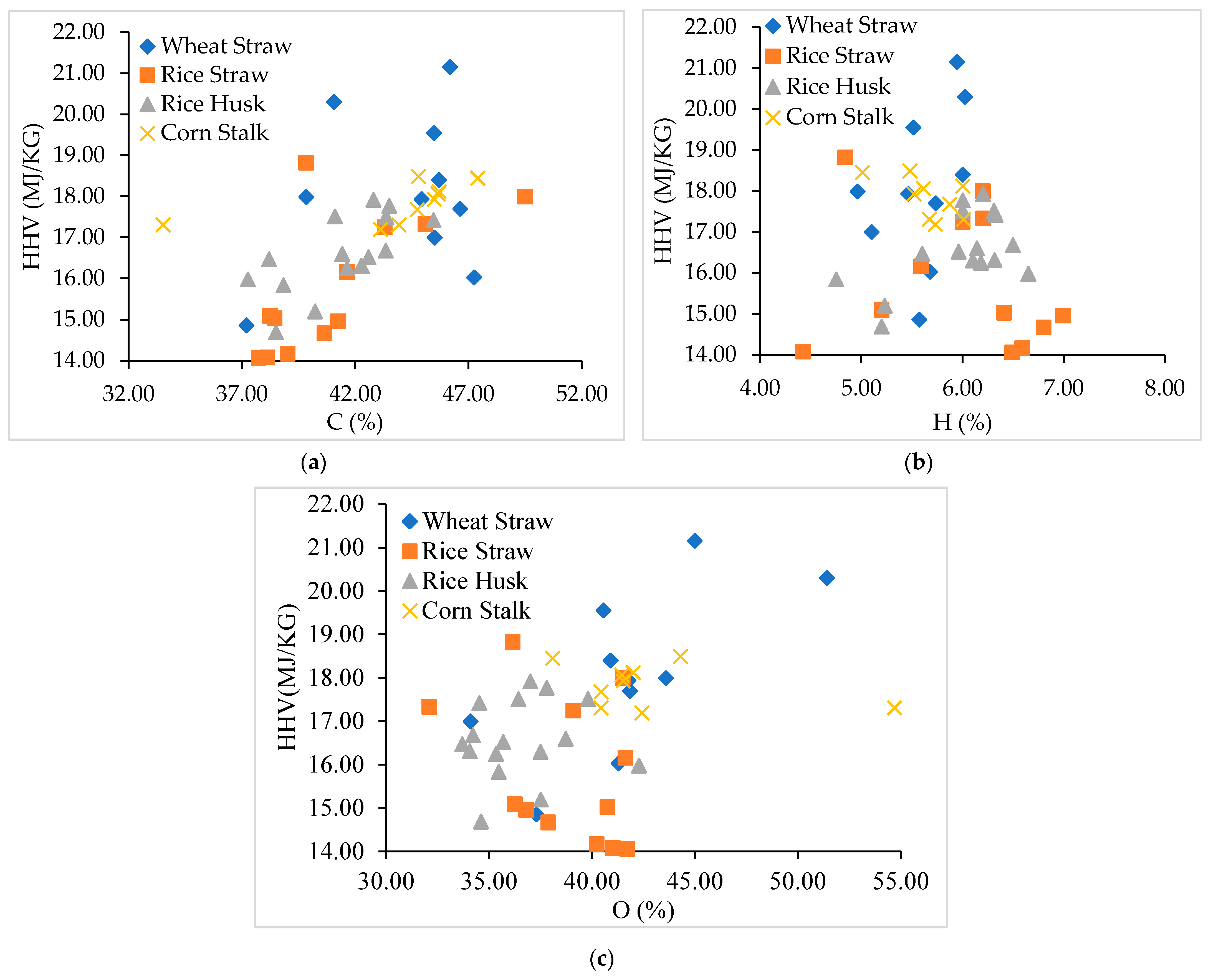
As shown in Figure 2, the HHV of the agricultural crop residue sample was firstly plotted as a function of the C, H, and O contents to identify the correlation between the HHV and the composition of the ultimate analysis. The C content of agricultural crop residues was in the range of 33.52–49.50%, the H content was in the range of 4.42–6.99%, and the O content was in the range of 32.10 to 54.69%. The HHV was between 14.06 MJ/kg and 21.16 MJ/kg. Agricultural crop residues have relatively lower C contents and higher H contents than fossil fuels (e.g., coal), which results in the higher content of O and a lower HHV [39,41]. The C content in agricultural crop residues was lower than the reported C content in biomass, which is in the range of 42–71% due to the higher ash content [16]. The average HHVs of WS, RS, RH, and CS were 18.09 MJ/kg, 15.62 MJ/kg, 16.56 MJ/kg, and 17.84 MJ/kg, respectively. It can be seen that WS and CS have relatively higher HHVs than the rice-crop-related residues, RS and RH. A possible reason for this may be that rice cultivation requires more water than the growing seasons of wheat and corn, which induced higher inherent moisture content and lower HHV in rice. The HHV results of the agricultural crop residues in this study are slightly higher than the reported HHV of the agricultural biomass, which ranged from 12.00 MJ/kg to 20.00 MJ/kg, probably because only the reported values from agricultural crops including southern pine, rice straw, cotton stalk, and corn stover were selected and WS, which has the potential to yield the highest HHV, was not included in previous studies [42].

A clear trend can be observed that the HHV of the selected agricultural crop residues were increased by the increasing percentages of C, which was also observed by Callejón-Ferre et al. [43] and Telmo et al. [44]. A similar trend can be seen in that the concentration of O was positively correlated to HHV. Compared with the C and O contents, the relationship between the HHV and the H content was not very clear. Hydrogen plays an important role in all fuel combustion system, and the greater the H + C/O ratio of a fuel, the greater the HHV was expected to be [45]. Nevertheless, it was found that the H + C/O ratio for WS, RS, RH, and CS was 1.20, 1.17, 1.30, and 1.17, respectively. Contrary to the work of Demirbas [45], RH, which has the highest H + C/O ratio, had a relatively lower HHV than other fuels. It is inferred that the relationship between H and HHV is more complicated, and linear regression models may not be suitable to precisely estimate the HHV of agricultural crop residues. Therefore, nonlinear models and combinations of linear and nonlinear regression models with interaction effects were also suggested to develop more accurate HHV models.

Table 6. Summary of developed linear and non-linear regression models for agricultural crop residues.

Fuel Type	No.	Developed New HHV Regression Models	R2
			%
All	N1	HHV = −1.41 + 0.3056 C − 0.145 H + 0.1557 O	62.26
All	N2	HHV = 47.7 + 0.2642 C − 31.5 H + 0.1410 O + 6.61 H2 − 0.446 H3	68.26
All	N3	HHV = −12.8 + 0.113 C − 4.8 H + 0.631 O + 2.48 H2 − 0.214 H3 + 0.024 CH − 0.083 HO	69.00
All	N4	HHV = −7 + 0.485 C + 6.7 H − 1.39 O + 0.98 H2 − 0.122 H3 − 0.038 CH − 0.1121 HO + 0.033 O2 − 0.00009 O3	77.67
WS	N5	HHV = −1.86 + 0.179 C − 0.22 H + 0.314 O	62.87
WS	N6	HHV = −2206 + 0.189 C + 1242 H + 0.237 O − 232 H2 + 14.4 H3	80.29
WS	N7	HHV = −9593 − 20.6 C + 5640 H − 7.88 O − 1055 H2 + 63.1 H3 + 3.71 CH + 1.460 HO	95.03
RS	N8	HHV = 6.29 + 0.2754 C − 0.576 H + 0.0377 O	73.96
RS	N9	HHV = 88.6 + 0.2937 C − 47.8 H − 0.0748 O + 9.12 H2 − 0.572 H3	93.61
RS	N10	HHV = −65.4 − 0.465 C + 26.5 H + 0.992 O − 2.98 H2 + 0.095 H3 + 0.119 CH − 0.170 HO	97.09
RH	N11	HHV = −0.76 + 0.2602 C + 0.518 H + 0.0932 O	56.76
RH	N12	HHV = −955 + 0.263 C + 477 H + 0.0805 O − 79.0 H2 + 4.34 H3	75.33
RH	N13	HHV = −1060 − 3.38 C + 583 H − 0.36 O − 101.3 H2 + 5.57 H3 + 0.603 CH + 0.097 HO	82.74
CS	N14	HHV = −4.69 + 0.3810 C − 0.238 H + 0.1636 O	93.31
CS	N15	HHV = −9 +0.3586 C + 7 H +0.1980 O − 2.1 H2 + 0.18 H3	94.93
CS	N16	HHV = −23 + 4.9 C − 77 H + 0.309 O + 21 H2 − 1.34 H3 − 0.78 CH	95.42

summarizes the developed sixteen HHV models along with the R² for all types of agricultural crop residues, and individual WS, RS, RH, and CS based on three major elemental composition from the ultimate analysis. The letter “N” presents the new models derived from this study and letter “E” represents the existing models from previous studies. Results indicated that R² ranged from 62.26% to 77.67%, 62.87% to 95.03%, 73.96% to 97.09%, 56.76% to 82.74%, and 93.31% to 95.42% for all types, WS, RS, RH, and CS, respectively. The R² of the HHV models developed from the sample dataset of individual agricultural crop residue types, such as WS, RS, RH, and CS, were larger than all types (i.e., mixture of selected four agriculture crop residues). This result showed that existing HHV models used a large range of data sets within all types of agricultural crop residues (the highest R² of 78%) were not accurate and are not applicable for the individual agricultural fuel types (the highest R² of 97%) [39]. Results showed that new regression models, N7, N10, N13, and N16, had the highest R² to predict the HHV of WS, RS, RH, and CS, respectively. In addition, the integration of quadratic and cubic effects of H, the interaction effect between H and O, H, and C, as well as the quadratic and cubic effects of O into the linear regression model increased R² and improved the accuracy of the HHV prediction models.

As shown in Figure 3, e and f shows that the predicted HHV results from the existing ultimate analysis-based models (E4 and E10) with three major components were deviated significantly from the line, where the predicted HHV and the measured HHV is equal (HHV_predicted = HHV_experimental (see red lines in Figure 3)). This observation confirmed that the existing models are not suitable in estimating the HHV of agricultural crop residues. On the contrary, the results from Figure 3a–d indicated that the estimated HHV results from new regression models (N1, N2, N3, and N4) were relatively close to the line of HHV_predicted = HHV_experimental, indicating high accuracy for HHV predictions of agricultural crop residues. These results further explained that the newly developed models (i.e., N1 to N4) had better accuracy than the existing HHV models (e.g., E3 and E10) in the HHV estimation of the agricultural crop residues. It is obvious that the predicated HHV results from the best-fit regression model (N4) and the measured HHV results from the adiabatic bomb calorimeter experiment are very close. Results showed that the best-fit regression model (N4) only slightly overestimated or underestimated the actual measured HHVs.

Validations were performed for the new regression models, N1 to N4 (for all types of agricultural crop residues), to ensure the compatibility with other agricultural crop residue samples with different characteristics and from different farming practices and geological locations. As shown in Figure 4, the estimation errors, AAE and ABE, of the ultimate-analysis-based new regression models (N1 to N4) and existing models (E1 to E11, from Table 1) were calculated by using the additional four agricultural crop residue samples (no. 11 WS, no. 6 RS, no. 1 RH and no. 14 CS). Results showed the new regression models posed an AAE of 4.50 to 6.28% and an ABE of −0.34 to 4.33% while existing models had an AAE of 6.87 to 18.87% and an ABE of −1.28 to 18.87%. Overall, the results showed that the new HHV models had higher accuracy and lower estimation errors than the existing HHV models. It was not surprising that the estimation errors from the existing models were relatively very high because the coefficients of the mathematical HHV models were different and concentrations of proximate analysis were also varied for each fuel [15]. AAE and ABE of the existing models, E3 (biomass), E4 (sewage sludge), E6 (MSW), E7 and E10 (biomass), and E11 (any fuel), were overestimated compared to the measured HHV (AAE > 10% and ABE > 5%) because they were developed for any fuels and developed using the wide ranges of biomass samples, which included woody biomass, MSW, sewage sludge, etc. It confirmed that the selected samples from a wide range of biomass types and species caused large variations on HHV prediction. Therefore, the newly developed regression models can be used to predict the HHV of agricultural crop residues with lower AAE and AEB.

3.2. Specific Heat Estimation

Table 7. Fuel properties of agricultural crop residues.

Fuel Type	C (wt%)	H (wt%)	O (wt%)	S (wt%)	N (wt%)	Ash (wt%)
Wheat Straw	43.97	5.60	41.78	0.18	0.79	7.16
Rice Straw	39.66	5.76	39.31	0.20	0.88	14.33
Rice Husk	41.42	5.97	36.54	0.08	0.48	15.62
Corn Stover	43.81	5.66	42.82	0.17	0.84	6.08

summarizes the average concentrations of the C, H, O, S, N, and ash content for the agricultural crop residue, including WS, RS, RH, and CS. Results indicated there was significant difference between fuel properties among the types of agricultural crop residues due to effect of species, farming practice, cultivation period, and geological location. It can be seen that WS and CS had almost twice the amount of ash than RS and RH that affected the amounts and compositions of the flue gas during combustion process.

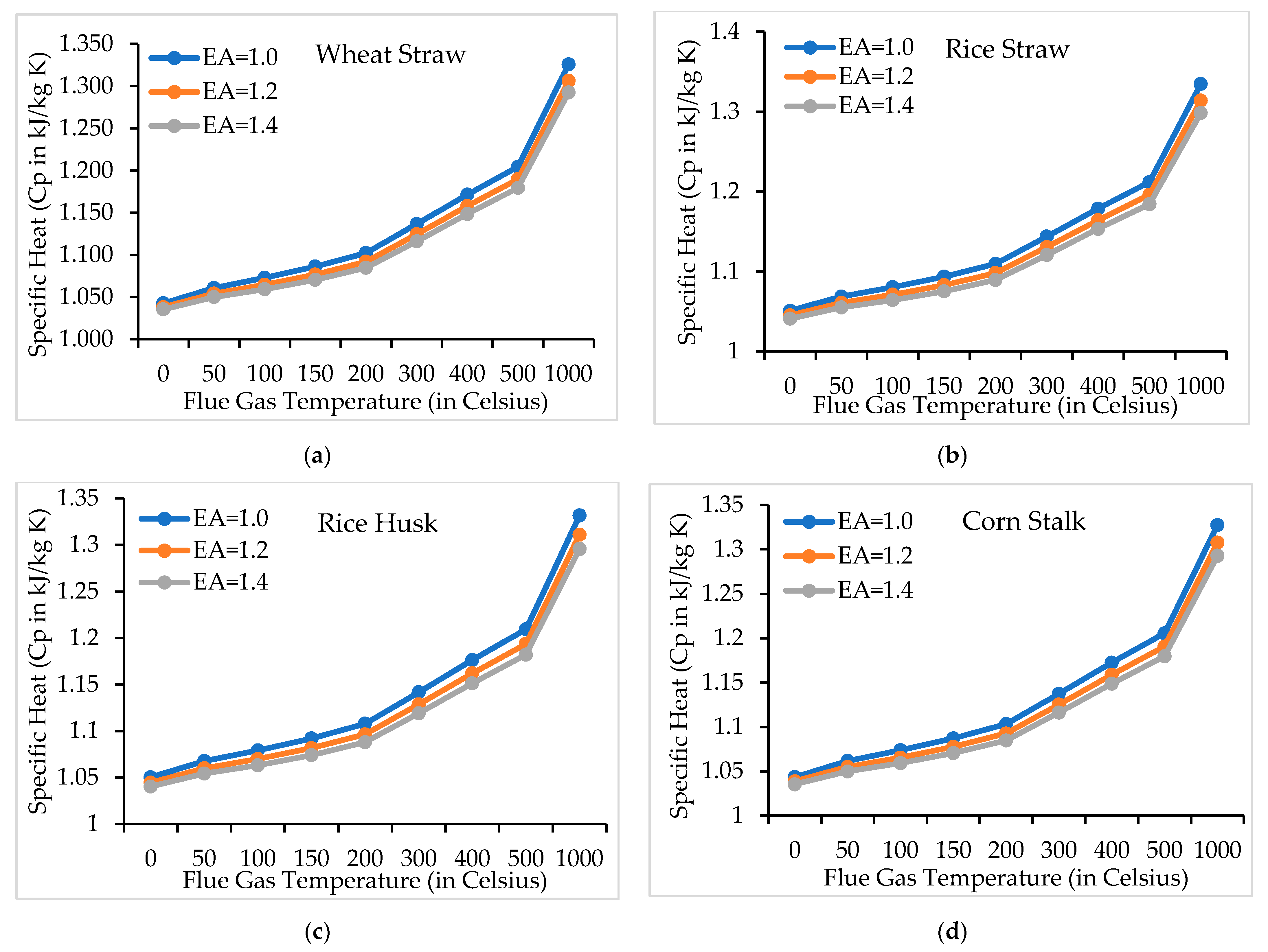
As shown in Figure 5, the specific heat of flue gas during the agricultural crop residue combustion was then predicted based on the calculated fuel properties under the various EA ratios and flue gas temperatures. The ranges of specific heat were 1.033 kJ/kg·K–1.326 kJ/kg·K, 1.039 kJ/kg·K–1.335 kJ/kg·K, 1.038 kJ/kg·K−1.332 kJ/kg·K, 1.034 kJ/kg·K–1.327 kJ/kg·K for WS, RS, RH, and CS, respectively. There were slight differences within the same EA and combustion temperature range because the fuel properties of the selected fuels (e.g., C, H, O, S, and ash) were different and caused variation in the mass fraction of the major combustion products. The specific heat of agricultural crop residue combustion was found to have a range of 1.033 kJ/kg·K to 1.327 kJ/kg·K, which was slightly smaller than the specific heat of natural gas combustion (1.11 kJ/kg·K to 1.43 kJ/kg·K) due to the lower C and H contents in agricultural crop residues. Moreover, the specific heat of agricultural crop residue combustion had smaller values than the specific heat of flue gas during poultry litter and natural gas co-combustion ranging between 1.044 kJ/kg·K and 1.338 kJ/kg·K [20]. Increment of EA ratios from 1.0 to 1.4 was found to decrease specific heat of flue gas. Coskun et al. [17] and Qian et al. [20] also investigated the influence of EA ratios on the specific heat of flue gas during the combustion process of fossil fuels, including natural gas, fuel oil, flame coal as well as biomass, such as poultry litter. These studies made similar conclusions that the specific heat of flue gas was decreased by increasing EA for both biomass and fossil fuels. A possible explanation can be that the increasing EA decreased the composition of H₂O and CO₂ while increased the percentage of O₂ among the flue gas. It is well known that both H₂O and CO₂ had a higher specific heat than the O₂. On the other hand, the specific heat of flue gas during the combustion process was raised by elevating the flue gas temperature from 0 °C to 1000 °C (equivalent to 273.15 to 1273.15 K). As the flue gas heated up at higher temperatures, vibrational and kinetic energy increased and required more thermal energy and ultimately raised specific heat values [20]. It was not surprising that the effect of EA and flue gas temperature on specific heat were opposite, because EA normally lowers flame temperature and combustion efficiency. Many previous research studies concluded that flue gas temperature and EA had an opposite relationship during the biomass and fossil fuel combustion process [46,47]. Our results confirm that flue gas from biomass combustion had higher specific heat than the air because the biomass combustion had a higher portion of H₂O and CO₂ [20].

3.3. Combustion Related Problems Prediction

As shown in

Table 8. Summary of fuel indices results and associated combustion problems.

No.	Fuel Type	2S/Cl	Corrosion Level	Sum of K+Na (mg/kg)	PM1.0 Level	K + Na/3(2S + Cl)	HCl & SOx Level	Si + P + K/Ca + Mg	Ash Melting Temp.
1	WS	0.79	S	7171	M	0.58	Elevated	5.0	Reduced
2		0.98	S	6912	M	0.38	Elevated	5.2	Reduced
3		1.57	S	2323	M	0.56	Elevated	12.5	Reduced
5		0.38	S	31,021	H	0.62	Elevated	6.9	Reduced
7		1.39	S	19,172	H	1.16	Reduced	11.4	Reduced
12		0.43	S	15,800	H	0.50	Elevated	10.1	Reduced
3	RS	0.62	S	24,756	H	0.88	Elevated	18.6	Reduced
4		1.00	S	19,455	H	1.62	Reduced	22.9	Reduced
5		0.30	S	23,550	H	0.99	Elevated	17.0	Reduced
14		0.31	S	38,665	H	0.96	Elevated	16.4	Reduced
1	RH	0.83	S	7942	M	1.20	Reduced	29.7	Reduced
5		1.67	S	3664	M	0.76	Elevated	122.6	Reduced
18		0.40	S	7168	M	0.85	Elevated	46.1	Reduced
8	CS	0.22	S	12,424	H	0.53	Elevated	3.3	Reduced
11		0.81	S	14,597	H	2.73	Reduced	7.8	Reduced
12		0.50	S	8220	M	0.51	Elevated	2.4	Reduced

Note: S = Severe; M = Medium; H = High.

, the fuel indices of individual samples were calculated and associated combustion problems, including the corrosion level, PM_1.0 level, HCl and SO_x level, and ash melting temperature, were predicted based on the evaluation standards. These results showed that the range of fuel indices were widely dispersed within the different fuel types of agricultural crop residues as well as within the same fuel type due to various fuel properties, farming practices (e.g., storage, harvest, and cultivation), and regional differences. It can be concluded that agriculture crop residues have a severe risk of corrosion because they have a relatively high amount of ash (about 6–15%) and chlorine (up to around 1%) [5]. High amounts of Cl reacted with evaporated alkali metals (e.g., K, Na) from ash to form alkali chlorides (e.g., KCl and NaCl), which reacted with SO₂ and O₂ to form sulphates (e.g., Na₂SO₄ and K₂SO₄) as deposits and released gaseous Cl₂ during the combustion process. Generated Cl₂ gas reacted with the low alloy steel (e.g., Cu and Fe) to form FeCl₂, which diffused through the deposit layer via a significant vapor pressure and reacted with excess oxygen to produce metal oxides (i.e., Fe₂O₃ or Fe₃O₄) and regenerated Cl₂ again, resulting in severe corrosion and active oxidation [5]. The reduced ash melting temperature on all types of agriculture crop residues can be explained by the presence of several key binary salt mixtures, particularly KCl-FeCl₂ and NaCl-FeCl₂, which have low temperature eutectics in the range of 340–390 °C compared to the pure compounds (e.g, NaCl with 800 °C, and FeCl₂ with 677 °C) within the chloride-rich biomass ash [5,48]. Results also showed that the change of gaseous emissions, PM_1.0 emissions, and HCl and SO_x emissions were slightly different and not obvious.

As shown in Figure 6, the average 2S/Cl index was 0.87, 0.85, 0.34, and 0.81 for WS, RS, RH and CS, respectively. This confirmed that 2S/Cl values for all types of agricultural crop residues were lower than two, which would cause a Cl surplus in aerosols prevailing and severe corrosion on the surface of combustion units and heat exchangers during the combustion process. Comparison among the four different agricultural biomasses showed that RS had the highest sum of K + Na, indicating the highest PM_1.0 emissions because RS had an approximately three to six times higher amount of K and a four to nine times higher amount of Na than the three other agricultural biomass fuels. Therefore, higher K and Na generated more alkali metal chlorides (e.g., KCl and NaCl) and sulphates (e.g., Na₂SO₄ and K₂SO₄) to form PM_1.0 emissions [32]. In addition, the fuel indices of PM_1.0 for WS, RH, and CS were also higher than 10,000 mg/kg, suggesting that all agricultural crop residues were expected to have a high PM_1.0 emission range (>100 mg/MJ) [35]. This finding was consistent with previous results that PM_1.0 is one of the major gases emissions and that there is a critical need of both primary and secondary measures to capture PM_1.0 emissions during the agricultural biomass combustion process [4,12]. In addition, RS had the highest (K + Na)/3(2S + Cl) and produced the lowest SO₂ and HCl emissions because the SO₂ emission reacts with alkali metals, and the regeneration of Cl₂ occurs via the active oxidation instead of HCl emission [5]. Compared with WS and CS, rice-related residues showed higher ash indices and lower ash sintering temperatures because RS and RH had higher Si that may have formed excess SiO₂ and resulted in a porous structure that ultimately decreased the sintering temperature [49]. In most studies, the ultimate analysis of major elements (e.g., C, H, O, N, and S) were identified using the elemental analyzer based standard methods (e.g., ASTEM, EN-ISO) in the combustion studies to investigate the combustion performance and emissions (e.g., CO, SO₂, and NO_x) [14]. However, the composition analysis of Cl was neglected in the majority studies in spite of the fact that the Cl concentration was critical in predicting the HCl emissions and corrosion problems. According to some authors, Cl was involved in the elemental analysis and determined using standard ASTM E776-87 [16]. It is recommended that the concentration of inorganic components (e.g., Cl, K, Na, Si, Ca, Mg, and P) should be measured to predict combustion-related problems before the actual combustion test.

4. Conclusions

Increasing energy demand, availability of a number of varieties of biomass, and the low cost of the agricultural crop residues has stimulated the replacement of fossil fuels with the alternative energy resources that produce energy in an environment-friendly, sustainable, and cost-effective means. Thermal properties, including higher heating value (HHV), specific heat, and combustion-related problems (e.g., gaseous emissions and ash related problems) were characterized and predicted using the integration of the HHV model, specific heat model, and fuel indices as a new systematic approach. Four representative agricultural crop residues, namely wheat straw (WS), rice straw (RS), rice husk (RH), and corn stalk (CS) were selected. Sixteen HHV models based on the ultimate analysis results were developed and validated to have a lower estimation error and higher R² values than the existing models to predict the HHV of agricultural crop residues. This study also predicted the specific heat of flue gas during the agricultural crop residue combustion process based on the fuel properties, EA, and flue gas temperature. It was found that specific heat was affected by fuel properties and decreased with increasing EA and decreasing flue gas temperature, while the specific heat of flue gas during the agricultural crop residue combustion process was lower than that of fossil fuels and higher than air. Four fuel indices were calculated and used to study the corrosion, PM_1.0 emissions, HCl and SO_x emissions, and ash sintering temperature. Agricultural crop residues were found to have severe corrosion risk and lower ash sintering temperatures. This study showed the possibility to characterize and pre-evaluate the combustion-related properties and associated problems by integrating of the HHV models, specific heat models, and fuel indices. For practical significance and usefulness, this study developed HHV models that can be used to estimate the HHV values of agricultural crop residues, including the barely, sorghum, oil crops, and sugar crop from the ultimate analysis. In addition, this integration evaluation approach, including the HHV model, specific heat model, and fuel indices can be used to determine thermal properties (e.g., HHV, specific heat) and combustion problems (e.g., PM_1.0, corrosion, HCl and SO₂ emissions) for biomass fuels (e.g., municipal solid waste, industrial residues, and animal residues). The HHV and specific heat value are also very important to model biomass combustion process. In future studies, additional biomass samples, such as short rotation energy crops, industrial wastes, and municipal solid wastes, can be collected and pre-evaluated to predict the thermal properties and combustion problems of various biomass fuels, improve energy production, reduce emissions during the combustion process, and increase utilization of biomass fuels.

References

- Conti, J.; Holtberg, P.; Diefenderfer, J.; LaRose, A.; Turnure, J.T.; Westfall, L. International Energy Outlook 2016 With Projections to 2040; Government Printing Office: Washington, DC, USA, 2016. [CrossRef] [Green Version]
- Saidur, R.; Abdelaziz, E.A.; Demirbas, A.; Hossain, M.S.; Mekhilef, S. A review on biomass as a fuel for boilers. Renew. Sustain. Energy Rev. 2011, 15, 2262–2289. [Google Scholar] [CrossRef]
- Demirbas, A. Prediction of higher heating values for vegetable oils and animal fats from proximate analysis data. Energy Source Part A 2009, 31, 1264–1270. [Google Scholar] [CrossRef]
- Brassard, P.; Palacios, J.H.; Godbout, S.; Bussières, D.; Lagacé, R.; Larouche, J.P.; Pelletier, F. Comparison of the gaseous and particulate matter emissions from the combustion of agricultural and forest biomasses. Bioresour. Technol. 2014, 115, 300–306. [Google Scholar] [CrossRef] [PubMed]
- Koppejan, J.; Van Loo, S. The Handbook of Biomass Combustion and Co-Firing, Reprint; Earthscan: London, UK, 2010. [Google Scholar]
- Lal, R. World crop residues production and implications of its use as a biofuel. Environ. Int. 2005, 31, 575–584. [Google Scholar] [CrossRef] [PubMed]
- Cherubin, M.R.; Oliveira, D.M.D.S.; Feigl, B.J.; Pimentel, L.G.; Lisboa, I.P.; Gmach, M.R.; Cerri, C.C. Crop residue harvest for bioenergy production and its implications on soil functioning and plant growth: A review. Sci. Agric. 2018, 75, 255–272. [Google Scholar] [CrossRef] [Green Version]
- Ni, H.; Han, Y.; Cao, J.; Chen, L.W.A.; Tian, J.; Wang, X.; Li, H. Emission characteristics of carbonaceous particles and trace gases from open burning of crop residues in China. Atmos. Environ. 2015, 123, 399–406. [Google Scholar] [CrossRef]
- Sun, J.; Shen, Z.; Cao, J.; Zhang, L.; Wu, T.; Zhang, Q.; Liu, S. Particulate matters emitted from maize straw burning for winter heating in rural areas in Guanzhong Plain, China: Current emission and future reduction. Atmos. Res. 2017, 184, 66–76. [Google Scholar] [CrossRef]
- Demirbas, M.F.; Balat, M.; Balat, H. Potential contribution of biomass to the sustainable energy development. Energy Convers. Manag. 2009, 50, 1746–1760. [Google Scholar] [CrossRef]
- Yin, C.Y. Prediction of higher heating values of biomass from proximate and ultimate analyses. Fuel 2011, 90, 1128–1132. [Google Scholar] [CrossRef] [Green Version]
- Yang, W.; Zhu, Y.; Cheng, W.; Sang, H.; Yang, H.; Chen, H. Characteristics of particulate matter emitted from agricultural biomass combustion. Energy Fuel 2017, 31, 7493–7501. [Google Scholar] [CrossRef]
- Katsaros, G.; Sommersacher, P.; Retschitzegger, S.; Kienzl, N.; Tassou, S.A.; Pandey, D.S. Combustion of poultry litter and mixture of poultry litter with woodchips in a fixed bed lab-scale batch reactor. Fuel 2021, 286, 119310. [Google Scholar] [CrossRef]
- Cai, J.; He, Y.; Yu, X.; Banks, S.W.; Yang, Y.; Zhang, X.; Bridgwater, A.V. Review of physicochemical properties and analytical characterization of lignocellulosic biomass. Renew. Sustain. Energy Rev. 2017, 76, 309–322. [Google Scholar] [CrossRef] [Green Version]
- Qian, X.; Lee, S.; Soto, A.-M.; Chen, G. Regression model to predict the higher heating value of poultry waste from proximate analysis. Resources 2018, 7, 39. [Google Scholar] [CrossRef] [Green Version]
- Vargas-Moreno, J.M.; Callejón-Ferre, A.J.; Pérez-Alonso, J.; Velázquez-Martí, B. A review of the mathematical models for predicting the heating value of biomass materials. Renew. Sustain. Energy Rev. 2012, 16, 3065–3083. [Google Scholar] [CrossRef]
- Coskun, C.; Oktay, Z.U.H.A.L.; Ilten, N. A new approach for simplifying the calculation of flue gas specific heat and specific exergy value depending on fuel composition. Energy 2009, 34, 1898–1902. [Google Scholar] [CrossRef]
- Menghini, D.; Marra, F.S.; Allouis, C.; Beretta, F. Effect of excess air on the optimization of heating appliances for biomass combustion. Exp. Therm. Fluid Sci. 2008, 32, 1371–1380. [Google Scholar] [CrossRef]
- Chandok, J.S.; Kar, I.N.; Tuli, S. Estimation of furnace exit gas temperature (FEGT) using optimized radial basis and back-propagation neural networks. Energy Convers. Manag. 2008, 49, 1989–1998. [Google Scholar] [CrossRef]
- Qian, X.; Lee, S.W.; Yang, Y. Heat Transfer Coefficient Estimation and Performance Evaluation of Shell and Tube Heat Exchanger Using Flue Gas. Processes 2021, 9, 939. [Google Scholar] [CrossRef]
- Sheng, C.; Azevedo, J.L.T. Estimating the higher heating value of biomass fuels from basic analysis data. Biomass Bioenergy 2005, 28, 499–507. [Google Scholar] [CrossRef]
- Ghugare, S.B.; Tiwary, S.; Elangovan, V.; Tambe, S.S. Prediction of higher heating value of solid biomass fuels using artificial intelligence formalisms. Bioenergy Res. 2014, 7, 681–692. [Google Scholar] [CrossRef]
- Jenkins, B.M.; Ebeling, J.M. Correlations of physical and chemical properties of terrestrial biomass with conversion. In Proceedings of the 1985 Symposium Energy from Biomass and Waste IX Institute of Gas Technology, Chicago, IL, USA, 13–17 February 1985; pp. 371–400. [Google Scholar]
- Abe, F. The thermochemical study of forest biomass. Bull. For. For. Prod. Res. Inst. 1988, 352, 1–95. [Google Scholar]
- Elneel, R.; Anwar, S.; Ariwahjoed, B. Prediction of heating values of oil palm fronds from ultimate analysis. J. Appl. Sci. 2013, 13, 491–496. [Google Scholar] [CrossRef] [Green Version]
- Han, J.; Yao, X.; Zhan, Y.; Oh, S.Y.; Kim, L.H.; Kim, H.J. A method for estimating higher heating value of biomass-plastic fuel. J. Energy Inst. 2017, 90, 331–335. [Google Scholar] [CrossRef]
- Thipkhunthod, P.; Meeyoo, V.; Rangsunvigit, P.; Kitiyanan, B.; Siemanond, K.; Rirksomboon, T. Predicting the heating value of sewage sludges in Thailand from proximate and ultimate analyses. Fuel 2005, 84, 849–857. [Google Scholar] [CrossRef]
- Komilis, D.; Evangelou, A.; Giannakis, G.; Lymperis, C. Revisiting the elemental composition and the calorific value of the organic fraction of municipal solid wastes. Waste Manag. 2012, 32, 372–381. [Google Scholar] [CrossRef]
- Shi, H.; Mahinpey, N.; Aqsha, A.; Silbermann, R. Characterization, thermochemical conversion studies, and heating value modeling of Municipal Solid Waste. Waste Manag. 2016, 48, 34–47. [Google Scholar] [CrossRef] [PubMed]
- Schmidt-Rohr, K. Why combustions are always exothermic, yielding about 418 kJ per Mole of O2. J. Chem. Educ. 2015, 92, 2094–2099. [Google Scholar] [CrossRef] [Green Version]
- Merckel, R.D.; Labuschagne, F.J.W.J.; Heydenrych, M.D. Oxygen consumption as the definitive factor in predicting heat of combustion. Appl. Energy 2019, 235, 1041–1047. [Google Scholar] [CrossRef] [Green Version]
- Brunner, T.; Sommersacher, P.; Obernberger, I. Fuel indexes—A novel method for the evaluation of relevant combustion properties of new biomass fuels. In Proceedings of the 19th European Biomass Conference & Exhibition, Berlin, Germany, 6–10 June 2011; pp. 1351–1357. [Google Scholar]
- Sommersacher, P.; Brunner, T.; Obernberger, I. Fuel indexes: A novel method for the evaluation of relevant combustion properties of new biomass fuels. Energy Fuel 2012, 26, 380–390. [Google Scholar] [CrossRef]
- Sommersacher, P.; Brunner, T.; Obernberger, I.; Kienzl, N.; Kanzian, W. Application of novel and advanced fuel characterization tools for the combustion related characterization of different wood/kaolin and straw/kaolin mixtures. Energy Fuel 2013, 27, 5192–5206. [Google Scholar] [CrossRef]
- Obernberger, I.; Brunner, T. Advanced characterisation methods for solid biomass fuels. International Energy Agency Bioenergy Task 32 Report: 13-14. 2015. Available online: https://nachhaltigwirtschaften.at/resources/iea_pdf/reports/iea_bioenergy_task32_advanced_characterisation_methods_for_solid_biomass_fuels.pdf (accessed on 24 July 2021).
- Fournel, S.; Palacios, J.H.; Morissette, R.; Villeneuve, J.; Godbout, S.; Heitz, M.; Savoie, P. Influence of biomass properties on technical and environmental performance of a multi-fuel boiler during on-farm combustion of energy crops. Appl. Energy 2015, 141, 247–259. [Google Scholar] [CrossRef]
- Marangwanda, G.T.; Madyira, D.M.; Babarinde, T.O. Combustion models for biomass: A review. Energy Rep. 2020, 6, 664–672. [Google Scholar] [CrossRef]
- Albrecht, B.A.; Bastiaans, R.J.M.; Van Oijen, J.A.; De Goey, L.P.H. NOx emissions modelling in biomass combustion grate furnaces. In Proceedings of the 7th European Conference on Industrial Furnaces and Boilers, Porto, Portugal, 18–21 April 2006. [Google Scholar]
- Nhuchhen, D.R.; Afzal, M.T. HHV Predicting Correlations for Torrefied Biomass Using Proximate and Ultimate Analyses. Bioengineering 2017, 4, 7. [Google Scholar] [CrossRef] [Green Version]
- Cengel, Y. Heat and Mass Transfer: Fundamentals and Applications; McGraw-Hill Higher Education: New York, NY, USA, 2014. [Google Scholar]
- Vassilev, S.V.; Vassileva, C.G.; Vassilev, V.S. Advantages and disadvantages of composition and properties of biomass in comparison with coal: An overview. Fuel 2015, 158, 330–350. [Google Scholar] [CrossRef]
- Adhikari, S.; Nam, H.; Chakraborty, J.P. Conversion of solid wastes to fuels and chemicals through pyrolysis. Waste Biorefinery 2018, 239–263. [Google Scholar] [CrossRef]
- Callejón-Ferre, A.J.; Velázquez-Martí, B.; López-Martínez, J.A.; Manzano-Agugliaro, F. Greenhouse crop residues: Energy potential and models for the prediction of their higher heating value. Renew. Sustain. Energy Rev. 2011, 15, 948–955. [Google Scholar] [CrossRef]
- Telmo, C.; Lousada, J.; Moreira, N. Proximate analysis, backwards stepwise regression between gross calorific value, ultimate and chemical analysis of wood. Bioresour. Technol. 2010, 101, 3808–3815. [Google Scholar] [CrossRef] [PubMed]
- Demirbas, A. Relationships between heating value and lignin, moisture, ash and extractive contents of biomass fuels. Energy Explor. Exploit. 2002, 20, 105–111. [Google Scholar] [CrossRef]
- Houshfar, E.; Skreiberg, Ø.; Løvås, T.; Todorović, D.; Sørum, L. Effect of excess air ratio and temperature on NOx emission from grate combustion of biomass in the staged air combustion scenario. Energy Fuel 2011, 25, 4643–4654. [Google Scholar] [CrossRef]
- Qian, X. Statistical Analysis and Evaluation of the Advanced Biomass and Natural Gas Co-Combustion Performance. Ph.D. Thesis, Morgan State University, Baltimore, MD, USA, 2019. [Google Scholar]
- Nielsen, H.P.; Frandsen, F.J.; Dam-Johansen, K.; Baxter, L.L. The implications of chlorine-associated corrosion on the operation of biomass-fired boilers. Prog. Energy Combust. Sci. 2000, 26, 283–298. [Google Scholar] [CrossRef]
- Hu, H.; Zhou, K.; Meng, K.; Song, L.; Lin, Q. Effects of SiO2/Al2O3 ratios on sintering characteristics of synthetic coal ash. Energies 2017, 10, 242. [Google Scholar] [CrossRef] [Green Version]