
The IRC-PD Tool: A Code to Design Steam and Organic Waste Heat Recovery Units


1
LGPDDPS Laboratory, Department of Process Engineering, National Polytechnic School of Constantine (ENPC), BP 75, Ali Mendjeli, Constantine 25000, Algeria
2
Department of Industrial Engineering, University of Padova, Via Venezia 1, 35131 Padova, Italy
*
Author to whom correspondence should be addressed.
Energies 2021, 14(18), 5611; https://0-doi-org.brum.beds.ac.uk/10.3390/en14185611
Submission received: 11 July 2021
/
Revised: 17 August 2021
/
Accepted: 1 September 2021
/
Published: 7 September 2021
(This article belongs to the Special Issue Industry and Tertiary Sectors towards Clean Energy Transition)
Abstract
:The Algerian economy and electricity generation sector are strongly dependent on fossil fuels. Over 93% of Algerian exports are hydrocarbons, and approximately 90% of the generated electricity comes from natural gas power plants. However, Algeria is also a country with huge potential in terms of both renewable energy sources and industrial processes waste heat recovery. For these reasons, the government launched an ambitious program to foster renewable energy sources and industrial energy efficiency. In this context, steam and organic Rankine cycles could play a crucial role; however, there is a need for reliable and time-efficient optimization tools that take into account technical, economic, environmental, and safety aspects. For this purpose, the authors built a mathematical tool able to optimize both steam and organic Rankine units. The tool, called Improved Rankine Cycle Plant Designer, was developed in MATLAB environment, uses the Genetic Algorithm toolbox, acquires the fluids thermophysical properties from CoolProp and REFPROP databases, while the safety information is derived from the ASHRAE database. The tool, designed to support the development of both RES and industrial processes waste heat recovery, could perform single or multi-objective optimizations of the steam Rankine cycle layout and of a multiple set of organic Rankine cycle configurations, including the ones which adopt a water or an oil thermal loop. In the case of the ORC unit, the working fluid is selected among more than 120 pure fluids and their mixtures. The turbines’ design parameters and the adoption of a water- or an air-cooled condenser are also optimization results. To facilitate the plant layout and working fluid selection, the economic analysis is performed to better evaluate the plant economic feasibility after the thermodynamic optimization of the cycle. Considering the willingness of moving from a fossil to a RES-based economy, there is a need for adopting plants using low environmental impact working fluids. However, because ORC fluids are subjected to environmental and safety issues, as well as phase out, the code also computes the Total Equivalent Warming Impact, provides safety information using the ASHRAE database, and displays an alert if the organic substance is phased out or is going to be banned. To show the tool’s potentialities and improve the knowledge on waste heat recovery in bio-gas plants, the authors selected an in-operation facility in which the waste heat is released by a 1 MWel internal combustion engine as the test case. The optimization outcomes reveal that the technical, economic, environmental, and safety performance can be achieved adopting the organic Rankine cycle recuperative configuration. The unit, which adopts Benzene as working fluid, needs to be decoupled from the heat source by means of an oil thermal loop. This optimized solution guarantees to boost the electricity production of the bio-gas facility up to 15%.
1. Introduction
The availability of cheap energy is a key factor in the socio-economic development of the humankind. However, the ever-growing population and the subsequent continuous rise of the energy demand is boosting the human-caused carbon dioxide (CO2) emissions at an yearly rate ranging from 0.5% to 2%, an unsustainable trend of growth considering that it is well-known that CO2 and other greenhouse gases (GHGs) emissions are one of the driver of the global climate change [1]. Thus, to fight GHGs effects and meet the ambitious target of limiting global warming to “well below” 2 °C above pre-industrial levels [1], there is an urgent need to shift from a fossil- to a renewable-based energy generation system, as well as supporting the energy efficiency implementation, at least at the industrial level. In fact, the efficient use of energy in the industrial sector is a cornerstone because, based on the International Energy Agency (IEA) estimations, it is the largest producer of CO2, with over 21.4 Gton [2]. This quantity is not equally shared by neither the industries nor the countries. The power industry (25%), the iron and steel production (7.2%), the cement manufacturing (5%), and the chemicals and petrochemicals (3.6%) are responsible for approximately 40% of the global CO2 emissions, while Japan (32%), China (28%), US (15%), and India (7%) contribute to over 80% of the total [2]. As known, the CO2 emissions are the result of the heavy usage of combustion processes adopting oil, natural gas and coal as fuel [3], a fact that highlights the still poor penetration in the industrial sector of low-carbon and renewable-based generation options. However, CO2 and GHGs are not the unique emissions of the industrial sector because, due to the lack of waste heat recovery units (WHRUs), the sector largely also contributes to thermal pollution. Therefore, to substitute conventional fuels, secure the production, and abate the pollutants, there is a need to simultaneously support the spread of renewable energy source (RES) plants and waste heat recovery units.
In this context, the European Union (EU) is the leading region because (i) it is reaching its GHG emissions reduction targets set for 2020, (ii) it has planned to further cut emissions by at least 55% by 2030, and (iii) it aims to become the world’s first climate-neutral continent by 2050 [4,5]. However, despite the EU ambitious goals, global warming and environmental pollution need to be counteracted at a worldwide level, particularly in countries extremely dependent on fossil resources, as well as rich of RES and processes with high energy recovery potential.
This is the case of Algeria, the largest African country in surface area, the gate of the African continent, and a strategic hub for shipping raw materials to EU. Currently, the country’s economy is extremely dependent on fossil fuels because oil and natural gas constitute the 93.6% of its export. In addition, the electricity generation sector is strictly bounded to fossil resources; 90% of the electricity is generated in thermal power plants fed by natural gas. In addition, the Algerian soil hosts several energy intensive and large pollutants emitter industries, such as the cement manufacturing.
However, regardless the current structure of the power industries, the country can easily meet its national energy demand by exploiting the considerable RES and waste heat recovery potential [6]. In fact, looking the country’s map, it is clear that the major contribution to electricity production can be supplied by solar photovoltaic (PV) installations because the Saharan region, which covers approximately the 86% of the Algerian soil, can meet the national demand, as well as part of the EU one, thanks to an average energy and sunshine duration of 2650 kWh m−2 per year and 3500 h per year, respectively [7]. However, to move toward a renewable and sustainable energy generation mix able to (i) cut 193 million tons of CO2 by 2030 [6], (ii) shift Algeria from the third most significant emitters of CO2 among the African countries to the forefront of the climate-neutral ones [8], and (iii) free up energy resources for export [8], it is also mandatory to exploit wastes, such as biomass fermentable substances and the waste heat released by industrial processes, RES plants, etc.
To this end, it is important to highlight that biomass fermentable resources can play a crucial role not only in the Algerian energy mix but also in the country’s waste management. In 2014, the household and similar wastes sent to landfill reached 14 million tons, and, among them, 8.7 million tons could be used for energy purposes [9]. Therefore, thanks to the anaerobic digestion process, the 8.7 million tons of fermentable biomass can produce 974 million cubic meter of bio-gas, a volume that could generate at least 1685 GWh of electricity, which, in turn, could cover the annual demand of approximately one million of Algerian inhabitants [9]. In this context, it is clear that, for recovering energy from both industrial processes (see, e.g., References [10,11,12,13,14]) and RES (see, e.g., References [15,16,17,18,19]), the major obstacle is the availability of flexible and time-efficient tools able to properly select the waste heat recovery unit type and design it (plant scheme, as well as devices characteristics, such as turbine type (axial or radial), heat exchanger dimensions, etc.) without requiring modifications, regardless of the heat source, in terms of type, mass flow, and temperature.
To this end, the authors developed the “Improved Rankine Cycle Plant Designer” (IRC-PD), an optimization tool able to design and select the most suitable WHRU between the steam and the organic Rankine cycles (SRC and ORC). In this manner, the tool can provide the WHRU design for each heat source type (liquid or gas) and temperature range (from high to low temperature). The SRC layout implemented in the code is a base one, given the WHRU aim of simplicity the cost-effectiveness, while the ORC configuration is selected among a multiple set of layouts, including the ones which adopt a water or an oil thermal loop, and the working fluid is selected among more than 120 pure fluids and their mixtures. For both SRC and ORC, the optimizer selects the most suitable turbine configuration (single or multi-stage and axial or radial) and condenser type (water- or air-cooled), as well as provides a preliminary design of the entire set of devices that make up the WHRU. Then, according to the optimization goal, which can be single or multiple (e.g., maximum design power), the IRC-PD tool ranks the solutions, and, for each of them, it performs an economic and a safety analysis. Finally, the tool provides a series of maps in which the most promising WHRU design characteristics are classified based on plant safety. To the authors’ knowledge, the aforementioned features are points of novelty because in literature no one has integrated into an unique optimization tool (i) the selection and design of both SRC and ORC units considering different plant layouts (including thermal loop) and pure working fluids and their mixtures, (ii) the preliminary design of the expander in both axial and radial configurations, (iii) the condenser type selection, and (iv) the economic and safety analyses.
To test the code ability of selecting the most performing WHRU, the authors choose an internal combustion engine (ICE) fed by bio-gas as a test case. This choice is driven by (i) the Algerian’s researchers need to evaluate the waste heat recovery potential in the bio-gas sector and (ii) the Italian’s researchers need to improve the knowledge in the ICE’s waste heat recovery potential, considering SRC and different ORC configurations. As said, the bio-gas production can be a way for Algeria to both produce electricity near the users and properly manage the fermentable wastes, while, for the Italian bio-gas market, this analysis can help in the further development of a strategic renewable resource, especially after the cessation of feed-in tariffs. In this regard, it is important to highlight that WHRUs in Italian bio-gas plants are rare; therefore, for Algerian and Italian bio-gas ICEs, this study can (i) point out the energetic and environmental benefits, (ii) push the legislator to promote the use of such technologies, (iii) help in the development of new production changes, and (iv) exchange knowledge between two countries with a strategic role in the Mediterranean Sea.
The rest of the work is organized as follows. In Section 2, the IRC-PD tool is presented in detail, while its validation is summarized in Section 3. Section 4 describes the selected case study and the tool settings, while the outcomes of the optimization process are presented and discussed in Section 5. Finally, the concluding remarks are given in Section 6.
2. The Improved Rankine Cycle Plant Designer—IRC-PD
The Improved Rankine Cycle Plant Designer is the result of a joint research between the University of Padova (Italy) and the National Polytechnic School of Constantine (Algeria). The IRC-PD tool, which was developed in MATLAB environment [20], is an “in-house” optimization code able to design two kinds of waste heat recovery unit: the one adopting the steam Rankine cycle and the WHRU operating with the organic Rankine cycle. The code is an updated version of the ORC-PD tool developed by the University of Padova research group starting from the year 2016 [17,21].
The IRC-PD adopts the genetic algorithm (GA) tool available into the MATLAB Global Optimization Toolbox [22] to perform single or multi-objective optimization, while the thermodynamic properties of the fluids are acquired from REFPROP [23] and CoolProp [24] databases. The code is also linked with the ASHRAE 34-2019 database [25] in order to provide fluids safety information based on toxicity and flammability data.
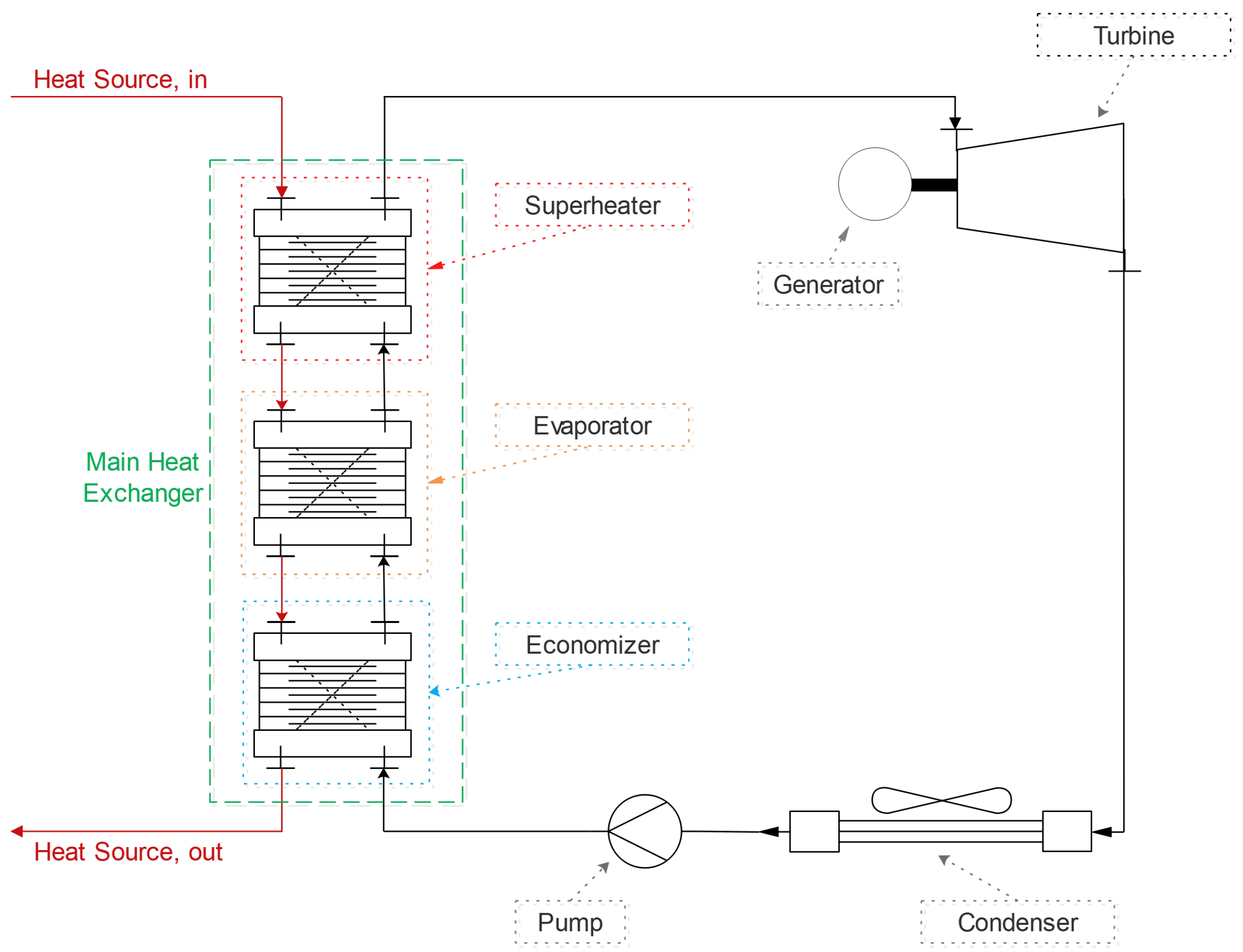
The steam Rankine cycle configuration implemented into the IRC-PD tool is shown in Figure 1. The plant layout is the most simple in order to keep the WHRU cost, weight, and occupied volume as low as possible [26,27]. As a need arising from the fact that the heat source is a waste flux, hence, the SRC design needs to be guided by layout simplicity and, subsequently, cost-effectiveness. Note that, in order to also make available WHRU based on SRC in applications characterized by particular needs (e.g., a gaseous heat source and an area for the WHRU installation far away from the source outlet), the IRC-PD tool can design both the SRC and the thermal loop (using water or oil) in order to decouple the heat source from the WHRU.
The organic Rankine cycle configurations implemented in the IRC-PD tool are the basic and the recuperative configurations, the regenerative and recuperative architecture presented by Branchini et al. [28], the dual pressure and dual fluid layout developed by Shokati et al. [29], and the dual-stage scheme proposed by Meinel et al. [30]. In the aforementioned plant layouts, there is a direct heat exchange between the heat source fluid and the ORC medium, but this is a dangerous way of transferring the heat in case of flammable organic fluids. Therefore, to avoid the risk of flammability that can be occurred in the case of direct contact between the heat source medium and the organic fluid, the IRC-PD tool automatically couples the aforementioned configurations with a thermal loop, which, in turn, adopts water or diathermic oil as working fluid. Specifically, based on plant manufacturers’ experience, the water is used for low temperature heat sources because, usually, it reaches a maximum temperature of 160 °C. The experience also suggests to use the diathermic oil (in the present study Therminol 66 or Therminol VP-1) for medium to high temperature heat source because it can operate at a maximum temperature of 360 °C (Therminol 66) or 400 °C (Therminol VP-1).
Note that the adoption of both water and oil thermal loop can be forced in the IRC-PD tool by the user in the case of specific needs arising from the under-investigation test case. As for the thermal loop, the user can also exclude one or more ORC configurations; as an example, the authors can explore only the basic and the recuperative ORC layouts because the others are much too complex or difficult to be managed for the selected case.
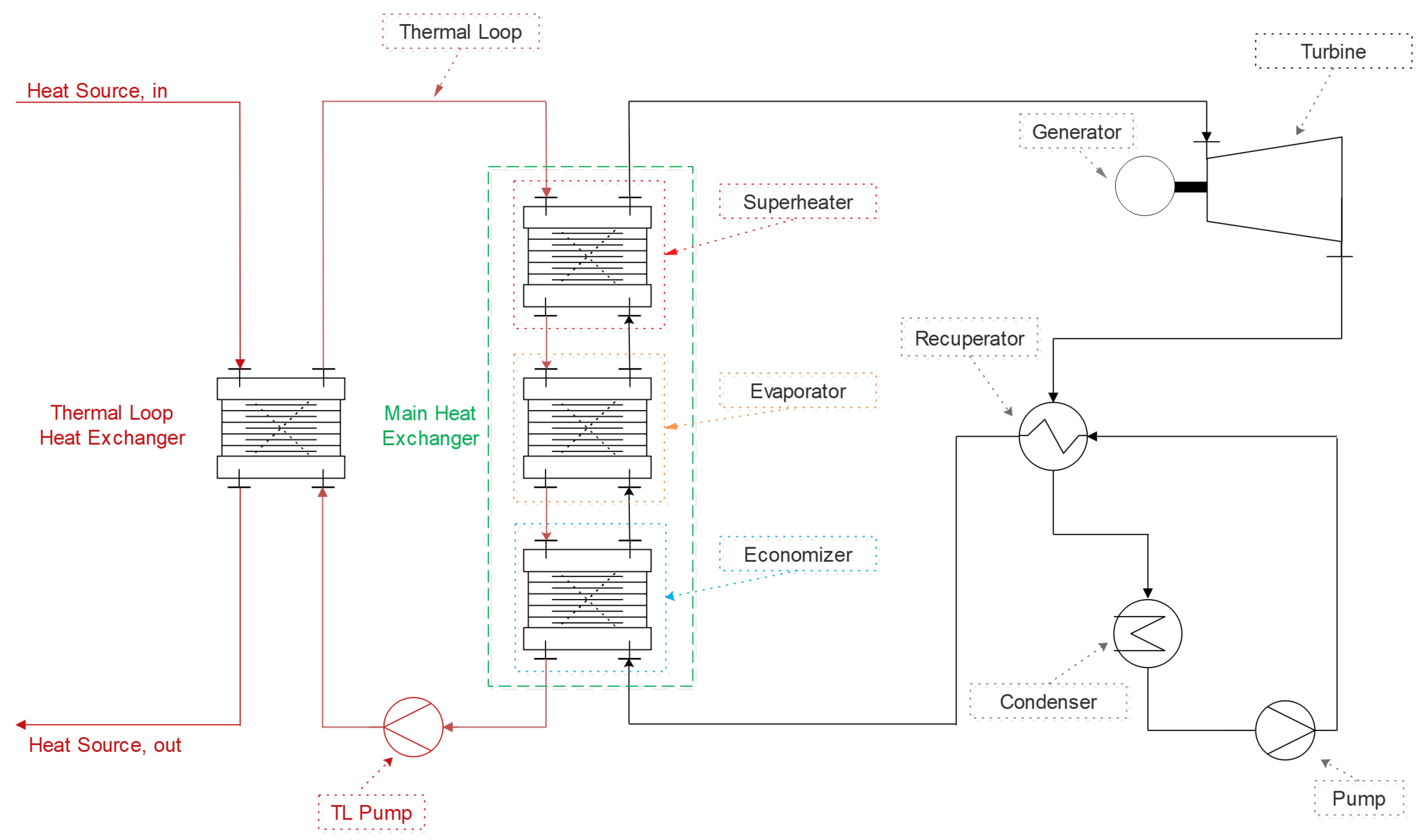
Figure 2 depicts the scheme of a recuperative ORC unit equipped with the thermal loop. The condenser is depicted as a water-cooled one, but, as for SRC unit, the user can select the type between the latter and the air-cooled condenser depicted in Figure 1.
All the proposed ORC layouts can be designed as sub- or trans-critical cycles. The selection of the most appropriate layout and the determination of the necessity of superheating the working fluids are results of the optimization process.
Thanks to the selected way of implementing the IRC-PD tool, it is possible with a unique code to optimize and design ORC units working with (i) low (geothermal, solar, etc.), as well as medium and high, temperature heat sources (exhaust gases released by, e.g., gas turbines, internal combustion engines, industrial processes, etc.); and (ii) heat sources characterized by different nature (e.g., gaseous medium, such as exhaust gases of a boiler or liquid substances, such as the geothermal water).
As extensively discussed in literature, the working fluid of an ORC unit operating with a low or ultra-low temperature heat source is different from the one which needs to be adopted in an ORC linked to a high temperature heat source. To this end, more than 120 pure fluids (HydroCarbons, HydroFluoroCarbons, PerFluoroCarbons, Siloxanes, etc.) and their mixtures are included into the code, thanks to the direct link of the IRC-PD tool with both REFPROP [23] and CoolProp [24] databases. The collection of two databases ensures covering the fluid lack, which can be observed adopting a single source of data.
Regarding the possibility of selecting a mixture as ORC working fluid instead of pure one (see, e.g., References [31,32,33]), it is important to highlight that the IRC-PD tool can (i) use the pre-defined mixture implemented on CoolProp database and (ii) set up the mixture starting from both REFPROP and CoolProp available fluids. To do that avoiding unfeasible composition and time-consuming computations, the method proposed by Venkatarathnam and Timmerhaus [34] is implemented to select the mixture components. Despite the fact that the method was developed for cryogenic refrigerants, Chys et al. [35] suggested its adoption for ORC applications, as well.
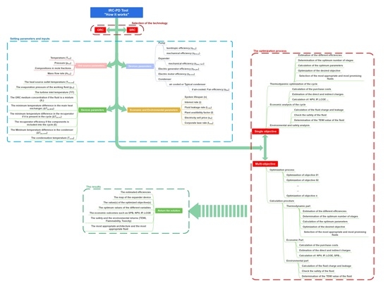
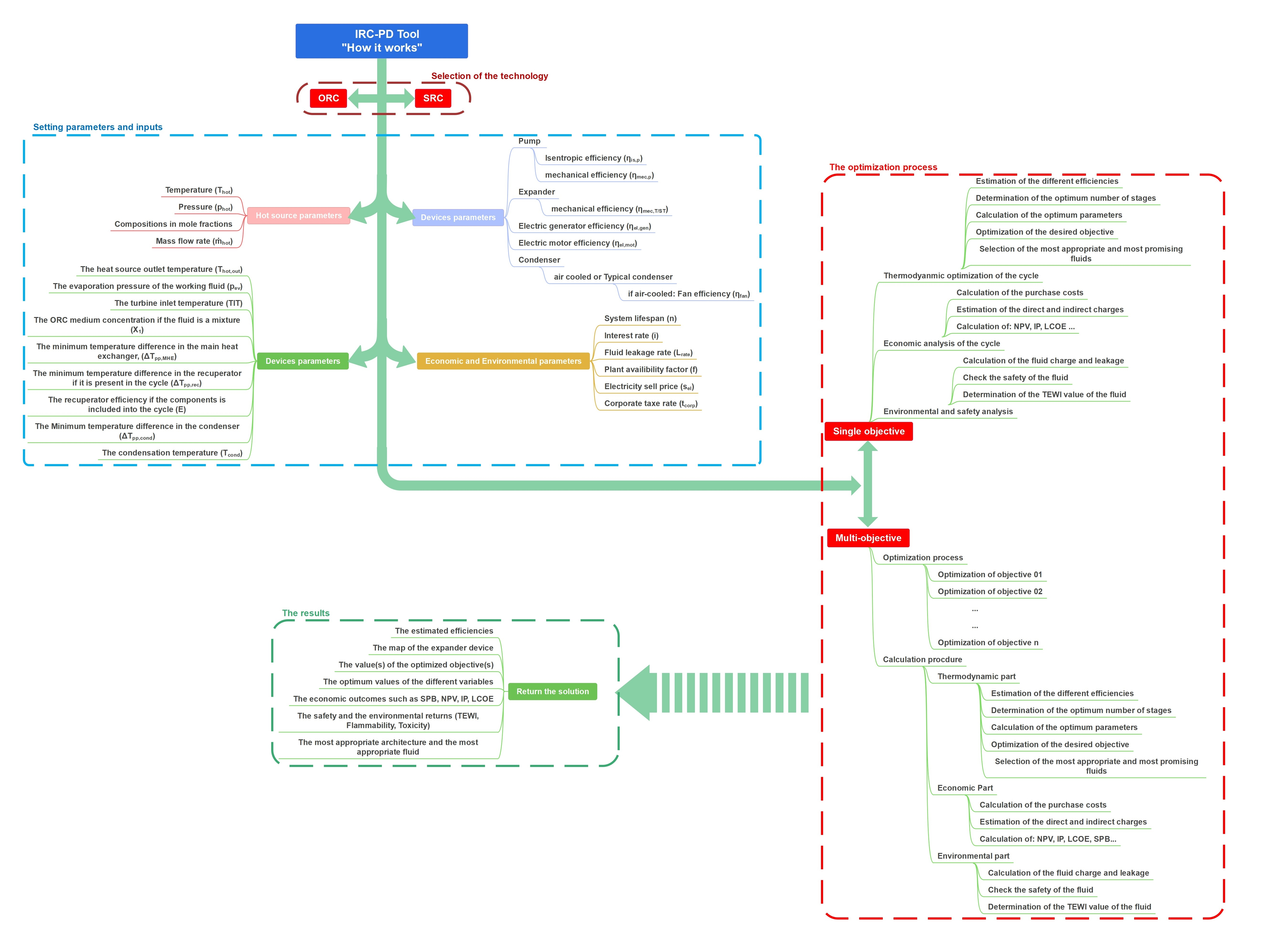
The availability in a unique code of two cycle types (SRC and ORC), different configurations for both cycles (including the thermal loop), and, for the ORC unit, a large set of possible working fluid candidates (including pure fluids and mixtures) are hallmarks of the IRC-PD tool. Despite that fact, these features do not guarantee to cover the entire user’s needs arising from the fact that the tool has to be able to optimize the WHRU independently to the heat source type and thermophysical properties. To this end, the tool was built in such a way that the user can run both single- and multi-objective optimization using several objective functions (e.g., the maximization of the net electric power, the thermal efficiency, the net present value, etc. or the minimization of the simple pay back time, the exergy losses, etc.) requiring only a few parameters as input:
- Heat source:
- −
- Medium;
- −
- Mass flow rate;
- −
- Inlet temperature;
- −
- Inlet pressure.
- Pump:
- −
- Isentropic efficiency;
- −
- Mechanical efficiency.
- Electric motor efficiency;
- Electric generator efficiency;
- Expander mechanical efficiency.
The variables that can be optimized by the IRC-PD tool, for each working fluid, are:
- the heat source outlet temperature, Thot,out;
- the evaporation pressure of the working fluid, pev;
- the turbine inlet temperature, TIT;
- the ORC medium concentration if the fluid is a mixture, X1;
- the minimum temperature difference in the main heat exchanger, ;
- the minimum temperature difference in the recuperator if it is present into the cycle, ;
- the recuperator efficiency if the components is included into the cycle, E;
- the Minimum temperature difference in the condenser, ; and
- the condensation temperature, .
In the case where the thermal loop is adopted, there is also a need to fix the oil or water pump isentropic and mechanical efficiency, while the code also provides, as optimization variables, the oil or water mass flow rate and the returning temperature of such intermediate fluid.
To show how the IRC-PD tool performs the thermodynamic, economic, environmental, and safety analyses, see Section 2.1, Section 2.2 and Section 2.3.
2.1. The Thermodynamic Analysis
For the computation of the thermodynamic points and other SRC and ORC parameters, the equations presented in Appendix A are implemented into the code. Appendix A also lists the fluids available into the code (see Table A1).
Compared to previous code [17,21] and with the aim of making the code able to design both SRC and ORC, several innovative features have been implemented.
Firstly, the main heat exchanger, the recuperator (if present), the condenser, and the thermal loop heat exchanger are discretized into “n” elements, and, for each of them, the tool calculates the thermodynamic states of the fluids in exchange in input as in output. Then, the code checks the pinch point and verifies the constraints violation in each element. This process is necessary as a means to better match the hot fluid profile with the cold one, since the pinch point position is not predefined, a feature which guarantees to design sub- and trans-critical cycle without modifying the code. Obviously, a high number of discretized elements is required, as a means to identify the exact position of the pinch point and avoid its violation. The non-predefined pinch point position and the non-fixed pinch point value in heat exchangers are innovative features implemented in the IRC-PD tool. The tool, in case of mixtures, employs the method suggested by Bell and Ghaly [36] to correct the heat transfer coefficient obtained by Shah [37]. This approach is also used to precisely design both the water- and the air-cooled condenser. The possibility of selecting a particular type of condenser based on water availability in the WHRU installation site or the user needs is an important point of novelty that, to the authors’ best knowledge, is not present in the literature in this kind of optimization tools.
Another novelty introduced into the IRC-PD tool is its ability of providing, as an optimization variable, the efficiency of the single or multi-stage turbine, as well as its preliminary design. In particular, the overall efficiency of the single-stage or the multi-stage steam turbine for the SRC cycle is computed using the correlations and the correction factors presented by Bahadori and Vuthaluru [38], where, in the case of multi-stage steam turbine, the number of stages is computed fixing the maximum specific enthalpy drop to each stage equal to 150 kJ kg−1.
The isentropic efficiency of the single-stage turbine used for the ORC cycle is estimated by employing the method proposed by Macchi and Perdichizzi [39] for axial flow turbine and the one presented by Perdichizzi and Lozza [40] for radial flow machine.
Whilst, in the case of a multi-stage turbine, the isentropic efficiency is determined by employing the method developed by Astolfi et al. [41], in this method, two limits are added to the tool to be able to compute the number of stages, symbolized in the volume ratio and the specific enthalpy drop. The volume ratio in each stage is fixed equal to 4, whereas the specific enthalpy drop is calculated based on the load coefficient (kis) and the mean peripheral speed. The coefficients are, respectively, set equal to 2 and 255 m s−1, as suggested by Astolfi et al. [41] and Martelli et al. [42]. Therefore, the specific enthalpy drop is computed as:
In case the mentioned limits are outstripped, the expansion process is divided into the minimum number of stages that fulfills the previously described conditions. Then, if the number of stages is higher than 3, the value is reset to 3 stages, and the new specific enthalpy drop and the new volume ratio are computed again under the new condition. This change was introduced since some studies mentioned that a number of stages that exceeds 3 does not provide a significant improvement in the turbine’s efficiency but increases the complexity and the costs [43].
So, once the specific enthalpy drop and the volume ratio are determined, the tool computes the size parameter and the specific speed of each stage. Then, it estimates the isentropic efficiency for the turbine, whatever its arrangement, axial or radial, by employing the methods presented by Macchi and Perdichizzi [39] and Perdichizzi and Lozza [40], respectively.
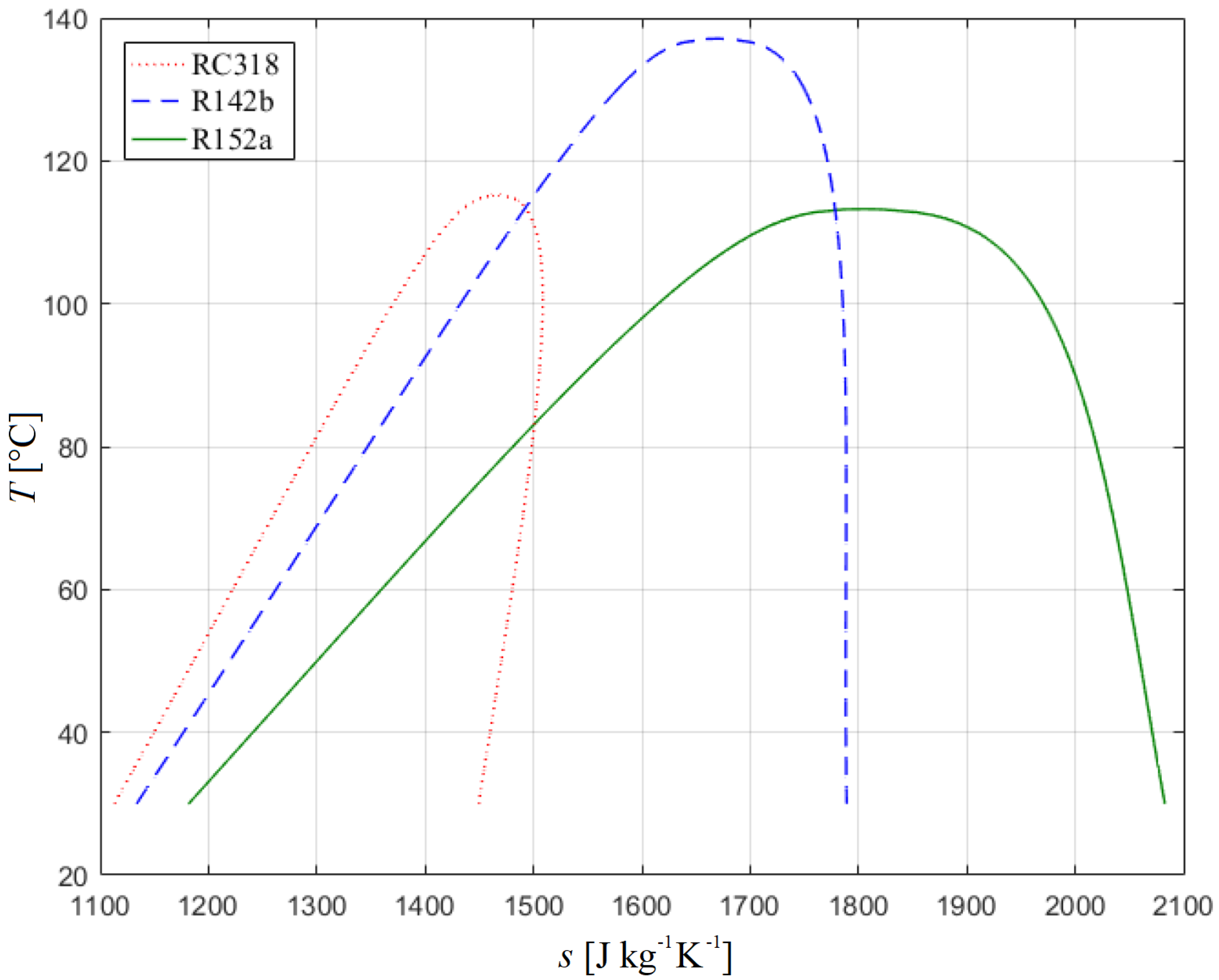
Given the code’s ability to design both SRC and ORC, there is a need to identify the fluid type in order to properly evaluate the need or not of superheating the fluid itself. To this end, the IRC-PD tool classifies the fluids according to their vapor saturation line into three categories: dry, isentropic, or wet, by employing the method proposed by Liu et al. [44]. The method consists of the derivation of the specific entropy by the temperature:
The fluid is dry when > 0, while it is isentropic and wet in the case of 0 and < 0, respectively.
For the prediction of the slope, Liu et al. [44] simplified the equation using the relations of the ideal gases:
where TH is the standard boiling point, hH is the evaporation specific enthalpy change, n is a coefficient generally varying in the range between 0.375 and 0.380, and cp is the specific heat, while TrH is defined as:
where Tc is the critical temperature, and TH is, again, the standard boiling point.
For the sake of clarity, Figure 3 depicts the vapor saturation line of the three different types of fluids.
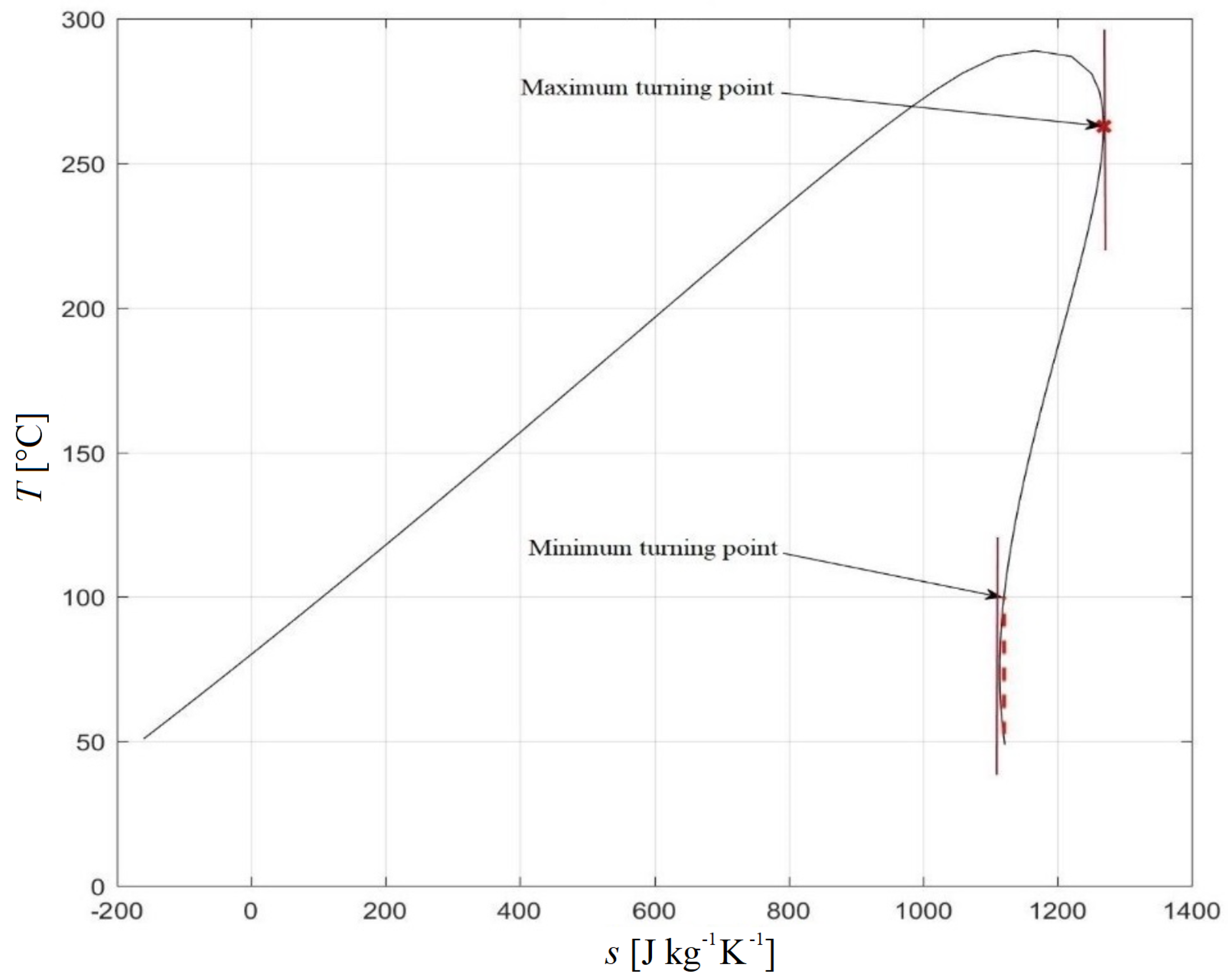
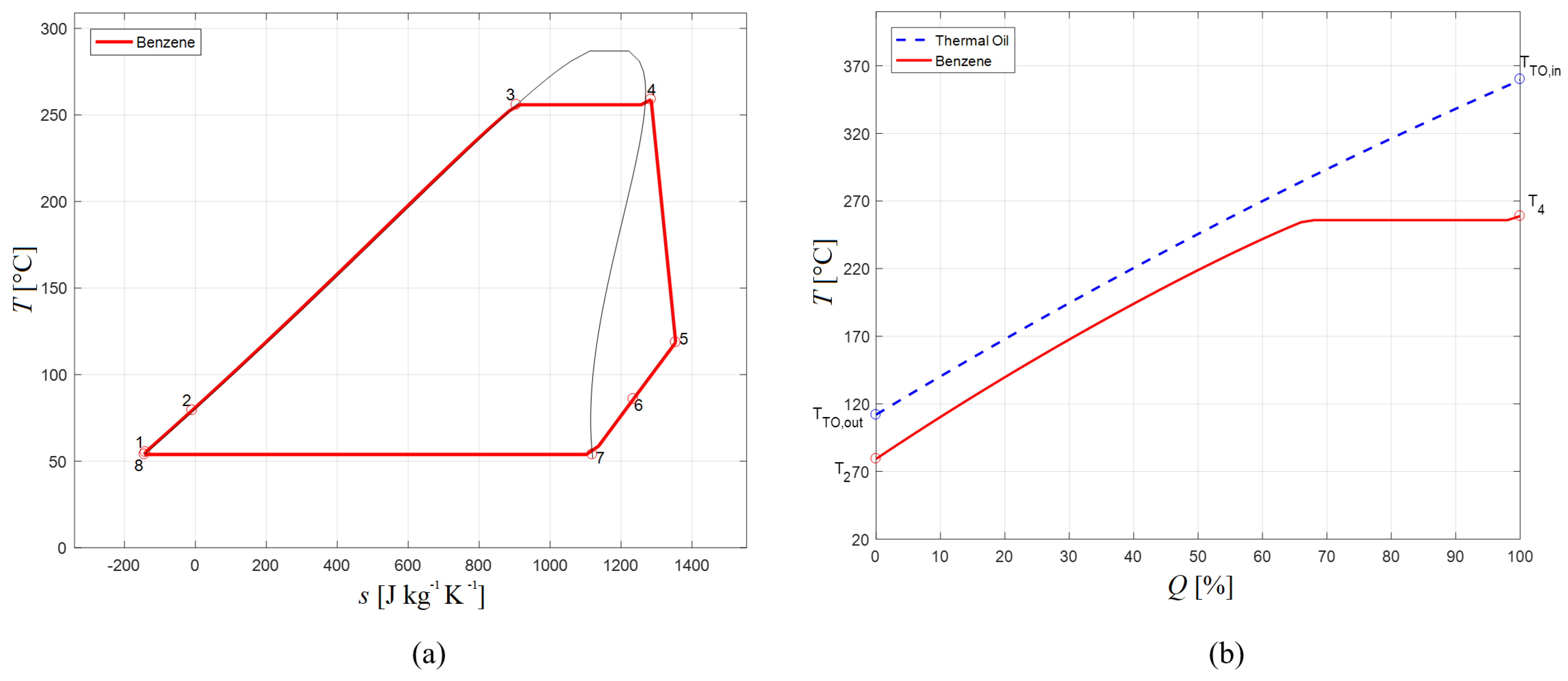
During the design of both SRC and ORC, there is also a need for checking the vapor quality at the end of the expansion process to avoid the turbine’s blade erosion, an aspect which is directly linked to the need for superheating the fluid. To manage this issue, the IRC-PD tool adopts the approach proposed by Wang et al. [45], which introduces the concept of the turning point for the isentropic and dry fluids. This point corresponds with the maximum value of the fluid evaporation temperature that can safely enter the turbine without the need for superheating, since all values below this limit are acceptable, as opposed to higher values, for which superheating is mandatory. However, Wang et al. [45] do not consider the behavior of some fluids, which may show a minimum turning point, as well, where their saturation line takes a reverse path in some points, e.g., Benzene. Therefore, to better describe the behavior of these particular fluids and avoid the turbine’s blade erosion caused by a reverse path of the saturation line, the authors introduce the concept of the minimum turning point and combined it with the maximum one defined by Wang et al. [45]. This constitutes an important point of novelty that no one previously adopted into an ORC optimization tool. For the sake of clarity, the two points are depicted in Figure 4.
The check is performed employing Equation (5), where the temperature T is equal to the turning point Ttn in the saturated vapor () line:
In the event that the evaporation temperature is higher than the maximum or below the minimum turning point, the tool performs another check as a way to guarantee that there is no liquid formation during the expansion process. In case where the liquid is present, the tool runs the simulation again at another evaporation temperature.
The aforementioned distinctive traits of the IRC-PD tool are coupled with several checks that guarantee to avoid pinch point violations in the heat exchangers, the presence of liquid at the turbine inlet, a low value of steam quality at the turbine outlet, and, if the recuperator is part of the layout, guarantee that the evaporation process does not take place in this device. The IRC-PD tool also provides a warning if the organic fluid has been banned or if it is phasing out. In addition, in the tool, there is another set of checks and warnings devoted to the detection of possible numerical issues that can occur during the evaluation of the fluid thermodynamic properties, especially during the acquisition of values from REFPROP and CoolProp databases.
In the case of a single objective optimization aiming to maximize, e.g., the net output power or the cycle efficiency, at the end of the optimization process, the user can decide whether or not to perform the exergetic, economic, and environmental analyses. For a detailed description of the exergetic analysis, the reader can refer to Pezzuolo et al. [21], while the economic and environmental analyses descriptions are given in Section 2.2 and Section 2.3, respectively. The latter is another distinctive trait of the IRC-PD tool because, to the authors’ best knowledge, this kind of analysis has not been included in previously presented optimization codes.
In the case of a multi-objective optimization, the code handles the thermodynamic, exergetic, economic, and environmental analysis based on the selected optimization goals.
To the authors’ knowledge, the implemented features and the adopted structure of the IRC-PD tool guarantee higher optimization flexibility and lower computation time compared to other optimization tools, such as the ORC-PD one (the latter has also been developed by the University of Padova research group [17,21]).
2.2. Economic Analysis
To estimate the purchase costs of the different devices and carry out a preliminary economic analysis, several correlations and equations are included in the IRC-PD tool in order to cover the equipment size range from small to large. The selection of the equations is performed by the code, depending on: (i) the equipment size, (ii) the case study, and (iii) the desired application.
The economic evaluation is computed adopting the technique of preliminary cost estimation for chemical plants, named Module Costing Method (MCT). This technique guarantees to estimate the purchase costs considering both direct and indirect charges, according to basic estimated costs.
The Main Heat Exchanger (MHE), the recuperator, the water-cooled condenser, and the heat exchanger in the thermal loop can be of different sizes (as said, ranging from small to large), depending on the case study. Thus, the purchase costs of these heat exchangers are estimated by the equation presented in Reference [46] for small-scale WHRUs (heat transfer area lower than 80 m2), while, in the case of heat transfer area ranging between 80 and 4000 m2, the code adopts the equation proposed by Smith [47].
The purchase costs of the single-stage turbine, of the pumps adopted in the SRC, the ORC, and the thermal loop, as well as the one of the air cooled condenser, are also computed based on the equations proposed by Turton et al. [46], while the approach suggested by Smith [47] is employed for the fans, including their electric motors. The cost of the electric generator is predicted using the equation developed by Toffolo et al. [48].
For the computation of the purchase cost of the ORC multi-stage turbine, the equation proposed by Astolfi et al. [41] is employed, while the equation suggested by Manesh et al. [49] is used in the case of a steam multi-stage turbine.
In a nutshell, the general form of the purchase cost equation for heat exchangers with an area ranging from 80 m2 to 4000 m2, the fan, including its electric motors, and the electric generator is:
where is the purchased equipment cost, CB is the base cost of the equipment, M is a constant peculiar to each device, and N is the capacity or the size parameter of the equipment, while QB is a coefficient.
In contrast, the equation used for other devices, including the heat exchangers with an area lower than 80 m2, can be expressed as:
where N is the capacity or the size parameter of the equipment, and K1, K2, and K3 are correction factors which depend on each piece of equipment.
To compute the bare module cost, CBM, several correction factors, FBM, are needed. Their values are selected based on the system’s pressure, the material selected to build the device, and, in some cases, the device’s operating temperature. So, the bare module cost general equation for the different devices can be written as:
where, for the heat exchangers and the fan, including its electric motor, FBM is given as:
where FM is the material correction factor, FP is the pressure correction factor, and FT is the temperature correction factor. These correction factors can be determined using the indexes listed in Reference [47].
The remaining devices’ bare module correction factors FBM are computed as suggested by Turton et al. [46]:
where the pressure correction factor, FP, can be computed as:
C1, C2, and C3 are correction factors peculiar to each device. Conversely, for the electric motor and the electric generator, the FBM is directly given in Reference [46].
The purchase cost equation of the multi-stage expander adopted in the ORC cycle is derived from Reference [41], where the cost is a function of the number of stages n, and the last stage size parameter SPLS:
where C0 = 1230 k€, n0 = 2, and SP0 = 0.18 m.
In contrast, the cost of the steam turbine, CST, is calculated employing the steam mass flow rate () and the turbine’s inlet pressure (pev), as suggested by Manesh et al. [49]. The purchase cost is expressed in M$, and it is computed as:
In addition, the chemical engineering plant cost index (CEPCI 2019: 607.5) is adopted to calculate the “new purchase costs” for the different devices. Therefore, the new bare module cost of each equipment is computed in accordance with the equation proposed by Zhang et al. [50].
Then, the total cost of the cycle, CBMT, is calculated as:
where CBMi represents the investment of each device.
In accordance with Pezzuolo et al. [21], the cost of the site, Csite, is determined by multiplying the total cycle cost by 1.4:
while the operation and maintenance cost, CO&M, is calculated by multiplying the site cost by 0.02:
The annual benefits deriving from the electricity sale (also named cash flow), CF, can be estimated as:
where
tcorp is the corporate tax rate, Sannual is the annual income from the sale of electricity, f is the operational factor, sE is the price of electricity, and Eel is the annual production of electricity.
The net present value, NPV, therefore, is computed as:
where the capital recovery factor, RF, is given as:
where i is the annual interest rate and n is the expected life. Thus, the NPV can be rewritten as:
The profitability index, IP, is calculated by dividing the net present value by the total costs, including the site one:
while the Levelized Cost of Energy, LCOE, is defined as the cost associated with each unit of produced electrical energy, and it is calculated as:
Finally, the simple payback, SPB, which is the ratio between the total costs and the annual benefits, can be expressed as:
More details about parameters and assumption adopted in the economic analysis can be found in Appendix B.
2.3. Environmental and Safety Analysis
The environmental impact and the safety conditions are considered as a key point during the selection of suitable fluids. In fact, the fluids should have low toxicity and flammability to avoid the need for site protection measures.
So, as a way to assess the safety of the fluids, the concept introduced by ASHRAE standard 34 [51] is employed, where the tool can classify the working fluid based on its safety level in accordance with the classes defined in Table 1.
Then, from an environmental point of view, the value of Ozone Depletion Potential (ODP) and Global Warming Potential (GWP) need to be in the controlled zone as specified by the international treaties and regulations, such as the Montreal protocol for ODP [52] and the EU Directive 2006/40 for GWP [53]. For this purpose, the Total Equivalent Warming Impact (TEWI) method is adopted and implemented in the tool for environmental analysis.
The TEWI general formula for the estimation of the environmental impacts is defined in accordance with Gullo et al. [54]:
where TEWIdirect represents the direct emissions of greenhouse gases, including the leakages of refrigerant into the atmosphere [55]. The latter can be calculated employing the GWP of the fluid:
where L, M, , and n are the fluid leakage (kg year−1), the refrigerant charge (kg), the recycling factor (%), and the system lifetime (year).
The TEWIindirect refers to the CO2 emissions due to the generation of the consumed electricity [55,56], and it is computed as:
where Ea, , and n are the consumed energy (kWh), the carbon dioxide emission factor (kgCO2eq kWh−1), and the system lifespan (year).
To perform the environmental and safety analysis, the IRC-PD tool is linked to a separated database that contains the different environmental and safety parameters for the different fluids, as well as information regarding the organic fluid phase out. These parameters are derived from ASHRAE 34 or predicted from material safety data sheets of the fluids which are available in the literature (see, e.g., Reference [57]). In this way, it is possible to rank the ORC optimize configurations based on their safety and environmental friendliness.
Note that, for the refrigerant charge, the method suggested by Collings et al. [58] is implemented in the tool to estimate its value, where it depends on the energy transferred through a heat exchanger and the power extracted through the turbine.
3. The Tool Validation Procedure
The validation process of a new tool is a fundamental step, especially in the case of highly complex tools, such as the IRC-PD one. To this purpose, the code needs to be tested using different plant configurations and heat sources as suggested by, e.g., Pezzuolo et al. [21], where several cases are taken from the literature and use as reference for the comparison with the developed tool.
For testing the ORC basic configuration, the IRC-PD tool was set up with the specifications presented by Vaja and Gambarotta [59]. Three fluids have been screened, the first one without superheating, and the rest with the superheating. For the first one, Benzene, the results obtained by the IRC-PD tool exhibit a deviation of about 3% in terms of net power output, while the maximum deviation is around 3.8% if the turbine inlet volumetric flow is considered. The other parameters show a deviation lower than 1%.
The results obtained with the IRC-PD tool for the fluids R11 and R134a, and the same conditions reported by Vaja and Gambarotta [59], denote a deviation of about 2.5% in the net power output for R11, and lower than 1.7% for R134a. For the mass flow rate of the working fluid, the adoption of R11 showed a deviation less than 2.6%, while a deviation less than 1.5% is observed in the case of R134a. The other parameters, as previously, denote a deviation lower than 1%. A clear overview of the obtained results are given in Table 2. The small deviations in the results can be mainly attributable to a not precise estimation of the heat source mass flow rate. In fact, this value is not listed in ref. [59]; thus, the authors estimate it.
To validate the recuperative configuration, the authors selected the case study presented by Chys et al. [35], in which five pure fluids are considered as possible working medium candidates. The comparison between the reference case and the IRC-PD tool results are given in Table 3. The deviations analysis clearly pointed out that the discrepancy are in the 0.34–1.25% for the generated power, while, for the mass flow rate and the efficiency, the maximum deviation reaches 1.79% and 1.06%, respectively. As in the case of the basic configuration, the recuperative one can also be considered validated, given that the IRC-PD tool results are in line with the one reported in the selected reference.
The IRC-PD validation also included the configurations adopting the thermal oil loop as a medium to transfer the heat from the source to the ORC. In this case, the reference work is the one presented by Liu et al. [60], where the adopted oil is the so-called Dowtherm Q. As for the other validation scenarios, the results revealed that the highest deviation is observed in the working fluid’s mass flow rates and the cycle efficiency (1.6% and 1.5%, respectively), while the other parameters present a deviations below 1%, as listed in Table 4.
With the aim of exploring the cycle’s performance improvements and the computational cost of adopting a detailed method to predict the turbine’s performance and its design, the authors constrained the IRC-PD tool as the ORC-PD one and considered the case presented by Benato and Macor [17]. The simulation outcomes are given in Table 5.
The results show that the adoption of a multi-stage turbine instead of a single-stage one guarantees higher isentropic efficiency of the ORC turbine, thus contributing to higher net output power. In fact, the cycle working with Toluene and adopting a multi-stage turbine generates a net output power 23% higher than the same cycle mounting a single-stage turbine [17]. Similarly, adopting a multi-stage turbine instead of a single one (as given in Ref. [17]) guarantees reaching a net power output 15% and 14% higher in the case of Benzene and Acetone, as well. In terms of computational efforts, the introduced features do not drastically affect the speed. In fact, the computational time only increases 2%. These outcomes clearly show the importance of adopting a detailed model for the turbine at the optimization stage, as well, because this is the only way that it is possible to properly predict the generated electricity and the cycle performance, as well as provide a preliminary design of the machine.
Finally, the steam cycle configuration was tested replicating the plant setup presented by Nord et al. [26]. As previously, the simulation outcomes derived with the IRC-PD tool are perfectly in line with the one reported in the reference because the highest observed deviation is smaller than 2%.
In a nutshell, considering the obtained findings and the large variety of performed tests, it is possible to claim that the code is able to replicate the results reported in the references; thus, it can considered validated.
4. Case Study and Optimization Settings
To test the code ability of selecting the most performing WHRU, the authors chose an internal combustion engine fed by bio-gas as the test case. This choice was driven by the need for the Algerian’s research group to evaluate the benefits of adding a WHR to upcoming bio-gas installations, while the Italian’s researchers want to evaluate the ICE’s recovery potential considering both SRC and ORC configurations.
The selected ICE is an Italian power system installed on a bio-gas plant located in Northern Italy, as well as the power unit that will be installed on future Algerian bio-gas plants. The bio-gas ICE is a GE power unit [61], and the nameplate data is listed in Table 6.
The plant adopts a standard and well-established layout made up of a reception tank, two primary fermenters and two secondary fermenters, a gas holder, an overflow tank, and the bio-gas engine. The ICE waste heat recovery can be done only in the exhaust gases stage because of the heat of the cooling water and lube oil already recovered and used to maintain the digesters at a temperature of 42–44 °C.
The data used to design the WHRUs are not the nameplate ones but the results of an experimental campaign that demonstrated a large mismatch between the measured and the nameplate exhaust gases mass flow rate and temperature [17]. In particular, the measured mass flow rate and temperature of the flue gases are 6477 kg h−1 and 503 °C, while the exhaust gas compositions on mole fractions are: CO2 (6%), N2 (74%), O2 (14%), H2O (5%), and Argon (1%). More details about the experimental campaign can be found in ref. [17].
The use of these data guarantees selection and design of the WHRU based on real data, as well as comparison of the obtained findings with the ones presented by Benato and Macor [17], where a less advanced optimization tool was adopted.
Note that, despite the fact that the literature presents a large number of innovative technologies to recover the ICE’s waste heat (see, e.g., Kalina cycle [62] and super-critical CO2 cycle [63]), acceptable performance improvements and techno-economic feasibility are today reachable only with WHRUs based on the steam and the organic Rankine cycle.
As an example, Yu et al. [64] proposed to recover the exhaust gases heat content of a heavy-duty diesel engine by means of a cascaded dual-loop WHRU composed by an SRC and an ORC. The results revealed that the 101.5 kW of waste heat can be generated up to 12.7 kW, ensuring a 5.6% power increment of the system. Similarly, Liu et al. [65] analyzed the possibility of recovering the waste heat of a 14-cylinders marine engine using a WHRU which combines an SRC and the dual pressure ORC. They also compared the performance of this configuration with the one reachable with a WHRu composed by an SRC or a dual pressure ORC. The results outline that combining the SRC and the dual pressure ORC guarantees a fuel saving of 9355 tons per year and an improvement of the system’s efficiency of 4.42%. Contrary, the SRC and the ORC alone guarantee a higher simplicity but lower thermal efficiency improvements, 2.68% and 3.42%, respectively. Andreasen et al. [66] studied how to improve the performance of a 23-MW two-stroke MAN diesel engine working at a load variable between 25 and 100% of the design power. They proposed to adopt a dual pressure steam Rankine cycle or an ORC. The results of the simulations indicate that the SRC unit is able to improve the power of 18%, while the ORC unit adopting MM produces 33% more power.
In contrast to previous studies, Yang et al. [67], Wang et al. [68], and Song and Gu [69] proposed to recover the diesel engine waste heat by means of a dual loop ORC, while Shu et al. [70] evaluated the system performance improvements reachable with a recuperative ORC layout using a mixture as working fluid. In particular, the use of a mixture of Benzene and R11 can increase the system thermal efficiency up to 16.7%.
As said, several works available in literature study the diesel ICE’s waste heat recovery using ORC, especially for marine applications (see, e.g., References [59,71,72,73,74,75]), while only a few are focused on engines fed by bio-gas.
Schulz et al. [76] and Kane et al. [77] were among the first to suggest the use of the ORC technology to improve the agricultural bio-gas plants performance and to apply the ORC to these engines. In particular, Kane et al. [77] investigated the use of an ORC unit for waste heat recovery from the cooling jacket of a 200 kWe bio-gas ICE. They found that the ORC can reach an efficiency up to 7%.
In addition, Meinel et al. [30] explored the benefits of adding an ORC to a bio-gas ICE. However, in their investigations, an innovative two-stage ORC configuration was proposed and the best working fluid selected among 4 media. The ORC heat source is the constituted by the exhaust gases at 490 °C and 1 bar. The outcomes of the study indicate that the two-stage layout without the recuperator boosts the performance of wet and isentropic fluids, while the one with the recuperator is more appropriate for dry fluids. In terms of performance, the two-stage non-recuperative configuration operating with isentropic fluids improves the thermodynamic efficiency up to 2.25% compared to conventional ORC layout, while the recuperative one operated with dry fluids reaches efficiency improvement up to 2.68% compared to standard ORC. Contrary to Meinel et al. [30], Dumont et al. [78] and Koç et al. [79] proposed to improve the bio-gas ICE performance adopting standard configurations: a non-recuperative ORC layout and a regenerative one, respectively. Dumont et al. [78] performed a thermo-economic optimization with the aim of defining the architecture, the working fluid, and the plant components, while Koç et al. [79], after a parametric optimization, carried out an exergy analysis. In Reference [78], the results indicate that R1233zd(E), R245fa, and Ethanol guarantee higher electricity production compared to R134a and R1234yf, but they require higher investments, while, in Reference [79], the authors observed that the higher exergy destruction is in the evaporator. However, the overall thermal and exergetic efficiency are 19.17% and 32.41% for the sub-critical recuperative ORC layout, while they become 18.50% and 31.67% for the super-critical unit. This is not a marginal increment, considering that the sub- and super-critical non-recuperative ORC configuration can reach thermal and exergetic efficiency equal to 15.51% and 27.20% and 15.93% and 27.76%, respectively.
Finally, Saravia et al. [80] and Uusitalo et al. [81] proposed to retrofit the bio-gas ICE with an ORC to reduce engine’s fuel consumption and GHG emissions, respectively. In the first case, an ORC was added to a 6 MWel in-operation ICE fed with landfill bio-gas; a system improvement that guarantees higher overall power production by recovering 5–10% of the fuel energy content. In the second case, using the LCA approach, Uusitalo et al. [81] evaluated the environmental benefits in terms of GHG emissions reduction introduced with the ORC unit. They observed that adding the ORC guarantees a GHG emissions reduction in the range 280–820 ton of CO2,eq, depending on the type of substituted electricity, while the impact of the ORC and its working fluid is only the 0.1% of the total bio-gas ICE power plant GHG emissions.
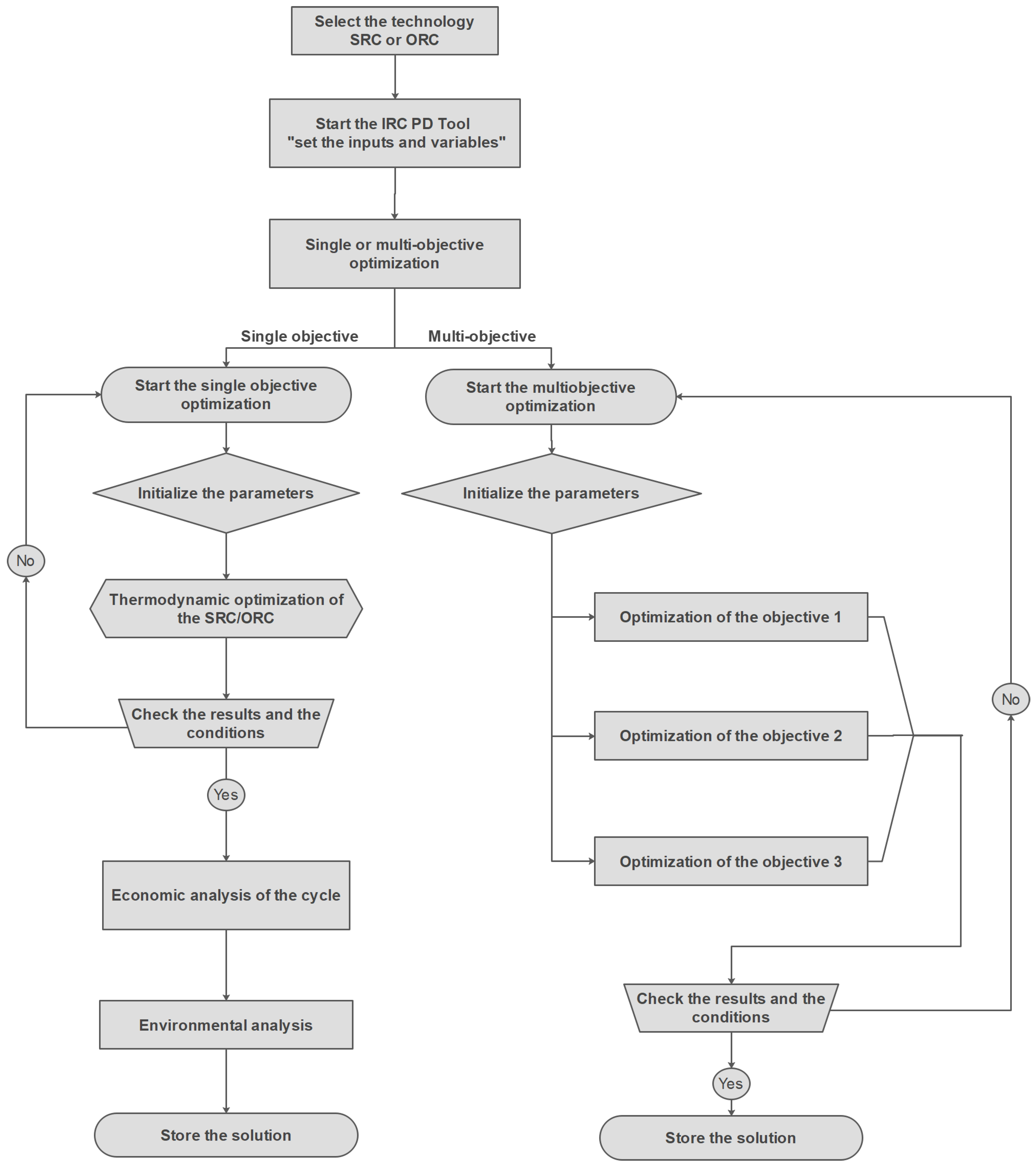
Starting from the literature analysis, it is clear that it is not convenient to study all the possible configurations of the ORC cycle because some of them are characterized by high complexity and costs. In addition, the use of mixtures as working fluids is not convenient (also see Benato and Macor [17]), but the authors set the IRC-PD tool free to explore all the possible configurations and the use of pure, as well as mixtures, as working fluid to be sure that the code excludes these not-performing and less cost-effective configurations and fluids. For the entire set of WHRUs, the adoption of the water and the oil thermal loop is explored, as well as configurations in which the ICE’s exhaust and the working fluid directly exchange the heat. Again, considering the motivation of the work and, in particular, a need to maximize the waste heat recovery, the authors performed a single-objective optimization aiming to maximize the net output power of the WHRU, followed by an economic and environmental analysis. For the sake of clarity, the optimization steps are summarized in Figure A2 (Appendix A), and ORC of the upper and lower bound of the optimized variables is listed in Table 7.
The minimum and the maximum evaporation pressure for the SRC cycle are fixed equal to 15 bar and 40 bar in accordance with the specifications provided by Nord et al. [26].
The maximum pressure, pmax, of the ORC cycle is assumed to be the minimum between the critical pressure, pcrit, and 35 bar.
The selection of this value guarantees reasonable pumping conditions as given by Marcuccilli and Zouaghi [82], as well as reduces the material expenses and improves the plant safety, as underlined by Javanshir et al. [83]. Therefore, the adoption of a pressure lower than 35 bar avoids the need for very expensive pipes, heat exchangers, etc., as well as control and management systems.
On the other side, from the thermophysical point of view, the fluid must have adequate chemical stability in the desired temperature ranges and should have good compatibility with the material in contact with, as the organic fluids prove chemical deterioration and decomposition at high temperature, as pointed out in References [35,84]. To this end, the maximum temperature of the cycle, TITmax, is selected as the minimum between:
where Thot,in is the temperature of the fluid entering the ORC main heat exchanger (MHE), and Tpp,MHE is the minimum temperature difference in the MHE, while Tdecomposition is the organic fluid decomposition temperature.
When a thermal loop is adopted, the user can select the oil type among Therminol VP-1, Therminol 66, and Dowtherm Q. In the analyzed case, the authors’ choice fell on Therminol VP-1 due to its high safety level and stability, no toxicity, and availability at an acceptable price. The oil inlet temperature (Toil,in) is assumed as follows:
where Tmax,bulk represents the maximum operating temperature of the thermal oil without risk of thermal degradation, while Thot,in is, in this case, the temperature of the hot source at the inlet section of the thermal loop heat exchanger. In the case of Therminol VP-1, TBulk is equal to 400 °C.
In regard to the setting of the water loop inlet and outlet temperatures, the authors fix them equal to 160 °C and 140 °C, respectively, a choice driven by the manufacturers’ experience which prescribe to limit the water pressure in the thermal loop and, consequently, the cost of the devices that made up the loop itself.
The different parameters assumed for the genetic algorithm set up are:
- Population size: 500;
- Generation size: 350;
- Crossover Fraction: 0.8;
- Migration Fraction: 0.2.
These assumed values are checked in term of computational time and results accuracy, and they confirmed that adopting higher values for both population and generation (e.g., 700 instead of 500 in population and 500 instead of 350 in generation) do not provide more accurate results but only increases the computational time of up to 30%. For the same reasons, the number of elements in which the heat exchangers have been discretized is assumed equal to 50.
To perform the economic and environmental analysis, the authors assumed a WHRU lifespan equal to 15 years, while the value of the fluid leakage (Lrate) in the ORC and of the recycling factor () is considered equal to 0.02 and 0.8, as prescribed by Gerber and Maréchal [85].
5. Results and Discussion
In this work, the authors perform an optimization aimed at finding the most appropriate technology between SRC and ORC cycles for the selected case study, besides the determination of the most suitable plant configuration and working fluid that guarantees the maximization of the net output power. Concerning the economic analysis of the optimized solutions, it is important to point out that it is difficult to perform it in terms of net present value or simple pay back due to the need for estimating the electricity selling price, a difficult task considering the uncertainties linked to support schemes establish by Governments. So, the authors do not perform an economic analysis but only compute the investment costs of the WHRU.
The tool is set in such a way that, at the end of the optimization process, it provides a set of plots where, for each safety category, the 3 best working fluids that guarantee the maximization of the net output power are shown versus the cost of the WHR unit.
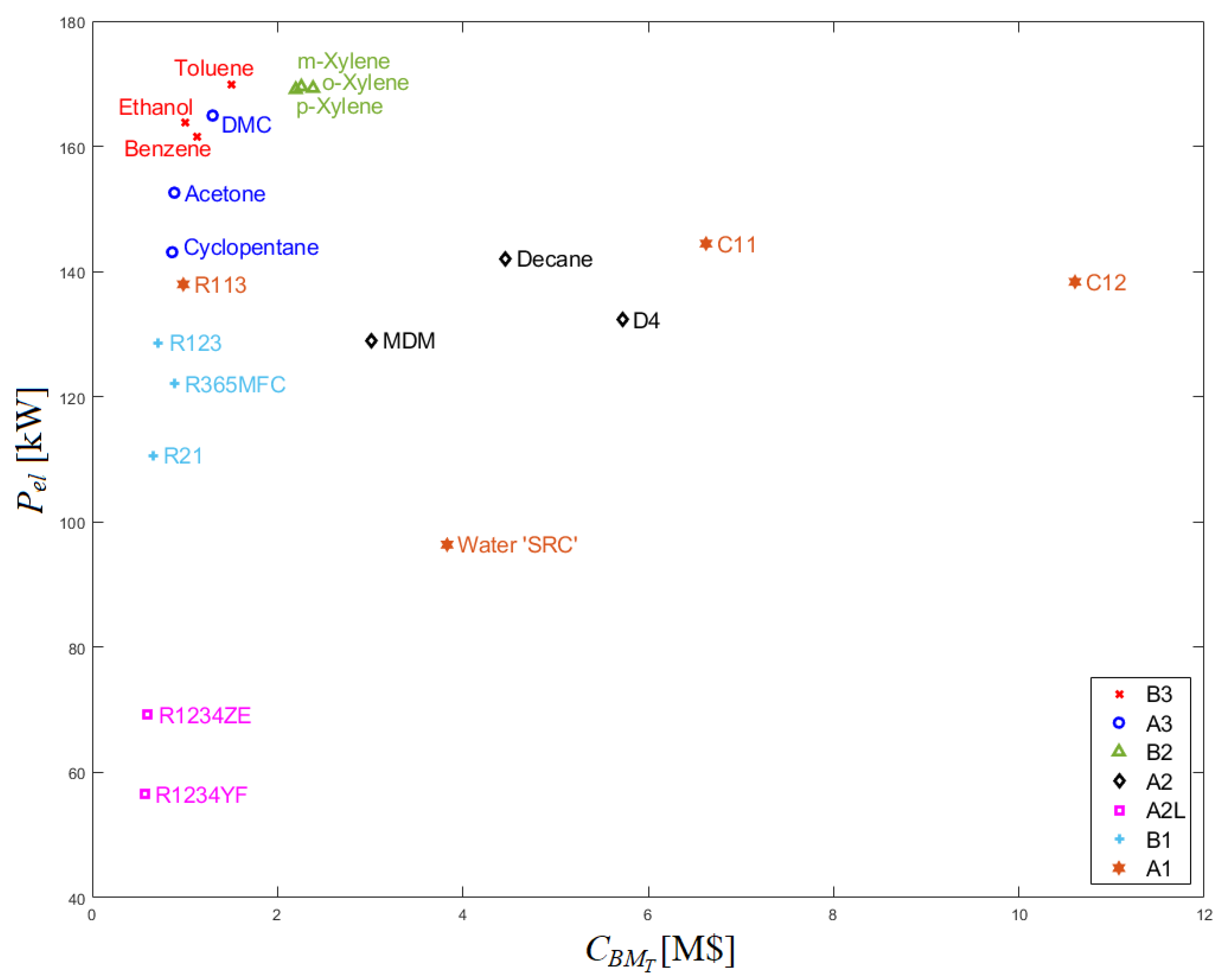
The picture is given for the case with no thermal loop (see Figure 5), as well as for the water and oil thermal loop (see Figure 6 and Figure 7, respectively).
For the sake of clarity, the authors list the results obtained for the SRC when the heat is exchanged directly between the ICE’s exhaust and the cycle (see Table A4), as well as in the case of adopting a water and an oil thermal loop (see Table A5 and Table A6, respectively). Similarly, Table A7 lists the optimization findings in the case of the ORC without thermal loop, while Table A8 and Table A9 report the results of the optimizations when a water and an oil loop is adopted. For compactness, only the first five fluids are listed for each plant configuration. The cost analysis of the different ORC arrangements is given in Table A10, Table A11 and Table A12.
Analyzing the results, it is clear that neither the mixtures nor the regenerative and recuperative, the dual pressure, the dual fluids, and the dual stage are appropriate architectures for the analyzed test case. Additionally, the SRC also does not guarantee acceptable performance compared to ORCs employing pure fluids and a recuperative configuration.
The SRC which guarantees the highest performance (96.37 kW) exchanges directly with the ICE exhaust gases and adopts a multi-stage steam turbine with 7 stages and an isentropic efficiency of 52.8%. The latter is an estimated value perfectly in line with the one expected by the steam turbine manufacturer that collaborates with the authors and the available in literature (see, e.g., Reference [86]). In contrast, the cycle has an optimal evaporation pressure of 19.22 bar, a condensation pressure of 0.15 bar, and a thermal efficiency of 13.96% as listed in Table A4. In addition, the plant is characterized by unfeasible cost per kWel (41 k$ per kWel) because the plant cost reaches the 3.83 M$. It is also important to note that the use of a water or an oil thermal loop drastically reduces the waste heat recovery and increases the plant costs compared to a direct exchange layout (see Table A5 and Table A6). In addition, because water is a non-flammable and non-toxic fluid, there is no safety reason that justifies the adoption of a thermal loop. Finally, it is important to remark that the authors expected that the steam cycle was not a feasible solution for the selected test case due to the small amount of available heat.
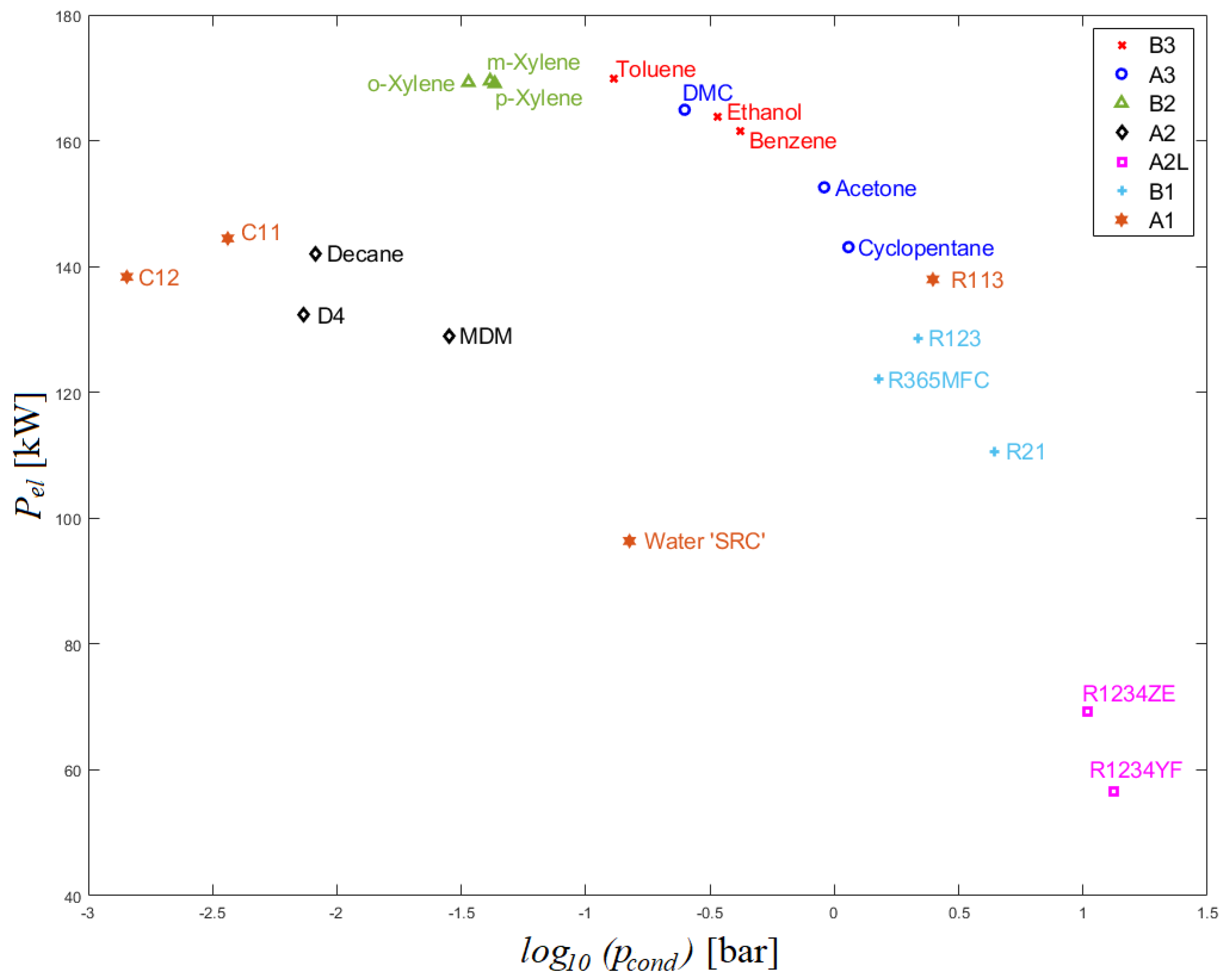
Focusing on the ORC solutions, it is clear that the best performance in terms of net power maximization is guaranteed by a direct exchange between the ICE exhaust and the ORC working fluid. In particular, as shown in Figure 5, the highest performance is reached with Toluene (169.89 kW), followed by M-xylene and O-xylene with 169.50 kW and 169.27 kW (see Table A7 for more details). However, Toluene is a fluid belonging to category B3 (high toxicity and flammability); thus, for safety reasons, it is not convenient to build a plant in which a high toxic and flammable fluid exchange the heat directly with ICE exhaust. Therefore, the use of such fluid is excluded.
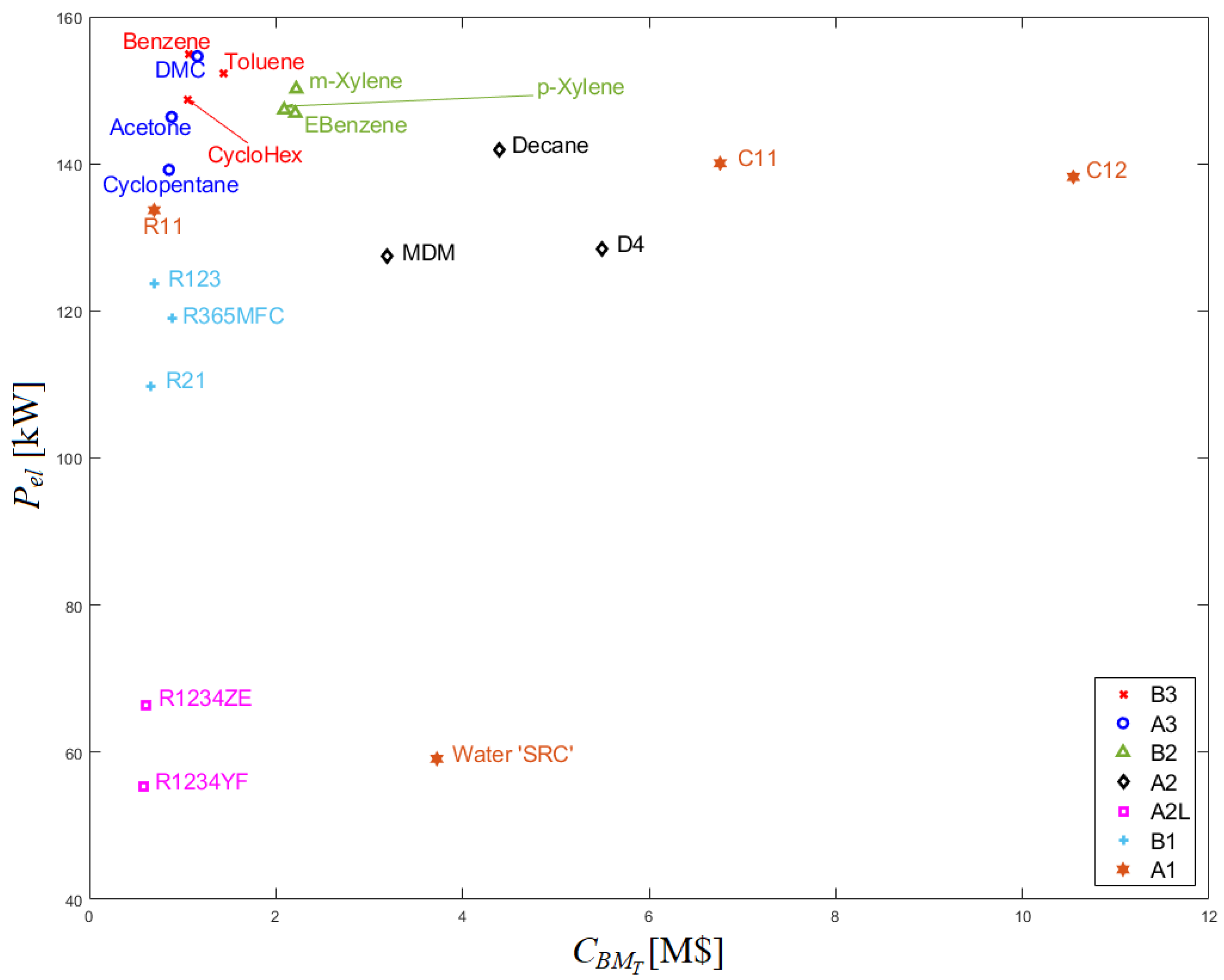
However, the adoption of M-xylene and O-xylene is also not applicable due to the really low condensation pressure, as highlighted by Figure 8. Additionally, these ORC units are characterized by costs ranging from 1.5 to 2.2 M$; thus, approximately 9 k$ per kWel, an unsustainable investment for a bio-gas owner considering that the investment for a bio-gas system is, excluding the ORC, approximately 4.5–5 M$.
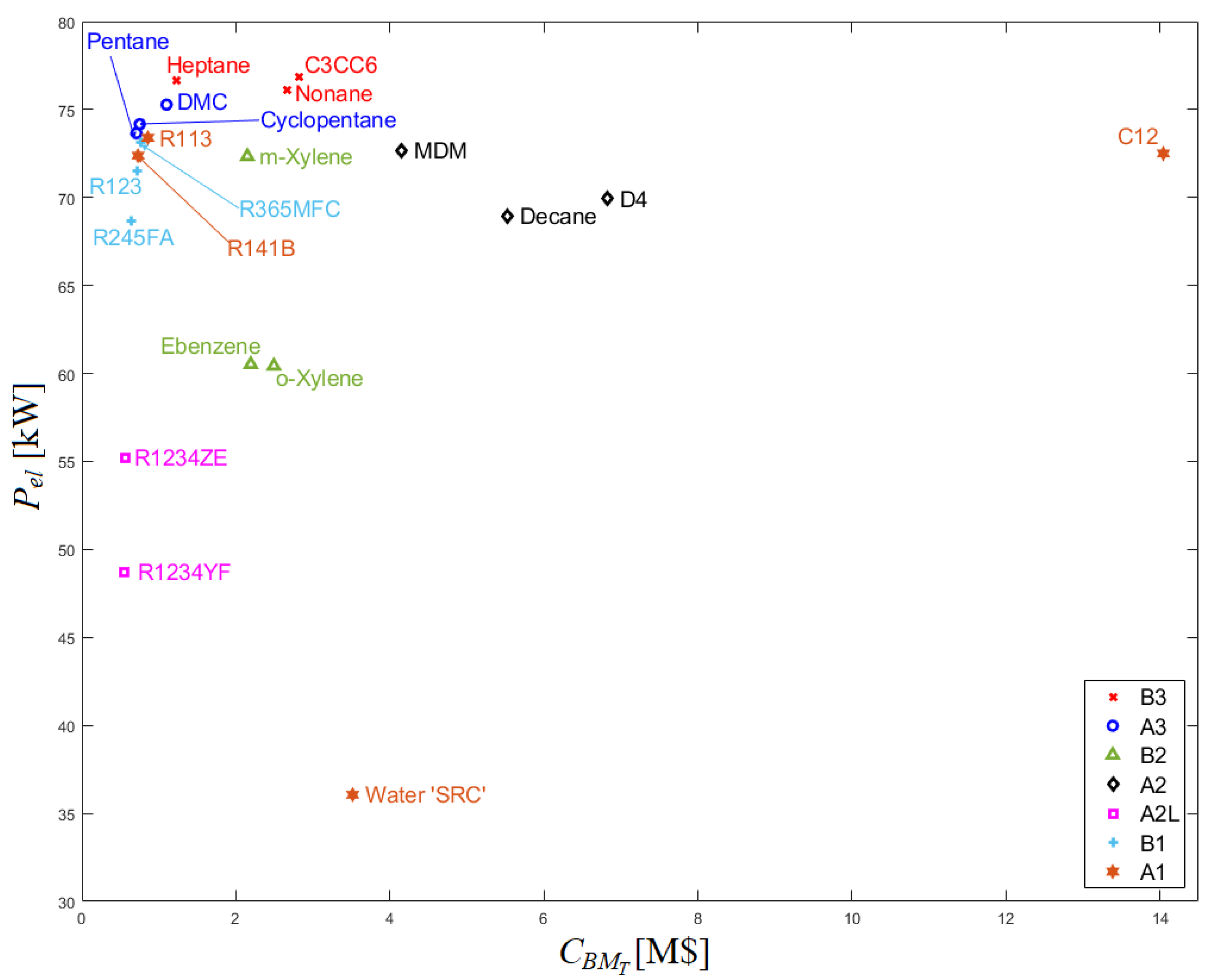
Comparing Figure 5 with Figure 6, it is clear that the adoption of a water loop halved the power producible by the ORC. Therefore, the insertion of a water loop must be avoided. Contrary, the insertion of an oil loop (see Figure 7) adopting Therminol VP-1 guarantees, in the best case (Benzene), a reduction of the ORC net output power of 10% compared to the case without thermal loop (detailed values are given in Table A8 and Table A9). Benzene guarantees a net power output only 5% higher (161.60 kW) if directly coupled with ICE’s exhaust compared to using an oil loop, while the use of DMC, Toluene, Cyclohexane, and M-xylene ensures higher net power output: 6%, 12%, 2%, and 14%. Conversely, the adoption of a water thermal loop provokes a 50% reduction of the power producible by Benzene compared to the cycle adopting Therminol VP-1. Thus, for this application, the use of a thermal oil loop seems the preferable choice. For the sake of clarity, in Table 8, the best and the worst 5 fluids are listed, along with cycle and turbine characteristics.
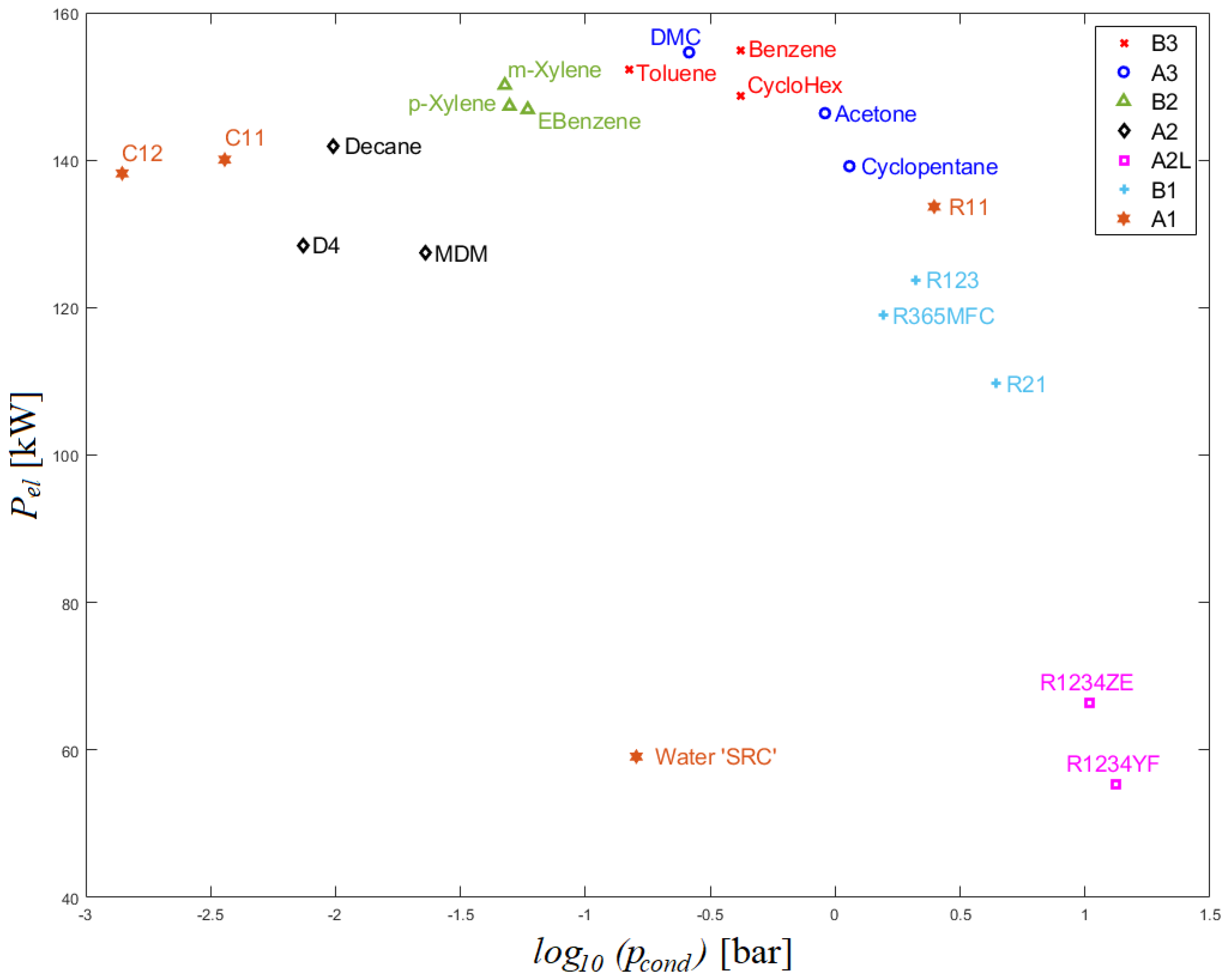
In fact, the results reveal that the cycle can achieve the maximum net power output using Benzene as working fluid, followed by Dimethylcarbonate (DMC), a medium that guarantees a reduction of 0.1% in terms of net output power. Conversely, Toluene, M-xylene, and Cyclohexane guarantee a net output power only 2%, 3%, and 4% lower than the one given with Benzene (see Figure 7).
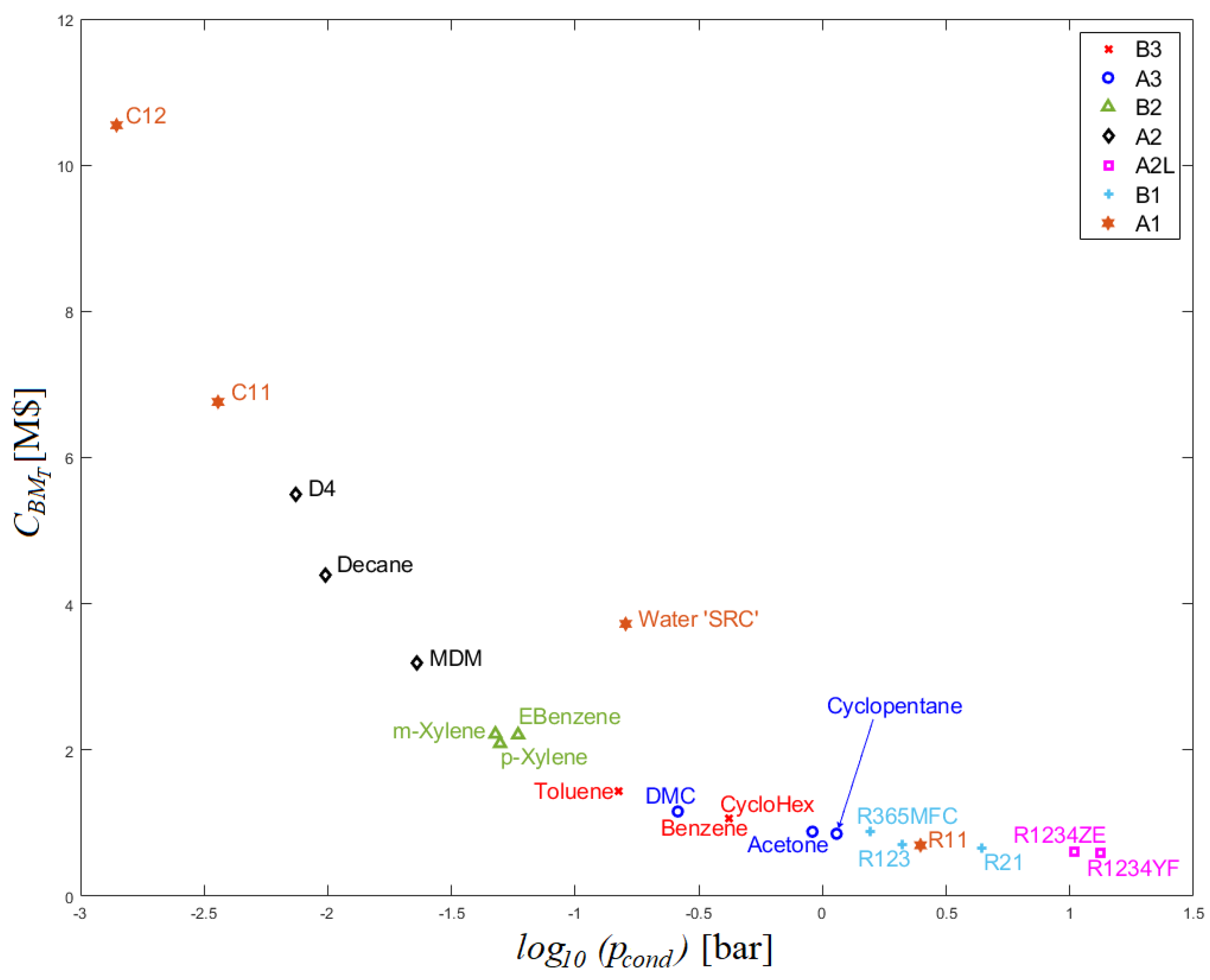
M-xylene and Toluene are not preferable from a technical point of view, and they can be excluded from the list since their condensation pressures are very low compared to other fluids which show reasonable values (see Figure 9 and Table 8). In fact, as depicted in Figure 10, such low condensation pressure leads to higher purchase cost of the ORC unit, besides to more complexity in the plant. In return, the optimization results exhibit that the use of these promising fluids requires a thermal loop as a means to avoid a direct contact between the heat source and the working medium since all of them are flammable. Then, the recuperative configuration linked with a thermal loop and using Benzene as working fluid can be considered the most promising option, despite the fact that its cycle efficiency (20.45%) is lower than the one reachable with Cyclohexane (21.91%) or Toluene (21.68%). Regardless of the fluid, the expander is a 3-stage radial turbine which exhibits an isentropic efficiency higher than 85.2%. Specifically, the higher value is registered with M-xylene (86.4%), while the lower with DMC (85.2%); the turbine using Benzene reaches an isentropic efficiency of 85.5%.
To sum up, the thermodynamic optimization of both SRC and ORC technologies reveals that the use of ORC is more favorable for this application since it guarantees a net power output that can reach 160% of the one generated by SRC. Thus, the authors suggest to adopt the ORC technology for ICE waste heat recovery using an oil thermal loop to guarantee the system safety.
The analysis of the turbine’s parameters (see Table A12) reveals that, among the most promising fluids, Cyclohexane and Benzene show the smaller value of the volumetric flow rate, resulting in a small last stage size parameter (0.0691 m and 0.0690 m, respectively) and, then, leading to a cheaper price of the expander. The latter results in cheaper total price of the ORC unit. These plants are followed by DMC and Toluene, and, finally, the M-xylene. The value of the volumetric flow of M-xylene is too large compared with the one of the other fluids, which results in a large last stage size parameter (0.1825 m), a condition that leads to a higher purchase cost of ORC unit. These results coincide with the ones reported by Astolfi et al. [41], as they mentioned that the use of high critical temperature fluids is associated with very low condensation pressure, which results in a high specific volume at turbine exhaust and, consequently, leads to high costs of the expander, a fact encountered in the case of M-xylene and Toluene.
Therefore, the economic analysis and the determination of the investment costs of the expander reveal that the cycle using Benzene or Cyclohexane as working fluids guarantees the best economic results, as they show the cheapest price for the expander device, which leads to the lowest purchase cost of the ORC unit. Contrary, Toluene and M-xylene are not preferable from an economic point of view since they are characterized by large volumetric flow and large last stage size parameter. So, overall, the higher the turbine cost is, the higher the ORC unit investment cost turns out.
However, it is also interesting to point out that the ORC purchasing costs drop from 8.86 k$ per kWel (no thermal loop and Toluene as working fluid) to 6.8 k$ per kWel (oil thermal loop and Benzene), a more reasonable price for this kind of unit. Therefore, as put forward by the thermodynamic analysis, the costs analysis confirms that Benzene is a good choice for this application.
Since this study examined all the fluids listed in Table A1 and classified them according to their categories, there is a need to note that numerous of them may be nominated as promising fluids for this application, but they are in fact ineligible to be suitable, since many of them have been banned from the application according to many international regulations or because of their environmental impacts. As an example, R123 and R11 in categories B1 and A1, respectively, are candidates to be suitable for use from a thermodynamic point of view in their categories, but they are not adoptable since they are banned from the application by international regulations. Therefore, additional checks and an environmental analysis are required to ensure that the chosen fluids are not banned and are not the source of environment impact.
Thus, the TEWI method was employed to carry out the environmental analysis, and as a means to determine the most environmentally friendly fluids among the promising ones (see Table 9).
Among the 5 best fluids listed in Table 8, the highest value of TEWI is associated with Toluene and DMC, with their GWP values being the highest ones. Benzene ranks third, while the TEWI value of Cyclohexane and M-xylene cannot be estimated due to the lack of numerical values for their GWP. In particular, for Cyclohexane, Li et al. [88] claim that the GWP value of this fluid is “very low”. In addition, given the indirect TEWI linked to the CO2 emissions caused by the generation of the consumed electricity, in the analyzed case, it is not computable. Therefore, with the direct TEWI linked to the GWP, the TEWI value is directly linked to the GWP of the fluid.
The comparison of TEWI values is limited to 3 fluids, and the results show that Benzene is the most environmentally friendly, given its total lifetime CO2 emissions equal to 0.407 ton. Therefore, based on the thermodynamic, economic, and environmental results, to recover the bio-gas ICE waste heat, the best option is to use an ORC unit equipped with a thermal oil loop and using Benzene as working fluid. Thus, considering the Algerian and Italian situation in bio-gas sector, the recuperative ORC configuration using Benzene can improve the electricity production up to 15%, a not-negligible electricity improvement that abate the ICE’s emissions, as well as the thermal pollution.
6. Conclusions
Steam and organic Rankine cycles are viable solutions for waste heat recovery from both fossil and renewable-based plants, as well as industrial processes. However, there is a need for reliable and time-efficient optimization tools that take into account technical, economic, environmental, and safety aspects.
To this end, the authors of the present work developed a versatile tool named Improved Rankine Cycle Plant Designer (IRC-PD), characterized by a wide variety of options that made it adaptable for different cases and give the ability to design and optimize both SRC and ORC units. In addition, as a way to examine it, a real case study of a bio-gas engine was used as the test case. The engine’s nameplate power is 1 MWel, while the design of the waste heat recovery unit is based on real measurements in terms of composition, temperature, and mass flow rate of the engine’s exhaust gases.
Results exhibit that the ORC technology is more appropriate for the examined case compared to SRC technology, mainly because it ensures higher net power output and better economic results. The analysis of the various fluids (more than 120 fluids) for the ORC unit show that Benzene is the most promising fluid from a thermodynamic, as well as an economic, point of view. In particular, the latter ensures the best option for this case by employing it in a recuperative organic Rankine cycle unit which does not recover directly the waste heat source but using an oil loop, where Therminol VP-1 is adopted as thermal medium. The ORC unit, equipped with a 3-stage radial turbine, characterized by an isentropic efficiency of 85.5%, is able to generate 154.92 kWel, a solution that can boost the electricity production of the plant up to 15%.
On the other hand, environmental analysis cannot be considered a major criterion for the selection of the most suitable fluid for this application, since the GWP values of all the promising fluids are very low or approximately zero, as well as the calculated values of TEWI, which are directly related to the fluid GWP.
Therefore, the IRC PD tool is an excellent choice for assessing waste heat recovery for different applications, given the multiple options available on it, the small number of required input from the user, and the ability to evaluate and study the possibility of heat recovery regardless of the field of application. These features make the tool able to design waste heat recovery units based on the ORC and SRC technology with nameplate power ranging from kW to MW.
Author Contributions
Conceptualization, Y.R., K.K.-D., A.S. and A.B.; Data curation, Y.R., K.K.-D., A.S. and A.B.; Methodology, Y.R., K.K.-D., A.S. and A.B.; Validation, Y.R., K.K.-D., A.S. and A.B.; Writing—original draft, A.B.; Writing—review & editing, Y.R., K.K.-D., A.S. and A.B. All authors have read and agreed to the published version of the manuscript.
Funding
This research received no external funding.
Data Availability Statement
Not applicable.
Conflicts of Interest
The authors declare no conflict of interest.
Abbreviations
| CO2 | carbon dioxide |
| GHG | greenhouse gases |
| IEA | International Energy Agency |
| WHRU | plants and waste heat recovery unit |
| RES | renewable energy source |
| EU | European Union |
| PV | PhotoVoltaic |
| IRC-PD | Improved Rankine Cycle Plant Designer |
| SRC | Steam Rankine Cycle |
| ORC | Organic Rankine Cycle |
| ICE | Internal Combustion Engine |
| GA | Genetic Algorithm |
| CEPCI | Chemical engineering plant cost index |
| GWP | Global Warming Potential |
| ODP | Ozone Depletion Potential |
| TEWI | Total equivalent warming impact |
| HC | HydroCarbons |
| HFC | HydroFluoroCarbons |
| HCFC | HydroChloroFluoroCarbons |
| CFC | ChloroFluoroCarbons |
| PFC | PerFluoroCarbons |
| HFO | HydroFluoroOlefins |
| MHE | Main Heat Exchanger |
| TL | Thermal Loop |
| HX | Heat Exchange |
| A | Axial |
| R | Radial |
| Symbols | |
| T | temperature ( or °C) |
| standard boiling point temperature ( or °C) | |
| critical temperature ( or °C) | |
| turning point temperature ( or °C) | |
| P | power (W) |
| p | pressure (bar) |
| h | specific enthalpy (kJ kg−1) |
| E | recuperator efficiency (-) |
| s | specific entropy (J kg−1 K−1) |
| bare module cost ($) | |
| purchased equipment cost base conditions ($) | |
| A | heat transfer surface (m2) |
| cost of the site ($) | |
| operation and maintenance cost ($) | |
| i | interest rate (%) |
| f | plant availability factor (-) |
| corporate tax rate (%) | |
| capital recovery factor ($) | |
| load coefficient (-) | |
| M | Refrigerant charge (kg) |
| mass flow rate (kg s−1) | |
| n | system operating lifetime (year) |
| Net Present Value ($) | |
| Size Parameter (m) | |
| Cash Flow ($) | |
| Profitability Index (-) | |
| Simple PayBack (year) | |
| Levelized Cost Of Energy ($ kW−1) | |
| L | annual leakage (kg year−1) |
| electricity sell price ($) | |
| annual electricity production (kWh) | |
| annual operating hour (hour) | |
| annual incomes ($) | |
| Total equivalent warming impact (ton CO2,eq) | |
| mean peripheral speed (m s−1) | |
| volumetric flow rate (m3 s−1) | |
| Subscripts | |
| electrical | |
| Exp | expander |
| inlet | |
| hot source | |
| isentropic | |
| mechanical | |
| maximum | |
| minimum | |
| outlet | |
| evaporation | |
| P | Pump |
| Pinch Point | |
| ST | steam turbine |
| saturated vapor | |
| turning point | |
| T | turbine |
| thermal oil | |
| t | total |
| working fluid | |
| Greek symbols | |
| recycling factor (-) | |
| carbon dioxide emission factor (kgCO2,eq kWh−1) | |
| difference | |
| efficiency (%) | |
| Slope (-) |
Appendix A. Thermodynamic Points Computations
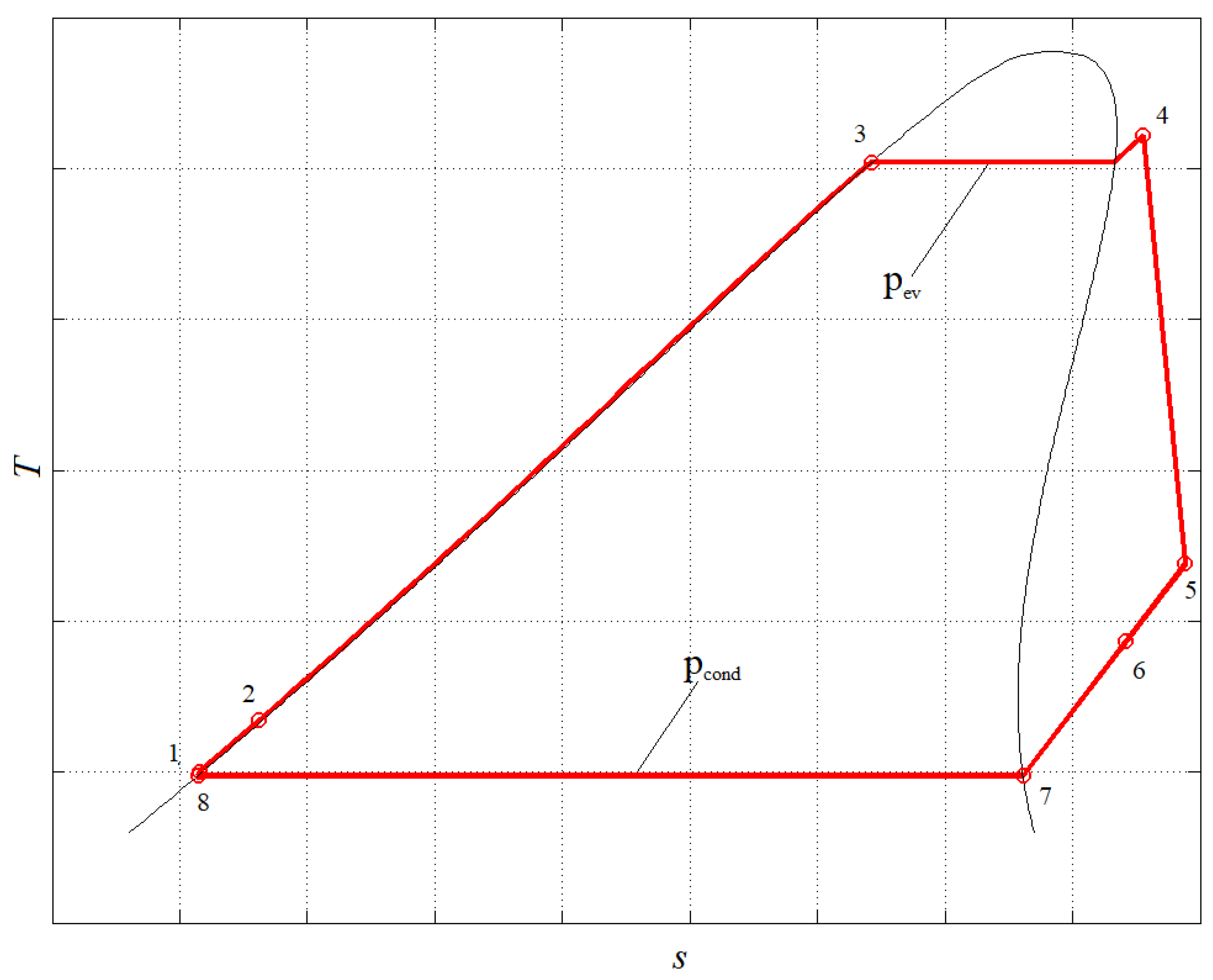
The equations implemented into the IRC-PD tool for the recuperative configuration are listed in the following considering the thermodynamic points shown in Figure A1.
Figure A1.
T-s diagram of the recuperative cycle implemented in the code. The thermodynamic state points are included in the graph to better identify their position.
Figure A1.
T-s diagram of the recuperative cycle implemented in the code. The thermodynamic state points are included in the graph to better identify their position.

The net output power is computed according to the selected configuration.
For the configuration without thermal loop, it is computed as:
while, for the configuration including a thermal loop, it is given as:
For the configuration including a thermal loop and air-cooled condenser, the net output power is computed as:
while, for the configuration with an air-cooled condenser and without a thermal loop, it is derived from:
The list of the available working fluids is presented in Table A1.

Table A1.
HCs, HFCs, Siloxanes, PCFs, HCFCs, CFCs, and other candidates implemented in the code.
| HCs | HFCs | Siloxanes | PCFs | HCFCs | CFCs | Cryogens | |
|---|---|---|---|---|---|---|---|
| N-octane | N-decane | R32 | D4 | C4F10 | R123 | R11 | Neon |
| 1-butene | Neopentane | R125 | D5 | C5F12 | R124 | R113 | Nitrogen |
| Acetone | N-heptane | R134A | D6 | R116 | R141B | R114 | Ohydrogen |
| Benzene | N-hexane | R13I1 | MD2M | R1216 | R142B | R115 | Oxygen |
| C1CC6 | N-nonane | R143A | MD3M | R14 | R21 | R12 | Phydrogen |
| C2BUTENE | N-Undecane | R152A | MD4M | R161 | R22 | R13 | Xenon |
| C3CC6 | O-xylene | R227EA | MDM | R218 | Argon | ||
| Cyclohexane | Pentane | R23 | MM | CO | |||
| Cyclopentane | Propane | R236EA | Deuterium | ||||
| Cyclopropane | Propene | R236FA | Fluorine | ||||
| E-Benzene | Propyne | RC318 | Helium | ||||
| Ethylene | P-xylene | R245CA | Hydrogen | ||||
| Isobutane | R365MFC | R245FA | Krypton | ||||
| Isobutene | SES36 | R40 | |||||
| N-dodecane | Toluene | R404A | |||||
| Isohexane | trans-Butene | R407C | |||||
| Isopentane | Iso-octane | R41 | |||||
| M-xylene | R410A | ||||||
| N-butane | R507A | ||||||
| HFOs | Ethers | FAMEs | Inorganics | Alcohols & Esters | Others | ICF | |
| R1233zd(E) | DEE | Mlinolea | Ammonia | Ethanol | d2o | ThermVP1 | |
| R1234YF | DME | Mlinolen | CO2 | Methanol | Novec649 | DowQ | |
| R1234ZDE | RE143A | Moleate | Water | DMC | Propylene | Therm66 | |
| R1234ZE | RE245cb2 | Mpalmita | H2S | ||||
| R1234ze(Z) | RE245fa2 | Mstearat | HCL | ||||
| RE347MCC | SO2 |
Figure A2.
Steps involved during the optimization using the IRC-PD Tool.

Appendix B. Parameters Adopted in the Economic Analysis
In order to perform the economic analysis, the logarithmic mean temperature approach is used to compute the heat exchanger area and the adopted formula is given in Equation (A21) [90]. The exchange heat is given multiplying the overall heat transfer coefficient U, by the area of exchange A, and the logarithmic mean temperature Tlm.
Thus, for the computation of the area of exchange for each heat exchanger, the overall heat transfer coefficient, U, is selected according to Dimian and Bildea [91] and given as follows:
The coefficients used for preforming the economic analysis of each device are listed in Table A2 and Table A3.
Table A2.
Parameters and range of applications used in the equations.
| Component | N | Size Range | K1 K2 K3 | C1 C2 C3 | B1 B2 | FM | FBM | Ref. |
|---|---|---|---|---|---|---|---|---|
| Shell and tube heat exchanger | A [m2] | 10–1000 | 4.3247 | 0.03881 | 1.63 1.66 | 1 | - | [46] |
| −0.3030 | −0.11272 | |||||||
| 0.1634 | 0.08183 | |||||||
| Pump | P [kW] | 1–300 | 3.3892 | −0.3935 | 1.89 1.35 | 1.575 | - | [46] |
| 0.0536 | 0.3957 | |||||||
| 0.1538 | −0.00226 | |||||||
| Pump electrical motor | P [kW] | - | 2.4604 | - | - | - | 1.5 | [46] |
| 1.4191 | ||||||||
| −0.1798 |
Appendix C. Optimized Variables for the Different SRC and ORC Configurations
The thermodynamic optimization of SRC in terms of net power output is carried out adopting the basic configuration of SRC and a multi-stage steam turbine in which a specific enthalpy drop of 150 kJ kg−1 and a fixed rotational speed equal to 6000 rpm [92] are adopted. In the case of a steam cycle coupled with a water loop, the optimization process is unfeasible if the lower bound of the evaporation pressure is set equal to 15 bar. So, to show the code ability of providing a solution (unfeasible from the technical point of view), the lower bound of the evaporation pressure is set equal to 1 bar.
Table A4.
Results of the thermodynamic optimization and economic analysis of the SRC without thermal loop.
Table A4.
Results of the thermodynamic optimization and economic analysis of the SRC without thermal loop.
| TIT | Stages | ||||||||||
|---|---|---|---|---|---|---|---|---|---|---|---|
| [kW] | [°C] | [°C] | [bar] | [bar] | [%] | [%] | [-] | [°C] | [-] | ||
| 96.38 | 156.9 | 477.9 | 19.22 | 0.15 | 13.96 | 0.528 | 25.0 | 10.1 | 7 | 3.8302 | 3.502 |
Table A5.
Results of the thermodynamic optimization and economic analysis of the SRC adopting a water thermal loop.
Table A5.
Results of the thermodynamic optimization and economic analysis of the SRC adopting a water thermal loop.
| TIT | Stages | |||||||||||
|---|---|---|---|---|---|---|---|---|---|---|---|---|
| [kW] | [°C] | [°C] | [°C] | [bar] | [bar] | [%] | [%] | [-] | [°C] | [-] | ||
| 36.06 | 150.9 | 140 | 134.9 | 1.82 | 0.16 | 4.92 | 0.397 | 25.1 | 10.8 | 3 | 3.517 | 3.225 |
Table A6.
Results of the thermodynamic optimization and economic analysis of the SRC adopting an oil thermal loop.
Table A6.
Results of the thermodynamic optimization and economic analysis of the SRC adopting an oil thermal loop.
| TIT | Stages | |||||||||||
|---|---|---|---|---|---|---|---|---|---|---|---|---|
| [kW] | [°C] | [°C] | [°C] | [bar] | [bar] | [%] | [%] | [-] | [°C] | [-] | ||
| 59.10 | 190.9 | 180.9 | 333.9 | 15.00 | 0.16 | 9.45 | 0.403 | 25.4 | 10.6 | 6 | 3.725 | 3.433 |
Table A7.
Most promising ORC fluids in the case of direct exchange between ICE’s exhaust and the cycle.
Table A7.
Most promising ORC fluids in the case of direct exchange between ICE’s exhaust and the cycle.
| Fluid | E | Stages | |||||||||
|---|---|---|---|---|---|---|---|---|---|---|---|
| [kW] | [°C] | [°C] | [bar] | [bar] | [%] | [%] | [-] | [°C] | [°C] | [-] | |
| Toluene | 169.89 | 133.9 | 329.9 | 33.5 | 0.13 | 51 | 23.13 | 0.847 | 25.6 | 10.3 | 3-R |
| M-xylene | 169.50 | 113.9 | 306.9 | 20.98 | 0.04 | 35 | 21.94 | 0.844 | 26.1 | 10.1 | 3-R |
| O-xylene | 169.27 | 135.9 | 332.9 | 23.02 | 0.03 | 47 | 23.17 | 0.838 | 25.4 | 10.1 | 3-R |
| P-xylene | 169.08 | 129.9 | 330.9 | 25.34 | 0.04 | 44 | 22.78 | 0.839 | 25.2 | 10.1 | 3-R |
| E-Benzene | 167.37 | 147.9 | 317.9 | 23.85 | 0.05 | 62 | 23.65 | 0.843 | 25.3 | 10.5 | 3-R |
Table A8.
Most promising fluids in the case of adopting an ORC and a water loop.
| Fluid | E | Stages | ||||||||||
|---|---|---|---|---|---|---|---|---|---|---|---|---|
| [kW] | [°C] | [°C] | [°C] | [bar] | [bar] | [%] | [%] | [-] | [°C] | [°C] | [-] | |
| C3CC6 | 76.84 | 150.9 | 140 | 131.9 | 0.34 | 0.03 | 49 | 11.00 | 0.903 | 26.7 | 10.2 | 2-A |
| Heptane | 76.64 | 150.9 | 140 | 133.9 | 1.84 | 0.21 | 53 | 10.97 | 0.891 | 25.5 | 10.2 | 2-A |
| Nonane | 76.13 | 151.9 | 140 | 124.9 | 0.41 | 0.03 | 45 | 10.90 | 0.902 | 26.4 | 10.2 | 2-A |
| Octane | 75.53 | 151.9 | 140 | 128.9 | 0.82 | 0.08 | 50 | 10.81 | 0.901 | 27.4 | 10.2 | 2-A |
| DMC | 75.28 | 150.9 | 140 | 131.9 | 2.35 | 0.27 | 17 | 10.77 | 0.887 | 26.2 | 10.4 | 2-A |
Table A9.
Most promising fluids in the case of adopting an ORC and an oil loop.
| Fluid | E | Stages | ||||||||||
|---|---|---|---|---|---|---|---|---|---|---|---|---|
| [kW] | [°C] | [°C] | [°C] | [bar] | [bar] | [%] | [%] | [-] | [°C] | [°C] | [-] | |
| Benzene | 154.92 | 121.9 | 111.9 | 258.9 | 32.25 | 0.42 | 53 | 20.45 | 0.855 | 26.4 | 10.8 | 3-R |
| DMC | 154.62 | 122.9 | 112.9 | 266.9 | 34.94 | 0.26 | 44 | 20.46 | 0.852 | 25.4 | 10.6 | 3-R |
| Toluene | 152.21 | 150.9 | 140.9 | 250.9 | 15.68 | 0.15 | 77 | 21.68 | 0.864 | 25.8 | 11.4 | 3-R |
| M-xylene | 150.17 | 149.9 | 139.9 | 241.9 | 7.58 | 0.05 | 68 | 21.33 | 0.868 | 25.3 | 10.2 | 3-R |
| Cyclohex | 148.75 | 162.9 | 152.9 | 275.9 | 34.03 | 0.42 | 78 | 21.91 | 0.852 | 26.0 | 11.2 | 3-R |
Table A10.
Economic analysis results of the ORC fluids in the case of a direct exchange between the ICE exhaust and the working fluid.
Table A10.
Economic analysis results of the ORC fluids in the case of a direct exchange between the ICE exhaust and the working fluid.
| Fluid | |||||
|---|---|---|---|---|---|
| [%] | |||||
| Toluene | 1.505 | 1.023 | 67.98 | 0.1081 | 3.45 |
| E-Benzene | 2.062 | 1.607 | 77.94 | 0.1630 | 7.66 |
| P-xylene | 2.197 | 1.716 | 78.10 | 0.1729 | 8.88 |
| M-xylene | 2.257 | 1.774 | 78.60 | 0.1783 | 9.32 |
| O-xylene | 2.383 | 1.904 | 79.87 | 0.1901 | 10.95 |
Table A11.
Economic analysis results of the ORC fluids in the case of using water as heat transfer medium in the thermal loop.
Table A11.
Economic analysis results of the ORC fluids in the case of using water as heat transfer medium in the thermal loop.
| Fluid | |||||
|---|---|---|---|---|---|
| [%] | |||||
| DMC | 1.100 | 0.707 | 64.31 | 0.0929 | 1.68 |
| Heptane | 1.225 | 0.853 | 69.61 | 0.1101 | 2.25 |
| Octane | 1.791 | 1.406 | 78.49 | 0.1735 | 5.49 |
| Nonane | 2.670 | 2.279 | 85.35 | 0.2692 | 13.24 |
| C3CC6 | 2.825 | 2.444 | 86.50 | 0.2869 | 15.00 |
Table A12.
Economic analysis results of the ORC fluids in the case of using oil as heat transfer medium in the thermal loop.
Table A12.
Economic analysis results of the ORC fluids in the case of using oil as heat transfer medium in the thermal loop.
| Fluid | |||||
|---|---|---|---|---|---|
| [%] | |||||
| Benzene | 1.067 | 0.625 | 58.54 | 0.0690 | 1.23 |
| DMC | 1.159 | 0.752 | 62.86 | 0.0817 | 1.74 |
| Toluene | 1.440 | 1.031 | 71.64 | 0.1089 | 3.00 |
| M-xylene | 2.218 | 1.820 | 82.06 | 0.1825 | 8.31 |
| Cyclohex | 1.058 | 0.625 | 59.07 | 0.0691 | 1.23 |
References
- Horowitz, C.A. Paris agreement. Int. Leg. Mater. 2016, 55, 740–755. [Google Scholar] [CrossRef]
- International Energy Agency. IEA statistics, 2019. In CO2 Emissions from Fuel Combustion: Highlights; International Energy Agency: Paris, France, 2019. [Google Scholar]
- Meinshausen, M.; Meinshausen, N.; Hare, W.; Raper, S.C.; Frieler, K.; Knutti, R.; Frame, D.J.; Allen, M.R. Greenhouse-gas emission targets for limiting global warming to 2 C. Nature 2009, 458, 1158–1162. [Google Scholar] [CrossRef] [PubMed]
- Sikora, A. European Green Deal–legal and financial challenges of the climate change. In ERA Forum; Springer: Berlin/Heidelberg, Germany, 2021; Volume 21, pp. 681–697. [Google Scholar]
- Skjærseth, J.B. Towards a European Green Deal: The evolution of EU climate and energy policy mixes. Int. Environ. Agreem. Politics Law Econ. 2021, 21, 25–41. [Google Scholar] [CrossRef]
- Algerian Ministry of Energy. Energies Nouvelles, Renouvelables et Maitrise de l’Energie; Algiers, Algeria. 2021. Available online: https://www.energy.gov.dz/?rubrique=energies-nouvellesrenouvelables-et-maitrise-de-lrenergie (accessed on 4 September 2021).
- Bouzid, Z.; Ghellai, N. Overview of solar potential, state of the art and future of photovoltaic installations in Algeria. Int. J. Renew. Energy Res. IJRER 2015, 5, 427–434. [Google Scholar]
- Bouraiou, A.; Necaibia, A.; Boutasseta, N.; Mekhilef, S.; Dabou, R.; Ziane, A.; Sahouane, N.; Attoui, I.; Mostefaoui, M.; Touaba, O. Status of renewable energy potential and utilization in Algeria. J. Clean. Prod. 2020, 246, 119011. [Google Scholar] [CrossRef]
- Akbi, A.; Saber, M.; Aziza, M.; Yassaa, N. An overview of sustainable bioenergy potential in Algeria. Renew. Sustain. Energy Rev. 2017, 72, 240–245. [Google Scholar] [CrossRef]
- Campana, F.; Bianchi, M.; Branchini, L.; De Pascale, A.; Peretto, A.; Baresi, M.; Fermi, A.; Rossetti, N.; Vescovo, R. ORC waste heat recovery in European energy intensive industries: Energy and GHG savings. Energy Convers. Manag. 2013, 76, 244–252. [Google Scholar] [CrossRef]
- Benato, A. Improving the efficiency of a cataphoresis oven with a cogenerative organic Rankine cycle unit. Therm. Sci. Eng. Prog. 2018, 5, 182–194. [Google Scholar] [CrossRef]
- Papapetrou, M.; Kosmadakis, G.; Cipollina, A.; La Commare, U.; Micale, G. Industrial waste heat: Estimation of the technically available resource in the EU per industrial sector, temperature level and country. Appl. Therm. Eng. 2018, 138, 207–216. [Google Scholar] [CrossRef]
- Cavazzini, G.; Bari, S.; McGrail, P.; Benedetti, V.; Pavesi, G.; Ardizzon, G. Contribution of Metal-Organic-Heat Carrier nanoparticles in a R245fa low-grade heat recovery Organic Rankine Cycle. Energy Convers. Manag. 2019, 199, 111960. [Google Scholar] [CrossRef]
- Fierro, J.J.; Escudero-Atehortua, A.; Nieto-Londoño, C.; Giraldo, M.; Jouhara, H.; Wrobel, L.C. Evaluation of waste heat recovery technologies for the cement industry. Int. J. Thermofluids 2020, 7, 100040. [Google Scholar] [CrossRef]
- Prando, D.; Renzi, M.; Gasparella, A.; Baratieri, M. Monitoring of the energy performance of a district heating CHP plant based on biomass boiler and ORC generator. Appl. Therm. Eng. 2015, 79, 98–107. [Google Scholar] [CrossRef]
- Pezzuolo, A.; Benato, A.; Stoppato, A.; Mirandola, A. Fluid selection and plant configuration of an ORC-biomass fed system generating heat and/or power. Energy Procedia 2016, 101, 822–829. [Google Scholar] [CrossRef]
- Benato, A.; Macor, A. Biogas engine waste heat recovery using organic Rankine cycle. Energies 2017, 10, 327. [Google Scholar] [CrossRef]
- DeLovato, N.; Sundarnath, K.; Cvijovic, L.; Kota, K.; Kuravi, S. A review of heat recovery applications for solar and geothermal power plants. Renew. Sustain. Energy Rev. 2019, 114, 109329. [Google Scholar] [CrossRef]
- Freeman, J.; Hellgardt, K.; Markides, C.N. Working fluid selection and electrical performance optimisation of a domestic solar-ORC combined heat and power system for year-round operation in the UK. Appl. Energy 2017, 186, 291–303. [Google Scholar] [CrossRef] [Green Version]
- The Mathworks. Guide, MATLAB User’s; The Mathworks: Natick, MA, USA, 2021. [Google Scholar]
- Pezzuolo, A.; Benato, A.; Stoppato, A.; Mirandola, A. The ORC-PD: A versatile tool for fluid selection and Organic Rankine Cycle unit design. Energy 2016, 102, 605–620. [Google Scholar] [CrossRef]
- The Mathworks. Global Optimization Toolbox. 2021. Available online: https://it.mathworks.com/help/gads/?s_tid=srchbrcm (accessed on 4 September 2021).
- NIST. NIST Reference Fluid Thermodynamic and Transport Properties Database (REFPROP): Version 9.1. 2010. Available online: http://www.nist.gov/srd/nist23.cfm (accessed on 4 September 2021).
- Bell, I.H.; Wronski, J.; Quoilin, S.; Lemort, V. Pure and Pseudo-pure Fluid Thermophysical Property Evaluation and the Open-Source Thermophysical Property Library CoolProp. Ind. Eng. Chem. Res. 2014, 53, 2498–2508. [Google Scholar] [CrossRef] [Green Version]
- ASHRAE. ANSI/ASHRAE 34-2019. Designation and Safety Classification of Refrigerants. 2021. Available online: https://www.ashrae.org/technical-resources/standards-and-guidelines/ashrae-refrigerant-designations (accessed on 4 September 2021).
- Nord, L.O.; Martelli, E.; Bolland, O. Weight and power optimization of steam bottoming cycle for offshore oil and gas installations. Energy 2014, 76, 891–898. [Google Scholar] [CrossRef] [Green Version]
- Pierobon, L.; Benato, A.; Scolari, E.; Haglind, F.; Stoppato, A. Waste heat recovery technologies for offshore platforms. Appl. Energy 2014, 136, 228–241. [Google Scholar] [CrossRef] [Green Version]
- Branchini, L.; De Pascale, A.; Peretto, A. Systematic comparison of ORC configurations by means of comprehensive performance indexes. Appl. Therm. Eng. 2013, 61, 129–140. [Google Scholar] [CrossRef]
- Shokati, N.; Ranjbar, F.; Yari, M. Exergoeconomic analysis and optimization of basic, dual-pressure and dual-fluid ORCs and Kalina geothermal power plants: A comparative study. Renew. Energy 2015, 83, 527–542. [Google Scholar] [CrossRef]
- Meinel, D.; Wieland, C.; Spliethoff, H. Effect and comparison of different working fluids on a two-stage organic rankine cycle (ORC) concept. Appl. Therm. Eng. 2014, 63, 246–253. [Google Scholar] [CrossRef]
- Weith, T.; Heberle, F.; Preißinger, M.; Brüggemann, D. Performance of siloxane mixtures in a high-temperature Organic Rankine Cycle considering the heat transfer characteristics during evaporation. Energies 2014, 7, 5548–5565. [Google Scholar] [CrossRef]
- Oyewunmi, O.A.; Taleb, A.I.; Haslam, A.J.; Markides, C.N. An assessment of working-fluid mixtures using SAFT-VR Mie for use in organic Rankine cycle systems for waste-heat recovery. Comput. Therm. Sci. Int. J. 2014, 6, 266. [Google Scholar] [CrossRef]
- Heberle, F.; Brüggemann, D. Thermo-economic analysis of zeotropic mixtures and pure working fluids in organic Rankine cycles for waste heat recovery. Energies 2016, 9, 226. [Google Scholar] [CrossRef]
- Venkatarathnam, G.; Timmerhaus, K.D. Cryogenic Mixed Refrigerant Processes; Springer: Berlin/Heidelberg, Germany, 2008. [Google Scholar]
- Chys, M.; van den Broek, M.; Vanslambrouck, B.; De Paepe, M. Potential of zeotropic mixtures as working fluids in organic Rankine cycles. Energy 2012, 44, 623–632. [Google Scholar] [CrossRef]
- Bell, K.; Ghaly, M. An Approximate Generalized Design Method for Multicomponent-Partial Condenser. AIChEn Symp. Ser. 1972, 69, 72–79. [Google Scholar]
- Shah, M.M. Chart correlation for saturated boiling heat transfer: Equations and further study. ASHRAE Trans. 1982, 88, 185–196. [Google Scholar]
- Bahadori, A.; Vuthaluru, H.B. Estimation of performance of steam turbines using a simple predictive tool. Appl. Therm. Eng. 2010, 30, 1832–1838. [Google Scholar] [CrossRef]
- Macchi, E.; Perdichizzi, A. Efficiency prediction for axial-flow turbines operating with nonconventional fluids. J. Eng. Gas Turbines Power 1981, 103, 718–724. [Google Scholar] [CrossRef]
- Perdichizzi, A.; Lozza, G. Design criteria and efficiency prediction for radial inflow turbines. In Proceedings of the ASME 1987 International Gas Turbine Conference and Exhibition, Anaheim, CA, USA, 31 May–4 June 1987; American Society of Mechanical Engineers: New York, NY, USA, 1987. [Google Scholar]
- Astolfi, M.; Romano, M.C.; Bombarda, P.; Macchi, E. Binary ORC (Organic Rankine Cycles) power plants for the exploitation of medium-low temperature geothermal sources—Part B: Techno-economic optimization. Energy 2014, 66, 435–446. [Google Scholar] [CrossRef]
- Martelli, E.; Capra, F.; Consonni, S. Numerical optimization of combined heat and power organic Rankine cycles—Part A: Design optimization. Energy 2015, 90, 310–328. [Google Scholar] [CrossRef]
- Macchi, E.; Astolfi, M. Organic Rankine Cycle (ORC) Power Systems: Technologies and Applications; Woodhead Publishing: Shaxton, UK, 2016. [Google Scholar]
- Liu, B.T.; Chien, K.H.; Wang, C.C. Effect of working fluids on organic Rankine cycle for waste heat recovery. Energy 2004, 29, 1207–1217. [Google Scholar] [CrossRef]
- Wang, X.; Levy, E.K.; Pan, C.; Romero, C.E.; Banerjee, A.; Rubio-Maya, C.; Pan, L. Working fluid selection for organic Rankine cycle power generation using hot produced supercritical CO2 from a geothermal reservoir. Appl. Therm. Eng. 2019, 149, 1287–1304. [Google Scholar] [CrossRef]
- Turton, R.; Bailie, R.C.; Whiting, W.B.; Shaeiwitz, J.A. Analysis, Synthesis and Design of Chemical Processes; Pearson Education: London, UK, 2018. [Google Scholar]
- Smith, R. Chemical Process: Design and Integration; John Wiley & Sons: Hoboken, NJ, USA, 2016. [Google Scholar]
- Toffolo, A.; Lazzaretto, A.; Manente, G.; Paci, M. A multi-criteria approach for the optimal selection of working fluid and design parameters in Organic Rankine Cycle systems. Appl. Energy 2014, 121, 219–232. [Google Scholar] [CrossRef]
- Manesh, M.K.; Navid, P.; Marigorta, A.B.; Amidpour, M.; Hamedi, M. New procedure for optimal design and evaluation of cogeneration system based on advanced exergoeconomic and exergoenvironmental analyses. Energy 2013, 59, 314–333. [Google Scholar] [CrossRef]
- Zhang, X.; Cao, M.; Yang, X.; Guo, H.; Wang, J. Economic analysis of organic Rankine cycle using R123 and R245fa as working fluids and a demonstration project report. Appl. Sci. 2019, 9, 288. [Google Scholar] [CrossRef] [Green Version]
- ANSI/ASHRAE. ANSI/ASHRAE Standard 34-2010, Designation and Safety Classification of Refrigerants; ANSI/ASHRAE: Peachtree Corners, GA, USA, 2010. [Google Scholar]
- United Nations Environment Programme. Ozone Secretariat. Handbook for the Montreal Protocol on Substances That Deplete the Ozone Layer; UNEP/Earthprint: Kenya, Nairobi, 2006. [Google Scholar]
- European Union. Directive 2006/40/EC of the European Parliament and of the Council of 17 May 2006 relating to emissions from air-conditioning systems in motor vehicles and Amending Council Directive 70/156/EEC. Off. J. Eur. Union L 2006, 161, 12–18. [Google Scholar]
- Gullo, P.; Tsamos, K.M.; Hafner, A.; Banasiak, K.; Yunting, T.G.; Tassou, S.A. Crossing CO2 equator with the aid of multi-ejector concept: A comprehensive energy and environmental comparative study. Energy 2018, 164, 236–263. [Google Scholar] [CrossRef]
- Ye, Z.; Yang, J.; Shi, J.; Chen, J. Thermo-economic and environmental analysis of various low-GWP refrigerants in Organic Rankine cycle system. Energy 2020, 199, 117344. [Google Scholar] [CrossRef]
- Bellos, E.; Tzivanidis, C. A theoretical comparative study of CO2 cascade refrigeration systems. Appl. Sci. 2019, 9, 790. [Google Scholar] [CrossRef] [Green Version]
- Material Safety Data Sheets. Available online: https://www.nationalref.com/technical/msds/ (accessed on 4 September 2021).
- Collings, P.; Yu, Z.; Wang, E. A dynamic organic Rankine cycle using a zeotropic mixture as the working fluid with composition tuning to match changing ambient conditions. Appl. Energy 2016, 171, 581–591. [Google Scholar] [CrossRef] [Green Version]
- Vaja, I.; Gambarotta, A. Internal combustion engine (ICE) bottoming with organic Rankine cycles (ORCs). Energy 2010, 35, 1084–1093. [Google Scholar] [CrossRef]
- Liu, P.; Shu, G.; Tian, H.; Wang, X. Engine load effects on the energy and exergy performance of a medium cycle/organic Rankine cycle for exhaust waste heat recovery. Entropy 2018, 20, 137. [Google Scholar] [CrossRef] [PubMed] [Green Version]
- GE. GE Power Generation. 2016. Available online: https://powergen.gepower.com/applications/bio-gas.html (accessed on 4 September 2021).
- Bombarda, P.; Invernizzi, C.M.; Pietra, C. Heat recovery from Diesel engines: A thermodynamic comparison between Kalina and ORC cycles. Appl. Therm. Eng. 2010, 30, 212–219. [Google Scholar] [CrossRef] [Green Version]
- Pan, M.; Zhu, Y.; Bian, X.; Liang, Y.; Lu, F.; Ban, Z. Theoretical analysis and comparison on supercritical CO2 based combined cycles for waste heat recovery of engine. Energy Convers. Manag. 2020, 219, 113049. [Google Scholar] [CrossRef]
- Yu, G.; Shu, G.; Tian, H.; Huo, Y.; Zhu, W. Experimental investigations on a cascaded steam-/organic-Rankine-cycle (RC/ORC) system for waste heat recovery (WHR) from diesel engine. Energy Convers. Manag. 2016, 129, 43–51. [Google Scholar] [CrossRef]
- Liu, X.; Nguyen, M.Q.; Chu, J.; Lan, T.; He, M. A novel waste heat recovery system combing steam Rankine cycle and organic Rankine cycle for marine engine. J. Clean. Prod. 2020, 265, 121502. [Google Scholar] [CrossRef]
- Andreasen, J.G.; Meroni, A.; Haglind, F. A comparison of organic and steam Rankine cycle power systems for waste heat recovery on large ships. Energies 2017, 10, 547. [Google Scholar] [CrossRef] [Green Version]
- Yang, F.; Dong, X.; Zhang, H.; Wang, Z.; Yang, K.; Zhang, J.; Wang, E.; Liu, H.; Zhao, G. Performance analysis of waste heat recovery with a dual loop organic Rankine cycle (ORC) system for diesel engine under various operating conditions. Energy Convers. Manag. 2014, 80, 243–255. [Google Scholar] [CrossRef]
- Wang, E.; Zhang, H.; Fan, B.; Ouyang, M.; Yang, F.; Yang, K.; Wang, Z.; Zhang, J.; Yang, F. Parametric analysis of a dual-loop ORC system for waste heat recovery of a diesel engine. Appl. Therm. Eng. 2014, 67, 168–178. [Google Scholar] [CrossRef]
- Song, J.; Gu, C.W. Parametric analysis of a dual loop Organic Rankine Cycle (ORC) system for engine waste heat recovery. Energy Convers. Manag. 2015, 105, 995–1005. [Google Scholar] [CrossRef]
- Shu, G.; Gao, Y.; Tian, H.; Wei, H.; Liang, X. Study of mixtures based on hydrocarbons used in ORC (Organic Rankine Cycle) for engine waste heat recovery. Energy 2014, 74, 428–438. [Google Scholar] [CrossRef]
- Wang, E.; Zhang, H.; Fan, B.; Ouyang, M.; Zhao, Y.; Mu, Q. Study of working fluid selection of organic Rankine cycle (ORC) for engine waste heat recovery. Energy 2011, 36, 3406–3418. [Google Scholar] [CrossRef]
- Tian, H.; Shu, G.; Wei, H.; Liang, X.; Liu, L. Fluids and parameters optimization for the organic Rankine cycles (ORCs) used in exhaust heat recovery of Internal Combustion Engine (ICE). Energy 2012, 47, 125–136. [Google Scholar] [CrossRef]
- Peris, B.; Navarro-Esbrí, J.; Molés, F. Bottoming organic Rankine cycle configurations to increase Internal Combustion Engines power output from cooling water waste heat recovery. Appl. Therm. Eng. 2013, 61, 364–371. [Google Scholar] [CrossRef]
- Grljušić, M.; Medica, V.; Radica, G. Calculation of efficiencies of a ship power plant operating with waste heat recovery through combined heat and power production. Energies 2015, 8, 4273–4299. [Google Scholar] [CrossRef] [Green Version]
- Valencia Ochoa, G.; Piero Rojas, J.; Duarte Forero, J. Advance exergo-economic analysis of a waste heat recovery system using ORC for a bottoming natural gas engine. Energies 2020, 13, 267. [Google Scholar] [CrossRef] [Green Version]
- Schulz, W.; Heitmann, S.; Hartmann, D.; Manske, S.; Peters-Erjawetz, S.; Risse, S. Utilization of Heat Excess from Agricultural Biogas Plants; Bremer Energie Institut, Universität Bremen, Institut für Umweltverfahrenstechnik: Bremen, Germany, 2007. [Google Scholar]
- Kane, E.H.M.; Favrat, D.; Gay, B.; Andres, O. Scroll Expander Organic Rankine Cycle (ORC) Efficiency Boost of Biogas Engines; Technical Report; Università degli Studi Di Padova: Padova, Italy, 2007. [Google Scholar]
- Dumont, O.; Dickes, R.; De Rosa, M.; Douglas, R.; Lemort, V. Technical and economic optimization of subcritical, wet expansion and transcritical Organic Rankine Cycle (ORC) systems coupled with a bio-gas power plant. Energy Convers. Manag. 2018, 157, 294–306. [Google Scholar] [CrossRef] [Green Version]
- Koç, Y.; Yağlı, H.; Koç, A. Exergy analysis and performance improvement of a subcritical/supercritical organic rankine cycle (ORC) for exhaust gas waste heat recovery in a bio-gas fuelled combined heat and power (CHP) engine through the use of regeneration. Energies 2019, 12, 575. [Google Scholar] [CrossRef] [Green Version]
- Saravia, J.R.; Galaz, J.R.V.; Villena, A.C.; Ortiz, J.N. Technical and economical evaluation of landfill-bio-gas fired combined cycle plants. Distrib. Gener. Altern. Energy J. 2012, 27, 7–25. [Google Scholar]
- Uusitalo, A.; Uusitalo, V.; Grönman, A.; Luoranen, M.; Jaatinen-Värri, A. Greenhouse gas reduction potential by producing electricity from bio-gas engine waste heat using organic Rankine cycle. J. Clean. Prod. 2016, 127, 399–405. [Google Scholar] [CrossRef]
- Marcuccilli, F.; Zouaghi, S. Radial inflow turbines for Kalina and organic Rankine cycles. System 2007, 2, 1. [Google Scholar]
- Javanshir, A.; Sarunac, N.; Razzaghpanah, Z. Thermodynamic analysis of ORC and its application for waste heat recovery. Sustainability 2017, 9, 1974. [Google Scholar] [CrossRef] [Green Version]
- Delgado-Torres, A.M.; García-Rodríguez, L. Preliminary assessment of solar organic Rankine cycles for driving a desalination system. Desalination 2007, 216, 252–275. [Google Scholar] [CrossRef]
- Gerber, L.; Maréchal, F. Environomic optimal configurations of geothermal energy conversion systems: Application to the future construction of Enhanced Geothermal Systems in Switzerland. Energy 2012, 45, 908–923. [Google Scholar] [CrossRef] [Green Version]
- Darrow, K.; Tidball, R.; Wang, J.; Hampson, A. Catalog of CHP Technologies; US Environmental Protection Agency Combined Heat and Power Partnership: Washington, DC, USA, 2015.
- Pierobon, L.; Nguyen, T.V.; Mazzucco, A.; Larsen, U.; Haglind, F. Part-load performance of awet indirectly fired gas turbine integrated with an organic rankine cycle turbogenerator. Energies 2014, 7, 8294–8316. [Google Scholar] [CrossRef] [Green Version]
- Li, J.; Li, P.; Pei, G.; Alvi, J.Z.; Ji, J. Analysis of a novel solar electricity generation system using cascade Rankine cycle and steam screw expander. Appl. Energy 2016, 165, 627–638. [Google Scholar] [CrossRef] [Green Version]
- Garcia-Herrero, I.; Cuéllar-Franca, R.M.; Enriquez-Gutierrez, V.M.; Alvarez-Guerra, M.; Irabien, A.; Azapagic, A. Environmental assessment of dimethyl carbonate production: Comparison of a novel electrosynthesis route utilizing CO2 with a commercial oxidative carbonylation process. ACS Sustain. Chem. Eng. 2016, 4, 2088–2097. [Google Scholar] [CrossRef] [Green Version]
- Sinnott, R. Chemical Engineering Design: Chemical Engineering Volume 6; Elsevier: Amsterdam, The Netherlands, 2005. [Google Scholar]
- Dimian, A.C.; Bildea, C.S. Chemical Process Design: Computer-Aided Case Studies; John Wiley & Sons: Hoboken, NJ, USA, 2008. [Google Scholar]
- GPSA. GPSA Engineering Data Book; Gas Processors Association: Tulsa, OK, USA, 2004. [Google Scholar]
Figure 1.
The SRC plant layout equipped with the air-cooled condenser.

Figure 2.
The layout of the recuperative ORC unit equipped with the thermal loop and the water-cooled condenser.
Figure 2.
The layout of the recuperative ORC unit equipped with the thermal loop and the water-cooled condenser.

Figure 3.
Vapor saturation line of a dry (RC318), an isentropic (R142b), and a wet fluid (R152a).

Figure 4.
Turning points for the Benzene.

Figure 5.
Net output power versus plant cost of the best 3 fluids of each safety category in the case of no thermal loop.
Figure 5.
Net output power versus plant cost of the best 3 fluids of each safety category in the case of no thermal loop.

Figure 6.
Net output power versus plant cost of the best 3 fluids of each safety category in the case of water thermal loop.
Figure 6.
Net output power versus plant cost of the best 3 fluids of each safety category in the case of water thermal loop.

Figure 7.
Net output power versus plant cost of the best 3 fluids of each safety category in the case of oil thermal loop.
Figure 7.
Net output power versus plant cost of the best 3 fluids of each safety category in the case of oil thermal loop.

Figure 8.
Net output power versus condensation pressure (in logarithmic scale) of the best 3 fluids of each safety category in the case of no thermal loop.
Figure 8.
Net output power versus condensation pressure (in logarithmic scale) of the best 3 fluids of each safety category in the case of no thermal loop.

Figure 9.
Net output power versus condensation pressure (in logarithmic scale) of the best 3 fluids of each safety category in the case of oil thermal loop.
Figure 9.
Net output power versus condensation pressure (in logarithmic scale) of the best 3 fluids of each safety category in the case of oil thermal loop.

Figure 10.
Plant cost versus condensation pressure (in logarithmic scale) of the best 3 fluids of each safety category in the case of oil thermal loop.
Figure 10.
Plant cost versus condensation pressure (in logarithmic scale) of the best 3 fluids of each safety category in the case of oil thermal loop.

Figure 11.
T-s (a) and T-Q (b) diagrams of the ORC employing Benzene as the working fluid.

Table 1.
Classification of fluids according to ASHRAE 34 [51].
Table 1.
Classification of fluids according to ASHRAE 34 [51].
| Low Toxicity | High Toxicity | |
|---|---|---|
| High flammability | A3 | B3 |
| Lower flammability | A2 | B2 |
| A2L | B2L | |
| No flame propagation | A1 | B1 |
Table 2.
Comparisons between the results obtained by the IRC-PD tool and the ones listed in ref. [59].
Table 2.
Comparisons between the results obtained by the IRC-PD tool and the ones listed in ref. [59].
| Fluid | |||||||||
|---|---|---|---|---|---|---|---|---|---|
| [-] | [kg ] | [] | [-] | ||||||
| Benzene | 349.3 | 0.198 | 19.6 | 2000 | 494.5 | 2.737 | 0.052 | 107 | Ref. |
| 338.0 | 0.198 | 19.7 | 2000 | 494.56 | 2.647 | 0.05 | 107.7 | IRC-PD | |
| R11 | 290.3 | 0.166 | 147.9 | 3835.9 | 461 | 7.487 | 0.03 | 32 | Ref. |
| 283.0 | 0.166 | 148 | 3836 | 461.56 | 7.293 | 0.03 | 32.3 | IRC-PD | |
| R134a | 147.5 | 0.0852 | 883.3 | 3723.4 | 369.9 | 8.9667 | 0.041 | 5 | Ref. |
| 145.0 | 0.0852 | 883 | 3723 | 369.94 | 8.833 | 0.041 | 5.1 | IRC-PD |
Table 3.
Comparisons between the results obtained by the IRC-PD tool and the ones listed in ref. [35].
Table 3.
Comparisons between the results obtained by the IRC-PD tool and the ones listed in ref. [35].
| Fluid | ||||||||
|---|---|---|---|---|---|---|---|---|
| [bar] | [bar] | [-] | [kg ] | [kW] | [kW] | [%] | ||
| Cyclopentane | 21.2 | 1.85 | 11.5 | 3.84 | −13.3 | 247.5 | 13.02 | Ref. |
| 21.71 | 1.85 | 11.73 | 3.82 | −13.6 | 248.6 | 13 | IRC-PD | |
| Toluene | 4.6 | 0.26 | 17.6 | 3.76 | −2.5 | 239.1 | 13.15 | Ref. |
| 4.71 | 0.26 | 18.11 | 3.76 | −2.5 | 242.1 | 13.3 | IRC-PD | |
| Cyclohexane | 9.5 | 0.7 | 13.6 | 3.92 | −5.9 | 244.7 | 13.28 | Ref. |
| 9.56 | 0.7 | 13.65 | 3.93 | −5.9 | 246 | 13.3 | IRC-PD | |
| OMTS | 2.1 | 0.05 | 38.6 | 7.1 | −2.3 | 242.5 | 13.35 | Ref. |
| 2.07 | 0.05 | 39.05 | 7.1 | −2.3 | 243.9 | 13.4 | IRC-PD | |
| HMDS | 7.4 | 0.35 | 21 | 6.37 | −7.8 | 249.3 | 13.42 | Ref. |
| 7.45 | 0.35 | 21.28 | 6.37 | −7.9 | 250.3 | 13.4 | IRC-PD |
Table 4.
Comparisons between the results obtained by the IRC-PD tool and the ones listed in ref. [60]. In the thermal loop flows the Dowtherm Q oil.
Table 4.
Comparisons between the results obtained by the IRC-PD tool and the ones listed in ref. [60]. In the thermal loop flows the Dowtherm Q oil.
| Fluid | ||||||
|---|---|---|---|---|---|---|
| [kW] | [%] | [°C] | [kg ] | [kPa] | ||
| R245FA | 87.2 | 13.3 | 35 | 2.6 | 2000 | Ref. |
| 87.4 | 13.5 | 35 | 2.56 | 2000 | IRC-PD |
Table 5.
Comparison between the results obtained with the IRC-PD tool using the same settings of ref. [17] but with the updated turbine’s features.
Table 5.
Comparison between the results obtained with the IRC-PD tool using the same settings of ref. [17] but with the updated turbine’s features.
| Fluid | Stages | Model | |
|---|---|---|---|
| [kW] | [-] | ||
| Toluene | 137.8 | 1-R | Ref. |
| 169.9 | 3-R | IRC-PD | |
| Benzene | 134.1 | 1-R | Ref. |
| 161.6 | 3-R | IRC-PD | |
| Acetone | 123.6 | 1-R | Ref. |
| 156.5 | 3-R | IRC-PD |
Table 6.
Technical data of the bio-gas ICE at design point conditions as given by the manufacturer [61].
Table 6.
Technical data of the bio-gas ICE at design point conditions as given by the manufacturer [61].
| Parameter | Value |
|---|---|
| Number of cylinders | 20 |
| Bore [mm] | 135 |
| Stroke [mm] | 170 |
| Displacement/cylinder [liters] | 2.433 |
| Rotational speed [rpm] | 1500 |
| Mean speed of the piston [m s−1] | 8.5 |
| Electrical power [kW] | 999 |
| Thermal power [kW] | 2459 |
| Electrical efficiency [%] | 40.58 |
| Mass flow rate of the flue gases [kg h−1] | 5312 |
| Temperature of the flue gases [°C] | 457 |
Table 7.
Upper and lower bound used in the optimization of both SRC and ORC cycles.
| Parameter | LB | UB |
|---|---|---|
| Heat source outlet temperature, Thot,out [°C] | 90 | Thot,in |
| Evaporation pressure of the steam for the SRC, pev [bar] | 15 | 40 |
| Evaporation pressure of the organic medium for the ORC, pev [bar] | pcond | pmax |
| First mixture component concentration, X1 [-] | 0 | 1 |
| Turbine Inlet Temperature, TIT [°C] | TITmin | TITmax |
| Condensation temperature, Tcond [°C] | 30 | 90 |
| Recuperator efficiency, E [-] | 0 | 0.8 |
| Minimum temperature difference in the MHE, pp,MHE [°C] | 25 | 100 |
| Minimum temperature difference in the recuperator, pp,rec [°C] | 20 | 100 |
| Minimum temperature difference in the condenser, pp,cond [°C] | 10 | 100 |
| In case of adopting the thermal loop | LB | UB |
| Minimum temperature difference in the TL HX, pp,TLHX [°C] | 10 | 100 |
| Thermal loop "oil" outlet temperature from the cycle oil,out [°C] | 90 | Toil,in |
Table 8.
The 5 best and worst fluids and in the case of an ORC adopting an oil thermal loop.
| Fluid | E | Stages | Type | Safety | |||||
|---|---|---|---|---|---|---|---|---|---|
| [kW] | [bar] | [bar] | [%] | [%] | [%] | [-] | [-] | [-] | |
| Benzene | 154.92 | 32.25 | 0.42 | 53 | 20.45 | 0.855 | 3-R | Dry | B3 |
| DMC | 154.62 | 34.94 | 0.26 | 44 | 20.46 | 0.852 | 3-R | Dry | A3 |
| Toluene | 152.21 | 15.68 | 0.15 | 77 | 21.68 | 0.864 | 3-R | Dry | B3 |
| M-xylene | 150.17 | 7.58 | 0.05 | 68 | 21.33 | 0.868 | 3-R | Dry | B2 |
| Cyclohexane | 148.75 | 34.03 | 0.42 | 78 | 21.91 | 0.852 | 3-R | Dry | B3 |
| ... | ... | ... | ... | ... | ... | ... | ... | ... | ... |
| ... | ... | ... | ... | ... | ... | ... | ... | ... | ... |
| CycloPropane | 67.590 | 34.98 | 13.74 | 53 | 9.01 | 0.852 | 2-R | Wet | A3 |
| R1234ze | 66.435 | 34.48 | 10.45 | 47 | 8.43 | 0.859 | 1-R | Dry | A2L |
| R236fa | 65.057 | 23.51 | 6.13 | 30 | 8.16 | 0.867 | 2-R | Dry | A1 |
| R134a | 64.861 | 34.62 | 13.80 | 73 | 8.69 | 0.862 | 1-R | Wet | A1 |
| R1234yf | 55.347 | 33.15 | 13.29 | 50 | 7.08 | 0.862 | 1-R | Dry | A2L |
Table 9.
TEWI value for the promising fluids.
| Fluid | Toluene | Benzene | Cyclohexane | DMC |
|---|---|---|---|---|
| 3.3 [24] | <2.6 [87] | Very low [88] | 3.2 [89] | |
| 1.909 | 2.024 | 1.890 | 2.023 | |
| 0.480 | 0.407 | Very low | 0.500 | |
| % of DMC | 96.00 | 81.40 | Very low | 100 |
Table 10.
Calculated points of Benzene for the ORC cycle.
| Point | T | s | p | h |
|---|---|---|---|---|
| [°C] | [J ] | [bar] | ||
| 1 | 55.23 | −140.59 | 32.25 | −44.140 |
| 2 | 79.35 | −9.10 | 32.25 | 0.617 |
| 3 | 255.81 | 905.32 | 32.25 | 403.828 |
| 4 | 258.85 | 1284.61 | 32.25 | 604.479 |
| 5 | 118.62 | 1354.01 | 0.42 | 448.443 |
| 6 | 85.86 | 1234.78 | 0.42 | 403.686 |
| 7 | 53.85 | 1119.08 | 0.42 | 363.996 |
| 8 | 53.85 | −143.46 | 0.42 | −48.854 |
Publisher’s Note: MDPI stays neutral with regard to jurisdictional claims in published maps and institutional affiliations. |
© 2021 by the authors. Licensee MDPI, Basel, Switzerland. This article is an open access article distributed under the terms and conditions of the Creative Commons Attribution (CC BY) license (https://creativecommons.org/licenses/by/4.0/).
Share and Cite
MDPI and ACS Style
Redjeb, Y.; Kaabeche-Djerafi, K.; Stoppato, A.; Benato, A. The IRC-PD Tool: A Code to Design Steam and Organic Waste Heat Recovery Units. Energies 2021, 14, 5611. https://0-doi-org.brum.beds.ac.uk/10.3390/en14185611
AMA Style
Redjeb Y, Kaabeche-Djerafi K, Stoppato A, Benato A. The IRC-PD Tool: A Code to Design Steam and Organic Waste Heat Recovery Units. Energies. 2021; 14(18):5611. https://0-doi-org.brum.beds.ac.uk/10.3390/en14185611
Chicago/Turabian StyleRedjeb, Youcef, Khatima Kaabeche-Djerafi, Anna Stoppato, and Alberto Benato. 2021. "The IRC-PD Tool: A Code to Design Steam and Organic Waste Heat Recovery Units" Energies 14, no. 18: 5611. https://0-doi-org.brum.beds.ac.uk/10.3390/en14185611
Note that from the first issue of 2016, this journal uses article numbers instead of page numbers. See further details here.