
A Pattern New in Every Moment: The Temporal Clustering of Markets for Crude Oil, Refined Fuels, and Other Commodities


1
College of Law, Michigan State University, East Lansing, MI 48824, USA
2
Management Sciences, Shaheed Zulfikar Ali Bhutto Institute of Science and Technology (SZABIST), Islamabad 44000, Pakistan
*
Author to whom correspondence should be addressed.
Energies 2021, 14(19), 6099; https://0-doi-org.brum.beds.ac.uk/10.3390/en14196099
Submission received: 31 July 2021
/
Revised: 6 September 2021
/
Accepted: 15 September 2021
/
Published: 24 September 2021
(This article belongs to the Special Issue Emerging Trends in Energy Economics)
Abstract
:The identification of critical periods and business cycles contributes significantly to the analysis of financial markets and the macroeconomy. Financialization and cointegration place a premium on the accurate recognition of time-varying volatility in commodity markets, especially those for crude oil and refined fuels. This article seeks to identify critical periods in the trading of energy-related commodities as a step toward understanding the temporal dynamics of those markets. This article proposes a novel application of unsupervised machine learning. A suite of clustering methods, applied to conditional volatility forecasts by trading days and individual assets or asset classes, can identify critical periods in energy-related commodity markets. Unsupervised machine learning achieves this task without rules-based or subjective definitions of crises. Five clustering methods—affinity propagation, mean-shift, spectral, k-means, and hierarchical agglomerative clustering—can identify anomalous periods in commodities trading. These methods identified the financial crisis of 2008–2009 and the initial stages of the COVID-19 pandemic. Applied to four energy-related markets—Brent, West Texas intermediate, gasoil, and gasoline—the same methods identified additional periods connected to events such as the September 11 terrorist attacks and the 2003 Persian Gulf war. t-distributed stochastic neighbor embedding facilitates the visualization of trading regimes. Temporal clustering of conditional volatility forecasts reveals unusual financial properties that distinguish the trading of energy-related commodities during critical periods from trading during normal periods and from trade in other commodities in all periods. Whereas critical periods for all commodities appear to coincide with broader disruptions in demand for energy, critical periods unique to crude oil and refined fuels appear to arise from acute disruptions in supply. Extensions of these methods include the definition of bull and bear markets and the identification of recessions and recoveries in the real economy.
Keywords:
energy commodities; financial crises; Brent; WTI; gasoline; clustering; t-SNE; machine learning; COVID-19 pandemic
1. Introduction
1.1. The Motivation for this Research
Crises loom large in finance and macroeconomics. Defining transitions between bull and bear markets, or between recessions and expansions, helps identify distinctive financial or economic regimes. Commodity markets, especially those related to petroleum, undergo their own fluctuations. Indeed, abrupt and abnormal movements within these notoriously turbulent markets often signal trouble in other sectors of the broader economy. Oil price volatility, in particular, experiences structural shifts. The intense financialization of commodities, including crude oil and refined fuels, heightens the importance of identifying shifts and disruptions in volatility across time.
This article proposes a novel method for identifying critical moments in commodity markets, ranging from structural shifts to abrupt disruptions. It places special emphasis on markets for crude oil and refined fuels. Unsupervised machine learning can distinguish crises from normal conditions. It can identify anomalies within an economic time series and set those trading days apart for closer examination, as opposed to finding time time-varying effects through conventional analysis.
Recent work by the authors has demonstrated the use of clustering and manifold learning to arrange commodities into discrete markets for fuels, precious metals, base metals, and agricultural commodities by climate [1]. In an extension of that work, this article focuses more closely on the temporal domain of these markets. A suite of clustering can identify critical periods affecting all commodity markets, such as the 2008–2009 global financial crisis and the COVID-19 pandemic. These critical periods also affect markets specific to oil and refined fuels. Even closer examination reveals additional periods of special interest to energy-related markets. Most of those periods are shorter, acute supply disruptions through extreme weather or acts of war.
As between the clustering of commodities and trading days, temporal clustering poses the greater technical challenge and offers the greater practical reward. Discrete commodity markets number in the dozens. A comprehensive span of financial history can cover thousands of trading days. The configuration of commodities in metaphysical financial space need not observe a particular order. By contrast, cogent, temporally defined market regimes must represent contiguous or nearly contiguous blocs of trading days.
Certain branches of finance and macroeconomics seek to define cyclical peaks and troughs. Many conventional definitions of bull and bear markets or recessions and expansions within the broader economy, however, rely upon arbitrary benchmarks or even subjective judgment. If stock prices fall more than 20 percent from a recent peak, for instance, many analysts are prepared to declare the onset of a bear market. A 10 percent decline, by contrast, is labeled a “correction.”
Relative to these arbitrary, categorical distinctions, a mathematically informed treatment of conditional volatility forecasts may identify contiguous or nearly contiguous clusters of trading days. Although this article does not immediately pursue the possibility, the methods that it applies may ultimately enable new ways to identify distinctive regimes in financial markets or the broader economy. Though bull-and-bear market indicators and peak-and-trough definitions of the business cycle will undoubtedly persist, data-driven alternatives or complements may arise from unsupervised machine learning and related forms of artificial intelligence.
Unsupervised machine learning also obviates disputes over the definition of local maxima and minima across potentially expansive spans of financial history. These methods serve as an extended metaphor for one of the greatest challenges in machine learning and artificial intelligence: determining whether a model has been globally optimized, or whether an optimization algorithm has converged locally.
By the same token, reliance on unsupervised machine learning presents challenges unique to this set of methods. Unlike conventional regression-based methods or their equivalents within predictive applications of supervised machine learning, unsupervised methods such as clustering and manifold learning are not typically used to validate research hypotheses. They struggle to perform either of the traditional tasks in economics. Other methods outperform unsupervised machine learning in forecasting values and in enabling causal inference. What unsupervised machine learning does excel in doing, however, is revealing patterns within data itself, without reliance on labels, values, or research hypotheses formulated by human analysts.
Mindful of the potential of unsupervised machine learning, as well as its limits, this article targets questions that routinely arise in traditional research on commodities, broader financial markets, and the real economy. This article answers those questions in the narrower, more specific context of energy-related commodities. There is intense interest in comovement and connectedness among commodities trading, financial markets, and macroeconomic phenomena. These relationships are known to vary across time. At its most intriguing, time-varying conditional volatility supports hypotheses regarding cyclicality and structural shifts in many branches of economics.
This article asks whether raw data consisting of nothing more than logarithmic returns or conditional volatility forecasts can distinguish among ordinary trading days, acute crises that bend the arc of energy commodities trading sharply but only temporarily, and more enduring turning points that can credibly be described as turning points or structural shifts. If unsupervised learning succeeds in this task on a limited slice of the economic universe, then this article may support new approaches that can complement traditional peak-to-trough methods of defining cyclicality in financial markets and the broader business cycle.
1.2. A Section-by-Section Summary
Section 2 of this article reviews the literature on comovement and volatility spillovers in commodity markets, particularly those involving energy. Section 2 also reviews the literature on rules-based definitions of bull and bear markets and economic recessions. This extended review of the relevant economic literature provides complete background on volatility in crude oil and refined fuel markets. Section 2 ultimately explains why connections between commodities trading, financial markets, and the broader economy motivate efforts to describe cyclicality and other manifestations of variability in the volatility of energy-related markets over time.
Section 3 presents data sources and describes the unsupervised machine-learning methods underlying this article. Conditional volatility forecasts based on a GJR-GARCH(1, 1, 1) process for 22 commodity markets from 2000 through 2020 constitute the primary data source. The subarray containing volatility forecasts for four oil and fuel markets provides the central focus. Logarithmic returns, for all commodities and the energy-specific subset, constitute an additional source of data.
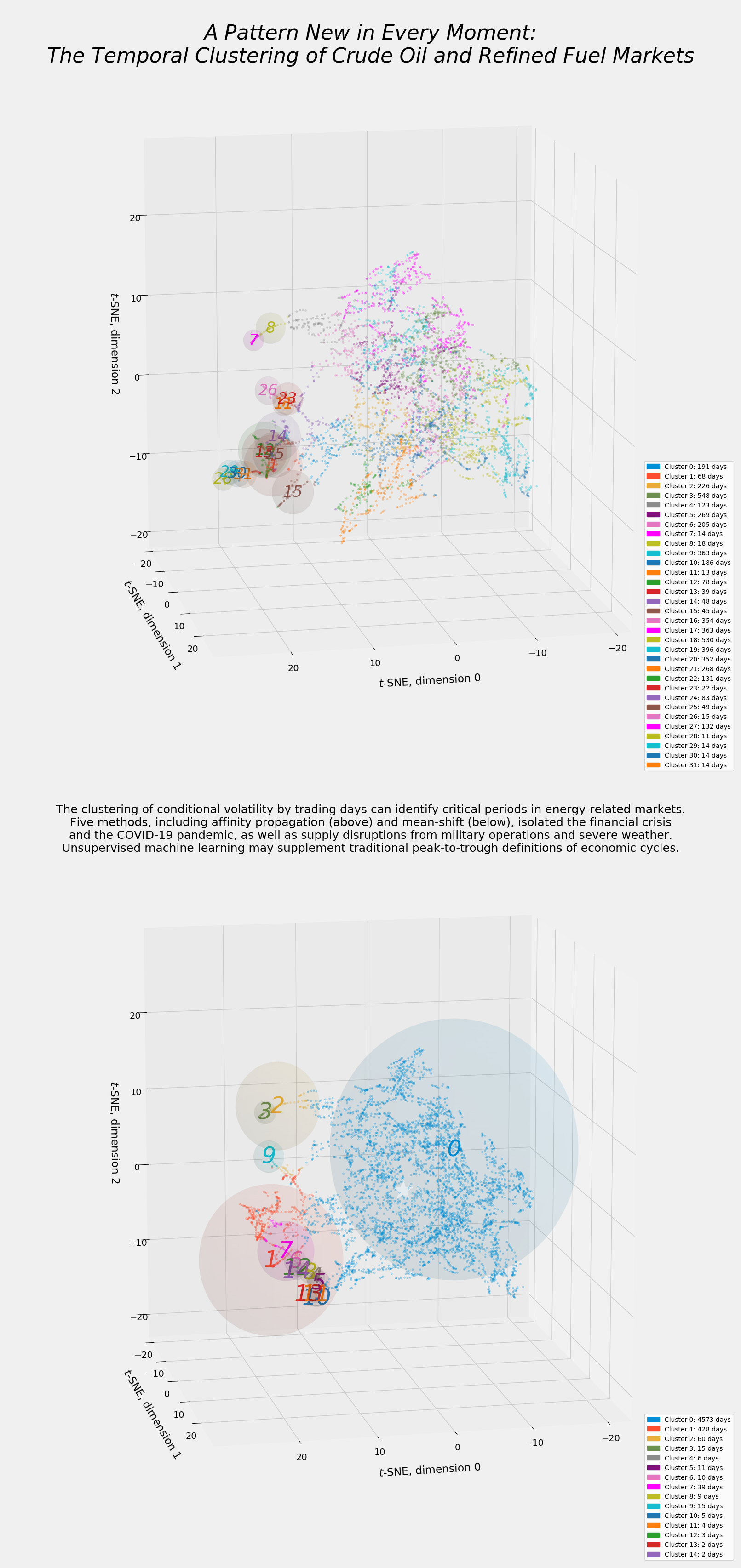
Section 4 aggregates results from five clustering methods—affinity propagation, mean-shift, spectral, k-means, and hierarchical agglomerative clustering—as applied to a comprehensive market basket of 22 commodities and to a more focused basket of four energy-related commodities: Brent, West Texas intermediate, gasoil, and gasoline. t-distributed stochastic neighbor embedding, or t-SNE, helps visualize all clustering results.
Meaningful temporal clusters for broader commodity markets delineate the global financial crisis and the COVID-19 pandemic. Focused clustering in energy-related markets identifies several additional critical periods for crude oil and refined fuel markets. Section 5 presents and distinguishes those two sets of results.
Section 6 discusses the implications of this article’s findings for managers, investors, and policymakers. Critical periods in energy-related markets demand a different approach to hedging and risk management, not merely for commodity investors, but also for investors using commodities to neutralize other sources of risk. The role of energy-related crises in macroeconomic policymaking also warrants careful consideration.
The identification of temporal regimes in commodity markets through clustering suggests the generalizability of unsupervised machine learning to other markets and to macroeconomic data. The second half of Section 6 describes these and other possible paths for future research.
2. Literature Review
The economic literature germane to this article spans four distinct subjects:
- Price volatility in oil and refined fuel markets;
- Comovement and volatility spillovers between these energy-related commodities and other commodity markets;
- Similar connections between energy-related commodity markets, other financial markets, and the real economy;
- Methods for identifying cyclicality and other time-varying effects in commodity markets, stock markets, and the real economy.
This section addresses each body of literature in turn. A review of the relevant literature on unsupervised machine learning is deferred until Section 3′s presentation of materials and methods.
2.1. Price Volatility in Crude Oil and Refined Fuels
2.1.1. Oil Price Volatility
Commodity markets figure prominently in developmental economics and international trade. Representing a quarter of global trade in goods, commodities provide the most important source of income for some of the world’s poorest countries [2,3]. Because advanced economies rely so heavily on petroleum-based fuels for transportation and many industrial processes, the wealth of developed nations also hinges on oil-based commodities [4].
The pervasive financialization of commodities raises the premium on proper understanding of the price and volatility dynamics in these markets [5]. This is particularly true of crude oil and fuels refined from it [6,7,8,9]. Producers and industrial customers have the greatest stake, since oil price volatility directly affects investments in oil inventories, production and transportation facilities, and physical capital based on oil consumption [10]. These sunk investments demonstrate why “costly reversibility” is a prime mover in the economics of market structure and industrial organization [11,12,13,14].
Because of their intrinsic volatility and their dependence on global supply chains, energy markets are especially sensitive to external shocks. The diverse factors affecting oil prices include sociopolitical disturbances, shifts in the global supply and demand, and technological and regulatory changes promoting demand for renewable energy [15]. Discrete events, “such as wars, the release of OPEC production quota decisions, oil stock fluctuations and extreme weather,” also affect oil prices [16] (p. 256).
Chronic or acute, these factors are never stable. Structural breaks punctuate the time-varying conditional heteroskedasticity of oil price volatility [17]. Although conventional tools for forecasting oil prices and volatility abound [18,19], models that ignore structural breaks and other sources of temporal variability in volatility “will have very low power” [17] (p. 555). This is yet another instance in which accurate forecasting relies upon the more realistic assumption that volatility does not remain constant [20].
2.1.2. Refined Fuels: Gasoline and Gasoil (Diesel)
Because gasoline and gasoil are refined petroleum products, their price and volatility dynamics depend heavily upon the economics of oil. These markets are nevertheless subject to forces befitting their proximity to retail consumers. Gasoline and gasoil are affected by time-varying consumer income [21] and the price elasticity of demand for petroleum-based fuels among other retail-level energy sources [22]. Demand for gasoline may be less elastic than typically assumed, especially in the short run [23].
Perhaps the most distinctive trait of the price behavior of refined fuels, particularly gasoline, is its asymmetry [24,25,26,27]. The “rockets and feathers” hypothesis posits that increases in crude oil prices are transmitted much more quickly to gasoline than decreases [28,29,30]. Data across the United States showed that retail gasoline prices increased 0.52 percent within the first week of an anticipated 1 percent increase in oil prices, but fell 0.24 percent within the first week of a 1 percent decrease [31].
Other sources describe asymmetry in gasoline pricing according to Edgeworth price cycles, characterized by sawtooth-shaped time series consisting of many price decreases punctuated by occasional upward jumps [32,33]. Straightforward measurements of gasoline demand have shown that elasticity decreases as volatility rises [34,35]. Both the “rockets and feathers” hypothesis and Edgeworth price cycles are consistent with this account of volatility.
Other sources contest the presence of asymmetry in the relationship between oil and refined fuel markets [36]. Asymmetry, if present for gasoline and gasoil in Europe, is fleeting and appears over very short time horizons [37]. Asymmetry appears in Spain and Italy, but not in Greece, the United Kingdom, or the United States [38]. Time-varying effects such as volatility clustering and structural breaks affect the degree of asymmetry in the transmission of volatility from oil to gasoline [39]. Findings of asymmetry may depend on the frequency at which volatility data is sampled [40].
One study reaches an intriguing conclusion: The “rockets and feathers” hypothesis tells the dominant story of oil–gasoline asymmetry, but not the exclusive story [28]. When oil prices are falling, on average, gasoline prices follow a contrary “boulders and balloons” dynamic by which gasoline more swiftly tracks oil price declines than increases. The reversal in the polarity of oil–gasoline asymmetry strongly suggests that volatility transmission between crude oil and refined fuels varies over time. Indeed, the presence of opposite tendencies, based on the timing of the broader business cycle, suggests that asymmetry, persistence, and cyclicality in volatility must be understood in the context of other capital markets and the macroeconomy [41,42].
Though literature on the price dynamics of gasoil is relatively sparse and inconclusive, national fuel mix policies appear to account for some of this fuel’s differences relative to gasoline [43]. The European Union [44] and the United Kingdom [45] both nudge their transportation sectors to favor gasoil over gasoline. With mixed success, the United States has maintained a heating oil reserve to stabilize prices for this variant of gasoil, widely used to heat homes in the northeastern region of that country [46]. Home heating can be expected to be one of the least elastic sources of demand for gasoil, at least over short time horizons, for households that depend on this fuel.
2.2. Comovement and Volatility Spillovers within Commodity Markets
2.2.1. The Financialization of Commodities and Hedging Strategies
As a prime outgrowth of the coordination of commodity markets with other aspects of global finance [5], comovement and volatility spillovers among commodities warrant careful evaluation [47]. Commodity futures have become popular tools for diversification [48,49]. Tools for managing financial risk in other capital markets apply directly to energy-related commodity markets [50]. Commodities as safe havens can offset turbulence from other asset classes, from equities to currencies [51]. The “universe of financial assets,” spanning diverse “investment strategies,” heightens the importance of “risk transfer between oil” and markets for other “global, large and liquid” assets [52] (p. 56).
Unstable energy prices often induce investors to hold other assets alongside energy commodities. Hedging strategies and portfolio rebalancing enable investors to manage comovement [53]. At a minimum, oil price shocks affect non-energy commodities [54,55,56,57]. A study of volatility in oil and refined fuel should therefore consider comovement and volatility spillovers linking energy with other commodity classes, especially metals and agricultural products.
2.2.2. Precious Metals
The traditional role of precious metals as hedges against inflation and economic turbulence [58] casts those commodities in sharp relief against crude oil and refined fuels [59,60,61]. Markets for oil are more volatile than markets for gold and silver [62]. Precious metals exhibit hedging and safe haven properties vis-à-vis energy [49,59,63,64]. Connections between gold and oil extend to other financial instruments [60,65].
Financial risk may not run equally between two markets. Among instances of volatility spillover in commodity markets [66,67,68], the propensity of oil to transmit volatility to precious metals poses the greatest challenge to investors in energy-related commodities [69,70,71,72]. As the global financial crisis of 2008–2009 demonstrated, precious metal returns may be more sensitive to disaggregated structural oil shocks [72].
2.2.3. Base Metals
Because oil prices heavily affect input costs for industrial processes using base metals, connections between energy markets and metals extend beyond gold, silver, platinum, and palladium [73,74]. Although one study identified platinum, gold, and silver as net transmitters of volatility to oil [60], such spillover may not persist across all periods and market states. Indeed, traditional distinctions between precious and base metals may not hold across all financial conditions. Tin, gold, nickel, lead, and aluminum transmit return and volatility to oil markets. Copper, zinc, and platinum are net receivers—but only “at certain specific moments” [75] (p. 12). Time-varying fluctuations became especially pronounced during the global financial crisis [60] and the COVID-19 pandemic [75].
2.2.4. Agricultural Commodities
Energy markets also transmit volatility to agricultural commodities [3,71,76,77,78,79]. The dependence of agricultural commodity markets on energy prices varies over time [80]. A structural break appears to have shifted the relationship between oil and agricultural commodities after 2006 [81]. Sources differ in attributing the disruption to a change in biofuels policy [76] or to a broader crisis in food crops [78].
The relationship may vary more subtly over time [80]. During periods such as the financial crisis of 2008–2009, oil and agricultural commodity markets crash simultaneously. Connectedness likewise strengthened during the COVID-19 pandemic [82]. Under normal economic conditions, however, these markets move in opposite directions. This pattern implies that hedging will fail in the very conditions when hedges would prove most valuable. The counterbalancing effect also denies investors the opportunity to realize excess profits in both markets.
These conclusions are neither universal nor inevitable. A different study focusing on common crisis periods such as the global financial crisis and the pandemic rejects two key conclusions of other studies [83]. Oil and crops have a bidirectional relationship in which each class of commodities transmits volatility to the other with roughly equal probability over long time horizons. As a surprising consequence, oil and agricultural prices remained relatively stable throughout the pandemic.
Certain crops (particularly corn and soybeans) either compete directly against crude oil as a renewable substitute or serve as a complementary product [84]. A third crop, sugarcane, affects these markets because of its substitutability for corn [85]. Conventional wisdom holds that high oil prices invite competition from corn-based ethanol and soybean-based biodiesel [86].
This relationship, like many others, appears to depend on the state of the market: Spillovers from oil to agricultural and biofuel markets are stronger when oil prices are higher [87]. Conversely, concerns over the diversion of common-pool resources used in agriculture from food to fuel production reach their peak during economic crises [88].
Closer scrutiny of the impact of biofuel policies on oil and gasoline price variability [89] has not found conclusive evidence that energy markets spur volatility in corn [90] or that policy-stimulated demand for biofuels has elevated prices or volatility in agricultural markets [91]. The answer to the conundrum may lie in the limited economic impact of biofuel policies. If such policies were abolished around the world, biofuel demand would implode without materially affecting overall demand for agricultural commodities [92].
2.2.5. The Geopolitics of Energy-Related and Agricultural Commodities
The prominence of oil and export crops in many developing economies heightens the economic, political, and diplomatic sensitivity of volatility spillovers involving those markets [3]. Connectedness between these commodities bridge distant geographic markets, such as Chinese crops and crude oil, whether around the world [93] or specifically in the United States [94]. As a rule, however, research on the impact of oil price volatility on developing countries that import rather than export petroleum remains limited [95].
A global study spanning 157 countries at different stages of development attributed 40 percent of income volatility to oil price fluctuation [96]. Though “the adverse effects of [price] instability” are often “much more severe” in developing countries, those governments can rarely afford “the extensive support programs that typify the agricultural sectors of the developed world” [97] (p. 1729). Dependence on natural resource extraction is so often associated with stunted economic development that this paradox is known as the “resource curse” [98,99,100,101].
Geopolitical tension from oil divides importing and exporting countries [102,103]. Importing countries must rely on insecure foreign sources of an economic lifeblood [104], while global trade and politics drive fiscal policy and economic cycles in exporting countries [105]. The rapid emergence of China portends the revival of a Great Game among global superpowers in central Asia and other oil-rich regions [106].
Again, however, the economic effects are asymmetrical. Economic reactions to energy price shocks in exporting countries are greater and more persistent than in importing countries [107]. In the long run, both oil-importing and -exporting countries stand to lose. At least among OECD countries, oil price volatility stunts economic growth in net importers, while oil price uncertainty hurts net exporters [108]. Furthermore, to the extent that oil price volatility suppresses international trade and globalization, the ensuing reduction of global welfare harms all countries [109].
2.3. Broader Financial and Macroeconomic Effects of Oil and Fuel Price Volatility
2.3.1. Financial Markets beyond Commodities
Oil markets transmit volatility to other capital markets, including equity markets [110,111]. Although one study concludes that the American stock market is neither a net transmitter nor a net receiver of volatility relative to oil or precious metals [60], others have found spillover effects in smaller economies such as Iran [112] and South Korea [113].
Stock returns and stock market volatility in oil-exporting countries such as Qatar, Saudi Arabia, and Venezuela are assuredly affected by oil prices [114]. These effects follow a regime-switching framework based on the cyclical state of these countries’ equity markets—specifically, whether stocks in oil-producing countries are in a bull or bear market [114]. Some sources advise investors in oil-exporting countries to increase their allocation to oil [115,116].
The relationship between oil price volatility and the equity market may depend on the cyclicality of both markets. The “relationship between oil prices and US equities could depend on both the nature of oil price shocks and how well the US stock market is performing” [117] (p. 6). Complete understanding of the mutual dependence of oil prices and broader capital markets requires not only some understanding of cyclicality in commodity and equity markets, but also a principled way of identifying critical periods within financial history.
To like effect, structural heterogeneities in foreign exchange markets coincide with geopolitical and economic impacts [118]. In conjunction with broader macroeconomic phenomena, oil markets exert dynamic influence on trade in currencies [118]. Portfolio management and other forms of risk management therefore hinge on the relationship between oil prices, exchange rates, and the business cycle.
2.3.2. Macroeconomic Effects
Oil price volatility impairs economic growth [119]. Like many other phenomena connected to oil and fuel markets, the macroeconomic effects of disruptions in energy-related markets are asymmetrical. Oil price increases stunt economic growth more deeply than corresponding decreases in price spur economic activity [120,121]. Even sharp price drops may reduce aggregate output in oil-importing countries by raising uncertainty or inducing inefficient reallocation of resources [122].
Macroeconomic uncertainty spurred by oil price volatility varies over time. Volatility typically peaks during financial crises and recessions [123]. Nonlinear measures capture the overall economic effects of oil price shocks [124]. Oil price volatility in the wake of economic, geopolitical, and natural disturbances often combines short-term perturbations with longer-term macroeconomic factors [125].
A useful trichotomy summarizes the macroeconomic component of oil price volatility [126]. First, “most commodity prices are endogenous with respect to the global business cycle” [127] (p. 313). Second, demand shocks cause slow but sustained changes in price. Third, and in stark contrast, supply shocks have immediate but small and ultimately evanescent price impacts. In oil-related markets, crises and recessions generally reduce demand over a sustained period, while geopolitical events and natural disasters tend to disrupt supplies on an acute basis.
This rigidly logical approach to evaluating the macroeconomic effects of oil and fuel price volatility does leave room for potentially exogenous factors to affect uncertainty. Oil “price uncertainty,” conditioned “on macroeconomic uncertainty,” might be a more complete and “suitable measure of uncertainty” than purely volatility-based measures [127] (p. 325). As a matter of broad theory, if not empirical precision, uncertainty may depend more heavily on the predictability of energy-related markets than on their volatility [127].
2.4. Identifying Cyclicality and Critical Periods in Energy Markets, Finance, and the Real Economy
Comprehensive financialization strengthens the connections linking commodities, capital markets, and the broader economy. These relationships reinforce other centrifugal tendencies throughout economics. For instance, asset pricing models should account for tangible assets and human capital as well as financial instruments [128]. The behavior of a firm is likewise influenced by that of its upstream suppliers, downstream purchasers, and competitors in geographically and technologically adjacent markets [129].
Appropriately enough, efforts to track economic cyclicality span stock markets and macroeconomic policymaking. These two domains, neither more than a single degree removed from commodity markets, have invited many efforts to define critical periods. Even though this article applies unsupervised machine language rather than conventional econometric methods, it is motivated by the same desire to trace economic cyclicality in commodity markets, particularly for crude oil and refined fuels.
Stock markets provide the narrower and methodologically simpler basis for comparison. Technical stock analysis typically defines bull and bear markets, respectively, as a market-wide price increase of at least 20 percent since the previous trough or a market-wide decrease of at least 20 percent since the previous peak [130,131,132]. A 10 percent decline is typically described as a “correction” [133]. Designations of bull and bear cycles within market trends can be made only in retrospect, and there is no justification for these arbitrary 10 and 20 percent thresholds beyond the conventions of technical analysis and financial journalism.
For its part, the Business Cycle Dating Committee of the National Bureau for Economic Research (NBER) tracks recessions and recoveries in the United States [134,135,136,137]. The NBER’s methodology relies on a dynamic-factor, Markov-switching model that examines non-farm payroll employment, the index of industrial production, real personal income, and real manufacturing and trade sales [134,136].
Figure 1 describes the NBER’s announcements regarding the arrival and departure of recessions in the United States [138,139]. It depicts smoothed recession probabilities as they rise and ebb. Notably, only two periods from 2000 through 2020 have exceeded 50 percent according to the NBER: the financial crisis of 2008–2009 and the COVID-19 pandemic. The “dot-com” crisis of 2001 approached but did not exceed a 50 percent probability of recession. As is evident in the shaded areas of Figure 1, however, the NBER did define March through November 2001 as a recession.
One can also frame this problem as the mirror image of an event study [140,141]. An event study traces abnormal effects to determine the duration of a suspected market disturbance. Event studies of oil price shocks [142,143], for instance, have evaluated OPEC announcements [144,145] and storms [146]. Conversely, temporal clustering uses economic anomalies to extract events for further examination amid the flow of financial history.
The timing of recession announcements presents an economically significant issue in its own right [147]. By the NBER’s own admission, its business cycle dating committee’s “approach to determining the dates of turning points is retrospective” [148]. Before definitively identifying a peak, “the committee tends to wait to identify a peak until a number of months after it has actually occurred” [148]. Likewise, the committee does not immediately announce a trough. Rather, the committee “waits until it is confident that an expansion is underway” [148].
Under this methodology, announcements of recessions and recoveries are not aligned in time with actual economic activity [149]. In the three decades from 1980 to 2010, “the lag between the determined start of [a] recession” and the NBER’s “peak announcement” has averaged 9 months [150] (p. 645). At a bit more than 15 months, the lag between a trough and its announcement is longer still [150].
The lag between actual macroeconomic phenomena and their announcements creates an opportunity for machine learning, artificial intelligence, and other automated methods for evaluating economic data. For instance, the United States publishes its official Consumer Price Index on a monthly basis, with a delay of several weeks between the gathering of price data by. the Bureau of Labor Statistics and the announcement of each new CPI reading [151]. By contrast, the Massachusetts Institute of Technology’s Billion Prices Project reports a comparable price index on a daily basis [151].
This article develops a methodology for identifying critical periods in energy-related commodity markets. The literature on oil and fuel markets emphasizes volatility and the connectedness of oil and oil-based fuels with other commodities, other financial markets, and the macroeconomy. Instead of defining cycles akin to bull and bear markets or macroeconomic expansions and recessions, this article will try to distinguish between critical and normal periods of trading within markets for petroleum-related commodities. In seeking a crisis-based approach to understanding temporal shifts in these markets, this article aims at an intermediate level of mathematical rigor between the extremes represented by technical definitions of bull and bear markets and the NBER’s recession-and-recovery methodology.
Qualitative distinctions between peaks and troughs, expansionary and recessionary cycles, and critical periods dissolve upon closer mathematical inspection. Critical points in calculus identify points within the domain of a function where the derivative or gradient is zero (assuming that the function is differentiable at those points). Peaks and troughs as maxima and minima constitute critical points in a univariate function. In a multidimensional space representing returns on more than one asset, critical points also include saddle points, where all slopes in orthogonal directions are zero, but no local extremum is attained. In this mathematically informed sense, the methods described and applied in this article cast a wider net than methods dedicated of finding peaks and troughs within a single time series.
The second derivative of logarithmic returns on a financial asset is related to volatility through the Taylor series expansion [152,153]. Points within the domain of a function where the second derivative is zero indicate inflection or undulation. Methods focusing on financial volatility may therefore find inflection and undulation points as well as critical points. These observations are not meant to suggest that this article consciously seeks to find all critical and inflection points in a strictly mathematical sense. Rather, this analogy simply offers a conceptually helpful way of understanding similarities as well as meaningful differences between traditional peak-and-trough approaches and this article’s clustering methods.
As with stock markets and the broader economy, cyclicality in commodity prices has drawn scholarly attention [154]. Efforts to sharpen forecasting and the understanding of the dependence structure in oil and adjacent markets have highlighted differences between normal trading and economic turmoil [155]. The question is whether existing and novel “econometric tools” can generate reliable volatility forecasts when “periods of heightened volatility in crude oil markets are recurrent” [156] (p. 622).
Conventional econometric tools include unit root tests [157,158]. Those tests aided the discovery of structural breaks in 1990 and 2008, coinciding with the first Gulf War and the global financial crisis [17]. Technical analysis inspired by conventional methods for identifying bull and bear cycles in equity markets [159] has aided the search for cyclical effects in oil-based markets, at higher [4] as well as lower frequencies [160].
Computational tools abound amid economic “big data” [151]. Although some sources have mined linguistic [161] and Internet search data [16,162] in search of novel insights, this article uses machine learning and artificial intelligence to answer a more fundamental question: Whether financial economics can detect oil price fluctuation and its impact on the relationship between risk and return [163].
This article applies unsupervised machine learning to conditional volatility in commodity markets over two decades. An ensemble of clustering methods can identify episodes in commodity markets (especially those related to energy) warranting closer examination. Some episodes, particularly the global financial crisis and the COVID-19 pandemic, reflect a broader, more durable demand shock. Other episodes may last mere days. Such acute events should be expected more often within a confined subset of commodities, such as crude oil and refined fuels. These acute events typically involve geopolitical or natural calamities that disrupt supplies of oil and its downstream derivatives.
3. Materials and Methods
3.1. Data
3.1.1. Data Sources and Preprocessing
This article draws its raw data from sources used in [1]. Thomson Reuters’ DataStream provided price data on a range of precious metals, base metals, energy commodities, and agricultural commodities. Specifically, this article relies upon daily prices from 18 September 2000 through 31 July 2020 for gold, silver, platinum, palladium (precious metals); copper, zinc, tin, lead, nickel, aluminum (base metals); Brent, West Texas intermediate crude (WTI), gasoil, gasoline (energy commodities); and palm oil, wheat, corn, soybeans, coffee, cocoa, cotton, and lumber (agricultural commodities).
The preprocessing pipeline took two further steps. Transforming daily prices into continuous logarithmic returns shortened all series by a single day: 18 September 2000. The resulting log return data (as well as the conditional volatility data derived from log returns) therefore covered the period from 19 September 2000 to 31 July 2020. Two additional days were excluded. On 20 April 2020, WTI closed at –37.63. This event rendered it mathematically impossible to calculate the log return for WTI on that day and the next, 21 April 2020. Those two trading dates were also omitted.
The second preprocessing step involved forecasts of conditional volatility from log returns. We calculated the conditional, time-variant volatility for all 22 commodities according to a GJR-GARCH(1, 1, 1) process using Student’s t distribution [1,164]. The mathematical underpinnings of GJR-GARCH(1, 1, 1) have been thoroughly documented [165,166]. GJR-GARCH outperforms alternative time-series models in forecasting financial markets [167].
For purposes of analysis and discussion, we aggregated log return and volatility data according to a precalculated ontology of commodity markets. The vocabulary of commodities trading distinguishes between mined, nonrenewable “hard” commodities (such as metals and fossil fuels) and grown, renewable “soft” commodities [20,88,168,169]. The term “soft” is sometimes reserved for tropical crops such as cocoa, coffee, and sugar [170]. We adopt that narrower definition of “softs” and describe the temperate commodities of wheat, corn, and soybeans as “crops.” Because cotton and lumber span tropical and temperate climates, these commodities can be assigned to either agricultural subcategory. Results from the clustering of log returns support the classification of cotton and lumber as tropical or semitropical softs [1].
These distinctions, paired with traditional divisions among metals and fuels, can be summarized as a traditional ontology of commodities trading:
- Energy (crude oil and refined fuels): Brent, WTI, gasoil, gasoline;
- Precious metals: Gold, silver, platinum, palladium;
- Base metals: Copper, zinc, tin, lead, nickel, aluminum;
- Temperate crops: Wheat, corn, soybeans;
- Tropical and semitropical “softs”: Cocoa, palm oil, coffee, cotton, lumber.
3.1.2. Visualizations of Logarithmic Return and Conditional Volatility Data
This subsection visualizes this article’s core data. Although log return and conditional volatility calculations were performed on all 22 commodities, this article compares only energy-related commodities with one another on an individual basis. This article compares crude oil and refined fuels as an asset class alongside the aggregate categories for metals and agricultural commodities.
Figure 2a depicts cumulative log returns for commodities as asset classes. Relative to other classes, energy-related commodities show many sharper price movements. Figure 2b illustrates cumulative log returns for individual crude oil and fuel markets. Although comovement among individual oil and fuel markets is far tighter (as one should expect) than among broad classes of commodities, sharper upward and downward price spikes, particularly for gasoline, are evident to the naked eye.
Figure 3a,b depict conditional volatility. By analogy to Figure 2a,b, Figure 3a portrays the five broad classes of commodities, while Figure 3b focuses on the four individual energy-related markets. Visibly greater volatility in energy markets dominates Figure 3b. Relative to crude oil markets and even gasoil, the market for gasoline is palpably more volatile. These acute volatility spikes confirm the intuition motivating the conventional exclusion of food and fuel prices from core inflation indices used in the making of macroeconomic policy [171,172,173,174].
3.2. Clustering Methods
3.2.1. General Considerations
Many applications within economics and finance exploit clustering and related forms of unsupervised machine learning [175,176,177,178]. This article applies five clustering methods: Spectral, mean-shift, affinity propagation, k-means, and hierarchical agglomerative clustering. Each of these methods is available in the SciKit-Learn package for Python. The implementation of hierarchical agglomerative clustering in Scipy generated visually distinctive dendrograms for that method.
Previous research had established that temporal clustering should be based on conditional volatility rather than logarithmic returns [1]. All five clustering methods were applied to volatility data arrayed in n rows of trading days and p columns corresponding to the number of distinct commodity markets. For the full volatility array covering all 22 commodities, p = 22. For the energy-specific subarray, p = 4. The two arrays, however, had the same number of trading days: n = 5182.
For both the full 5182 × 22 array and the energy-specific 5182 × 4 subarray, clustering results underwent a crude aggregation inspired by voting classifiers in machine learning [179]. Since clustering of the full 5182 × 22 array reached rough consensus on the financial crisis of 2008–2009 and the COVID-19 pandemic as the two periods of interest, that analysis relied on the union and the intersection of the five sets of clustering results. Using the union of sets is tantamount to allowing a single vote to drive a positive result. The intersection of those sets indicates unanimity. These set theory concepts therefore define the logical extremes of voting methodologies [180,181].
Greater variability in the results for the energy-specific 5182 × 4 subarray required a more flexible approach. For that array, this article aggregated all positive results registered by two or more of the five clustering methods. The most generous voting method, consisting of the union of all positive results, generated a wider range of dates. Though unexamined in this article, those results remain available for future research.
The balance of this subsection will describe each of the five clustering methods.
3.2.2. Spectral Clustering
Spectral clustering operates on a projection of the normalized Laplacian [182,183]. Since this article’s conditional volatility arrays represent 4 or 22 commodity markets as simple functions of a common vector of trading dates, the Laplacian (Δf = ∇2f) is the sum of the partial second derivatives for each of those variables.
Spectral clustering should work very well with financial data. This method exposes individual clusters within highly non-convex structures [184,185]. Since each volatility vector is plotted against the same vector of trading dates, the resulting arrays of volatility forecasts by date are tantamount to overlapping curves on a two-dimensional plane. Spectral clustering therefore excels precisely where conventional statistical measures of central tendency and variability fail to describe the shape of the data to be clustered.
These properties have made spectral clustering especially popular in computer vision and image processing [186,187]. The ability of spectral clustering to detect blobs and edges suggests potential success with economic time series. In mathematical terms, image and time-series data are quite similar. Unlike documents that have been vectorized for natural language processing, these data sources consist of perfectly dense arrays whose columns observe the same scale, or at least nearly so. Still images and simple, harmonized arrays of economic time series can be rendered in a nominally two-dimensional format.
Spectral clustering generated the fewest discrete clusters. Consequently, the spectral method may be regarded as setting the most conservative clustering baseline.
3.2.3. Mean-Shift Clustering
An extension of more traditional pattern-recognition algorithms, mean-shift clustering uses nonparametric techniques to identify deviant blobs in an otherwise smooth space [188]. Alongside k-means, mean-shift is one of two centroid-based methods in this article. The distinctive process that gives mean-shift its name relies on a recursive updating of potential centroids that would represent the mean of the points within a given region. A final postprocessing stage eliminates near-duplicates before reporting the final list of centroids. Hybridizing the mean-shift method with agglomeration can reduce the computation cost of mean-shift clustering [189].
3.2.4. Hierarchical Agglomerative Clustering
Hierarchical clustering methods decompose and arrange mathematical objects according to dendrograms, or trees expressing phylogenetic relationships [190,191,192]. The agglomerative method begins from the “bottom” of a dataset and combines instances into clusters until all data has been assigned to a single, overarching cluster [193].
Bottom-up agglomeration is less computationally demanding than top-down division [194,195]. Four methods for computing distances in hierarchical clustering are widely used: Ward’s method and single-, average-, and complete-linkage [196,197,198,199].
In economics and finance, hierarchical clustering has evaluated stock markets [200,201], buildings and real estate [202,203], broader financial indicators [204], and the relationship between financial markets and the real economy [177]. Hierarchical clustering of cryptocurrency markets [205] intensifies the urgency of research into this asset class during market turbulence [206].
One source has used hierarchical clustering to identify correlation patterns similar enough to comprise distinct market states [207]. Aside from our own work [1] and the use of multidimensional scaling to evaluate comovement among commodities during subjectively defined crises [164], this application of hierarchical clustering represents the most extensive effort to classify periods in financial history through unsupervised machine learning.
3.2.5. Affinity Propagation
Affinity propagation identifies typical cluster members by exchanging quantitative messages between data pairs until the algorithm converges on a high-quality set of exemplars [208,209,210]. This property distinguishes affinity propagation from mean-shift and k-means clustering, which are centroid-based methods.
Under SciKit-Learn’s default settings, however, affinity propagation generates far too many distinct exemplars. To the extent that other methods (specifically spectral, mean-shift, and hierarchical clustering) can better estimate the optimal number of clusters, an instance of affinity propagation can alter the element preference from its default value of the median of the array of input similarities [211]. To a limited extent, this adjustment enables affinity propagation to alter the number of clusters that it finds.
Affinity propagation spans an impressive range of applications. Affinity propagation is used to cluster microarray and gene expression data [212,213,214] and in sequence analysis [215]. Applications beyond bioinformatics [216] include natural language processing [217,218,219] and computer vision [220,221]. Especially if calibrated so that element preference yields something close to the optimal number of exemplars, this versatile clustering method should accommodate financial time series.
3.2.6. k-Means Clustering
One of the oldest clustering algorithms [222], k-means clustering remains a popular way to partition mathematical space [223]. k-means clustering excels in detecting fraud [224] and firms at risk of default or failure [225]. Other financial applications include the forecasting of returns and the management of investment risk [176,226,227,228]. Our own previous research on commodity markets relied heavily on k-means clustering [1].
k-means clustering does require more careful handling. More than other methods, k-means clustering depends on algorithms for determining the ideal number of clusters [229,230]. In addition to k, the optimal number of clusters, this centroid-based method depends entirely on randomized instantiation [231]. To ensure replicability of results, this article seeded SciKit-Learn’s pseudo-random number generator with the value of 1. Finally, k-means clustering cannot detect objects lacking a hyper-ellipsoidal shape [232].
3.3. t-Distributed Stochastic Neighbor Embedding (t-SNE)
This article uses a single method of manifold learning: t-distributed stochastic neighbor embedding, or t-SNE [233,234,235]. t-SNE reduces distances between similar instances and maintains distances between dissimilar instances. Although this article applies t-SNE solely for visualization, t-SNE can be a valuable form of unsupervised learning on its own. Preprocessing with t-SNE can detect and remove outliers in preparation for the application of convolutional neural networks to computer vision [236].
4. Results, Part 1: Temporal Clustering
Clustering results differ dramatically according to the underlying array of conditional volatility forecasts. This section accordingly separates results for the full 5182 × 22 array of all commodities from results based on the smaller 5182 × 4 energy-specific array.
Differences among clustering methods are also stark. Clustering differs from classification through supervised machine learning in a crucial respect. Clustering results do not correspond to a priori labels assigned by a human. Analyst judgment therefore plays a subtler role. Each clustering method must be evaluated on its own terms. Moreover, each method’s results must be evaluated in light of all others and against the backdrop of unavoidably subjective judgment. Each method’s underlying mathematics, however, offers principled guidance on the exercise of that discretion.
4.1. Temporal Clustering of the Full Array of Conditional Volatility Forecasts
4.1.1. The Naïve Biennial Baseline
The naive clustering of all 20 years of commodities trading data provides a valuable starting point. Consider the possibility that a fixed and predetermined period of time should define each segment of financial interest. This hypothetical is far from absurd; monthly, quarterly, or annual reporting slices financial time in precisely this way. In the interest of convenience, we select intervals of two calendar years each.
Figure 4 establishes a visual baseline for all temporal clustering. Consistent reliance on t-SNE to reduce all 22 dimensions produces a uniform three-dimensional projection of conditional volatility forecasts. Synthetic centroids generated by the average of all observations for each biennium supply a rough sense of those two years.
Cluster 9 is particularly interesting because the 2019–2020 biennium includes the global maximum for cumulative log returns on precious metals and the global minimum in cumulative log returns on oil and fuels. That cluster’s synthetic centroid falls very near the global center. Its corresponding observations, in cyan, stretch across the financial firmament, as measured by its width across the zeroth t-SNE dimension.
Expanding all spheres from Figure 4 and Figure 5 reveals the futility of arbitrary biennial clusters. If spherical radii corresponding to each cluster define the mean distance of each observation from its corresponding synthetic centroid, then the size of each sphere and its overlap with other spheres suggest the extent to which each cluster is internally cogent and externally distinct. Internal cogency, if present, should reveal itself through contiguous or nearly contiguous clusters in an ordered, one-dimensional projection along a temporal axis. An ordered, horizontal representation would indeed display 10 perfectly contiguous, nonoverlapping clusters. That is an artifact of the arbitrary definition of those clusters, however, and not any mathematical property captured by t-SNE.
4.1.2. Spectral Clustering
Spectral clustering of all conditional volatility forecasts identifies eight clusters. Although this method does not generate centroids, finding the mean of each cluster’s members in the three-dimensional t-SNE manifold produces synthetic centroids.
Figure 6 reveals the complete t-SNE manifold of spectral clusters. Clusters 1, 2, 3, and 5 appear in a tight group at upper left. Clusters 1 and 2 contain only two days each, while cluster 3 adds only nine more. The tiny size of these clusters is implied by their compactness.
Two other groupings also stand out. Clusters 4 and 7 occupy the lower foreground. Cluster 6 stands alone. As with clusters 1, 2, and 3, a tight radius implies that cluster 6 consists of a small number of days. Indeed, cluster 6 contains only 22 days.
The vast majority of trading days—4920 out of 5182—belong to cluster 0. The t-SNE manifold suggests that cluster 0 may be the fallback cluster representing ordinary trading days, when volatility levels do not substantially deviate from their central tendency.
The most useful representation of temporal clusters, of course, is the one plotted against the ordered vector of dates. Figure 7 reveals how the eight spectral clusters almost perfectly identify two critical periods of interest from 2000 to 2020. The height of the bars communicates categorical rather than ordinal or numerical information. Because of the fortuity that spectral clustering assigned the number 0 to the default, catch-all category, all clusters numbered 1 and above identify periods of interest.
Spectral clustering identified the financial crisis of 2008–2009 and the COVID-19 pandemic. Almost miraculously, six of the remaining seven clusters are perfectly contiguous. Instances from cluster 5, though split by clusters 1, 2, and 3, joined those other clusters to form a continuum covering the beginning of the pandemic. Cluster 6 covers the final 22 days in the dataset. Whether those days belong with the earliest phase of the pandemic or instead indicate a transition toward noncritical cluster 0 may be inferred from the location of cluster 6 in Figure 6 as well as the statistical summary of each cluster.
The resolution of Figure 7, however, is not sharp enough to reveal additional insights. Cluster 5 consists of two subclusters separated by nearly 19 years. The earliest instances in cluster 5 occur in 25–28 September 2001, exactly two weeks after the terrorist attacks of 11 September 2001. The remaining 67 days in cluster 5 started in March 2020, coinciding with the outbreak of COVID-19 in Europe and North America. This represents evidence, however faint, that an event unequivocally related to energy markets might sway the commodities market as a whole.
4.1.3. Mean-Shift Clustering
Mean-shift clustering generated results remarkably similar to spectral clustering. In certain respects, mean-shift clustering might be even more parsimonious.
Figure 8 identifies two periods of potential interest: The tight clump formed by clusters 2, 4, and 5 at left and the looser pair of clusters 1 and 3 at bottom. Because t-SNE manifolds are shaped by their underlying data, Figure 8 can be compared directly with other t-SNE manifolds. Figure 4, Figure 5 and Figure 6 make it apparent that clusters 2, 4, and 5 correspond to COVID-19, while clusters 1 and 3 track the financial crisis of 2008–2009.
The ordered timeline in Figure 9 confirms these intuitions. Clusters 2, 4, and 5 indeed cover the COVID-19 pandemic. Notably, the final 39 trading days (9 June through 31 July 2021) fall within cluster 0. Mean-shift results suggest that the final 22 days might be better classified as “ordinary” trading days rather than part of the COVID-19 crisis.
4.1.4. Hierarchical Agglomerative Clustering
The visual signature of hierarchical clustering is the dendrogram. The dendrogram has the added benefit of offering principled guidance on the optimal number of clusters.
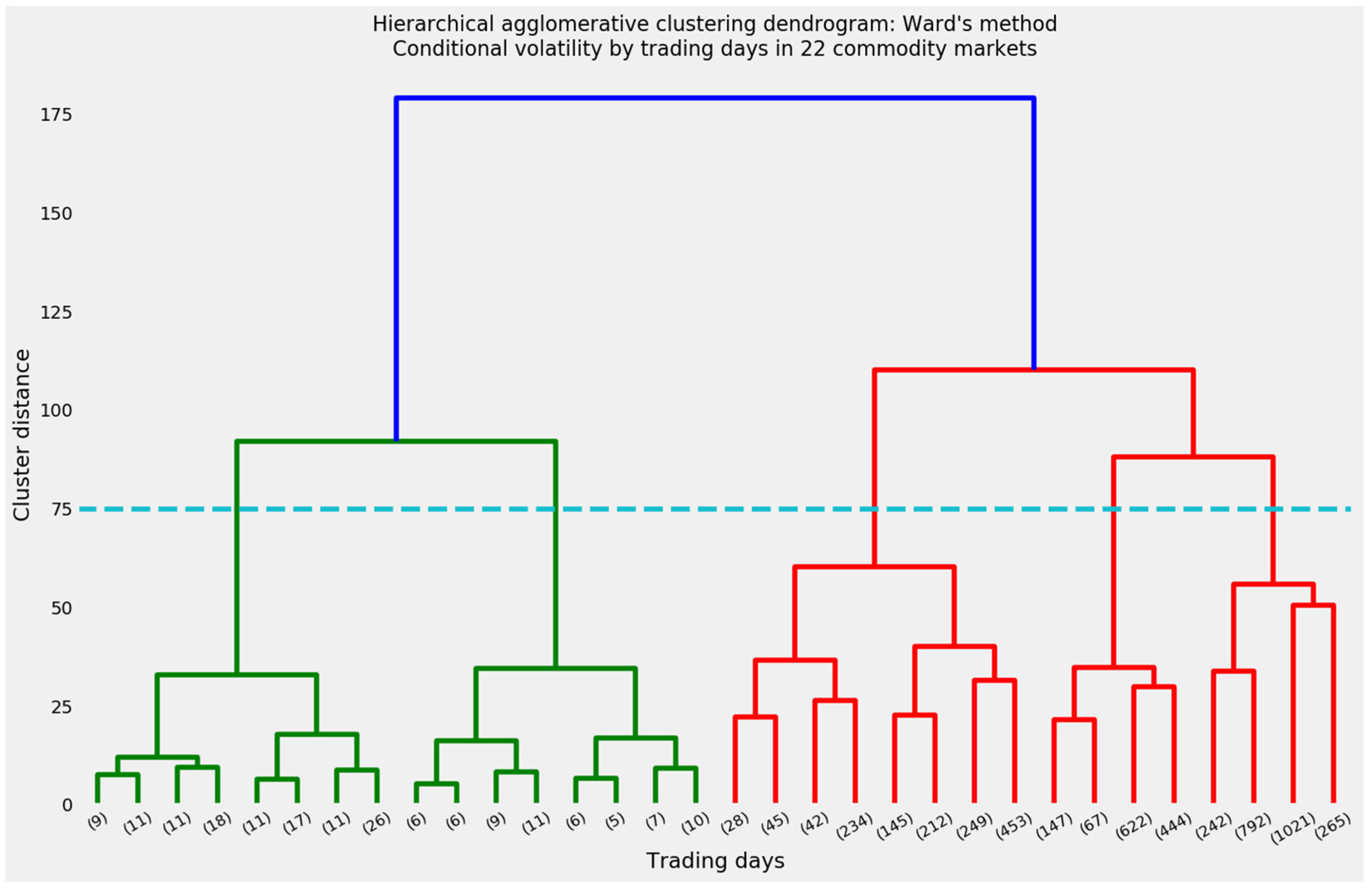
Figure 10 displays the dendrogram for hierarchical agglomerative clustering using Ward’s method and Euclidean distances. The height of the branches offers guidance on the ideal number of clusters. In principle, the ideal number of hierarchical clusters may be as low as two. The height of the blue branches exceeds the vertical distance between any other set of splits. Splitting this dataset into two temporal clusters is tantamount to the binary classification between crises and ordinary (or non-critical) periods.
The dotted horizontal line in Figure 10 intersects five vertical branches. The comfortable vertical distance on either side of 75 implies that 5 is a near-optimal number, if we are unwilling to abandon multiclass in favor of binary clustering. In any event, the logic of agglomeration makes it easy to rearrange the five clusters as two.
Hierarchical agglomerative clustering in Python can designate an arbitrary number of clusters, k ∈ [1, n]. Having determined k = 5, we can project the t-SNE manifold in three dimensions as well as the ordered timeline.
The three-dimensional t-SNE manifold of hierarchical clustering results differs in striking ways from its spectral and mean-shift counterparts. Figure 11 divides noncritical trading days more evenly among three clusters: 0, 1, and 2. Clusters 3 and 4 are the outliers. Cluster 3 surely represents the financial crisis, while cluster 4 captures COVID-19.
The ordered timeline in Figure 12 confirms the intuitive interpretation of the t-SNE manifold. Again, departures from ordinary trading are designated by higher-numbered clusters. The spike for cluster 3 coincides with the financial crisis, while cluster 4 rises during the COVID-19 pandemic.
4.1.5. Affinity Propagation
The final two clustering methods, affinity propagation and k-means clustering, require more computation and discretionary judgment. These difficulties arise from a simple difference: Default settings for affinity propagation and k-means clustering generate a larger number of smaller clusters. Worse, many of those clusters cover non-consecutive days, despite their relatively small size.
Adjusting the element preference matrix enables affinity propagation to generate a desired number of exemplars. This trait of affinity propagation is not infinitely elastic. Nevertheless, a simple matrix of element preferences generated five clusters, the same value of k in hierarchical agglomerative clustering. Those element preferences consisted of the median (not mean) of each vector of volatility forecasts, uniformly scaled by −3000.
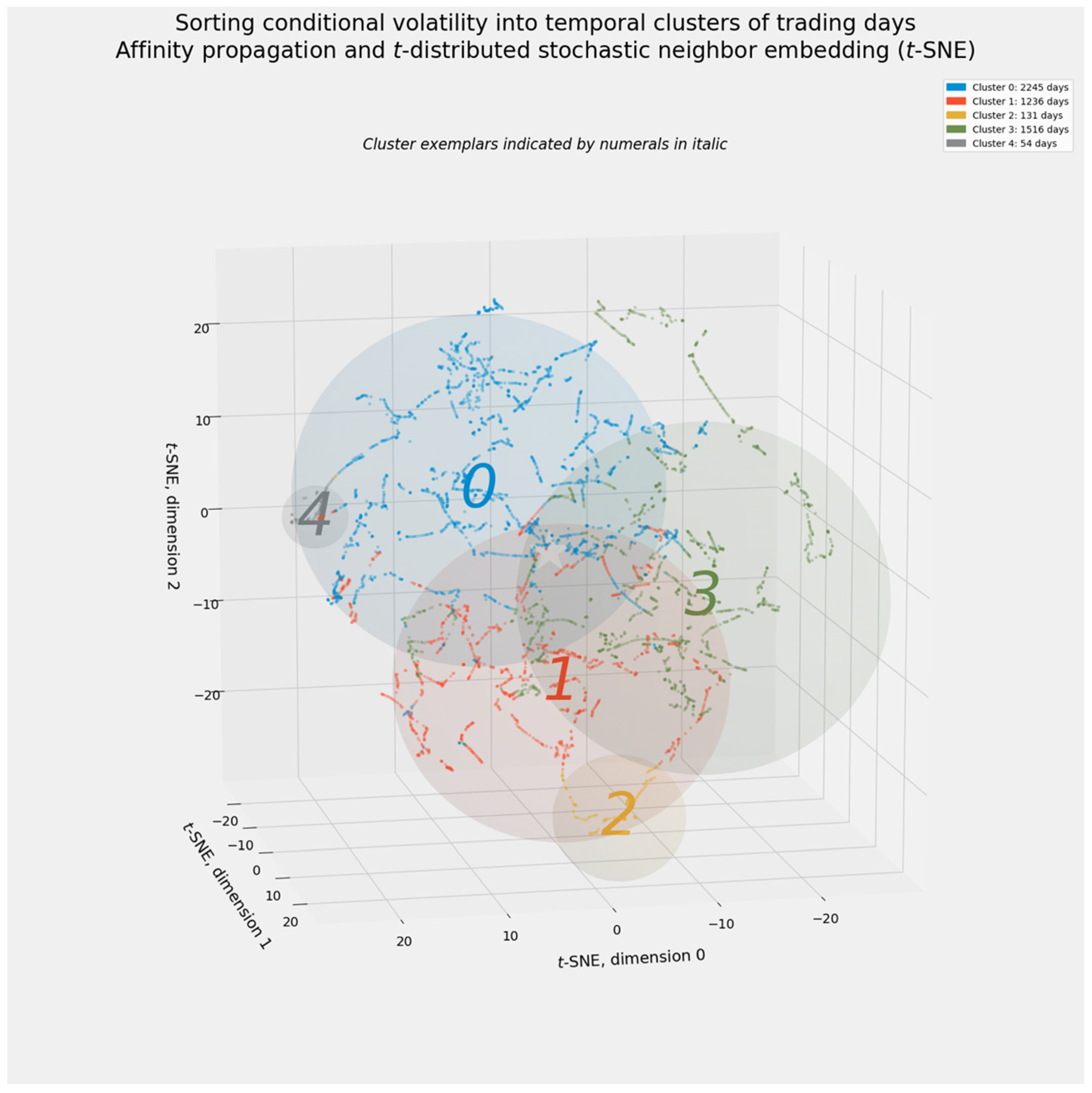
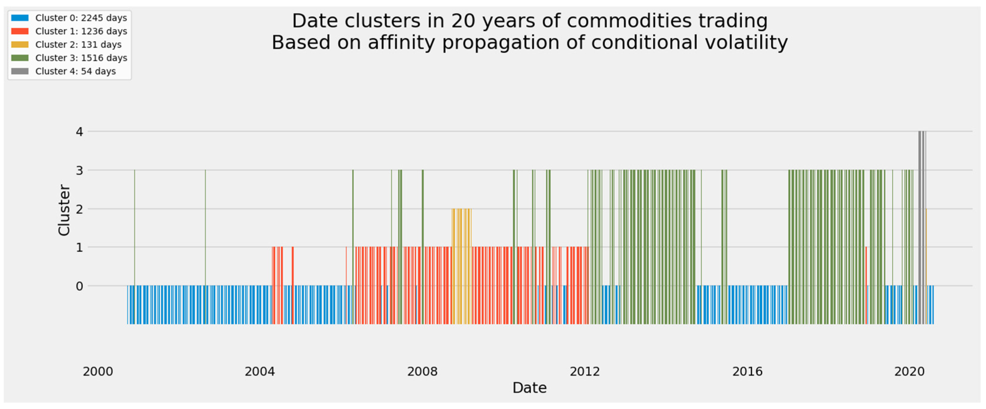
Figure 13 shows how closely affinity propagation, once nudged toward five clusters, resembles hierarchical agglomerative clustering. Critical days appear in clusters 2 and 4, which respectively define the financial crisis and the pandemic.
Figure 14 places these clusters within an ordered timeline. Cluster 2, however, covers not only the financial crisis of 2008–2009 but also the three days immediately following cluster 4′s definition of the pandemic. Consistent with other clustering results, this minor deviation from perfect contiguity suggests that volatility during the COVID-19 crisis drifted toward conditions characterizing the longer-lasting “great recession.”
4.1.6. k-Means Clustering
This article’s exercise in k-means clustering on all conditional volatility forecasts duplicates the temporal clustering in [1], with a salient difference: The value of k, now fixed at six, is the average number of clusters found by other methods (Figure 15). Conventional methods for optimizing k did not prove particularly satisfying. It remains possible to determine k through other clustering methods.
Like mean-shift clustering, k-means clustering relies on the stochastic instantiation of centroids. k-means clustering, however, generates the least contiguous and the least visibly cogent set of clusters. Figure 16 reveals only two wholly contiguous clusters (1 and 4), which coincide with the financial crisis and the pandemic.
4.1.7. The Union and Intersection of Clustering Results for the Full Volatility Array
Though similar, these five clustering methods differ subtly, just enough to require human intervention. Some methods confine all results for the financial crisis or the pandemic to a single cluster. Others divide results among as many as four clusters. Affinity propagation associated three days after its COVID cluster with the earlier financial crisis.
Prior intuitions about any particular clustering method are just that: prior intuitions. The “no-free-lunch” theorem of machine learning posits that no single method can be expected to outperform others in every task [237]. Moreover, machine-learning ensembles typically outperform any individual model [238]. Some method of aggregating results from different clustering models seems advisable.
Elementary set theory provides a simple solution. The union of all clustering results identifies a critical period as long as any method assigns a date to a critical period. The intersection of those results demands agreement among all methods. Given the simplicity of finding agreement over exactly two periods—the financial crisis and the pandemic—these opposite extremes of any plausible voting algorithm define the range of answers.
Figure 17 depicts this simple voting algorithm’s parsimonious results. The union of all results defines the financial crisis as 16 September 2008 to 24 April 2009. The intersection of those results narrows the timeframe so that it runs from 16 October 2008 to 17 March 2009.
The definition of the COVID-19 pandemic is likewise perfectly contiguous by either criterion. The union of results defines the COVID crisis as 10 March to 1 July 2020. The narrower intersection of those sets also begins on 10 March but ends on 26 May 2020.
4.2. Temporal Clustering of the Energy-Specific Array of Conditional Volatility Forecasts
We now apply all five clustering methods to the energy-specific 5182 × 4 subarray of conditional volatility forecasts. The smaller size of this array nudges all methods toward finding more clusters. That property makes some clustering models more difficult to manage. On the other hand, the relative stability of clustering on the grand array of 22 commodities suggests that this suite of unsupervised machine-learning methods can be successfully extended to larger financial markets (including equity markets with hundreds or thousands of stocks) and to arrays of macroeconomic indicators.
Dispensing with the naïve clustering of observations by arbitrary two-year periods, we begin with spectral clustering and progress through all other methods.
4.2.1. Spectral Clustering
Figure 18 reports spectral clustering results for the time periods within the subarray of energy-specific conditional volatility.
On the energy-specific subarray, as with the full array, spectral clustering is a very conservative method. It finds fewer and smaller clusters apart from a single large cluster of ordinary observations. In Figure 18, clusters 1 through 6 adhere together during the COVID-19 pandemic. Cluster 7 stands apart in time and contains 17 consecutive trading days. Cluster 0 accounts for nearly 99 percent of the full 5182 days.
Figure 19′s ordered timeline reveals that cluster 7 does not overlap any period associated with the financial crisis of 2008–2009. Rather, cluster 7 consists of 17 days in August and September 2005. This is the first energy-specific event not identified by the broader array of all commodities. As will become apparent, these days coincided with Hurricane Katrina, which profoundly affected oil production and gasoline refining in and near the Gulf of Mexico [239,240]. Indeed, an enduring structural break between crude oil and spot gasoline prices is attributed to this event [241].
4.2.2. Mean-Shift Clustering
Relative to spectral clustering, the mean-shift method finds nearly twice as many clusters. More intriguingly, mean-shift clusters deviating from the central tendency of energy-specific volatility gather on a single side of the three-dimensional t-SNE manifold.
Figure 20 shows how mean-shift clustering is based on centroids. The centroids indicated by numerals are visibly distinct from the apparent center of gravity for each cluster within the t-SNE manifold’s stylized three-dimensional space. Clusters 0 and 1, the two largest, exhibit the greatest apparent dislocation between centroids and individual instances. All other clusters, except perhaps clusters 2 and 7, are more likely to identify brief, compact events in the trading in crude oil and refined fuels. Such events likely arise from supply disruptions, as opposed to longer-lasting shifts in demand associated with broader crises affecting all commodities.
Figure 21 renders mean-shift results on an ordered timeline. Mean-shift clustering is manifestly more sensitive than spectral clustering. Cluster 0 plays its usual role as the fallback category. All clusters numbered higher than 1 are much smaller, containing (in two instances) as few as two days. Pronounced spikes are associated with the global financial crisis and the pandemic, as well as a previously undetected 2016 event.
Clusters 1 and 2, as the second- and third-largest clusters among the 15, fall between the extremes represented by cluster 0 and collectively by clusters 3 through 14. In addition to indicating several periods in the early 2000s, Cluster 1 brackets better known, already identified volatility events. It may be reasonably surmised that this cluster indicates the beginning or the end of distinctive events. Its appearance at the end of the peak of the pandemic reinforces what all-commodity clustering has already suggested: The pandemic arrived suddenly and began to relax almost as quickly.
Cluster 2 recurs on multiple occasions in the first half of this 20-year period and again in 2015. Those 60 trading days should share characteristics that distinguish them from the financial crisis, the 2016 event, and the pandemic.
Recombining mean-shift clusters from 15 into four—0, 1, 2, and all clusters numbered 3 or higher—provides a clearer picture. Figure 22 reports this summarized timeline.
4.2.3. Hierarchical Agglomerative Clustering
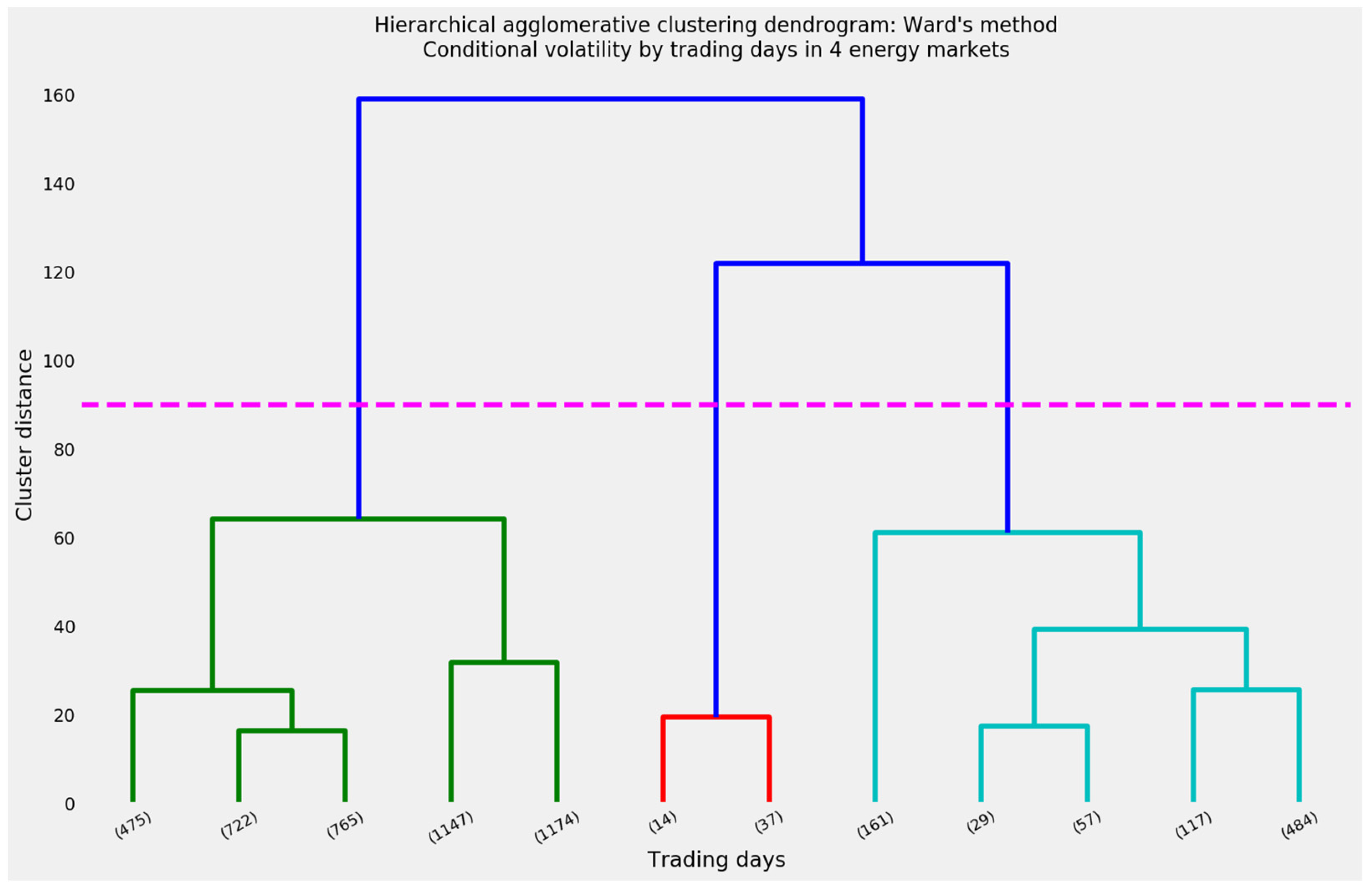
As a matter of visual interpretability as well as mathematical logic, hierarchical clustering begins with a dendrogram. Figure 23 suggests that the ideal number of clusters may be as low as three: A concentrated cluster of 51 trading days (not necessarily consecutive) in the middle in red, a moderately large supercluster of 848 days at right in cyan, and a very large supercluster of the remaining 4283 days at left in green. Deviating from cluster distance as a guide to the optimal value of k yields the 12 clusters along the bottom.
Distances within these 12 clusters average less than 30, as opposed to the distance of 60 separating a three-cluster configuration from its five-cluster alternative. Even so, many of these clusters will exhibit so little contiguity that it will take considerably more analyst judgment to cogently interpret hierarchical clustering.
The t-SNE manifold of hierarchical clustering in Figure 24 looks decidedly unlike the manifolds for spectral and mean-shift clustering. The affinity propagation and k-means manifolds will exhibit a shape similar to the hierarchical results. The greatest difference lies in the relative sizes and overlapping locations of the spheres representing the clusters. Aside from clusters 9, 2, 10, and perhaps 5, these clusters have large radii and overlap their neighbors. The centroids are synthetic, as in spectral clustering, and not stochastically instantiated, as in k-means. Overlapping spheres suggest that the adjoining clusters will not be perfectly contiguous, or even close to being so.
The ordered timeline in Figure 25 confirms these fears. Cluster 0, the closest representation of normal trading, has shorter stretches of uninterrupted, contiguous cogency than the default, background trading clusters under the spectral or mean-shift methods. Cluster 1, which appears during the financial crisis and the pandemic, also appears in 2001. Reducing the total number of clusters below the 15 clusters generated by mean-shift did not bring visible order to the timeline. Additional analyst judgment seems advisable.
Figure 26, the revised manifold, highlights the six smallest hierarchical clusters. A principled case can be made to include cluster 8, the seventh smallest among 12, because of its proximity to cluster 5 in the t-SNE manifold and in Figure 23′s dendrogram. On the other hand, cluster 8 adds 484 days to the 415 total days in clusters 1, 2, 5, 7, 9, and 10. At 415 total days, those clusters comprise almost exactly 8 percent of the 5182 trading days. Adding 484 days from cluster 8 would raise the share of critical trading days to more than 17 percent. For the sake of comparison, mean-shift clustering identified 609 trading days of interest, while spectral clustering found only 70.
Whether critical periods in energy commodity trading comprise 8 or 17 percent of an entire timeframe requires delicate analyst judgment. An incidental benefit of forecasting conditional volatility through GARCH is the ability to estimate the degrees of freedom for the t-distribution that best fits each series of returns. Figure 27 shows that the estimated degrees of freedom for energy-related commodities ranged between 3.03 (WTI) and 3.71 (gasoil). For an equally weighted market basket of oils and refined fuels, ν ≈ 3.51.
The degrees of freedom estimate enables the cumulative distribution function for Student’s t-distribution with location = 0 and scale = 1 to describe the size of the tails at a given value of ν. At this dataset’s estimates for ν, the two-tailed estimate for F(x | |x| > 2) ranges from 0.121634 for gasoil to 0.138395 for WTI. The estimate is 0.125950 for the equally weighted market basket. The one-tailed estimate would be exactly half of those values. The one-tailed estimate for F(x | x > 2) might be justified on the reasoning that volatility is invariably non-negative and that outliers found through clustering are likely to exhibit extremely high rather than extremely low volatility. That rationale, to say nothing of methodological conservatism, supports a smaller number of clusters.
By either measure, the six or seven smallest clusters occupy a distinct edge within Figure 26. All of the candidate clusters lie a palpable distance from the t-SNE manifold’s center of gravity. This is intriguing (if not altogether conclusive) visual evidence that a size-based criterion can successfully isolate outliers among trading days.
Figure 28 simplifies the ordered timeline in Figure 25 by reducing the more conservative six-cluster interpretation of hierarchical clustering into binary classification. Those six clusters have been aggregated into a single “critical” supercluster, while all other days are classified as a normal, noncritical background. In addition to the financial crisis and the pandemic, simplified hierarchical clustering identifies periods of interest in 2000, 2001, 2003, 2005, 2015, and 2016.
4.2.4. Affinity Propagation
The smaller size of the energy-specific subarray created immense difficulty with affinity propagation. Scaling the element preference matrix according to the median values for each series cannot reduce the number of clusters close to the range of eight to 15, the number of clusters found by the spectral and mean-shift methods. More aggressive efforts prevented the algorithm from converging. The smallest number of viable clusters in affinity propagation appears to be 32.
Affinity propagation generates a beautiful but deadly t-SNE manifold (Figure 29). The large number of overlapping clusters, many enveloped in spheres with moderate to large radii, suggests that this method yields highly atomized, noncontiguous clusters.
Figure 30 displays an ordered timeline whose clusters are extremely hard to interpret. Affinity propagation is even more chaotic than hierarchical clustering (Figure 25). The larger the number of clusters, the likelier that individual clusters will splinter internally. Identifying financially meaningful groups of trading days requires extensive work.
Experience with more tractable clustering methods suggests a way forward. Critical and ordinary trading days are not uniformly distributed. The very process used to forecast volatility—GJR(1, 1, 1)-GARCH—presumes heteroskedasticity in the sequence of logarithmic returns. All else being equal, clusters identifying extreme levels of volatility are likely to be smaller than clusters describing lower background levels.
A viable filter therefore consists of tagging affinity propagation clusters for further evaluation until the cumulative number of trading days reaches a certain threshold. The 415 out of 5182 days selected by hierarchical clustering provide a workable benchmark. Isolating the 14 smallest among 32 clusters yields 384 trading days, roughly 7.4 percent of the total. Adding a 15th cluster would add the 78 days from cluster 12 and raise the number of potentially critical days to 459, or nearly 8.9 percent. Because cluster 12 is so close to the 14 even smaller clusters, we included it. Fortuitously, that choice ultimately made no difference in aggregation through voting.
Figure 31 isolates the 15 smallest affinity propagation clusters. As expected, these clusters occupy the left edge of the t-SNE manifold and resemble the critical clusters chosen by hierarchical clustering (Figure 26). Four subgroups are evident: Two appear closer to the top: Clusters 7 and 8 in one supercluster and clusters 11, 23, and 26 in another beneath it. Clusters 28 through 31 occupy the far upper left. Finally, clusters 1, 12 through 15, and 25 comprise a more diffuse but still distinct supercluster at lower left.
Figure 32 isolates these four superclusters. The first three superclusters cover contiguous or nearly contiguous periods corresponding to energy-trading events in 2005, 2016, and 2020. The last of these plainly covers the COVID-19 pandemic—specifically, its frantic first weeks. Clusters in 2005 and 2016, wholly distinct from the financial crisis and the pandemic, imply the occurrence of events quantitatively distinct from the fourth supercluster. Those clusters unite several events in the early 2000s and the back half of the pandemic with the financial crisis.
Analyst judgment, aided by the heuristic tool of choosing the k smallest clusters until some fraction of all trading days is attained, rescued an initially frustrating set of results from affinity propagation. We will apply a similar approach to k-means clustering.
4.2.5. k-Means Clustering
Finding the optimal number of clusters is as difficult as it is pivotal for k-means clustering [229,230]. Other methods have yielded as few as eight and as many as 32 clusters. Without reliable guidance from other tests, we proceed with k = 12, as suggested by hierarchical clustering and roughly halfway between spectral and mean-shift clustering.
Figure 33 shows another treacherously beautiful, highly overlapping set of clusters. Although k-means clustering proceeded on a value of k akin to the number of clusters found by mean-shift and hierarchical clustering, it attains less clarity. The failure to deliver cogent clusters vexed affinity propagation and ultimately required considerable human intervention. Finally, the radial sizes of the spheres within the t-SNE manifold, aside from clusters 2, 6, 10, and maybe 11, suggest that few if any clusters will be close to contiguous.
As expected, Figure 34 shows a deeply fractured k-means timeline. Only clusters 6 and 10 approached perfect contiguity. Cluster 10 is more readily associated with the COVID-19 pandemic. Cluster 6 identifies the September 2005 Katrina event, which eluded detection by temporal clustering of all commodities.
The previously deployed size-based filtering technique converts the superficial chaos of k-means clustering into a credible division of energy-trading history. Figure 35 isolates the six smallest clusters (2, 6, 10, 11, 8, and 0) at the familiar left edge of the t-SNE manifold.
Figure 36 reduces the apparent chaos in k-means clustering (Figure 34) into a binary indicator of critical events. Familiar episodes have emerged: In addition to the financial crisis and the pandemic, k-means clustering isolates events in the early 2000s (including August/September 2005) as well as events in 2015 and 2016.
4.2.6. Aggregating Clustering Results through Voting
All that remains is the aggregation of clustering results through voting. The much smaller number of energy-related commodities makes clustering more sensitive and more likely to find a larger number of critical events. In addition, spectral clustering is much more conservative than other methods. Consequently, some gradations in addition to the extreme outcomes of set theory might be warranted.
The union of all sets of clustering results is tantamount to a one-vote regime. The intersection of those sets effectively imposes a unanimous hard voting regime. Tabulating positive results from each clustering method as a single, equally weighted vote facilitates as many gradations as there are models. In this instance, five distinct models can generate votes ranging from 0 to 5. Any positive result is an element of the union of all five sets. The more votes required, the more stringent the voting regime becomes, until the intersection of all sets reaches the extreme of unanimity.
Figure 37 displays voting results. The only trading days receiving a single vote were those identified by mean-shift clustering but by no other method. Aggregation through voting becomes most interesting at the threshold of two votes. Moreover, the 70 days receiving unanimous support are coextensive with the days found by spectral clustering. Of the other 400 days, 333 received unanimous support from the four remaining methods.
5. Results, Part 2: Evaluating Critical Periods in Energy-Related Markets
5.1. Identifying and Classifying Critical Periods Located through Temporal Clustering
If all periods receiving two or more votes in Figure 37 are treated as critical, or at least as candidates for such a classification, the following events emerge from the temporal clustering of energy-related markets between 2000 and 2020:
- Five noncontiguous days in 2000: 26, 27, and 29 September, plus 18 and 19 October;
- The December 2000 event: 15 December 2000 through 2 January 2001;
- The immediate aftermath of the 11 September 2001 terrorist attacks: 25 September 2001 through 7 November 2001;
- The American invasion of Afghanistan: 13 November 2001 through 27 December 2001;
- The second Gulf War: 19 March 2003 through 5 May 2003;
- The single day of 30 September 2013;
- Five noncontiguous days in 3, 6, 7, 8 December 2004 and 16 December 2004;
- The aftermath of Hurricane Katrina: 31 August 2005 through 12 October 2005;
- The global financial crisis: 19 September 2008 through 30 April 2009;
- The September 2015 event: 2 September 2015 through 22 September 2015;
- The winter 2016 event: 18 January 2016 through 25 March 2016;
- The COVID-19 pandemic: 9 March 2020 through 17 July 2020.
Three of these 12 events may be too brief or incoherent for proper examination. The noncontiguous days in fall 2000 and December 2004, as well as 30 September 2003, comprise a total of 11 trading days. The shortest span among the nine other events is the 13 days of the December 2000 event. Even if those three events are excluded from in-depth analysis, however, the 11 days they collectively span may be worth including in a broader definition of critical (as distinct from ordinary, noncritical) trading days.
A more generous definition of critical days remains available. Several clustering methods could have been expanded to include closer to 800 rather than 400 days. Days that are noncontiguous under this aggregation of clustering results may cohere once more days of possible interest are investigated.
Among the nine surviving events, it makes sense to distinguish between (a) events uncovered by temporal clustering of all commodities and (b) events unique to the energy-specific subarray. There are three possible and nonmutually exclusive justifications for separate treatment. First, the financial crisis of 2008–2009 and the COVID-19 pandemic may have affected all commodity asset classes in ways that meaningfully departed from the ordinary course of trading. Second, crises affecting all commodities are likelier to be deeper recessions affecting the broader economy across a wider geographic swath. In other words, events affecting other commodities in addition to oil and refined fuels arise from comprehensive declines in demand. By contrast, crises unique to energy markets are likelier to arise from disruptions in supply, attributable to acts of war, natural disasters, or even OPEC production decisions. Finally, the impact of the financial crisis or the pandemic on energy may have been so profound as to sway the overall commodities market.
5.2. Visualizing and Evaluating Critical Periods Uncovered by Temporal Clustering
5.2.1. Condiitonal Volatility Forecasts
In principle, temporal clustering precedes and enables more extensive analysis. Identifying events such as the global financial crisis, the COVID-19 pandemic, and energy-market disruptions associated with American military engagements offers even greater value when those events’ financial characteristics are distinguished from those of calmer, ordinary conditions. This section visualizes conditional volatility and cumulative logarithmic returns during critical events.
Since temporal clustering operated on arrays of conditional volatility, it makes sense to depict conditional volatility during critical events. Cumulative log returns describe the experience of commodity traders during those events. They, too, are worth illustrating.
Figure 38 shows the volatility conditions during the nine critical periods identified through temporal clustering. Throughout 20 years, an equally weighted market basket of Brent, WTI, gasoil, and gasoline exhibited an average GJR(1, 1, 1)-GARCH conditional volatility forecast of 1.918575. Collectively, all critical events exhibited average conditional volatility of 4.009828, while noncritical periods averaged 1.709983. Many but not all of the periods in Figure 38 exhibited peak volatility exceeding 4.00.
The real question is why some periods showed elevated volatility for energy-related commodities, but others did not. Notably, both the financial crisis and the COVID-19 pandemic showed sustained volatility above 4.00. By contrast, a majority of the energy-specific critical events managed to stay below 4.00. Conditions of active warfare do not explain the difference. The Second Gulf War in 2003 remained below 4.00, while the event of 2016, comparable in duration and overall volatility, did crest above 4.00.
Every energy-related crisis does exhibit an upward volatility spike in at least one of four oil and fuel markets. The two episodes associated with the September 11 terrorist attacks and the American military response, the global financial crisis, and the COVID-19 pandemic all show the four individual markets spiking together and early. To a limited degree, the same can be said for Gulf War II in 2003.
The five other energy-specific events appear to be driven by a volatility spike in a single constituent market. Only the December 2000 event involved a spike in a crude oil market, as volatility in WTI rocketed in the middle of that month. Gulf War II occasioned a sudden rise in gasoil volatility, which remained high until markets eased seven weeks later. All other events—Hurricane Katrina in 2005 and the temporally proximate events of September 2015 and late winter 2016—involved spikes in gasoline.
At least to some degree, all nine critical periods identified by temporal clustering of volatility exhibit the imbalanced triangular shape associated with the rockets-and-feathers account of oil pricing and the Edgeworth price cycles in refined fuel markets. At or near the beginning of each event, volatility in at least one constituent market spikes. Volatility then eases slowly. Whether to describe the relaxation of volatility by analogy to feathers or gradations on a sawtooth blade appears to be a strictly esthetic question. Volatility during these critical events exhibits the triangular signature associated with either account of pricing dynamics in energy-related markets.
On the other hand, critical periods identified through temporal clustering do not invariably exhibit the peak-to-trough shape that characterizes traditional definitions of recessions and bull and bear markets. Though several episodes open with peak volatility for at least one of the four energy-related commodities, others do not. Given the mathematical basis of clustering, critical periods do not end because volatility reaches a local trough. Rather, they end because volatility has relaxed and returned to background levels.
Differences in the volatility profile of these events provide a reminder that temporal clustering by any one method reflects subtleties that can be erased during aggregation by voting. To be workable, the voting process must treat each method as though it were a binary classifier. Either a period is critical, or it is not.
Each of the individual methods nevertheless achieved subtleties by finding more than two clusters. For instance, the very conservative spectral clustering method isolated the 17 days it associated with Hurricane Katrina from six wholly separate clusters that collectively identified 53 days during the pandemic. Differences among those six periods become unrecoverable once they are aggregated as a “pandemic” supercluster.
Other methods reflect a similar subtlety. Mean-shift clustering suggested that a single cluster characterized much of the financial crisis as well as the geopolitically fraught energy crises of the early 2000s, but Katrina stood entirely apart. Hierarchical agglomerative clustering could have been interpreted as recommending three superclusters: one for 51 days during the crisis, another 848 days worthy of attention for abnormal volatility readings, and a third supercluster comprising all other trading days across two decades.
Analyst judgment looms large again. There may be no quantitatively consistent rule for striking the desired balance between the ease of isolating outliers on a binary basis and the nuance of discerning differences among outlier, critical periods.
5.2.2. Logarithmic Returns
These periods’ log returns do provide another tool. Visualizing log returns also depicts markets as investors understand them: by the ebb and flow of profit and loss.
Volatility events are associated, perhaps stereotypically and simplistically, with harrowing declines in asset prices. This perception is reinforced by the popular depiction of VIX as the “fear index.” The log returns in Figure 39 suggest far greater diversity and subtlety in the temporal clustering of energy-related markets. For the steep, sustained decline in demand associated with the financial crisis, the stereotype does apply.
Other events tell a subtly different story. The suspension of air travel in the United States after 11 September 2001 inflicted losses on all oil and fuel markets. That episode may represent a rare instance of an energy-specific crisis arising from an acute disruption in demand as well as supply, or instead of it. After a steep decline at the beginning of the ensuing invasion of Afghanistan, prices stabilized and rose. Though they were separated by less than a week, these were distinct events.
Although the rockets-and-feathers hypothesis and Edgeworth pricing cycles are associated with prices rather than volatility, the triangular charts associated with those accounts of energy markets do not appear in Figure 39. Temporal clustering of the volatility array did not isolate periods where prices rose rapidly and eased slowly. If anything, some critical periods exhibit the opposite “boulders and balloons” pattern, by which gasoline prices steeply decline in response to oil price decreases, and then recover slowly [28].
On the other hand, to the extent that these signature descriptions of price- or return-based time series apply to energy markets under normal conditions, we might find that energy markets follow differently shaped arcs during critical periods. Indeed, it is entirely plausible that sawtooth-shaped or rockets-and-feathers patterns characterize volatility but not return during critical periods, while the opposite relationship governs ordinary, background trading. It is also possible that the iconic shapes associated with Edgeworth pricing cycles or rockets-and-feathers behavior do appear throughout these time series, but over time horizons longer than those of acute events isolated by temporal clustering. The behavior of energy markets during temporal clusters associated with ordinary, background trading invites further research.
The movement of precious metal prices also highlights the difference between the terrorist attacks and the Afghan invasion. Precious metals are considered hedges against inflation and geopolitical turbulence. The latter property is probably the dominant driver of precious metal prices during military activities affecting petroleum-exporting regions. Precious metal prices fell after 11 September 2001 but recouped their losses during the Afghan invasion. Precious metal prices fell again during Gulf War II, when they accompanied even steeper declines in oil and fuel prices.
At least two events proved to be net winners for energy investors and companies. Despite a few downward spikes, winter 2016 eventually rallied these energy markets.
Even more dramatically, the onset of the COVID-19 pandemic inflicted catastrophic losses on oil and fuel markets, only to spark a ferocious rally. The price of gasoil, a fuel associated with industrial uses and long-haul transport, remained more stable throughout both phases. (Despite gasoil’s superior fuel efficiency and lower levels of pollution [242], and despite the popularity of diesel-powered cars in Europe, gasoline engines in passenger vehicles outnumber diesel engines four to one [243].) It is little wonder that this historically unprecedented episode generated such diverse clustering results. At the same time, aggregating all methods enables the evaluation of four months of prices, returns, and volatility that know no equal in financial history.
5.3. Comparing Energy-Market Impacts with Other Commodity Asset Classes
Energy-specific crises may be best understood through a comparison with other commodity classes. Subjectively defined crisis periods offer a good starting point. In addition to six critical periods in broader commodity markets between 2000 and 2019 [164], we propose a seventh—the COVID-19 pandemic—as defined by temporal clustering of energy-specific volatility. The critical periods are as follows:
- The gas shock, March 2001 through December 2001;
- The Iraq invasion, November 2002 through July 2003;
- Oil price increases, June 2007 through August 2008;
- Global oil and food crises, July 2008 through January 2009;
- The coffee shock, June 2010 through March 2011;
- Chinese deceleration, June 2015 through February 2016;
- The COVID-19 pandemic, 10 March 2020 through 17 July 2020.
Figure 40 overlays these periods on conditional volatility for all commodity asset classes. A majority of these seven human-designated crises accompany visible spikes in volatility in energy-related markets, even though many such crises are either defined neutrally (for example, Chinese deceleration) or wholly by reference to other commodity markets (the coffee shock). Indeed, deceleration of the Chinese economy would explain the energy markets’ September 2015 and winter 2016 events.
Aggregate statistics on energy-specific crises show elevated volatility for these markets (Figure 41). Energy-specific markets are more volatile on the whole, but the gap between volatility in these commodities and in all other asset classes grows considerably during volatility outliers in energy-related markets.
Unsurprisingly, defining crises according to a single asset class has the effect of highlighting volatility events unique to that class. An even more striking implication of Figure 41 is the reduction of volatility in almost every other asset class, even relative to noncritical periods generally. Only tropical and semitropical softs experienced increased volatility during energy-related events. Akin to the way VIX options and other volatility-based strategies can hedge equity portfolios, stakeholders in the fossil fuel sector might consider broader holdings as a way to offset energy-specific turbulence.
The opposite directions of annualized log returns on all commodity classes, as shown in Figure 42, reinforce the intuition that other commodities move separately during events affecting solely energy-related markets. This exercise vindicates the wisdom of clustering all commodity markets before focusing on energy-specific events. There have been exactly two crises affecting all commodity markets since 2000: the global financial crisis of 2008–2009 and the COVID-19 pandemic. Aside from assets related to energy, no asset class lost ground during energy-specific events. Base metals did suffer steep price declines overall and lost ground relative to baseline rates of return during energy-specific events. Even that class did not decline in the aggregate, however, during the American military interventions of the early 2000s and the energy-market disturbances of 2015 and 2016.
Figure 43 and Figure 44 highlight the effects of the financial crisis and the pandemic. Though these broad events affected all commodities, they made a far deeper impression on energy-related markets. Collapses in demand had a far greater impact on energy-related commodities and (to a lesser extent) base metals during the financial crisis. COVID-19, on the other hand, benefited the energy sector overall after historically unprecedented gyrations in both directions.
5.4. Comparing Crude Oil with Refined Fuels
The examination of volatility and log return for energy-related markets in Section 5.2 suggested dramatic differences among individual markets. Internal differences among these markets may be more economically meaningful than differences separating oil and refined fuels from other commodities.
Volatility for Brent, WTI, gasoil, and gasoline is elevated during all energy-related events. Figure 45 and Figure 46 should come as no surprise at all. Differences in scaling may obscure the fact that the across-the-board, the crises of 2008–2009 and COVID-19 in Figure 46 were more volatile than the energy-specific events in Figure 45.
There is a noticeable difference between refined fuels. The palpably lower levels of volatility for gasoil in all conditions suggests that this fuel enjoys a floor of demand that undergirds prices and returns throughout varying economic conditions. The flip side of gasoil’s relative stability is greater susceptibility for gasoline. Faster and less consistent changes in demand for gasoline generate greater turbulence.
Annualized logarithmic returns on Brent, WTI, gasoil, and gasoline tell a more dramatic story (Figure 47 and Figure 48). Relative to crude oil, refined fuels absorb far more punishing losses in critical periods. Such losses—though by no means universal, as demonstrated by the winter 2016 event and the COVID-19 pandemic—are far steeper for gasoil and especially gasoline. WTI essentially broke even during the two greatest economic crises of the past two decades. Brent pulled affirmatively ahead of the breakeven point.
By contrast, gasoil and gasoline staggered during the financial crisis. They cratered during the onset of the COVID-19 pandemic, only to regain their footing and actually advance as pandemic conditions retreated during the summer of 2020.
6. Discussion
6.1. Implications for Firms, Investors, and Governments
“The interconnected nature of oil, metal, and agro-commodity price movements through the transmission of price shocks have serious implications for policymakers and investors” [57] (p. 1). Oil price volatility also affects strategic investment decisions by individual firms [244,245]. All stakeholders in energy markets should pay close heed to the identification of critical periods through temporal clustering.
As expected, the temporal clustering of the limited market basket of four energy-specific commodities generated a larger number of discrete critical events. The parallel exercise of clustering the broader basket of 22 commodities proves valuable in distinguishing between supply-related and demand-related events. Disruptions in demand affect multiple commodity classes. They tend to be associated with recessions, depressions, and other events of global scale. By contrast, supply disruptions tend to arise from acute crises associated with military operations and extreme weather. At least since 2000, supply-related crises have been unique to energy-related markets and tend to be shorter in duration.
These patterns confirm the value of the trichotomy identified in [126,127]. Though commodity prices are generally endogenous with respect to the global business cycle, they respond to demand shocks slowly but steadily. They respond to supply shocks with sharp but small and momentary movements. Though these effects may not be unique to energy-related markets, this article’s focus on oil, gasoline, and gasoil certainly isolated all three effects.
The different duration associated with each of the two types of critical events affects managerial, investment, and policy prescriptions. Different stakeholders in energy markets and adjacent areas of the economy have different time horizons. At one extreme, the brevity of supply-related disruptions suggests that crises identified through the temporal clustering of the energy-specific subarray of volatility forecasts carries the greatest weight for short-term hedging and managerial decisions.
Longer-term investors and strategic managerial decisions (as distinct from tactical hedging decisions) depend more heavily on demand-related crises. These tend to be crises that emerge from temporal clustering of the all-commodities array as well as clustering of the narrower, energy-specific subarray. Changes in comovement and connectedness during these periods tend to be slower but also more enduring. Structural shifts in economic dynamics are likelier to occur during these overlapping crises, as opposed to acute events arising from disruptions in the supply of oil or its distillates.
The difference between long-term structural shifts due to changes in demand and episodic disruptions in supply carries profound macroeconomic implications. Conventional measures of core inflation exclude putatively volatile food and fuel commodities [171,172,173,174]. Consumer demand, at least for fuel, turns out to be quite inelastic in the short term. Temporal clustering uncovered rapid and extreme movements in fuel prices, only a few of which coincided with broader drops in demand detected by temporal clustering of all commodities.
Generalizations of the methods demonstrated in this article promise powerful insights, microscopic as well as telescopic. Extensions of this research can and should be both introspective and teleological. Opportunities for further research lurk within the data gathered for this article. In addition to the array of log returns for all commodities, as well as those related to energy, temporal clustering can use different variations on the theme of volatility. Historical volatility or additional conditional volatility forecasts at higher frequencies may yield different results, as would implied volatility derived from options trading.
The temporal clusters also invite closer examination. Hierarchical clustering could easily have been expanded to treat 17 percent rather than 8 percent of all trading days as potentially critical. The threshold for votes among clustering methods could be reduced from two to one. A softer definition of periods to be identified by temporal clustering may uncover, as hypothesized at the beginning of this article, inflection points as well as local minima and maxima within the history of commodities trading.
Obvious extensions beyond crude oil and refined fuels involve other asset classes among commodities, such as precious metals or the surprisingly placid market for tropical and subtropical softs. Although this article did gather data for as many as four additional asset classes among commodities—precious metals, base metals, temperate crops, and semitropical and tropical “softs”—the thoroughness needed to evaluate even one of those commodity classes would have required a considerable effort.
The value of examining temperate crops alongside oil, gasoline, and gasoil could be considerable. At a bare minimum, temporal clustering would enhance the understanding of connectedness between markets for fossil fuel commodities and food crops [78,79,80]. Corn as a feed stock for ethanol and soybeans as a feed stock for biodiesel directly affect oil markets [84]. Sugarcane, a crop not included in this article’s data sources, is an obvious candidate for inclusion in such a comparison [85].
Financialization of commodities raises the premium on hedging. First-order opportunities for diversification and hedging lie within commodity markets. Precious metals experienced relatively less volatility and retained more of their value throughout all crises. During energy-specific events, if not in broader crises, agricultural commodities as a superclass proved resilient. This was particularly true of tropical and semitropical softs. Returns on those commodities mitigated many of the losses incurred by crude oil and refined fuels during energy-specific events. They even fared reasonably well during the financial crisis.
The relationship between energy-specific and agricultural commodities should provide especially useful guidance in emerging markets. The decoupling of energy commodities from softs may reveal hedging and diversification opportunities among investment opportunities in emerging markets. Petrostates tend not to depend on agricultural exports, and coffee and cocoa producers are not coextensive with OPEC. Extensions of this work can critical moments identified through unsupervised machine learning with event studies. In addition to OPEC announcements [144,145], the public disclosure of decisions affecting major agricultural markets and the resolution of global trade disputes over agriculture can serve as bases for comparative analysis.
All capital markets invite temporal clustering. Deeper research should examine equities and sovereign debt as well as commodities. Although many sources addressing diversification opportunities affecting oil and refined fuels have specifically addressed other commodities (including but not limited to precious metals) [55,57], equity holdings can also contribute to diversification [50,114,115,116].
In addition to markets for equity and sovereign debt, the entire fixed-income marketplace presents an enticing target for temporal clustering. The market for debt includes Islamic sukuk [246]. Clustering by market movements should operate at two levels: Initially in financial space, as different instruments respond to interest-rate, default, and prepayment risk, and again in time as crises overtake and release different segments of the bond market.
6.2. Additional Directions for Research: Temporal Clustering and Machine Learninng
This article has demonstrated the feasibility of using unsupervised machine learning to isolate and interpret critical periods in financial and economic history. In terms of mathematical complexity, the methods demonstrated in this article lie somewhere between the most familiar benchmarks in the literature on the identification of regime shifts throughout economics. The clustering of all commodity markets, followed by a narrower focus on four energy-related markets—Brent, WTI, gasoil, and gasoline—encompasses subtleties that elude methodologies based on arbitrary 10 or 20 percent changes from short-term minima and maxima in stock market prices. By the same token, temporal clustering does not purport to capture all of the nuances of the dynamic-factor, Markov-switching model that the NBER uses to identify recessions in the United States.
The amount of subjective judgment used in this application of unsupervised machine learning likewise occupies middle ground. Since conventional definitions of bull and bear markets are based on fixed changes in stock prices, those exercises rely exclusively on the definition of peaks and valleys in recent financial history. Conversely, the selection of commodity markets and the admittedly crude taxonomy distinguishing oil and refined fuels from precious and base metals, temperate crops, and tropical and semitropical softs does not approach the depth of the research supporting the NBER’s focus on non-farm employment, industrial production, real personal income, and real manufacturing and trade sales as broad macroeconomic indicators.
Much of the mathematical elaboration in temporal clustering arises from unsupervised machine learning itself. The categorical ontology of commodity markets is an artifact of the clustering of daily logarithmic returns for each commodity [1]. The clustering of trading days according to volatility forecasts generates far more diverse results. The vast difference in scale between two dozen commodities, give or take, and thousands of trading days makes temporal clustering that much more challenging.
Fixing the optimal number of clusters continues to pose a formidable barrier. One possible solution lies in using more deterministic methods, such as spectral or mean-shift clustering, to guide more malleable methods. Leading use cases include the calibration of element preferences in affinity propagation or the stipulation of k in k-means clustering.
By its nature, clustering as a branch of unsupervised machine learning divides large quantities of data into more tractable classes. The concurrent application of multiple clustering methods with wholly disparate algorithms highlights the applicability of an ensemble technique from supervised machine learning: the voting classifier. This article used voting methods to aggregate clustering results.
This article also exploited an intuition arising from clustering as a method for outlier detection. Especially for methods predisposed to generate a large number of clusters (affinity propagation) or to select noncontiguous clusters (k-means), one method for imposing order on temporal clustering consists of selecting clusters until some threshold fraction of all trading days has been reached.
This method does inflict costs of its own. Any reduction in the number of clusters pushes clustering closer to binary classification and away from the nuances attained by multiclass clustering. Even the conservative spectral clustering method distinguished between the pandemic and the energy-specific event associated with Hurricane Katrina.
The extreme turbulence associated with COVID-19 provides a unique lesson. The four months after the pandemic’s outbreak in March 2020 revealed radical shifts that had no precedent in this 20-year survey. Indeed, there may be no other period like it in modern economic history. The sudden shock to demand, to say nothing of uncertainty over the progression of the greatest threat to human health apart from war, destroyed normal channels for conveying economic information [247].
Utmost care in the volatility-based clustering of critical periods is advised, especially if clustering is treated as an exercise in binary classification. The nine discernible events highlighted in this article are quite diverse, even as they were treated as outliers in the ordinary fabric of financial spacetime. Cataclysms such as the financial crisis of 2008–09 and the COVID-19 pandemic swamp all commodities, though by no means equally. Other events exhibit unusual volatility in a single energy market, often (but not always) gasoline.
Even the direction of the impact on prices and returns is not uniform. Two events, notably, the winter 2016 event and the pandemic, witnessed sharp increases in energy prices. More precisely, these events represented superclusters of temporally contiguous but economically distinct periods. Temporal clustering can steer analysts toward intriguing moments.
On the other hand, clustering cannot dictate the course of economic history. Nor can clustering define the inferences to be drawn from economic analysis. As the poet T.S. Eliot wrote [248] (p. 26):
“The knowledge imposes a pattern, and falsifies, /For the pattern is new in every moment/And every moment is a new and shocking/Valuation of all we have been.”
The comparison of temporal clustering across all commodities with the energy-specific subarray carries broad and important implications. The inescapably narrow focus on any fraction of the universe of valuable assets necessarily undermines efforts to model the entire economy according to that limited sample [128].
The reduction of complexity may ultimately prove more of a virtue than a vice. As economics advances by devising ever more elaborate models, from the decision-making level to that of the broader macroeconomy, simplification often holds the key to success [151]. The deeper the data, so it seems, the more vital it becomes to reduce complex relationships to their bare essence [151].
Unsupervised machine learning’s greatest contribution may lie in its ability to reveal those moments where other analytical methods are most likely to fail. Such failures include the shortcomings of other branches of artificial intelligence. Failures in otherwise accurate deep learning models for forecasting economic time series may reveal macroeconomic regime shifts in an unintended and unsupervised fashion [249].
Temporal clustering may reveal the mirror image of this phenomenon. The application of unsupervised machine learning to economic time series can identify such shifts, or at least smaller breaks or departures, from otherwise prevalent financial or macroeconomic regimes. Such recognition, one can only hope, should happen ex ante, before policymakers adopt predictive models as elaborate and consequential as they are flawed.
Disruptions in financial or economic spacetime represent deviations from the “normal science” of economic exchange. Even if temporal crises do not shift economic paradigms, they raise departures from prior factual suppositions that warrant analytical calibration [250]. Posterior probabilities in Bayesian statistics and the concept of backpropagation in deep learning through neural networks embody this wisdom.
At the very least, critical periods identified through temporal clustering should not be expected to behave according to the usual rules of financial or economic engagement. Ceteris paribus, temporal outliers identify wrinkles in economic time when conventional wisdom and entrenched forecasting methods are most likely to fail. As necessity is the mother of invention, crisis is the font of philosophical foment and the father of discovery [250].
7. Conclusions
Crude oil and refined fuels are crucial elements of global trade. Through their financialization, these energy commodities sway capital markets and economic development around the world. Geopolitical struggles over oil and its distillates divide importing from exporting countries. Public policies responding to these economic and diplomatic conditions seek to nudge oil-importing countries from fossil fuels and toward a fuel mix with renewable sources and a lower carbon footprint.
Mainstream economics has exhaustively evaluated the volatility dynamics and connectedness of energy-related commodities. These effects vary considerably across time. Disruptions in supply and especially in demand punctuate distinct regimes in the relationship of oil and fuel markets to financial instruments and markets for other commodities. The rockets-and-feathers behavior of Edgeworth price cycles in gasoline markets may even reverse and follow the opposing boulders-and-balloons pattern, depending on the relationship of fuel markets to oil prices, capital markets, and broader business cycles.
At the same time, mainstream economics has traditionally relied on peak-to-trough methods to define these cycles and their temporal boundaries. Given the centrality of the time domain to fuller understanding of volatility and connectedness in energy markets, this article has used a new set of computational tools to define critical periods in the trading of energy commodities. Unsupervised machine learning and related fields of artificial intelligence promise deeper mastery of time and its economic meaning.
Author Contributions
Conceptualization, J.M.C. and M.U.R.; methodology, J.M.C.; software, J.M.C.; validation, J.M.C.; formal analysis, J.M.C. investigation, J.M.C.; resources, M.U.R.; data curation, M.U.R.; original draft preparation, J.M.C.; review and editing, J.M.C. and M.U.R.; visualization, J.M.C. All authors have read and agreed to the published version of the manuscript.
Funding
This research received no external funding.
Data Availability Statement
Data is available from the authors and will be posted upon publication of this article.
Conflicts of Interest
The authors declare no conflict of interest.
References
- Chen, J.M.; Rehman, M.U.; Vo, X.V. Clustering commodity markets in space and time: Clarifying returns, volatility, and trading regimes through unsupervised machine learning. Resour. Policy 2021, 73, 102162. [Google Scholar] [CrossRef]
- Cashin, P.; McDermott, C.; Pattillo, C. Terms of trade shocks in Africa: Are they short-lived or long-lived? J. Dev. Econ. 2004, 73, 727–744. [Google Scholar] [CrossRef] [Green Version]
- Nazlioglu, S.; Erdem, C.; Soytas, U. Volatility spillover between oil and agricultural commodity markets. Energy Econ. 2013, 36, 658–665. [Google Scholar] [CrossRef]
- Křehlík, T.; Barunik, J. Cyclical properties of supply-side and demand-side shocks in oil-based commodity markets. Energy Econ. 2017, 65, 208–218. [Google Scholar] [CrossRef] [Green Version]
- Falkowski, M. Financialization of commodities. Contemp. Econ. 2011, 5, 4–17. [Google Scholar] [CrossRef] [Green Version]
- Chatziantoniou, I.; Filippidis, M.; Filis, G.; Gabauer, D. A closer look into the global determinants of oil price volatility. Energy Econ. 2021, 95, 105092. [Google Scholar] [CrossRef]
- Degiannakis, S.; Filis, G. Forecasting oil price realized volatility using information channels from other asset classes. J. Int. Money Finance 2017, 76, 28–49. [Google Scholar] [CrossRef] [Green Version]
- Efimova, O.; Serletis, A. Energy markets volatility modelling using GARCH. Energy Econ. 2014, 43, 264–273. [Google Scholar] [CrossRef]
- Zaremba, A.; Umar, Z.; Mikutowski, M. Commodity financialisation and price co-movement: Lessons from two centuries of evidence. Finance Res. Lett. 2021, 38, 101492. [Google Scholar] [CrossRef]
- Narayan, P.K.; Narayan, S. Modelling oil price volatility. Energy Policy 2007, 35, 6549–6553. [Google Scholar] [CrossRef]
- Abel, A.B. Optimal investment under uncertainty. Am. Econ. Rev. 1983, 73, 228–233. Available online: https://0-www-jstor-org.brum.beds.ac.uk/stable/1803942 (accessed on 30 August 2021).
- Abel, A.; Eberly, J. A unified model of investment under uncertainty. Am. Econ. Rev. 1994, 84, 1369–1384. Available online: https://0-www-jstor-org.brum.beds.ac.uk/stable/2117777 (accessed on 30 August 2021).
- Abel, A.B.; Eberly, J.C. Optimal investment with costly reversibility. Rev. Econ. Stud. 1996, 63, 581–593. [Google Scholar] [CrossRef] [Green Version]
- Abel, A.B.; Eberly, J.C. An exact solution for the investment and value of a firm facing uncertainty, adjustment costs, and irreversibility. J. Econ. Dyn. Control. 1997, 21, 831–852. [Google Scholar] [CrossRef]
- Charles, A.; Darné, O. The efficiency of the crude oil markets: Evidence from variance ratio tests. Energy Policy 2009, 37, 4267–4272. [Google Scholar] [CrossRef] [Green Version]
- Ji, Q.; Guo, J.-F. Oil price volatility and oil-related events: An Internet concern study perspective. Appl. Energy 2015, 137, 256–264. [Google Scholar] [CrossRef]
- Salisu, A.; Fasanya, I.O. Modelling oil price volatility with structural breaks. Energy Policy 2013, 52, 554–562. [Google Scholar] [CrossRef]
- Klein, T.; Walther, T. Oil price volatility forecast with mixture memory GARCH. Energy Econ. 2016, 58, 46–58. [Google Scholar] [CrossRef] [Green Version]
- Wei, Y.; Wang, Y.; Huang, D. Forecasting crude oil market volatility: Further evidence using GARCH-class models. Energy Econ. 2010, 32, 1477–1484. [Google Scholar] [CrossRef]
- Chanol, E.; Collet, O.; Kostyuchyk, N.; Mesbah, T.; Nguyen, Q.H.L. Co-integration for soft commodities with non constant volatility. Int. J. Trade Econ. Finance 2015, 6, 32–36. [Google Scholar] [CrossRef] [Green Version]
- Havranek, T.; Kokes, O. Income elasticity of gasoline demand: A meta-analysis. Energy Econ. 2015, 47, 77–86. [Google Scholar] [CrossRef] [Green Version]
- Labandeira, X.; Labeaga, J.M.; López-Otero, X. A meta-analysis on the price elasticity of energy demand. Energy Policy 2017, 102, 549–568. [Google Scholar] [CrossRef] [Green Version]
- Havranek, T.; Irsova, Z.; Janda, K. Demand for gasoline is more price-inelastic than commonly thought. Energy Econ. 2012, 34, 201–207. [Google Scholar] [CrossRef]
- Borenstein, S.; Cameron, A.C.; Gilbert, R. Do gasoline prices respond asymmetrically to crude oil price changes? Q. J. Econ. 1997, 112, 305–339. [Google Scholar] [CrossRef]
- Douglas, C.; Herrera, A.M. Why are gasoline prices sticky? A test of alternative models of price adjustment. J. Appl. Econ. 2010, 25, 903–928. [Google Scholar] [CrossRef] [Green Version]
- Douglas, C.C.; Herrera, A.M. Dynamic pricing and asymmetries in retail gasoline markets: What can they tell us about price stickiness? Econ. Lett. 2014, 122, 247–252. [Google Scholar] [CrossRef]
- Karrenbrock, J.D. The behavior of retail gasoline prices: Symmetric or not? Rev. Fed. Reserve Bank St. Louis. 1991, 73, 19–29. [Google Scholar] [CrossRef] [Green Version]
- Bremmer, D.S.; Kesselring, R.G. The relationship between U.S. retail gasoline and crude oil prices during the Great Recession: “rockets and feathers” or “balloons and rocks” behavior? Energy Econ. 2016, 55, 200–210. [Google Scholar] [CrossRef]
- Eleftheriou, K.; Nijkamp, P.; Polemis, M.L. Asymmetric price adjustments in US gasoline markets: Impacts of spatial dependence on the ‘rockets and feathers’ hypothesis. Reg. Stud. 2019, 53, 667–680. [Google Scholar] [CrossRef]
- Galeotti, M.; Lanza, A.; Manera, M. Rockets and feathers revisited: An international comparison on European gasoline markets. Energy Econ. 2003, 25, 175–190. [Google Scholar] [CrossRef] [Green Version]
- Radchenko, S.; Shapiro, D. Anticipated and unanticipated effects of crude oil prices and gasoline inventory changes on gasoline prices. Energy Econ. 2011, 33, 758–769. [Google Scholar] [CrossRef]
- Lewis, M.; Noel, M. The speed of gasoline price response in markets with and without edgeworth cycles. Rev. Econ. Stat. 2011, 93, 672–682. [Google Scholar] [CrossRef] [Green Version]
- Noel, M.D.; Chu, L. Forecasting gasoline prices in the presence of edgeworth price cycles. Energy Econ. 2015, 51, 204–214. [Google Scholar] [CrossRef]
- Dilaver, Z.; Hunt, L.C. Modelling U.S. gasoline demand: A structural time series analysis with asymmetric price responses. Energy Policy 2021, 156, 112386. [Google Scholar] [CrossRef]
- Lin, C.-Y.C.; Prince, L. Gasoline price volatility and the elasticity of demand for gasoline. Energy Econ. 2013, 38, 111–117. [Google Scholar] [CrossRef]
- Bachmeier, L.J.; Griffin, J.M. New evidence on asymmetric gasoline price responses. Rev. Econ. Stat. 2003, 85, 772–776. [Google Scholar] [CrossRef]
- Venditti, F. From oil to consumer energy prices: How much asymmetry along the way? Energy Econ. 2013, 40, 468–473. [Google Scholar] [CrossRef]
- Apergis, N.; Vouzavalis, G. Asymmetric pass through of oil prices to gasoline prices: Evidence from a new country sample. Energy Policy 2018, 114, 519–528. [Google Scholar] [CrossRef]
- Kuper, G. Inventories and upstream gasoline price dynamics. Energy Econ. 2012, 34, 208–214. [Google Scholar] [CrossRef]
- Rahman, S. Another perspective on gasoline price responses to crude oil price changes. Energy Econ. 2016, 55, 10–18. [Google Scholar] [CrossRef]
- Gil-Alana, L.A.; Gupta, R.; Olubusoye, O.; Yaya, O.S. Time series analysis of persistence in crude oil price volatility across bull and bear regimes. Energy 2016, 109, 29–37. [Google Scholar] [CrossRef] [Green Version]
- Hamilton, J.D. Oil and the macroeconomy since World War II. J. Political Econ. 1983, 91, 228–248. [Google Scholar] [CrossRef]
- Dahl, C.A. Measuring global gasoline and diesel price and income elasticities. Energy Policy 2012, 41, 2–13. [Google Scholar] [CrossRef]
- Aklilu, A.Z. Gasoline and diesel demand in the EU: Implications for the 2030 emission goal. Renew. Sustain. Energy Rev. 2020, 118, 109530. [Google Scholar] [CrossRef]
- Wadud, Z. Diesel demand in the road freight sector in the UK: Estimates for different vehicle types. Appl. Energy 2016, 165, 849–857. [Google Scholar] [CrossRef]
- Andrews, A.; Perl, L. The Northeast Heating Oil Supply, Demand, and Factors Affecting Its Use. Congressional Research Service Report 7-5700, 28 April 2014. Available online: http://nationalaglawcenter.org/wp-content/uploads/assets/crs/R43511.pdf (accessed on 5 September 2021).
- Naeem, M.; Farid, S.; Nor, S.; Shahzad, S. Spillover and drivers of uncertainty among oil and commodity markets. Mathematics 2021, 9, 441. [Google Scholar] [CrossRef]
- Al-Yahyaee, K.H.; Mensi, W.; Rehman, M.U.; Vo, X.V.; Kang, S.H. Do Islamic stocks outperform conventional stock sectors during normal and crisis periods? Extreme co-movements and portfolio management analysis. Pac. Basin Financ. J. 2020, 62, 101385. [Google Scholar] [CrossRef]
- Rehman, M.U.; Apergis, N. Determining the predictive power between cryptocurrencies and real time commodity futures: Evidence from quantile causality tests. Resour. Policy 2019, 61, 603–616. [Google Scholar] [CrossRef]
- Umar, Z. The demand of energy from an optimal portfolio choice perspective. Econ. Model. 2017, 61, 478–494. [Google Scholar] [CrossRef]
- Liu, C.; Naeem, M.A.; Rehman, M.U.; Farid, S.; Shahzad, S.J.H. Oil as hedge, safe-haven, and diversifier for conventional currencies. Energies 2020, 13, 4354. [Google Scholar] [CrossRef]
- Awartani, B.; Aktham, M.; Cherif, G. The connectedness between crude oil and financial markets: Evidence from implied volatility indices. J. Commod. Mark. 2016, 4, 56–69. [Google Scholar] [CrossRef] [Green Version]
- Uddin, G.S.; Shahzad, S.J.H.; Boako, G.; Hernandez, J.A.; Lucey, B.M. Heterogeneous interconnections between precious metals: Evidence from asymmetric and frequency-domain spillover analysis. Resour. Policy 2019, 64, 101509. [Google Scholar] [CrossRef]
- Ahmadi, M.; Behmiri, N.B.; Manera, M. How is volatility in commodity markets linked to oil price shocks? Energy Econ. 2016, 59, 11–23. [Google Scholar] [CrossRef]
- Guhathakurta, K.; Dash, S.R.; Maitra, D. Period specific volatility spillover based connectedness between oil and other commodity prices and their portfolio implications. Energy Econ. 2020, 85, 104566. [Google Scholar] [CrossRef]
- Ji, Q.; Fan, Y. How does oil price volatility affect non-energy commodity markets? Appl. Energy 2012, 89, 273–280. [Google Scholar] [CrossRef]
- Maitra, D.; Guhathakurta, K.; Kang, S.H. The good, the bad and the ugly relation between oil and commodities: An analysis of asymmetric volatility connectedness and portfolio implications. Energy Econ. 2021, 94, 105061. [Google Scholar] [CrossRef]
- Kearney, A.A.; Lombra, R.E. Gold and platinum: Toward solving the price puzzle. Q. Rev. Econ. Finance 2009, 49, 884–892. [Google Scholar] [CrossRef]
- Aguilera, R.F.; Radetzki, M. The synchronized and exceptional price performance of oil and gold: Explanations and prospects. Resour. Policy 2017, 54, 81–87. [Google Scholar] [CrossRef]
- Husain, S.; Tiwari, A.K.; Sohag, K.; Shahbaz, M. Connectedness among crude oil prices, stock index and metal prices: An application of network approach in the USA. Resour. Policy 2019, 62, 57–65. [Google Scholar] [CrossRef]
- Reboredo, J.C.; Rivera-Castro, M.A.; Ugolini, A. Downside and upside risk spillovers between exchange rates and stock prices. J. Bank. Financ. 2016, 62, 76–96. [Google Scholar] [CrossRef]
- Plourde, A.; Watkins, G. Crude oil prices between 1985 and 1994: How volatile in relation to other commodities? Resour. Energy Econ. 1998, 20, 245–262. [Google Scholar] [CrossRef]
- Baur, D.G.; McDermott, T.K. Is gold a safe haven? International evidence. J. Bank. Financ. 2010, 34, 1886–1898. [Google Scholar] [CrossRef]
- Mensi, W.; Hammoudeh, S.; Reboredo, J.C.; Nguyen, D.K. Are Sharia stocks, gold and U.S. Treasury hedges and/or safe havens for the oil-based GCC markets? Emerg. Mark. Rev. 2015, 24, 101–121. [Google Scholar] [CrossRef]
- Lili, L.; Chengmei, D. Research of the Influence of macro-economic factors on the price of gold. Procedia Comput. Sci. 2013, 17, 737–743. [Google Scholar] [CrossRef] [Green Version]
- Chen, M.-H. Understanding world metals prices—returns, volatility and diversification. Resour. Policy 2010, 35, 127–140. [Google Scholar] [CrossRef]
- Demiralay, S.; Ulusoy, V. Non-linear volatility dynamics and risk management of precious metals. N. Am. J. Econ. Financ. 2014, 30, 183–202. [Google Scholar] [CrossRef]
- Naeem, M.A.; Balli, F.; Shahzad, S.J.H.; de Bruin, A. Energy commodity uncertainties and the systematic risk of US industries. Energy Econ. 2020, 85, 104589. [Google Scholar] [CrossRef]
- Broadstock, D.C.; Filis, G. Oil price shocks and stock market returns: New evidence from the United States and China. J. Int. Financ. Mark. Inst. Money 2014, 33, 417–433. [Google Scholar] [CrossRef] [Green Version]
- Hammoudeh, S.; Santos, P.A.; Al-Hassan, A. Downside risk management and VaR-based optimal portfolios for precious metals, oil and stocks. N. Am. J. Econ. Financ. 2013, 25, 318–334. [Google Scholar] [CrossRef]
- Kang, S.H.; McIver, R.; Yoon, S.-M. Dynamic spillover effects among crude oil, precious metal, and agricultural commodity futures markets. Energy Econ. 2017, 62, 19–32. [Google Scholar] [CrossRef]
- Rehman, M.U.; Shahzad, S.J.H.; Uddin, G.S.; Hedström, A. Precious metal returns and oil shocks: A time varying connectedness approach. Resour. Policy 2018, 58, 77–89. [Google Scholar] [CrossRef]
- Hammoudeh, S.; Yuan, Y. Metal volatility in presence of oil and interest rate shocks. Energy Econ. 2008, 30, 606–620. [Google Scholar] [CrossRef]
- Liu, F.; Zhang, C.; Tang, M. The impacts of oil price shocks and jumps on China’s nonferrous metal markets. Resour. Policy 2021, 73, 102228. [Google Scholar] [CrossRef]
- Umar, Z.; Jareño, F.; Escribano, A. Oil price shocks and the return and volatility spillover between industrial and precious metals. Energy Econ. 2021, 99, 105291. [Google Scholar] [CrossRef]
- Du, X.; Yu, C.L.; Hayes, D. Speculation and volatility spillover in the crude oil and agricultural commodity markets: A bayesian analysis. Energy Econ. 2011, 33, 497–503. [Google Scholar] [CrossRef]
- Koirala, K.H.; Mishra, A.K.; D’Antoni, J.M.; Mehlhorn, J.E. Energy prices and agricultural commodity prices: Testing correlation using copulas method. Energy 2015, 81, 430–436. [Google Scholar] [CrossRef]
- Roman, M.; Górecka, A.; Domagała, J. The linkages between crude oil and food prices. Energies 2020, 13, 6545. [Google Scholar] [CrossRef]
- Serra, T. Volatility spillovers between food and energy markets: A semiparametric approach. Energy Econ. 2011, 33, 1155–1164. [Google Scholar] [CrossRef] [Green Version]
- Kumar, S.; Tiwari, A.K.; Raheem, I.D.; Hille, E. Time-varying dependence structure between oil and agricultural commodity markets: A dependence-switching CoVaR copula approach. Resour. Policy 2021, 72, 102049. [Google Scholar] [CrossRef]
- Lucotte, Y. Co-movements between crude oil and food prices: A post-commodity boom perspective. Econ. Lett. 2016, 147, 142–147. [Google Scholar] [CrossRef]
- Umar, Z.; Jareño, F.; Escribano, A. Agricultural commodity markets and oil prices: An analysis of the dynamic return and volatility connectedness. Resour. Policy 2021, 73, 102147. [Google Scholar] [CrossRef]
- Sun, Y.; Mirza, N.; Qadeer, A.; Hsueh, H.-P. Connectedness between oil and agricultural commodity prices during tranquil and volatile period. Is crude oil a victim indeed? Resour. Policy 2021, 72, 102131. [Google Scholar] [CrossRef]
- Ferrer, R.; Shahzad, S.J.H.; López, R.; Jareño, F. Time and frequency dynamics of connectedness between renewable energy stocks and crude oil prices. Energy Econ. 2018, 76, 1–20. [Google Scholar] [CrossRef]
- Carpio, L.G.T. The effects of oil price volatility on ethanol, gasoline, and sugar price forecasts. Energy 2019, 181, 1012–1022. [Google Scholar] [CrossRef]
- Reboredo, J.C. Do food and oil prices co-move? Energy Policy 2012, 49, 456–467. [Google Scholar] [CrossRef]
- Fernandez-Perez, A.; Frijns, B.; Tourani-Rad, A. Contemporaneous interactions among fuel, biofuel and agricultural commodities. Energy Econ. 2016, 58, 1–10. [Google Scholar] [CrossRef]
- Karyotis, C.; Alijani, S. Soft commodities and the global financial crisis: Implications for the economy, resources and institutions. Res. Int. Bus. Financ. 2016, 37, 350–359. [Google Scholar] [CrossRef]
- McPhail, L.L.; Babcock, B.A. Impact of US biofuel policy on US corn and gasoline price variability. Energy 2012, 37, 505–513. [Google Scholar] [CrossRef]
- Gardebroek, C.; Hernandez, M.A. Do energy prices stimulate food price volatility? Examining volatility transmission between US oil, ethanol and corn markets. Energy Econ. 2013, 40, 119–129. [Google Scholar] [CrossRef] [Green Version]
- Cabrera, B.L.; Schulz, F. Volatility linkages between energy and agricultural commodity prices. Energy Econ. 2016, 54, 190–203. [Google Scholar] [CrossRef] [Green Version]
- Enciso, S.R.A.; Fellmann, T.; Dominguez, I.P.; Santini, F. Abolishing biofuel policies: Possible impacts on agricultural price levels, price variability and global food security. Food Policy 2016, 61, 9–26. [Google Scholar] [CrossRef]
- Zhang, C.; Qu, X. The effect of global oil price shocks on China’s agricultural commodities. Energy Econ. 2015, 51, 354–364. [Google Scholar] [CrossRef]
- Luo, J.; Ji, Q. High-frequency volatility connectedness between the US crude oil market and China’s agricultural commodity markets. Energy Econ. 2018, 76, 424–438. [Google Scholar] [CrossRef]
- Rafiq, S.; Salim, R.; Bloch, H. Impact of crude oil price volatility on economic activities: An empirical investigation in the Thai economy. Resour. Policy 2009, 34, 121–132. [Google Scholar] [CrossRef]
- Vo, L.H.; Le, T.-H. Eatery, energy, environment and economic system, 1970–2017: Understanding volatility spillover patterns in a global sample. Energy Econ. 2021, 100, 105391. [Google Scholar] [CrossRef]
- Morgan, C.; Rayner, A.; Ennew, C. Price instability and commodity futures markets. World Dev. 1994, 22, 1729–1736. [Google Scholar] [CrossRef]
- Mehlum, H.; Moene, K.O.; Torvik, R. Institutions and the resource curse. Econ. J. 2006, 116, 1–20. [Google Scholar] [CrossRef] [Green Version]
- Robinson, J.A.; Torvik, R.; Verdier, T. Political foundations of the resource curse. J. Dev. Econ. 2006, 79, 447–468. [Google Scholar] [CrossRef] [Green Version]
- Ross, M. The political economy of the resource curse. World Politics 1999, 51, 297–322. [Google Scholar] [CrossRef]
- Ross, M. What have we learned about the resource curse? Annu. Rev. Political Sci. 2015, 18, 239–259. [Google Scholar] [CrossRef] [Green Version]
- Filis, G.; Degiannakis, S.; Floros, C. Dynamic correlation between stock market and oil prices: The case of oil-importing and oil-exporting countries. Int. Rev. Financ. Anal. 2011, 20, 152–164. [Google Scholar] [CrossRef]
- Guesmi, K.; Fattoum, S. Return and volatility transmission between oil prices and oil-exporting and oil-importing countries. Econ. Model. 2014, 38, 305–310. [Google Scholar] [CrossRef]
- Huntington, H.G. The oil security problem. In International Handbook on the Economics of Energy; Evans, J., Hunt, L., Eds.; Edward Elgar Publishing: Cheltenham, UK; Northampton, MA, USA, 2009; pp. 383–400. [Google Scholar]
- Tazhibayeva, K.; Husain, A.M.; Ter-Martirosyan, A. Fiscal policy and economic cycles in oil-exporting countries. IMF Work. Pap. 2008, 253, 1. [Google Scholar] [CrossRef]
- Chen, X.; Fazilov, F. Re-centering Central Asia: China’s “new great game” in the old Eurasian Heartland. Palgrave Commun. 2018, 4, 71. [Google Scholar] [CrossRef]
- Kumar, S.; Khalfaoui, R.; Tiwari, A.K. Does geopolitical risk improve the directional predictability from oil to stock returns? Evidence from oil-exporting and oil-importing countries. Resour. Policy 2021, 74, 102253. [Google Scholar] [CrossRef]
- Van Eyden, R.; Difeto, M.; Gupta, R.; Wohar, M.E. Oil price volatility and economic growth: Evidence from advanced economies using more than a century’s data. Appl. Energy 2019, 233–234, 612–621. [Google Scholar] [CrossRef] [Green Version]
- Chen, S.-S.; Hsu, K.-W. Reverse globalization: Does high oil price volatility discourage international trade? Energy Econ. 2012, 34, 1634–1643. [Google Scholar] [CrossRef] [Green Version]
- Creti, A.; Joëts, M.; Mignon, V. On the links between stock and commodity markets’ volatility. Energy Econ. 2013, 37, 16–28. [Google Scholar] [CrossRef] [Green Version]
- Naeem, M.; Umar, Z.; Ahmed, S.; Ferrouhi, E.M. Dynamic dependence between ETFs and crude oil prices by using EGARCH-Copula approach. Phys. A Stat. Mech. Appl. 2020, 557, 124885. [Google Scholar] [CrossRef]
- Baghyani, Z.; Farid, D.; Abtahi, S.Y. Check contagion of price fluctuations in the index of currency and oil with the index of stock prices in the Stock Exchange. UCT J. Mgmt. Account. Stud. 2015, 3, 61–66. [Google Scholar] [CrossRef]
- Masih, R.; Peters, S.; De Mello, L. Oil price volatility and stock price fluctuations in an emerging market: Evidence from South Korea. Energy Econ. 2011, 33, 975–986. [Google Scholar] [CrossRef]
- Urom, C.; Onwuka, K.O.; Uma, K.E.; Yuni, D.N. Regime dependent effects and cyclical volatility spillover between crude oil price movements and stock returns. Int. Econ. 2020, 161, 10–29. [Google Scholar] [CrossRef]
- Ashfaq, S.; Tang, Y.; Maqbool, R. Volatility spillover impact of world oil prices on leading Asian energy exporting and importing economies’ stock returns. Energy 2019, 188, 116002. [Google Scholar] [CrossRef]
- Khalfaoui, R.; Sarwar, S.; Tiwari, A. Analysing volatility spillover between the oil market and the stock market in oil-importing and oil-exporting countries: Implications on portfolio management. Resour. Policy 2019, 62, 22–32. [Google Scholar] [CrossRef]
- Sim, N.; Zhou, H. Oil prices, US stock return, and the dependence between their quantiles. J. Bank. Financ. 2015, 55, 1–8. [Google Scholar] [CrossRef]
- Xu, Y.; Han, L.; Wan, L.; Yin, L. Dynamic link between oil prices and exchange rates: A non-linear approach. Energy Econ. 2019, 84, 104488. [Google Scholar] [CrossRef]
- Ferderer, J.P. Oil price volatility and the macroeconomy. J. Macroecon. 1996, 18, 1–26. [Google Scholar] [CrossRef]
- Ebrahim, Z.; Inderwildi, O.R.; King, D.A. Macroeconomic impacts of oil price volatility: Mitigation and resilience. Front. Energy 2014, 8, 9–24. [Google Scholar] [CrossRef]
- Mork, K.A. Oil and the macroeconomy when prices go up and down: An extension of hamilton’s results. J. Political Econ. 1989, 97, 740–744. [Google Scholar] [CrossRef]
- Guo, H.; Kliesen, K.L. Oil price volatility and U.S. macroeconomic activity. Fed. Reserve Bank St. Louis Rev. 2005, 87, 669–683. [Google Scholar] [CrossRef]
- Van Robays, I. Macroeconomic uncertainty and oil price volatility. Oxf. Bull. Econ. Stat. 2016, 78, 671–693. [Google Scholar] [CrossRef]
- Hamilton, J.D. What is an oil shock? J. Econ. 2003, 113, 363–398. [Google Scholar] [CrossRef]
- Karali, B.; Ramirez, O.A. Macro determinants of volatility and volatility spillover in energy markets. Energy Econ. 2014, 46, 413–421. [Google Scholar] [CrossRef]
- Kilian, L. The economic effects of energy price shocks. J. Econ. Lit. 2008, 46, 871–909. [Google Scholar] [CrossRef] [Green Version]
- Joëts, M.; Mignon, V.; Razafindrabe, T. Does the volatility of commodity prices reflect macroeconomic uncertainty? Energy Econ. 2017, 68, 313–326. [Google Scholar] [CrossRef]
- Roll, R. A critique of the asset pricing theory’s tests Part I: On past and potential testability of the theory. J. Financ. Econ. 1977, 4, 129–176. [Google Scholar] [CrossRef]
- Coase, R.H. The nature of the firm. Economica 1937, 4, 386–405. [Google Scholar] [CrossRef]
- Lunde, A.; Timmermann, A. Duration dependence in stock prices: An analysis of bull and bear markets. J. Bus. Econ. Stat. 2004, 22, 253–273. [Google Scholar] [CrossRef] [Green Version]
- Maheu, J.M.; McCurdy, T.H.; Song, Y. Components of bull and bear markets: Bull corrections and bear rallies. J. Bus. Econ. Stat. 2012, 30, 391–403. [Google Scholar] [CrossRef] [Green Version]
- Pagan, A.R.; Sossounov, K.A. A simple framework for analysing bull and bear markets. J. Appl. Econ. 2003, 18, 23–46. [Google Scholar] [CrossRef]
- Hanna, A.J. A top-down approach to identifying bull and bear market states. Int. Rev. Financ. Anal. 2018, 55, 93–110. [Google Scholar] [CrossRef] [Green Version]
- Chauvet, M. An economic characterization of business cycle dynamics with factor structure and regime switching. Intl. Econ. Rev. 1998, 39, 969–996. [Google Scholar] [CrossRef] [Green Version]
- Chauvet, M.; Piger, J.M. Identifying business cycle turning points in real time. Rev. Fed. Reserve Bank St. Louis 2003, 85, 47–60. [Google Scholar] [CrossRef] [Green Version]
- Chauvet, M.; Piger, J. A comparison of the real-time performance of business cycle dating methods. J. Bus. Econ. Stat. 2008, 26, 42–49. [Google Scholar] [CrossRef] [Green Version]
- Harding, D.; Pagan, A. A comparison of two business cycle dating methods. J. Econ. Dyn. Control 2003, 27, 1681–1690. [Google Scholar] [CrossRef]
- FRED, Federal Reserve Bank of St. Louis. Smoothed U.S. Recession Probabilities [RECPROUSM156N]. Available online: https://fred.stlouisfed.org/series/RECPROUSM156N (accessed on 13 July 2021).
- FRED, Federal Reserve Bank of St. Louis. What Dates Are Used for the U.S. Recession Bars? Available online: https://fredhelp.stlouisfed.org/fred/data/understanding-the-data/recession-bars (accessed on 13 July 2021).
- Binder, J. The event study methodology since 1969. Rev. Quant. Financ. Account. 1998, 11, 111–137. [Google Scholar] [CrossRef]
- MacKinlay, A.C. Event studies in economics and finance. J. Fin. Lit. 1997, 35, 13–39. Available online: https://0-www-jstor-org.brum.beds.ac.uk/stable/2729691 (accessed on 25 August 2021).
- Draper, D.W. The behavior of event-related returns on oil futures contracts. J. Futur. Mark. 1984, 4, 125–132. [Google Scholar] [CrossRef]
- Zhang, X.; Yu, L.; Wang, S.; Lai, K.K. Estimating the impact of extreme events on crude oil price: An EMD-based event analysis method. Energy Econ. 2009, 31, 768–778. [Google Scholar] [CrossRef]
- Demirer, R.; Kutan, A.M. The behavior of crude oil spot and futures prices around OPEC and SPR announcements: An event study perspective. Energy Econ. 2010, 32, 1467–1476. [Google Scholar] [CrossRef]
- Lin, S.X.; Tamvakis, M. OPEC announcements and their effects on crude oil prices. Energy Policy 2010, 38, 1010–1016. [Google Scholar] [CrossRef]
- Kaiser, M.J.; Yu, Y. The impact of hurricanes Gustav and Ike on offshore oil and gas production in the Gulf of Mexico. Appl. Energy 2010, 87, 284–297. [Google Scholar] [CrossRef]
- Eggers, A.C.; Ellison, M.; Lee, S.S. The economic impact of recession announcements. J. Monet. Econ. 2021, 120, 40–52. [Google Scholar] [CrossRef]
- National Bureau of Economic Research. Business Cycle Dating. Available online: https://www.nber.org/research/business-cycle-dating (accessed on 29 August 2021).
- Peláez, R.F. Dating business-cycle turning points. J. Econ. Financ. 2005, 29, 127–137. [Google Scholar] [CrossRef]
- Stone, A.; Gup, B.E. Corporate liquidity and nber recession announcements. J. Financ. Res. 2019, 42, 637–669. [Google Scholar] [CrossRef]
- Einav, L.; Levin, J. Economics in the age of big data. Science 2014, 346, 1243089. [Google Scholar] [CrossRef] [PubMed]
- Campbell, J.Y.; Lo, A.W.; Mackinlay, A.C.; Whitelaw, R.F. The Econometrics of Financial Markets; Princeton University Press: Princeton, NJ, USA, 1998; Volume 2, pp. 559–562. [Google Scholar] [CrossRef]
- Harvey, C.R.; Siddique, A. Conditional Skewness in Asset Pricing Tests. J. Finance 2000, 55, 1263–1295. [Google Scholar] [CrossRef]
- Cashin, P.; McDermott, C.; Scott, A. Booms and slumps in world commodity prices. J. Dev. Econ. 2002, 69, 277–296. [Google Scholar] [CrossRef]
- Rehman, M.U.; Narayan, S. Analysis of dependence structure among investor sentiment, policy uncertainty and international oil prices. Int. J. Oil Gas Coal Technol. 2021, 27, 286. [Google Scholar] [CrossRef]
- Herrera, A.M.; Hu, L.; Pastor, D. Forecasting crude oil price volatility. Int. J. Forecast. 2018, 34, 622–635. [Google Scholar] [CrossRef]
- Narayan, P.K.; Popp, S. A new unit root test with two structural breaks in level and slope at unknown time. J. Appl. Stat. 2010, 37, 1425–1438. [Google Scholar] [CrossRef]
- Narayan, P.K.; Popp, S. Size and power properties of structural break unit root tests. Appl. Econ. 2013, 45, 721–728. [Google Scholar] [CrossRef]
- Yin, L.; Yang, Q. Predicting the oil prices: Do technical indicators help? Energy Econ. 2016, 56, 338–350. [Google Scholar] [CrossRef]
- Zellou, A.M.; Cuddington, J.T. Is there evidence of supercycles in oil prices? SPE Econ. Manag. 2012, 4, 171–181. [Google Scholar] [CrossRef]
- Zhao, L.-T.; Liu, L.-N.; Wang, Z.-J.; He, L.-Y. Forecasting oil price volatility in the era of big data: A text mining for VaR approach. Sustainability 2019, 11, 3892. [Google Scholar] [CrossRef] [Green Version]
- Li, J.; Tang, L.; Li, L. The Co-movements between crude oil price and internet concerns: Causality analysis in the frequency domain. J. Syst. Sci. Inf. 2020, 8, 224–239. [Google Scholar] [CrossRef]
- Li, Z.; Sun, J.; Wang, S. An information diffusion-based model of oil futures price. Energy Econ. 2013, 36, 518–525. [Google Scholar] [CrossRef]
- Fernández-Avilés, G.; Montero, J.-M.; Sanchis-Marco, L. Extreme downside risk co-movement in commodity markets during distress periods: A multidimensional scaling approach. Eur. J. Financ. 2020, 26, 1207–1237. [Google Scholar] [CrossRef]
- Alexander, C.; Lazar, E.; Stanescu, S. Analytic moments for GJR-GARCH (1, 1) processes. Int. J. Forecast. 2021, 37, 105–124. [Google Scholar] [CrossRef]
- Bollerslev, T.; Wooldridge, J.M. Quasi-maximum likelihood estimation and inference in dynamic models with time-varying covariances. Econ. Rev. 1992, 11, 143–172. [Google Scholar] [CrossRef]
- Nugroho, D.B.; Kurniawati, D.; Panjaitan, L.P.; Kholil, Z.; Susanto, B.; Sasongko, L.R. Empirical performance of GARCH, GARCH-M, GJR-GARCH and log-GARCH models for returns volatility. J. Phys. Conf. Ser. 2019, 1307, 012003. [Google Scholar] [CrossRef]
- Górska, A.; Krawiec, M. Statistical analysis of soft commodities returns in the period 2007–2016. Probl. World Agric. 2017, 17, 85–94. [Google Scholar] [CrossRef]
- Le Roux, C. Relationships between soft commodities, the FTSE/JSE top 40 index and the South African rand. Procedia Econ. Financ. 2015, 24, 353–362. [Google Scholar] [CrossRef] [Green Version]
- Evans, G. International soft commodities. In ICCH Commodities Yearbook 1990; Evans, G., Ed.; Palgrave Macmillan: London, UK, 1990; pp. 177–219. [Google Scholar]
- Bullard, J. Measuring inflation: The core is rotten. Fed. Reserve Bank St. Louis Rev. 2011, 93, 223–233. [Google Scholar] [CrossRef]
- Clark, T.E. Comparing measures of core inflation. Econ. Rev. Fed. Reserve Bank Kans. City 2001, 86, 5–32. [Google Scholar]
- Quah, D.; Vahey, S.P. Measuring core inflation. Econ. J. 1995, 105, 1130–1144. [Google Scholar] [CrossRef]
- Wynne, M.A. Core inflation: A review of some conceptual issues. Fed. Reserve Bank St. Louis Rev. 2008, 90, 205–228. [Google Scholar] [CrossRef] [Green Version]
- D’Urso, P.; De Giovanni, L.; Massari, R. GARCH-based robust clustering of time series. Fuzzy Sets Syst. 2016, 305, 1–28. [Google Scholar] [CrossRef] [Green Version]
- Kou, G.; Peng, Y.; Wang, G. Evaluation of clustering algorithms for financial risk analysis using MCDM methods. Inf. Sci. 2014, 275, 1–12. [Google Scholar] [CrossRef]
- Musmeci, N.; Aste, T.; Di Matteo, T. Relation between financial market structure and the real economy: Comparison between Clustering Methods. PLoS ONE 2015, 10, e0116201. [Google Scholar] [CrossRef] [PubMed] [Green Version]
- Pattarin, F.; Paterlini, S.; Minerva, T. Clustering financial time series: An application to mutual funds style analysis. Comput. Stat. Data Anal. 2004, 47, 353–372. [Google Scholar] [CrossRef]
- Tsoumakas, G.; Katakis, I.; Vlahavas, I. Effective voting of heterogeneous classifiers. In Machine Learning: ECML 2004. Lecture Notes in Computer Science, Proceedings of the 15th European Conference on Machine Learning, Pisa, Italy, 20–24 September 2004; Boulicaut, J.F., Esposito, F., Giannotti, F., Pedreschi, D., Eds.; Springer: Berlin/Heidelberg, Germany, 2004; pp. 465–476. [Google Scholar]
- Delgado, R. A semi-hard voting combiner scheme to ensemble multi-class probabilistic classifiers. Appl. Intell. 2021, 9, 1–25. [Google Scholar] [CrossRef]
- Hassan, A.N.; El-Hag, A. Two-layer ensemble-based soft voting classifier for transformer oil interfacial tension prediction. Energies 2020, 13, 1735. [Google Scholar] [CrossRef] [Green Version]
- Liu, J.; Han, J. Spectral clustering. In Data Clustering: Algorithms and Applications; Aggarwal, C.C., Reddy, C.K., Eds.; Chapman and Hall: Boca Raton, FL, USA; CRC Press: Boca Raton, FL, USA, 2014; pp. 177–200. [Google Scholar]
- Von Luxburg, U. A tutorial on spectral clustering. Stat. Comput. 2007, 17, 395–416. [Google Scholar] [CrossRef]
- Yang, X.; Deng, C.; Zheng, F.; Yan, J.; Liu, W. Deep spectral clustering using dual autoencoder network. In Proceedings of the 2019 IEEE/CVF Conference on Computer Vision and Pattern Recognition (CVPR), Long Beach, CA, USA, 16–20 June 2019. [Google Scholar]
- Yu, S.X.; Shi, J. Multiclass spectral clustering. In Proceedings of the Ninth IEEE International Conference on Computer Vision, Nice, France, 13–16 October 2003. [Google Scholar]
- Collins, M.D.; Liu, J.; Xu, J.; Mukherjee, L.; Singh, V. spectral clustering with a convex regularizer on millions of images. In Transactions on Petri Nets and Other Models of Concurrency XV; Springer Science and Business: Berlin/Heidelberg, Germany, 2014; Volume 8691, pp. 282–298. [Google Scholar]
- Shi, J.; Malik, J. Normalized cuts and image segmentation. IEEE Trans. Pattern Anal. Mach. Intell. 2000, 22, 888–905. [Google Scholar] [CrossRef] [Green Version]
- Comaniciu, D.; Meer, P. Mean shift: A robust approach toward feature space analysis. IEEE Trans. Pattern Anal. Mach. Intell. 2002, 24, 603–619. [Google Scholar] [CrossRef] [Green Version]
- Yuan, X.-T.; Hu, B.-G.; He, R. Agglomerative mean-shift clustering. IEEE Trans. Knowl. Data Eng. 2010, 24, 209–219. [Google Scholar] [CrossRef]
- Bouguettaya, A.; Yu, Q.; Liu, X.; Zhou, X.; Song, A. Efficient agglomerative hierarchical clustering. Expert Syst. Appl. 2015, 42, 2785–2797. [Google Scholar] [CrossRef]
- Day, W.H.E.; Edelsbrunner, H. Efficient algorithms for agglomerative hierarchical clustering methods. J. Classif. 1984, 1, 7–24. [Google Scholar] [CrossRef]
- Manning, C.D.; Raghavan, P.; Schutze, H. Introduction to Information Retrieval; Cambridge University Press: Cambridge, UK, 2008. [Google Scholar]
- Murtagh, F. A survey of recent advances in hierarchical clustering algorithms. Comput. J. 1983, 26, 354–359. [Google Scholar] [CrossRef] [Green Version]
- Ishizaka, A.; Lokman, B.; Tasiou, M. A stochastic multi-criteria divisive hierarchical clustering algorithm. Omega 2021, 103, 102370. [Google Scholar] [CrossRef]
- Roux, M. A comparative study of divisive and agglomerative hierarchical clustering algorithms. J. Classif. 2018, 35, 345–366. [Google Scholar] [CrossRef] [Green Version]
- Blashfield, R.K. Mixture model tests of cluster analysis: Accuracy of four agglomerative hierarchical methods. Psychol. Bull. 1976, 83, 377–388. [Google Scholar] [CrossRef]
- Kuiper, F.K.; Fisher, L. 391: A Monte Carlo comparison of six clustering procedures. Biometrics 1975, 31, 777. [Google Scholar] [CrossRef]
- Milligan, G.W. An examination of the effect of six types of error perturbation on fifteen clustering algorithms. Psychometrika 1980, 45, 325–342. [Google Scholar] [CrossRef]
- Saraçli, S.; Doğan, N.; Doğan, I. Comparison of hierarchical cluster analysis methods by cophenetic correlation. J. Inequalities Appl. 2013, 2013, 203. [Google Scholar] [CrossRef]
- Puerto, J.; Rodríguez-Madrena, M.; Scozzari, A. Clustering and portfolio selection problems: A unified framework. Comput. Oper. Res. 2020, 117, 104891. [Google Scholar] [CrossRef]
- Tumminello, M.; Lillo, F.; Mantegna, R.N. Correlation, hierarchies, and networks in financial markets. J. Econ. Behav. Organ. 2010, 75, 40–58. [Google Scholar] [CrossRef] [Green Version]
- Hepsen, A.; Vatansever, M. Using hierarchical clustering algorithms for Turkish residential market. Int. J. Econ. Financ. 2011, 4, 138. [Google Scholar] [CrossRef]
- Li, K.; Yang, R.; Robinson, D.; Ma, J.; Ma, Z. An agglomerative hierarchical clustering-based strategy using shared nearest neighbours and multiple dissimilarity measures to identify typical daily electricity usage profiles of university library buildings. Energy 2019, 174, 735–748. [Google Scholar] [CrossRef]
- Kumar, S.; Deo, N. Correlation and network analysis of global financial indices. Phys. Rev. E 2012, 86, 026101. [Google Scholar] [CrossRef] [Green Version]
- Song, J.Y.; Chang, W.; Song, J.W. Cluster analysis on the structure of the cryptocurrency market via. bitcoin-ethereum filtering. Phys. A Stat. Mech. Appl. 2019, 527, 121339. [Google Scholar] [CrossRef]
- Conlon, T.; McGee, R. Safe haven or risky hazard? Bitcoin during the Covid-19 bear market. Financ. Res. Lett. 2020, 35, 101607. [Google Scholar] [CrossRef] [PubMed]
- Münnix, M.C.; Shimada, T.; Schäfer, R.; Leyvraz, F.; Seligman, F.L.T.H.; Guhr, T.; Stanley, H. Identifying states of a financial market. Sci. Rep. 2012, 2, 644. [Google Scholar] [CrossRef]
- Frey, B.J.; Dueck, D. Clustering by passing messages between data points. Science 2007, 315, 972–976. [Google Scholar] [CrossRef] [PubMed] [Green Version]
- Bodenhofer, U.; Kothmeier, A.; Hochreiter, S. APCluster: An R package for affinity propagation clustering. Bioinformatics 2011, 27, 2463–2464. [Google Scholar] [CrossRef] [PubMed]
- Shang, F.; Jiao, L.; Shi, J.; Wang, F.; Gong, M. Fast affinity propagation clustering: A multilevel approach. Pattern Recognit. 2012, 45, 474–486. [Google Scholar] [CrossRef]
- Li, P.; Ji, H.; Wang, B.; Huang, Z.; Li, H. Adjustable preference affinity propagation clustering. Pattern Recognit. Lett. 2017, 85, 72–78. [Google Scholar] [CrossRef]
- Kiddle, S.J.; Windram, O.P.F.; McHattie, S.; Mead, A.; Beynon, J.; Buchanan-Wollaston, V.; Denby, K.J.; Mukherjee, S. Temporal clustering by affinity propagation reveals transcriptional modules in Arabidopsis thaliana. Bioinformatics 2009, 26, 355–362. [Google Scholar] [CrossRef]
- Liu, H.; Zhou, S.; Guan, J. Detecting microarray data supported microRNA-mRNA interactions. Int. J. Data Min. Bioinform. 2010, 4, 639–655. [Google Scholar] [CrossRef]
- Tang, D.; Zhu, Q.; Yang, F. A Poisson-based adaptive affinity propagation clustering for SAGE data. Comput. Biol. Chem. 2010, 34, 63–70. [Google Scholar] [CrossRef]
- Yang, F.; Zhu, Q.; Tang, D.; Zhao, M. Using affinity propagation combined post-processing to cluster protein sequences. Protein Pept. Lett. 2010, 17, 681–689. [Google Scholar] [CrossRef] [PubMed]
- Wang, J.; Gao, Y.; Wang, K.; Sangaiah, A.; Lim, S.-J. An affinity propagation-based self-adaptive clustering method for wireless sensor networks. Sensors 2019, 19, 2579. [Google Scholar] [CrossRef] [Green Version]
- Guan, R.; Shi, X.; Marchese, M.; Yang, C.; Liang, Y. Text clustering with seeds affinity propagation. IEEE Trans. Knowl. Data Eng. 2011, 23, 627–637. [Google Scholar] [CrossRef] [Green Version]
- Chen, X.; Xie, H.; Wang, F.L.; Liu, Z.; Xu, J.; Hao, T. A bibliometric analysis of natural language processing in medical research. BMC Med. Inform. Decis. Mak. 2018, 18, 14. [Google Scholar] [CrossRef] [PubMed] [Green Version]
- Kazantseva, A.; Szpakowicz, S. Linear text segmentation using affinity propagation. In Proceedings of the 2011 Conference on Empirical Methods in Natural Language Processing, Edinburgh, UK, 27–31 July 2011; Association for Computational Linguistics: Stroudsburg, PA, USA, 2011; pp. 284–293. [Google Scholar]
- Qian, Y.; Yao, F.; Jia, S. Band selection for hyperspectral imagery using affinity propagation. IET Comput. Vis. 2009, 3, 213–222. [Google Scholar] [CrossRef]
- Xie, L.; Tian, Q.; Zhou, W.; Zhang, B. Fast and accurate near-duplicate image search with affinity propagation on the ImageWeb. Comput. Vis. Image Underst. 2014, 124, 31–41. [Google Scholar] [CrossRef]
- MacQueen, J. Some methods for classification and analysis of multivariate observations. In Proceedings of the Fifth Berkeley Symposium on Mathematical Statistics and Probability, Berkeley, CA, USA, 21 June–18 July 1965. [Google Scholar]
- Soni, K.G.; Patel, A. Comparative analysis of k-means and k-medoids algorithm on IRIS data. Intl. J. Comput. Intell. Res. 2017, 13, 899–906. [Google Scholar]
- Fashoto, S.G.; Owolabi, O.; Adeleye, O.; Wandera, J. Hybrid methods for credit card fraud detection using K-means clustering with hidden markov model and multilayer perceptron algorithm. Br. J. Appl. Sci. Technol. 2016, 13, 1–11. [Google Scholar] [CrossRef]
- Tsai, C.-F. Combining cluster analysis with classifier ensembles to predict financial distress. Inf. Fusion 2014, 16, 46–58. [Google Scholar] [CrossRef]
- Nanda, S.; Mahanty, B.; Tiwari, M. Clustering Indian stock market data for portfolio management. Expert Syst. Appl. 2010, 37, 8793–8798. [Google Scholar] [CrossRef]
- Xu, Y.; Yang, C.; Peng, S.; Nojima, Y. A hybrid two-stage financial stock forecasting algorithm based on clustering and ensemble learning. Appl. Intell. 2020, 50, 3852–3867. [Google Scholar] [CrossRef]
- Zhu, Z.; Liu, N. Early warning of financial risk based on k-means clustering algorithm. Complexity 2021, 5, 5571683. [Google Scholar] [CrossRef]
- Jain, A.K.; Murty, M.N.; Flynn, P.J. Data clustering. ACM Comput. Surv. 1999, 31, 264–323. [Google Scholar] [CrossRef]
- Xu, S.; Qiao, X.; Zhu, L.; Zhang, Y.; Xue, C.; Li, L. Reviews on determining the number of clusters. Appl. Math. Inf. Sci. 2016, 10, 1493–1512. [Google Scholar] [CrossRef]
- Capó, M.; Pérez, A.; Lozano, J.A. An efficient approximation to the k-means clustering for massive data. Knowl. Based Syst. 2017, 117, 56–69. [Google Scholar] [CrossRef] [Green Version]
- Kaushik, M.; Mathur, B. Comparative study of k-means and hierarchical clustering techniques. Intl. J. Softw. Hardw. Res. Eng. 2014, 2, 93–98. [Google Scholar]
- Van der Maaten, L.J.P. Accelerating t-SNE using tree-based algorithms. J. Mach. Learn. Res. 2014, 15, 3221–3245. [Google Scholar] [CrossRef]
- Van der Maaten, L.J.P.; Hinton, G.E. Visualizing high-dimensional data using t-SNE. J. Mach. Learn. Res. 2008, 9, 2579–2605. [Google Scholar]
- Van Der Maaten, L.; Hinton, G. Visualizing non-metric similarities in multiple maps. Mach. Learn. 2012, 87, 33–55. [Google Scholar] [CrossRef] [Green Version]
- Perez, H.; Tah, J.H.M. Improving the accuracy of convolutional neural networks by identifying and removing outlier images in datasets using t-SNE. Mathematics 2020, 8, 662. [Google Scholar] [CrossRef]
- Wolpert, D.H. The lack of a priori distinctions between learning algorithms. Neural Comput. 1996, 8, 1341–1390. [Google Scholar] [CrossRef]
- Sagi, O.; Rokach, L. Ensemble learning: A survey. Wiley Interdiscip. Rev. Data Min. Knowl. Discov. 2018, 8, 1249. [Google Scholar] [CrossRef]
- Blair, B.F.; Rezek, J.P. The effects of hurricane Katrina on price pass-through for Gulf Coast gasoline. Econ. Lett. 2008, 98, 229–234. [Google Scholar] [CrossRef]
- Kaiser, M.J.; Yu, Y.; Jablonowski, C.J. Modeling lost production from destroyed platforms in the 2004–2005 Gulf of Mexico hurricane seasons. Energy 2009, 34, 1156–1171. [Google Scholar] [CrossRef]
- Bumpass, D.; Douglas, C.; Ginn, V.; Tuttle, M. Testing for short and long-run asymmetric responses and structural breaks in the retail gasoline supply chain. Energy Econ. 2019, 83, 311–318. [Google Scholar] [CrossRef]
- Sullivan, J.L.; Baker, R.E.; Boyer, B.A.; Hammerle, R.H.; Kenney, T.E.; Muniz, L.; Wallington, T.J. CO2 emission benefit of diesel (versus gasoline) powered vehicles. Environ. Sci. Technol. 2004, 38, 3217–3223. [Google Scholar] [CrossRef] [Green Version]
- Tschöke, H.; Mollenhauer, K.; Maier, R. Handbuch Dieselmotoren, 8th ed.; Springer: Wiesbaden, Germany, 2018. [Google Scholar]
- Alaali, F. The effect of oil and stock price volatility on firm level investment: The case of UK firms. Energy Econ. 2020, 87, 104731. [Google Scholar] [CrossRef]
- Henriques, I.; Sadorsky, P. The effect of oil price volatility on strategic investment. Energy Econ. 2011, 33, 79–87. [Google Scholar] [CrossRef]
- Pirgaip, B.; Arslan-Ayaydin, Ö.; Karan, M.B. Do Sukuk provide diversification benefits to conventional bond investors? Evidence from Turkey. Glob. Financ. J. 2020, 1, 100533. [Google Scholar] [CrossRef]
- Bloom, N. Fluctuations in uncertainty. J. Econ. Perspect. 2014, 28, 153–176. [Google Scholar] [CrossRef] [Green Version]
- Eliot, T.S. Four Quartets, 2nd ed.; Houghton Mifflin Harcourt: New York, NY, USA, 1968. [Google Scholar]
- Verstyuk, S. Modeling Multivariate Time Series in Economics: From Auto-Regressions to Recurrent Neural Networks. 2019. Available online: http://www.verstyuk.net/papers/VARMRNN.pdf (accessed on 18 September 2021).
- Kuhn, T.S. The Structure of Scientific Revolutions, 4th ed.; University of Chicago Press: Chicago, IL, USA, 2012. [Google Scholar]
Figure 1.
Smoothed U.S. recession probabilities [RECPROUSM156N], retrieved from FRED, Federal Reserve Bank of St. Louis [138].
Figure 1.
Smoothed U.S. recession probabilities [RECPROUSM156N], retrieved from FRED, Federal Reserve Bank of St. Louis [138].

Figure 2.
Cumulative logarithmic returns: (a) All classes of commodities; (b) Crude oil and refined fuel markets.
Figure 2.
Cumulative logarithmic returns: (a) All classes of commodities; (b) Crude oil and refined fuel markets.

Figure 3.
Conditional volatility forecasts: (a) All classes of commodities; (b) Crude oil and refined fuel markets.
Figure 3.
Conditional volatility forecasts: (a) All classes of commodities; (b) Crude oil and refined fuel markets.

Figure 4.
Naïve, biennially defined clusters of trading days in commodity markets.

Figure 5.
Naïve, biennially defined clusters in commodity markets—with spheres representing the mean distance of each cluster’s observations from its synthetic centroid.
Figure 5.
Naïve, biennially defined clusters in commodity markets—with spheres representing the mean distance of each cluster’s observations from its synthetic centroid.

Figure 6.
Spectral clustering of commodity markets—A t-SNE (t-distriubted stochastic neighbor embedding) manifold.
Figure 6.
Spectral clustering of commodity markets—A t-SNE (t-distriubted stochastic neighbor embedding) manifold.

Figure 7.
Spectral clustering of commodity markets—An ordered timeline.

Figure 8.
Mean-shift clustering of commodity markets—A t-SNE manifold.

Figure 9.
Mean-shift clustering of commodity markets—An ordered timeline.

Figure 10.
Hierarchical agglomerative clustering of commodity markets—A dendrogram truncated after four levels with a horizonal cut indicating five clusters.
Figure 10.
Hierarchical agglomerative clustering of commodity markets—A dendrogram truncated after four levels with a horizonal cut indicating five clusters.

Figure 11.
Hierarchical agglomerative clustering of commodity markets—A t-SNE manifold.

Figure 12.
Hierarchical agglomerative clustering of commodity markets—An ordered timeline.

Figure 13.
Affinity propagation of commodity markets—A t-SNE manifold.

Figure 14.
Affinity propagation of commodity markets—An ordered timeline.

Figure 15.
k-means clustering of commodity markets—A t-SNE manifold.

Figure 16.
k-means clustering of commodity markets—An ordered timeline.

Figure 17.
Set theory aggregations of temporal clusters—An ordered timeline.

Figure 18.
Spectral clustering of energy-related markets—A t-SNE manifold.

Figure 19.
Spectral clustering of commodity markets—An ordered timeline.

Figure 20.
Mean-shift clustering of energy-related markets—A t-SNE manifold.

Figure 21.
Mean-shift clustering of energy-related markets—An ordered timeline.

Figure 22.
Mean-shift clustering of energy-related markets—A simplified timeline compressing 15 clusters into four.
Figure 22.
Mean-shift clustering of energy-related markets—A simplified timeline compressing 15 clusters into four.

Figure 23.
Hierarchical agglomerative clustering of energy-related markets—A dendrogram truncated at 12 clusters, with a horizonal cut indicating three clusters.
Figure 23.
Hierarchical agglomerative clustering of energy-related markets—A dendrogram truncated at 12 clusters, with a horizonal cut indicating three clusters.

Figure 24.
Hierarchical agglomerative clustering of energy-related markets—A t-SNE manifold.

Figure 25.
Hierarchical agglomerative clustering of energy-related markets—An ordered timeline.

Figure 26.
Hierarchical agglomerative clustering of energy-related markets—the t-SNE manifold revisited, with clusters of interest indicated by their centroids.
Figure 26.
Hierarchical agglomerative clustering of energy-related markets—the t-SNE manifold revisited, with clusters of interest indicated by their centroids.

Figure 27.
Estimated degrees of freedom (ν) for Student’s t-distribution for each series of log returns. Energy-related commodities, including an equally weighted market basket, appear in red.
Figure 27.
Estimated degrees of freedom (ν) for Student’s t-distribution for each series of log returns. Energy-related commodities, including an equally weighted market basket, appear in red.

Figure 28.
Hierarchical agglomerative clustering of energy-related markets—A simplified timeline aggregating the smallest six among 12 clusters.
Figure 28.
Hierarchical agglomerative clustering of energy-related markets—A simplified timeline aggregating the smallest six among 12 clusters.

Figure 29.
Affinity propagation of energy-related markets—A t-SNE manifold.

Figure 30.
Affinity propagation of energy-related markets—An ordered timeline.

Figure 31.
Affinity propagation of energy-related markets—A t-SNE manifold, with clusters of interest indicated by their synthetic centroids.
Figure 31.
Affinity propagation of energy-related markets—A t-SNE manifold, with clusters of interest indicated by their synthetic centroids.

Figure 32.
Affinity propagation of energy-related markets—A simplified timeline showing the 15 smallest clusters, further subdivided into four groups of interest.
Figure 32.
Affinity propagation of energy-related markets—A simplified timeline showing the 15 smallest clusters, further subdivided into four groups of interest.

Figure 33.
k-means clustering of energy-related markets—A t-SNE manifold.

Figure 34.
k-means clustering of energy-related markets—An ordered timeline.

Figure 35.
k-means clustering of energy-related markets—A t-SNE manifold, with clusters of interest indicated by their synthetic centroids.
Figure 35.
k-means clustering of energy-related markets—A t-SNE manifold, with clusters of interest indicated by their synthetic centroids.

Figure 36.
k-means clustering of energy-related markets—A simplified timeline showing the six smallest clusters, aggregated as indicators of critical events.
Figure 36.
k-means clustering of energy-related markets—A simplified timeline showing the six smallest clusters, aggregated as indicators of critical events.

Figure 37.
A voting-based aggregation of temporal clusters and critical periods in energy-related commodities trading—An ordered timeline.
Figure 37.
A voting-based aggregation of temporal clusters and critical periods in energy-related commodities trading—An ordered timeline.

Figure 38.
Conditional volatility forecasts during critical periods for an equally weighted market basket of four oil and fuel commodities, with details for each of the constituent markets.
Figure 38.
Conditional volatility forecasts during critical periods for an equally weighted market basket of four oil and fuel commodities, with details for each of the constituent markets.

Figure 39.
Cumulative logarithmic returns during critical periods for an equally weighted market basket of four oil and fuel commodities, with details for each of the constituent markets. Cumulative log returns on precious metals are shown for purposes of comparison.
Figure 39.
Cumulative logarithmic returns during critical periods for an equally weighted market basket of four oil and fuel commodities, with details for each of the constituent markets. Cumulative log returns on precious metals are shown for purposes of comparison.

Figure 40.
Six human-defined commodity crises, 2000–2020, plus the COVID-19 pandemic.

Figure 41.
Volatility for commodity asset classes, overall and during noncritical and critical periods.
Figure 41.
Volatility for commodity asset classes, overall and during noncritical and critical periods.

Figure 42.
Annualized logarithmic returns for commodity asset classes, overall and during noncritical and critical periods.
Figure 42.
Annualized logarithmic returns for commodity asset classes, overall and during noncritical and critical periods.

Figure 43.
Volatility for commodity asset classes, overall and during the financial crisis of 2008–2009 and the COVID-19 pandemic.
Figure 43.
Volatility for commodity asset classes, overall and during the financial crisis of 2008–2009 and the COVID-19 pandemic.

Figure 44.
Annualized logarithmic returns for commodity asset classes, overall and during the financial crisis of 2008–2009 and the COVID-19 pandemic.
Figure 44.
Annualized logarithmic returns for commodity asset classes, overall and during the financial crisis of 2008–2009 and the COVID-19 pandemic.

Figure 45.
Volatility for energy-related commodities, overall and during noncritical and critical periods.
Figure 45.
Volatility for energy-related commodities, overall and during noncritical and critical periods.

Figure 46.
Volatility for energy-related commodities, overall and during the financial crisis and the pandemic.
Figure 46.
Volatility for energy-related commodities, overall and during the financial crisis and the pandemic.

Figure 47.
Annualized logarithmic returns on energy-related commodities, overall and during noncritical and critical periods.
Figure 47.
Annualized logarithmic returns on energy-related commodities, overall and during noncritical and critical periods.

Figure 48.
Annualized logarithmic returns on energy-related commodities, overall and during the financial crisis and the pandemic.
Figure 48.
Annualized logarithmic returns on energy-related commodities, overall and during the financial crisis and the pandemic.

Publisher’s Note: MDPI stays neutral with regard to jurisdictional claims in published maps and institutional affiliations. |
© 2021 by the authors. Licensee MDPI, Basel, Switzerland. This article is an open access article distributed under the terms and conditions of the Creative Commons Attribution (CC BY) license (https://creativecommons.org/licenses/by/4.0/).
Share and Cite
MDPI and ACS Style
Chen, J.M.; Rehman, M.U. A Pattern New in Every Moment: The Temporal Clustering of Markets for Crude Oil, Refined Fuels, and Other Commodities. Energies 2021, 14, 6099. https://0-doi-org.brum.beds.ac.uk/10.3390/en14196099
AMA Style
Chen JM, Rehman MU. A Pattern New in Every Moment: The Temporal Clustering of Markets for Crude Oil, Refined Fuels, and Other Commodities. Energies. 2021; 14(19):6099. https://0-doi-org.brum.beds.ac.uk/10.3390/en14196099
Chicago/Turabian StyleChen, James Ming, and Mobeen Ur Rehman. 2021. "A Pattern New in Every Moment: The Temporal Clustering of Markets for Crude Oil, Refined Fuels, and Other Commodities" Energies 14, no. 19: 6099. https://0-doi-org.brum.beds.ac.uk/10.3390/en14196099
Note that from the first issue of 2016, this journal uses article numbers instead of page numbers. See further details here.