
Meticulously Intelligent Identification System for Smart Grid Network Stability to Optimize Risk Management


1
Department Computer Science/Cybersecurity, Princess Sumaya University for Technology (PSUT), Amman 11941, Jordan
2
Department of Electrical and Computer Engineering, University of Idaho, Moscow, ID 83844, USA
3
Department of Electrical Engineering, University of Tabuk, Tabuk 47512, Saudi Arabia
*
Author to whom correspondence should be addressed.
Energies 2021, 14(21), 6935; https://0-doi-org.brum.beds.ac.uk/10.3390/en14216935
Submission received: 14 September 2021
/
Revised: 15 October 2021
/
Accepted: 19 October 2021
/
Published: 21 October 2021
Abstract
:The heterogeneous and interoperable nature of the cyber-physical system (CPS) has enabled the smart grid (SG) to operate near the stability limits with an inconsiderable accuracy margin. This has imposed the need for more intelligent, predictive, fast, and accurate algorithms that are able to operate the grid autonomously to avoid cascading failures and/or blackouts. In this paper, a new comprehensive identification system is proposed that employs various machine learning architectures for classifying stability records in smart grid networks. Specifically, seven machine learning architectures are investigated, including optimizable support vector machine (SVM), decision trees classifier (DTC), logistic regression classifier (LRC), naïve Bayes classifier (NBC), linear discriminant classifier (LDC), k-nearest neighbor (kNN), and ensemble boosted classifier (EBC). The developed models are evaluated and contrasted in terms of various performance evaluation metrics such as accuracy, precision, recall, harmonic mean, prediction overhead, and others. Moreover, the system performance was evaluated on a recent and significant dataset for smart grid network stability (SGN_Stab2018), scoring a high identification accuracy (99.90%) with low identification overhead (4.17 μSec) for the optimizable SVM architecture. We also provide an in-depth description of our implementation in conjunction with an extensive experimental evaluation as well as a comparison with state-of-the-art models. The comparison outcomes obtained indicate that the optimized model provides a compact and efficient model that can successfully and accurately predict the voltage stability margin (VSM) considering different operating conditions, employing the fewest possible input features. Eventually, the results revealed the competency and superiority of the proposed optimized model over the other available models. The technique also speeds up the training process by reducing the number of simulations on a detailed power system model around operating points where correct predictions are made.
1. Introduction
During the last few decades, a pronounced growth in the global net consumption of electricity has amounted to approximately 23,398 billion kWh, in 2018 [1]. Power consumption is continuously increasing, which puts more pressure on the usage of the earth’s natural assets to generate electricity to accommodate this huge demand (i.e., the United States’ power system alone takes up to 40% of all nationwide carbon dioxide emissions [2]). To avoid this expensive and complicated scenario, there have been extensive research in the following areas: (1) optimized energy utilization and efficiency; (2) improvements in system reliability, security, and resiliency; (3) economical distribution and electricity management. The use of information and communication technology (ICT) and Artificial Intelligence (AI) have advanced the electric power system of tomorrow that integrates state-of-the-art power electronics, computers, information, communication, and cyber technologies [3,4,5]. The digitized ICT aggregates data and relevant information at various scales to ensure the viability of data-driven and power management context-aware perspectives, both on the side of stakeholders (e.g., utilities and suppliers) and consumers [6].
One such approach is CPS, which symbolizes the future generation power grid. CPS is composed of multiple physical and cyber interacting systems such as renewable energy sources (RESs) (such as PV, wind, etc.), distribution, storage systems (pumped, hydrogen, battery, flywheel, etc.), and industrial control systems (ICSs) [7]. CPS is tightly incorporated with intelligence, processing, communication, and information infrastructures to improve grid monitoring, intelligent appliance control, computation, management, and integration of distributed energy resources (DERs) [8]. This brings substantial advances enabling options such as enhancing system frequency regulation, increasing power flows, improving stability and resilience, increasing flexibility of the power grid, and dependability. The utilization of the communicated data from substation equipment contributes to improving operations and decision making. In order to efficiently manage the real-time SG’s Big Data collection (including power generation/electricity production and demand/consumption) of advanced functions, an advanced metering infrastructure (AMI) and supervisory control and data acquisition (SCADA) system are used to communicate complex datasets of energy management and electricity utilization [9]. At the remote terminal units (RTUs), remote measurement devices such as phasor measurements units (PMUs) and SCADA communicate useful information to the control centers [10,11,12]. On the other hand, significant challenges for research in AI are raised in terms of cyber security, telecommunications, and power system control. Indeed, SG technologies will require new algorithms, methods, and mechanisms to overcome presumed problems of highly heterogeneous systems with different objectives, complex environments, uncertainty, and dynamism [13].
Globalization (When demands are established at different grid points, optimum generation of the resources and electricity flow paths can be programmed for the most economical and efficient supply of electricity to the consumers, maintaining the desired system frequency and bus voltages at different points and preventing overloading any elements [14].) of the SG will reduce the risk of cascading failures due to the autonomous operation under human supervision but not necessarily under human control, to be able to initiate the self-healing process and diagnose any potential issues [15]. Moreover, the growing interoperability of information and interdependence between the physical and cyber domains have imposed tremendous benefits; unfortunately, it also brings extraordinary challenges (such as security threats and vulnerabilities) that will have some limitations on the availability and performance of SG operations. Some catastrophic attacks (such as the Stuxnet-style attack [16], U.S. Colonial Pipeline ransomware attack [17], attacks on the Ukraine power grid [18]) have highlighted how the SG is vulnerable to attacks. However, these attacks also make us implicitly aware of the crucial necessity to systematically identify the potential threats, discover their effectiveness, evaluate the grid’s resiliency, and design the SG infrastructure [19] so that R&D is able to evolve advanced security precautions and accountable solutions to fight/withstand against or at least alleviate the consequences of attacks in real operations [17,18,19].
The volatile nature of RESs is an essential challenge for power system stability. Fluctuations in generations happen on various time scales, including intra-second, inter-day, and even seasonal fluctuations [20,21]. So, the maintenance of a stable grid (stable voltages and frequency) and reliability of supply are crucial requirements to keep a balance between supply–demand interactive energy management. This is accomplished by real-time varying of the generation to match loads (demand) with the help of smart meters that will shape the demand curve, reduce the bulk storage requirement, and provide an economical dynamic tariff rate to the consumers.
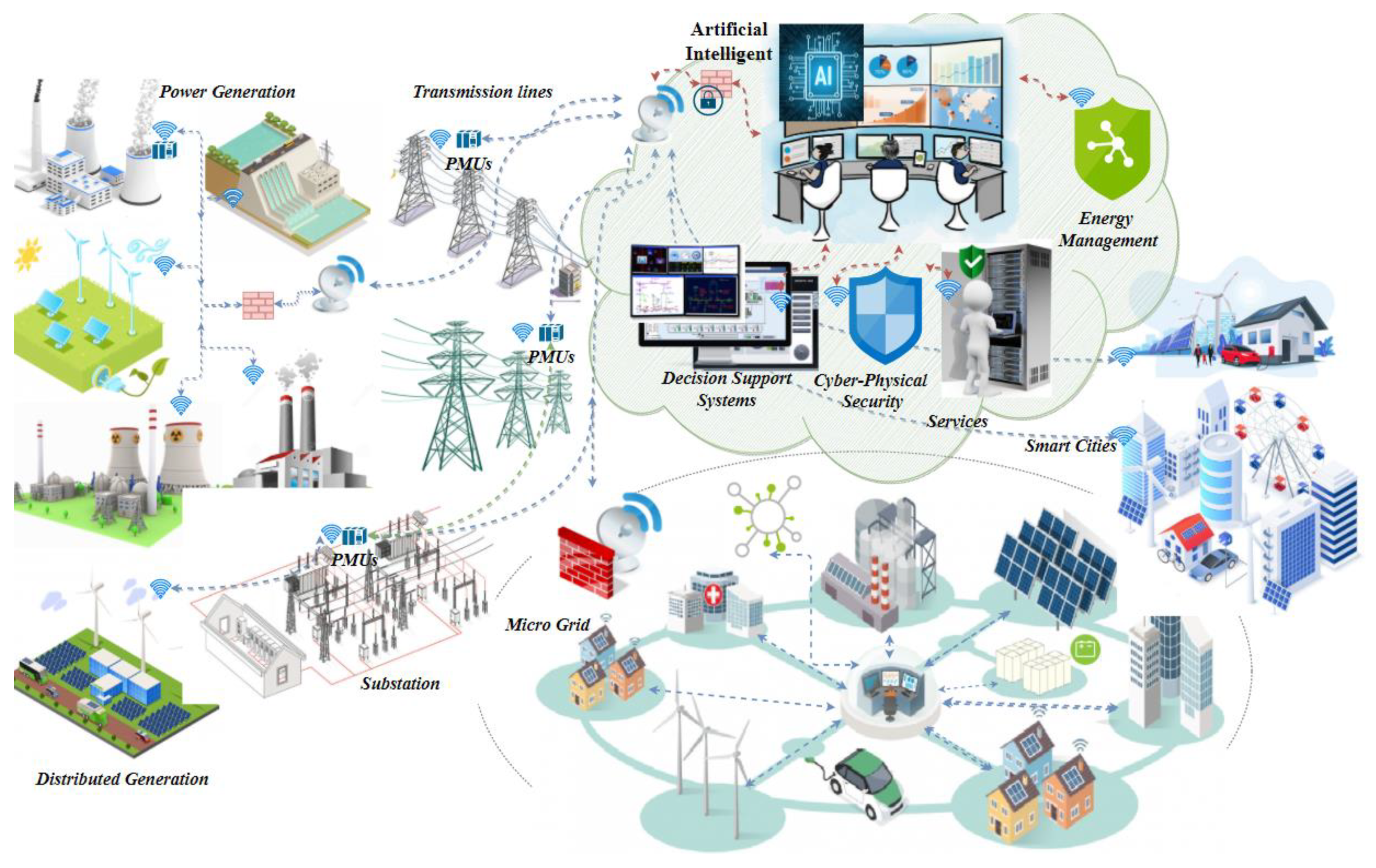
In Figure 1, a generic SG architectural view shows high integration, vast interaction, informative interoperability, and a complex power network. It merges between the different levels of consumption, generation, distribution, and other CPS entities (such as micro-grids, electric vehicles (EVs), distributed generation, smart buildings, etc.). The main domains of the SG can generate, store, and deliver electricity in two ways, which imposed the need for robust AI algorithms to improve the security, reliability, stability, and resiliency of the grid.
The increasing deployment of the intelligent embedded systems to the SG due to the dynamic power behavior of the end-users has led to integrating the Information Technology (IT) with the physical side of the grid. In order to get a much more factual picture of the voltage stability phenomena, it is crucial to consider the dynamic behavior of the system in account [22]. On the other hand, applying traditional dynamic methods may need more computational analysis and a time-consuming process for online use. Using machine learning techniques would be an attractive alternative to overcome the aforementioned problems. This is because of the ability of the machine learning techniques to learn complex non-linear relationships and their modular structures, which allows parallel processing.
Consequently, it is indispensable to identify the stability state for the smart electric grid networks using autonomous intelligent techniques to minimize implementation risks. This paper proposes a novel machine learning-based framework to uncover the stability for SGs to provide early detection of system faults before its physical implementation process, which can minimize the instability impacts and optimize risk management. In this paper, seven machine learning techniques are modeled to classify smart electric grid network stability as either stable or unstable. To achieve the maximum classification performance, we have contrasted the seven machine learning models in terms of nine performance indicators in addition to contrasting our best-proposed model with other existing models. Eventually, the comparison outcomes revealed the competency and superiority of the optimized model over the other available models. Specifically, the contribution of this paper can be listed as follows:
- Providing comprehensive identification models that employ various machine learning architectures to classify and accurately predict the VSM records in SGs.
- Evaluating the optimized performance of the identification system on a recent and significant dataset for smart grid networks stability (SGN_Stab2018), which has achieved a high identification accuracy (99.90%) with low identification overhead (4.17 μSec) for the optimizable-SVM architecture.
- Providing an in-depth explanation of our implementation in conjunction with an extensive experimental evaluation as well as comparison with state-of-the-art models.
The remaining parts of this article are systematized as follows: the examination of related research and models are presented in Section 2. In Section 3, we provide an inclusive description for the model development workflow including details about the dataset for networked SGs, the diverse evaluation metrics, and the different examined predictive models emphasizing the optimum model architecture and specifications. Section 4 presents an extensive experimental evaluation as well as a comparison with state-of-the-art models. The main inferences that could be emphasized from the results are presented in Section 5. Lastly, in Section 6, we provide a conclusion of the research work.
2. Literature Review
Many dissertations/papers have been published discussing the use of AI applications in SGs. Most of the fields cover cyber security, micro-grids, load/power consumption forecasting, defect/fault detection, demand response, stability analysis, and other areas related to the technical fields of SGs. This section discusses the recent state-of-the-art works related to the stability analysis in SGs, more specifically from two sides: (i) the approaches that have treated the stability of the SGs, and (ii) the application of ML techniques to predict the behavior of the SG.
Industries must deal with high-volume data management by analyzing and evaluating data and identifying patterns within a specified period. However, SGs are highly non-linear, operating in constantly changing operating conditions and load variation in response to a disturbance. Generally, these are considered as the driving force for voltage instability. Traditionally, stability indicators have been used to estimate the operating conditions which have to be within a short time limit and require minimum computational analysis. In addition, the characteristics have to be predictable and quickly calculable [23]. However, several drawbacks of these indices include the fact that they are extremely non-linear and discrete for variable operation conditions [23,24]. One of the developments of this aspect is to improve parameters’ measurement by using PMUs to increase the observability of the system due to their high sampling rate. In [24], a fuzzy inference system (FIS) has been discussed in order to estimate the loading margin (LM) in a real-time operation condition. Some voltage stability variables and indices are used as inputs to the FIS. To obtain better LM estimation, tuned adaptive neuro FISs and subtractive clustering are used. Dynamic stability enhancement is presented in [25,26] by measuring the grid frequency over adequate periods, linking the price directly to it, and utilizing both centralized and decentralized networks. The method was configured to eliminate or limit any non-Gaussian noise. Yet, the frequency spectrum needs to be averaged over a long time.
On the other hand, AI is considered as a more viable solution for real-time evaluation of voltage stability due to (i) Fast response by reducing the calculation time; (ii) Ability to provide knowledge about the system operation; (iii) Fewer data storage and capacity requirements as only the important measurements are used; and (iv) Ability to provide stability evaluation over a vast range of scenarios simultaneously. AI based-techniques (such as artificial neural networks (ANNs) [27], extreme learning machine (ELM) [28,29], fuzzy logic (FL) [30], and deep ensemble anomaly [31]) have drawn researchers’ attention as a solution for the evaluation of voltage stability near real time due to their ability to solve non-linear problems with desired speed and accuracy [27,28,29,30,31,32].
ANN algorithms have been widely used in both short and long-term power system voltage stability assessment due to their ability to conduct computational analysis for complex non-linear mapping. Several ANN approaches (such as backpropagation [27], Radial Basis Function (RBF) [33,34], Kohonen [35], etc.) have been reported in scientific works. ANNs need to generate many operating conditions during the training and testing processes. Therefore, power system simulations are used to establish a relationship between voltage stability indicators (such as bus and line voltage stability indices and loading margin (LM)) [28] and the measurable parameters used as input variables (such as bus voltage magnitudes and angles, real and reactive power flows and injections, branch currents, etc.) [36]. The assessment of voltage stability using ANN with reduced input sets is discussed in [37,38]. They applied a methodology to eliminate redundant measurements, which minimize the variables required to support voltage stability analysis. However, this methodology considered a large number of measurements available. To reduce the high computational processes, [39] suggested installing PMUs on a few nodes to overcome economic issues and minimize the data storage. Utilizing the PMUs measurements, both the computational and communication burdens for large power systems have been reduced. On the other hand, ANNs still exhibit some shortcomings related to the excessive training time and large sets of data required [17,18,19].
Several researchers applied ELM [28,29] to evaluate online long-term voltage stability, and different input vectors were considered (such as active and reactive power flows and injections as well as voltage magnitudes and angles). An assembled ELM is proposed in [39] to develop the performance of the power system voltage stability using VSM estimation. However, the method needs extra time for training the ELM set. The authors in [40] have presented a methodology for long-term online voltage stability monitoring in power systems that exploits the feasibility of phasor-type information, the measurements were collected using PMUs, and the power system has been divided into sub-areas to improve the supervision.
SVM or/and its regression version, support vector regression (SVR), have been used for online voltage stability based on minimizing the structural risk and improving the statistical learning. The authors in [41] have proposed a bidirectional evaluation algorithm of VSM to be used for the large penetration of photovoltaic (PV) arrays in the SG system. A deep ensemble model was developed to collect data from the AMI to be able to classify the source of variability using simultaneous point and probabilistic predictions. An evolved technique through the VSM index called Kernel Extreme Learning Machine (KELM) has been proposed by [28] for long-term voltage stability. The methodology, which is an amalgamation of both kernel-type AI and ELM, has decreased the training time and improved the performance.
Generally, stability issues rarely happen in power systems, and thus, the features associated are difficult to extract. However, the authors in [42] proposed a data mining technique for short-term online stability assessment by improving the ML imbalance training and detection. They implement a discriminative subsequence classification algorithm and a forecasting-based non-linear synthetic minority oversampling to alleviate the distortion. In [43], an active learning technique is proposed to overcome the problems associated with the existing ML applications such as prediction time, training time, and accuracy. The authors in [44] proposed Multidirectional Long Short-Term Memory (MLSTM) to predict the voltage stability of the SG network. A comparison with several DL algorithms has been evaluated. Yet, the algorithm proposed is complex and requires a high computational process.
3. Proposed Predictive Model
Typically, predictive modeling is a data-driven methodology of predicting future trends/states based on a number of historical data modeling. As such, the development of a data-driven identification/predictive model for SG stability is proposed in this research. The workflow diagram of the proposed predictive model development is illustrated in Figure 2. The process started by collecting the representative dataset to formulate the basis for the autonomous detection/identification system, passing through several preprocessing actions to produce the data records in the form that can be adequate for machine learning models, processing through various machine learning techniques, evaluating using several evaluation metrics in order to pick up the optimal ML technique (which is SVM in our case) to model and validate the proposed problem statement, and lastly using it to provide the final data predictions (identification) for the SG stability status as either stable or unstable.
3.1. Data Collection Process
In this research, the benchmark training of the SG stability (SGN_Stab2018) simulated dataset is compiled from the UCI machine learning repository [45] to validate the proposed SVM approach. This dataset was originally collected by the Karlsruhe Institute of Technology, in November 2018, by using the local stability analysis of four-buses star system implementing a decentralized SG controller concept. Each item stands for the predictive attributes on a scale of [0, 10]. The dataset comprises 10,000 samples (divided into 3620 stable samples and 6380 unstable samples) with 13 input features and one output feature for binary class labeling (to identify the system status for SG as either stable or unstable). In order to predict the stability condition of a given system, this research exploits VSM as the output feature to be predicted. A VSM value closer to 1 indicates that the system is reaching its voltage collapse point. The input features contain specific parameters that need to be specified and generated from the following functions:
- Reaction time () value for energy producer () and three consumers (, , and ) where:
- Nominal power () of consumer or producer () where:
- The regularization parameter () related to price elasticity () where:
- The maximum characteristic value of the root equation (
The system’s output is the maximum real part of the characteristic differential equation root (stab). The acquired data are cleaned from empty and misleading samples. Since the data have different scales, data normalization is essential to unify the range of data. The best solution for a large dataset is to eliminate the total rows containing missing values [46]. The final data are divided into three folds, 70% of the data is devoted to training and validation. The remaining 30% is used for testing purposes.
3.2. Data Engineering Actions
The measurements of the SG systems are very redundant, and the number of variables is considerably high. Thus, restricting the input space to a small subset of the available input variables has explicit economic benefits in terms of computational requirements, cost, and data storage of future data collection. Furthermore, lowering the number of input variables derives more understanding of the model; i.e., the optimum dataset variables are considered to be the set that has a smaller number of input variables with no uninformative variables, and a minimum degree of redundancy is used to characterize the output behavior of the system. Typically, data engineering or data preprocessing is a key module in every machine/deep learning system, similar to any machine learning-based system. In this module, data records pass through a number of preprocessing actions to prepare the dataset samples for the learning process [46]. In this research, our target dataset has undergone the following processes:
- Transformation process: converting the data from comma-separated values into a double matrix of vectored dataset instances each with 14 columns (14 × 10,000).
- Class labeling process: representing the categorical class feature into a binary label ().
- Dataset randomizing or shuffling process: re-allocating the instances into the dataset to help the training process to converge fast and preclude any bias throughout the training process.
- Splitting up: dividing the dataset into two datasets with random indices where 70% of the data records are used for the training process and the remaining 30% of the data records are used for the testing process.
To confirm a confident validation (testing) process, we have conducted five-fold cross-validation [47] that incorporated five dissimilar experiments for each machine learning model with different subsets for training and validation processes designated for each experiment after data shuffling.
3.3. Applied Machine Learning Techniques
In this stage, we applied the preprocessed data into different machine learning techniques in order to investigate their performance metrics to contrast them accordingly. In this research, our preprocessed dataset has been applied using the following machine learning techniques:
- Support Vector Machines (SVM): Supervised learning model and usually used as a linear binary classifier [48] to address classification and regression problems. SVM can be used to solve linear and non-linear problems for various real-life applications. The basic idea of SVM classification is to create a line or a hyperplane that can separate the data into two classes, which will be discussed thoroughly in the next section.
As a result, our SVM-based model has been configured with Linear SVM as a kernel function, in which the kernel scale is set to 0.001–1000 and the box constraint level is 9946 (should be constrained between 0.001 and 1000, and the larger the better) with Bayesian optimizer with a standardized dataset. Finally, the total misclassification cost is 59 samples.
- Logistic Regression Classifier (LRC): Supervised learning model and usually used as a binary classifier [49] by building an equation. LRC aims to discover the most suitable set of model parameters where every input feature () of the LRC model is multiplied by a weight (), and thereafter, all values () are summed together with a bias value (). After that, accumulated sums are passed through the sigmoid function ()) to generate the binary class outputs. In this paper, we have employed logit function metric as a cost function in the logistic regression classifier to evaluate classification probability. A typical logistic probability will never go below 0 and above 1, and the logistic cost function can be calculated for each sample (x) from the total number of samples (m) with probability (p) as:
As a result, our logistic regression-based model has been configured with logit function as a loss/cost criterion, sigmoid function as an output classification, and the total number of misclassifications is 101 samples with all features used in the model.
- Decision Tree Classifier (DTC): Supervised learning mechanism that can be used for predictive models (classification/regression) having a tree-like structure [50]. The decision tree deals with the features of the dataset and builds the learning model by splitting the dataset based on its features of datasets, where the best feature of the dataset is placed at the root node. This procedure is continually performed until all the features of the dataset are split, reaching the leaf node at each branch. Thereafter, a decision tree uses estimates and probabilities to calculate likely outcomes. In this paper, since we are dealing with a binary classification problem (target variable “Stable” or “Unstable”), we have employed the Gini index metric as a cost function in the decision tree to evaluate splits in the dataset. The Gini index for each node of the tree (i) of all nodes (C) probability () is given as:
As a result, our decision tree-based model has been configured with the Gini index as the split criterion, and the maximum number of splits is 100 with no surrogate decision splits. Finally, the total misclassification cost is 82 samples.
- Naïve Bayes Classifier (NBC): Supervised learning mechanism used for constructing classifiers based on Bayes theorem [51]. Naïve Bayes is a conditional probability approach used to predict the likelihood that an event will occur, given evidence defined in the data feature. Naïve Bayes is used for probabilistic classification and regression purposes. In this paper, we employed Gaussian naïve Bayes for a numeric predictors algorithm to provide two-class classification. Given a data instance with an unknown class label, is the hypothesis that belongs to a specific class ; then, the conditional probability of hypothesis given observation is denoted:
As a result, our naïve Bayes-based model has been configured with multivariate multinomial (mvmn) distribution as a binary categorical predictor, and the total number of misclassifications is 211 with PCA (principal component analysis) configured over the features.
- Linear Discriminant Classifier (LDC): A dimensionality reduction method that is generally employed to address supervised classification tasks [52] by separating the data labels into two or more classes. The basic idea of LDC is to project the features in higher dimension space into a lower dimension space. For example, we have two classes, and we need to separate them efficiently. LDC starts the classification by using only a single feature, and then, we will keep on increasing the number of features for proper classification. In this paper, since we are dealing with a binary classification problem (target variable “Stable” or “Unstable”), we have employed Fisher’s Linear Discriminant (FLD) with two-dimensional input vector projection to classify between two classes of the target feature. Given that N1 and N2 denote the number of samples in classes C1 (Stable) and C2 (Unstable), respectively, then, we find the projection ) using FLD, which learns a weight vector W, where m1 and m2 are the mean vectors for the two classes, and S1 and S2 are the variance vectors for the two classes, using the following criterion:
As a result, our linear discriminant-based model has been configured with a full covariance structure as a binary categorical predictor, and the total number of misclassifications is 312 with PCA (principal component analysis) configured over the features.
- k-Nearest Neighbor (kNN): [53] A supervised machine learning classifier that memorizes the labeled observations within the training dataset to predict classifications for new unlabeled observations. kNN is among the simplest and most easy-to-implement classifications, and it makes its predictions based on similarity. Similarity comparisons can be based on any quantitative attribute such as weather, distance, age, income, and weight (the simplest and most common comparative attribute is distance). In this paper, we have employed k-nearest neighbor with k set to one neighbor and the Euclidian function as a distance metric function to evaluate the degree of neighborhood for every sample in the dataset. The Gini index for each node of the tree (i) of all nodes (C) probability () is given as:
As a result, our kNN-based model has been configured with the Euclidian index as the distance criterion with the distance weight set to true, and the total number of misclassifications is 1008 samples with a standardized dataset.
- Ensemble Boosted Classifier (EBC): Supervised learning method that employs multiple learners (weak learners/models) to resolve the identified classification problem and then aggregate their outcomes to produce the final output [54]. Aggregation can be done using a boosting mechanism that creates a strong classifier by combining the final result from a number of sequential homogeneous weak learners using a deterministic aggregation approach. In this paper, we have employed the RUSBoost mechanism as an ensemble method and the decision tree as a classification learner to evaluate splits in the dataset.
As a result, our ensemble-based RUSBoost-based model has been configured with the Gini index as the split criterion; the maximum number of splits is 20, using 30 learners with a learning rate of 0.1 and no surrogate decision splits. Finally, the total misclassification cost is 2896 samples.
3.4. Evaluation Metrics
To pick up the best predictive model that can be used to identify the stability state of the electrical smart grid defined by the target dataset, we need to evaluate the proficiency of the machine learning models employed in this research. One should first investigate the binary confusion matrix [55] to provide the values for true positive (), true negative (), false-positive (), and false-negative (). In addition, we have used the following key performance indicators [56]:
- Model Accuracy () measures the ability of the system to provide correct sample classification with respect to the whole number of samples and is given as:
- Positive Predictive Value () measures the ability of the system to provide correct sample classification with respect to the positive number of samples and is given as:
- True Positive Rate () measures the ability of the system to provide correct sample classification with respect to the number of samples that should be retrieved and is given as:
- Harmonic Mean Score () is a weighted score for the relation between Positive Predictive Value () and True Positive Rate () and is given as:
- False Alarm Rate () measures the proportion that the system provides incorrect sample classification with respect to the whole number of samples and is given as:
- False Discovery Rate () measures the proportion that the system provides incorrect sample classification with respect to the positive number of samples and is given as:
- False Negative Rate () measures the proportion that the system provides incorrect sample classification with respect to the number of samples that should be retrieved and is given as:
- Area Under Curve () measures the ability of the system to rank a randomly selected positive sample higher than a randomly selected negative sample and is given as:
- Identification Speed () measures the number of samples that the system can process within the unit and is given as:
- Identification Delay (IDD) measures the time required by the system to provide a single sample prediction (in ) and is given as:
3.5. Predictive Model-Based SVM
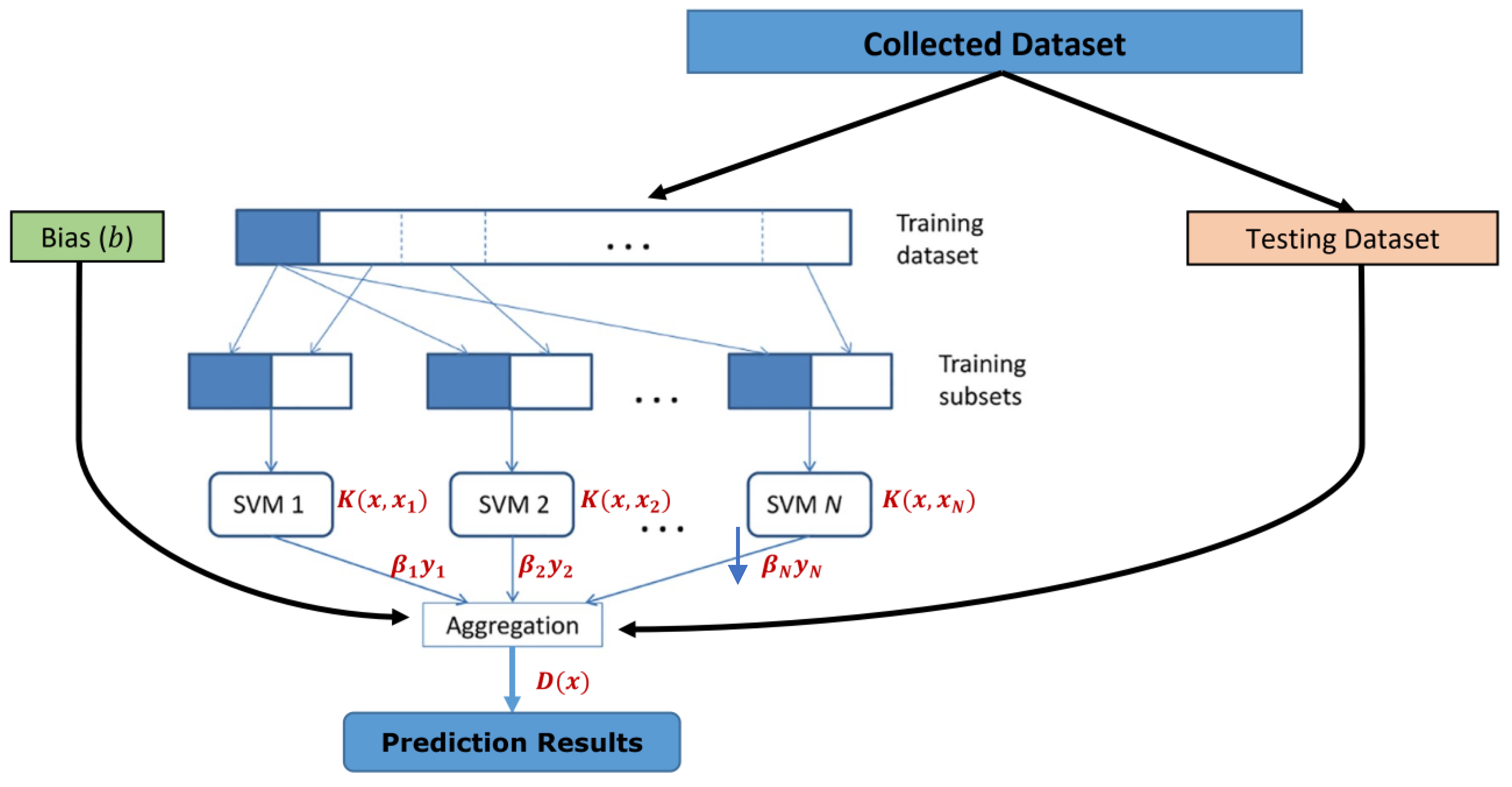
As we will see in the next section, after evaluating all the aforementioned ML models using the prescribed evaluation metrics, we end up concluding that the SVM model is the optimal ML technique to model and validate the proposed problem statement of identifying the SG stability status as either stable or unstable. SVM is a supervised machine learning approach that is employed for the application of prediction and classification [57]. By applying the training records, each is categorized to a certain category. SVM is a non-parametric technique, since it comprises a number of weighted vectors, nominated from the training dataset, where the number of support vectors is less than or equal to the number of training samples. For example, in ML applications for natural language processing (NLP), it is not unheard of to have SVMs with tens of thousands of vectors each comprising hundreds of thousands of data features [58]. Figure 3 illustrates the architecture of the SVM technique employed in our predictive model.
According to Figure 3, in the beginning, the bootstrapping technique [59] is used to create a number of SVMs (1, 2, … N) which are assigned dynamically by the automatic classification learner tool. These training subsets are created by randomly resampling with replacement from the original training dataset repeatedly. Every SVM is trained distinctly with the training subsets generated from the original training dataset, and once the training process is completed, the trained SVMs are aggregated using a suitable combination approach such as the following binary sign ensemble aggregation function that is used in our binary classification system:
: are the linear outputs from every SVM (1, 2, …., N).
: is the classifier bias, in default, it is set to .
A kernel function is applied by each SVM to fit the non-linear models into a higher dimensional space (via “kernels”) before finding the optimal hyperplane to separate the classes. Typically, the formula of the Radial Basis Function (RBF) kernel [60] is commonly used, and it is also used in this paper and defined as follows:
4. System Evaluation and Results
In this section, we provide extensive simulation results that have been obtained from the evaluation of the seven above-mentioned machine learning models using the prescribed evaluation metrics. Table 1 contrasts the performance of the examined supervised machine learning models (SVM, DTC, LLRC, NBC, LDC, kNN, and EBC) in terms of ACC, FAR, PPV, FDR, TPR, FNR, HMS, and IDS metrics. To gain more insights into these results of predictive models, we are visualizing the comparison of predictive models in terms of four quality indication metrics (ACC, PPV, TPR, and HMS) in Figure 4A and the comparison of predictive models in terms of three error analysis metrics (FAR, FDR, and FNR) in Figure 4B, respectively.
Figure 5 contrasts the seven experimented machine learning techniques in terms of four quality indication metrics and three error analysis metrics for the proposed stability identification model of the smart electric grid network. According to the figure, the best performance metrics are registered for the SVM model with the highest quality indicators of 99.93%, 99.89%, 99.92%, and 98.62% for ACC, PPV, TPR, and HMS, respectively, and lowest error indicators of 0.07%, 0.11%, and 0.08% for FAR, TDR, and FNR, respectively. Conversely, the lowest performance metrics are registered for EBC model with lowest quality indicators of 71.04%, 68.80%, 60.00%, and 63.75% for ACC, PPV, TPR, and HMS respectively, and highest error indicators of 28.96%, 31.20%, and 40.00% for FAR, TDR, and FNR, respectively. In addition, other noticeable and comparable classifiers/alternatives are the DTC and LRC, which recorded very high accuracy measures with 99.18% and 98.99% for DTC and LRC. However, DTC performed slower with higher perdition delay than LRC (i.e., 11.90 μSec vs. 7.14 μSec for DTC and LRC, respectively). Moreover, another important feature that distinguishes our optimized SVM model is the prediction time/speed, which is identified as the fastest classifier scoring the minimum prediction delay with only 4.17 μSec for the sample prediction. In contrast, the slowest classifier was the kNN model scoring the maximum prediction delay with 83.33 μSec for the sample prediction.
As we demonstrated from the last table, figures, and discussion, the optimizable SVM classifier has been picked up as the best classifier to provide the final data predictions (identification) for the smart electric grid network stability status as either stable or unstable. Therefore, the next figures, discussion, and analysis will focus on the SVM model. Hence, Figure 5 illustrates the performance evaluation for the developed optimizable SVM classifier using a minimum classification error plot after 30 iterations of the optimization process. The plot tracks the trajectories for the estimated minimum classification error and the observed minimum classification error. As can be seen, both error trajectories (estimated and observed) follow a decreasing tendency with the increasing iterations before they are both saturated after almost 17 iterations of the optimization process where the best point hyperparameters have a minimum classification error . Such very low values for the minimum classification error allowed the system to record the highest prediction accuracy for the target dataset.
Moreover, Figure 6 demonstrates the comprehensive diagram for the confusion matrix analysis. Specifically, the figure shows (from top-left toward bottom-right): the confusion matrix parameters obtained for our SVM model with (TP = 3617, FN = 3, FP = 4, and TN = 6376), TPR vs. FNR analysis for each individual class (both classes scored TPR = 99.9% and TNR = 0.1%), PPV vs. FDR analysis for each individual class (both classes scored PPV = 99.9% and TDR = 0.1%), and the general two-class confusion matrix parameters employed to measure the quality and error indicators (mentioned earlier). According to the figure, the confusion matrix outcomes clearly indicate the high quality and optimality of the voltage stability prediction process of our optimizable SVM model, and thus, this is the main reason to record the best performance evaluation metrics.
Furthermore, Figure 7 visualizes the plots for area under curve (AUC) for each class (stable and unstable). AUC curves investigate the association between true and false-positive rates (TPR vs. FPR) at different prediction thresholds [61]. AUC provides a mean of the system’s ability to rank a randomly selected positive sample higher than a randomly selected negative sample as an area of percentages from (0,0) to (1,1) for each axis. For that reason and according to the AUC plots in Figure 7, it can be concluded that both classes exhibit perfect ranking measurements, recording AUC values of 100%.
5. Discussion and Evaluation
The stability of the SG is decidedly influenced by objective conditions such as transmission line aging, power generation limitations, dynamic behavior and intermittent loads, volatile behavior of RES, etc. An efficient identification system is proposed to predict the smart grid stability margin based on pre-established computational features and is implemented, analyzed, and assessed in this paper. The following inferences can be emphasized from the results:
- Voltage instability phenomenon is considered the main threat to stability, security, and reliability in modern power systems. Due to the load changes and sudden contingencies occurrence, off-line voltage stability monitoring can no longer ensure a secure operation of the power system. Hence, fast and efficient methods to assess power system voltage stability are of great importance to experts and industries in order to avoid the risk of large blackouts.
- Focusing on point prediction and interval forecasting is extremely important to weaken the uncertainty and support the grid stability-based SG paradigm. So, this paper developed an efficient computing framework to solve the Smart Grid Stability Prediction. An electrical grid stability simulated dataset was considered for the validation of the proposed approach.
- Even though this is the first research work to address the stability status prediction for the electric smart grid network using conventional machine learning techniques (to the best of our knowledge), we still can compare it with other state-of-art techniques that employ the same dataset using deep learning techniques [62]. Therefore, Table 2 contrasts all applicable evaluation metrics with the results we obtained for our optimizable SVM model. Based on the information provided in the table, we can clearly see that the proposed predictive model is comparable and superior in several evaluation metrics even though it is less complex and has a lower prediction overhead than the other deep learning models provided in the table. In addition, we have provided an overall metric in the last column (overall score) that averages the values of metrics associated with the same model to come up with a single score to represent the overall quality for the predictive model. Although all models in the table have recorded a high overall score, the proposed predictive model has recorded the highest overall score (i.e., 99.93%) among all models in the table where the model achieved a 1.02–3.67% increase in the overall metric.
- For applications with a higher dimensional dataset, future work could further improve the proposed framework’s performance by combining the proposed technique with big data frameworks to improve the prediction model’s operational efficiency for longer prediction horizons. Furthermore, this method can be implemented for other applications to smart grids, such as power and load forecasting, to increase energy efficiency.
6. Conclusions and Remarks
A novel efficient identification system to predict the stability of smart grid networks based on pre-established computational features is implemented, analyzed, and assessed in this paper. The proposed system tends to provide precocious warnings/alarms of smart grid system faults that can minimalize/avoid the instability impacts at the physical implementation phases for the smart grid system. The developed model employs seven machine learning techniques to classify smart electric grid network stability into either stable or unstable, namely, Optimizable-Support Vector Machine (SVM), Decision Trees Classifier (DTC), Logistic Regression Classifier (LRC), Naïve Bayes Classifier (NBC), Linear Discriminant Classifier (LDC), k-Nearest Neighbor (kNN), and Ensemble Boosted Classifier (EBC). The developed ML models have been assessed using a contemporary and inclusive smart grid network stability dataset (SGN_Stab2018) in terms of several performance indicators including binary confusion matrix (BCM), identification accuracy (ACC), positive predictive value (PPV), true positive rate (TPR), harmonic mean score (HMS), false alarm rate (FAR), false discovery rate (FDR), false-negative rate (FNR), area under curve (AUC), identification speed (IDS), and identification delay (IDD). Accordingly, the seven machine learning models have been contracted in terms of identified performance indicators to exploit the maximum system performance. Ultimately, the comparison outcomes have revealed the competency and superiority of the optimized model over the other available models. Our best-obtained performance outcomes have surpassed the performance outcomes for the existing smart grid networks’ stability predictive models.
Author Contributions
Conceptualization, Q.A.A.-H.; methodology, Q.A.A.-H.; soft-ware, Q.A.A.-H.; validation, A.A.S. and M.F.A.; formal analysis, Q.A.A.-H. and A.A.S.; investigation, Q.A.A.-H.; resources, Q.A.A.-H. and A.A.S.; data curation, Q.A.A.-H., writing—original draft preparation, Q.A.A.-H. and A.A.S.; writing—review and editing, Q.A.A.-H., A.A.S. and M.F.A..; visualization, Q.A.A.-H., A.A.S. and M.F.A.; supervision, Q.A.A.-H.; project administration, Q.A.A.-H.; funding acquisition, M.F.A. All authors have read and agreed to the published version of the manuscript.
Funding
This research received no external funding.
Data Availability Statement
Dataset employed by this research can be retrieved from UCI Machine Learning Repository, Electrical Grid Stability Dataset. https://archive.ics.uci.edu/ml/datasets, (accessed on 18 October 2021).
Acknowledgments
The authors value the distance collaboration between Princess Sumaya University for Technology/Jordan, University of Idaho/USA, and University of Tabuk/Saudi Arabia. Also, the authors gratefully acknowledge the Deanship of Scientific Research at the University of Tabuk, Saudi Arabia, for their financial support of the publication fees for this paper.
Conflicts of Interest
The authors declare no conflict of interest.
References
- Wang, T. Net Consumption of Electricity Worldwide from 1980 to 2018; Statista: Hamburg, Germany, 2021; pp. 4514–4525. Available online: http://www.eia.gov/beta/international/ (accessed on 15 August 2021).
- NaturalGas.org. Natural Gas and the Environment. 2010. Available online: http://www.naturalgas.org/environment/naturalgas.asp (accessed on 15 September 2021).
- Ullah, Z.; Al-Turjman, F.; Mostarda, L.; Gagliardi, R. Applications of Artificial Intelligence and Machine learning in smart cities. Comput. Commun. 2020, 154, 313–323. [Google Scholar] [CrossRef]
- Khan, S.; Paul, D.; Momtahan, P.; Aloqaily, M. Artificial intelligence framework for smart city microgrids: State of the art, challenges, and opportunities. In Proceedings of the 2018 Third International Conference on Fog and Mobile Edge Computing (FMEC), Barcelona, Spain, 23–26 April 2018; pp. 283–288. [Google Scholar]
- Bose, B.K. Artificial intelligence techniques in smart grid and renewable energy systems: Some example applications. Proc. IEEE 2017, 105, 2262–2273. [Google Scholar] [CrossRef]
- Bassamzadeh, N.; Ghanem, R. Multiscale stochastic prediction of electricity demand in smart grids using Bayesian networks. Appl. Energy 2017, 193, 369–380. [Google Scholar] [CrossRef]
- Smadi, A.; Ajao, B.; Johnson, B.; Lei, H.; Chakhchoukh, Y.; Abu Al-Haija, Q. A Comprehensive Survey on Cyber-Physical Smart Grid Testbed Architectures: Requirements and Challenges. Electronics 2021, 10, 1043. [Google Scholar] [CrossRef]
- Siano, P. Demand response and smart grids-a survey. Renew. Sustain. Energy Rev. 2014, 30, 461–478. [Google Scholar] [CrossRef]
- Lingaraju, K.; Gui, J.; Johnson, B.K.; Chakhchoukh, Y. Simulation of the Effect of False Data Injection Attacks on SCADA using PSCAD/EMTDC. In Proceedings of the 2020 52nd North American Power Symposium (NAPS), Tempe, AZ, USA, 11–13 October 2020; pp. 1–5. [Google Scholar]
- Chen, Y.T. Modeling information security threats for smart grid applications by using software engineering and risk management. In Proceedings of the 2018 IEEE International Conference on Smart Energy Grid Engineering (SEGE), Oshawa, ON, Canada, 12–15 August 2018; pp. 128–132. [Google Scholar]
- Cai, X.; Wang, Q.; Tang, Y.; Zhu, L. Review of Cyber-attacks and Defense Research on Cyber Physical Power System. In Proceedings of the 2019 IEEE Sustainable Power and Energy Conference (iSPEC), Beijing, China, 20–24 November 2019; pp. 487–492. [Google Scholar] [CrossRef]
- Radoglou-Grammatikis, P.I.; Sarigiannidis, P.G. Securing the Smart Grid: A Comprehensive Compilation of Intrusion Detection and Prevention Systems. IEEE Access 2019, 7, 46595–46620. [Google Scholar] [CrossRef]
- Reports of Energy. Grid 2030: A National Vision for Electricity’s Second 100 Years; Tech. Report; Department of Energy: Washington, WA, USA, 2003.
- Lanzrath, M.; Suhrke, M.; Hirsch, H. HPEM-Based Risk Assessment of Substations Enabled for the Smart Grid. IEEE Trans. Electromagn. Compat. 2019, 62, 173–185. [Google Scholar] [CrossRef]
- Ramchurn, S.D.; Vytelingum, P.; Rogers, A.; Jennings, N.R. Putting the ‘smarts’ into the smart grid: A grand challenge for artificial intelligence. Commun. ACM 2012, 55, 86–97. [Google Scholar] [CrossRef] [Green Version]
- Industrial Controllers Still Vulnerable to Stuxnet-Style Attacks. Available online: https://www.securityweek.com/industrial-controllers-still-vulnerable-stuxnet-style-attacks (accessed on 11 September 2021).
- Hackers Breached Colonial Pipeline Using Compromised Password. Available online: https://www.bloomberg.com/news/articles/2021-06-04/hackers-breached-colonial-pipeline-using-compromised-password (accessed on 11 September 2021).
- Cyber Autopsy Series: Ukrainian Power Grid Attack Makes History. Available online: https://www.globalsign.com/en/blog/cyber-autopsy-series-ukranian-power-grid-attack-makes-history (accessed on 11 September 2021).
- Wadhawan, Y.; Almajali, A.; Neuman, C. A Comprehensive Analysis of Smart Grid Systems against Cyber-Physical Attacks. Electronics 2018, 7, 249. [Google Scholar] [CrossRef] [Green Version]
- Heide, D.; von Bremen, L.; Greiner, M.; Hoffmann, C.; Speckmann, M.; Bofinger, S. Seasonal optimal mix of wind and solar power in a future, highly renewable Europe. Renew. Energy 2010, 35, 2483–2489. [Google Scholar] [CrossRef]
- Lind, P.G.; Wächter, M.; Peinke, J. Reconstructing the intermittent dynamics of the torque in wind turbines. J. Physics: Conf. Ser. 2014, 524, 012179. [Google Scholar] [CrossRef]
- Ratra, S.; Tiwari, R.; Niazi, K.R. Voltage stability assessment in power systems using line voltage stability index. Comput. Electr. Eng. 2018, 70, 199–211. [Google Scholar] [CrossRef]
- Gomez-Exposito, A.; Conejo, A.J.; Canizares, C. Electric Energy Systems: Analysis and Operation; CRC Press: Boca Raton, FL, USA, 2018. [Google Scholar]
- Torres, S.P.; Peralta, W.H.; Castro, C.A. Power System Loading Margin Estimation Using a Neuro-Fuzzy Approach. IEEE Trans. Power Syst. 2007, 22, 1955–1964. [Google Scholar] [CrossRef]
- Schäfer, B.; Grabow, C.; Auer, S.; Kurths, J.; Witthaut, D.; Timme, M. Taming instabilities in power grid networks by decentralized control. Eur. Phys. J. Spec. Top. 2016, 225, 569–582. [Google Scholar] [CrossRef]
- Schäfer, B.; Matthiae, M.; Timme, M.; Witthaut, D. Decentral smart grid control. New J. Phys. 2015, 17, 15002. [Google Scholar] [CrossRef]
- AlOmari, A.A.; Smadi, A.A.; Johnson, B.K.; Feilat, E.A. Combined Approach of LST-ANN for Discrimination between Transformer Inrush Current and Internal Fault. In Proceedings of the 2020 52nd North American Power Symposium (NAPS), Tempe, AZ, USA, 11–13 October 2020; pp. 1–6. [Google Scholar]
- Villa-Acevedo, W.M.; López-Lezama, J.M.; Colomé, D.G. Voltage Stability Margin Index Estimation Using a Hybrid Kernel Extreme Learning Machine Approach. Energies 2020, 13, 857. [Google Scholar] [CrossRef] [Green Version]
- Duraipandy, P.; Devaraj, D. Development of extreme learning machine for online voltage stability assessment incorporating wind energy conversion system. In Proceedings of the 2017 IEEE International Conference on Intelligent Techniques in Control, Optimization and Signal Processing (INCOS), Tamil Nadu, India, 23–25 March 2017; pp. 1–7. [Google Scholar]
- Edris, A.; Alajlan, A.; Sheldon, F.; Soule, T.; Heckendorn, R. An Alert System: Using Fuzzy Logic for Controlling Crowd Movement by Detecting Critical Density Spots. In Proceedings of the 2020 International Conference on Computational Science and Computational Intelligence (CSCI), Las Vegas, NV, USA, 16–18 December 2020; pp. 633–636. [Google Scholar]
- Albulayhi, K.; Sheldon, F.T. An Adaptive Deep-Ensemble Anomaly-Based Intrusion Detection System for the Internet of Things. In Proceedings of the 2021 IEEE World AI IoT Congress (AIIoT), Seattle, WA, USA, 10–13 May 2021; pp. 187–196. [Google Scholar]
- Albulayhi, K.; Smadi, A.A.; Sheldon, F.T.; Abercrombie, R.K. IoT Intrusion Detection Taxonomy, Reference Architecture, and Analyses. Sensors 2021, 21, 6432. [Google Scholar] [CrossRef]
- Gonzalez, J.W.; Isaac, I.A.; Lopez, G.J.; Cardona, H.A.; Salazar, G.J.; Rincon, J.M. Radial basis function for fast voltage stability assessment using Phasor Measurement Units. Heliyon 2019, 5, e02704. [Google Scholar] [CrossRef]
- Hashemi, S.; Aghamohammadi, M.R. Wavelet based feature extraction of voltage profile for online voltage stability assessment using RBF neural network. Int. J. Electr. Power Energy Syst. 2013, 49, 86–94. [Google Scholar] [CrossRef]
- De, A.; Chakraborty, K.; Chakrabarti, A. Classification of power system voltage stability conditions using Kohonen’s self-organizing feature map and learning vector quantization. Eur. Trans. Electr. Power 2012, 22, 412–420. [Google Scholar] [CrossRef]
- Nakawiro, W.; Erlich, I. Online voltage stability monitoring using Artificial Neural Network. In Proceedings of the Third International Conference on Electric Utility Deregulation and Restructuring and Power, Nanjing, China, 6–9 April 2008. [Google Scholar]
- Bahmanyar, A.; Karami, A. Power system voltage stability monitoring using artificial neural networks with a reduced set of inputs. Int. J. Electr. Power Energy Syst. 2014, 58, 246–256. [Google Scholar] [CrossRef]
- Ashraf, S.M.; Gupta, A.; Choudhary, D.K.; Chakrabarti, S. Voltage stability monitoring of power systems using reduced network and artificial neural network. Int. J. Electr. Power Energy Syst. 2017, 87, 43–51. [Google Scholar] [CrossRef]
- Zhang, R.; Xu, Y.; Dong, Z.Y.; Zhang, P.; Wong, K.P. Voltage stability margin prediction by ensemble based extreme learning machine. In Proceedings of the 2013 IEEE Power Energy Society General Meeting, Vancouver, BC, USA, 21–25 July 2013; pp. 1–5. [Google Scholar]
- Villa-Acevedo, W.M.; López-Lezama, J.M.; Colomé, D.G.; Cepeda, J. Long-term voltage stability monitoring of power system areas using a kernel extreme learning machine approach. Alex. Eng. J. 2021. [Google Scholar] [CrossRef]
- Alazab, M.; Khan, S.; Krishnan, S.S.R.; Pham, Q.-V.; Reddy, M.P.K.; Gadekallu, T.R. A Multidirectional LSTM Model for Predicting the Stability of a Smart Grid. IEEE Access 2020, 8, 85454–85463. [Google Scholar] [CrossRef]
- Wu, Q.; Han, B.; Shahidehpour, M.; Li, G.-J.; Wang, K.; Luo, L.; Jiang, X. Deep Ensemble With Proliferation of PV Energy for Bidirectional Evaluation of Voltage Stability Margin. IEEE Trans. Sustain. Energy 2019, 11, 771–784. [Google Scholar] [CrossRef]
- Malbasa, V.; Zheng, C.; Chen, P.-C.; Popovic, T.; Kezunovic, M. Voltage Stability Prediction Using Active Machine Learning. IEEE Trans. Smart Grid 2017, 8, 3117–3124. [Google Scholar] [CrossRef]
- Zhu, L.; Lu, C.; Dong, Z.Y.; Hong, C. Imbalance Learning Machine-Based Power System Short-Term Voltage Stability Assessment. IEEE Trans. Ind. Inform. 2017, 13, 2533–2543. [Google Scholar] [CrossRef]
- Arzamasov, V.; Bohm, K.; Jochem, P. Towards concise models of grid stability. In Proceedings of the IEEE International Conference on Communications, Control, and Computing Technologies for Smart Grids (SmartGridComm), Aalborg, Denmark, 29–31 October 2018; pp. 1–6. [Google Scholar]
- Abu Al-Haija, Q.; Zein-Sabatto, S. An Efficient Deep-Learning-Based Detection and Classification System for Cyber-Attacks in IoT Communication Networks. Electronics 2020, 9, 2152. [Google Scholar] [CrossRef]
- Gupta, P. Cross-Validation in Machine Learning. Medium towards Data Sci. 2017. Available online: https://towardsdatascience.com/cross-validation-in-machine-learning-72924a69872f (accessed on 13 February 2020).
- Li, H.; Chung, F.-L.; Wang, S. A SVM based classification method for homogeneous data. Appl. Soft Comput. 2015, 36, 228–235. [Google Scholar] [CrossRef]
- Kirin, R.V. A Theoretical Analysis of Logistic Regression and Bayesian Classifiers. arxiv 2021, arXiv:2108.03715. [Google Scholar]
- Abu Al-Haija, Q.; Alsulami, A.A. High Performance Classification Model to Identify Ransomware Payments for Heterogeneous Bitcoin Networks. Electronics 2021, 10, 2113. [Google Scholar] [CrossRef]
- Berrar, D. Bayes’ theorem and naive Bayes classifier. In Encyclopedia of Bioinformatics and Computational Biology: ABC of Bioinformatics; Elsevier Science Publisher: Amsterdam, The Netherlands, 2018; pp. 403–412. [Google Scholar]
- Tharwat, A. Linear vs. quadratic discriminant analysis classifier: A tutorial. Int. J. Appl. Pattern Recognit. 2016, 3, 145–180. [Google Scholar] [CrossRef]
- Gazalba, I.; Reza, N.G.I. Comparative analysis of k-nearest neighbor and modified k-nearest neighbor algorithm for data classification. In Proceedings of the 2017 2nd International Conferences on Information Technology, Information Systems and Electrical Engineering (ICITISEE), Yogyakarta, Indonesia, 1–2 November 2017; pp. 294–298. [Google Scholar]
- Zhou, Z. Ensemble Methods: Foundations and Algorithms; Chapman and Hall/CRC: Boca Raton, FL, USA, 2019. [Google Scholar]
- Narkhede, S. Understanding Confusion Matrix. Medium: Towards Data Science. 2018. Available online: https://towardsdatascience.com/understanding-confusion-matrix-a9ad42dcfd62 (accessed on 12 January 2020).
- Al-Haija, Q.A.; Smadi, M.; Al-Bataineh, O.M. Identifying Phasic dopamine releases using DarkNet-19 Convolutional Neural Network. In Proceedings of the 2021 IEEE International IOT, Electronics and Mechatronics Conference (IEMTRONICS), Toronto, ON, Canada, 21–24 April 2021; pp. 1–5. [Google Scholar] [CrossRef]
- Awad, M.; Rahul, K. Support vector machines for classification. In Efficient Learning Machines; Apress: Berkeley, CA, USA, 2015; pp. 39–66. [Google Scholar]
- Ghose, A. Support Vector Machine (SVM) Tutorial: Learning SVMs from Examples. Medium. 2017. Available online: https://blog.statsbot.co/support-vector-machines-tutorial-c1618e635e93 (accessed on 15 June 2021).
- Rawat, S. Bootstrapping Method: Types, Working and Applications. Machine Learning: Statistics, by Bootstrapping Method: Types, Working and Applications. 2021. Available online: https://analyticssteps.com/blogs/bootstrapping-method-types-working-and-applications (accessed on 15 June 2021).
- Chandradevan, R. Radial Basis Functions Neural Networks—All we need to know. Medium: Towards Data Science. 2017. Available online: https://towardsdatascience.com/radial-basis-functions-neural-networks-all-we-need-to-know-9a88cc053448 (accessed on 15 March 2021).
- Badawi, A.A.; Al-Haija, Q.A. Detection of Anti-Money Laundry in Bitcoin Transactions. In Proceedings of the 4th Smart Cities Symposium (SCS), Zallaq, Bahrain, 21–23 November 2021. [Google Scholar]
- Massaoudi, M.; Abu-Rub, H.; Refaat, S.S.; Chihi, I.; Oueslati, F.S. Accurate Smart-Grid Stability Forecasting Based on Deep Learning: Point and Interval Estimation Method. In Proceedings of the 2021 IEEE Kansas Power and Energy Conference (KPEC), Manhattan, KS, USA, 19–20 April 2021; pp. 1–6. [Google Scholar]
Figure 1.
Generic conceptual cyber-physical architecture model of the smart grid.

Figure 2.
The overall framework of the proposed smart electric grid network stability identification system.
Figure 2.
The overall framework of the proposed smart electric grid network stability identification system.

Figure 3.
The architecture of the SVM classifier with linear or non-linear kernel function.

Figure 4.
Contrasting the seven machine learning techniques in terms of (A) Four quality indication metrics and (B) Three error analysis metrics, for the proposed stability identification model of the smart electric grid network.
Figure 4.
Contrasting the seven machine learning techniques in terms of (A) Four quality indication metrics and (B) Three error analysis metrics, for the proposed stability identification model of the smart electric grid network.

Figure 5.
Performance evaluation for the developed optimizable SVM classifier using a minimum classification error plot after 30 iterations of the optimization process.
Figure 5.
Performance evaluation for the developed optimizable SVM classifier using a minimum classification error plot after 30 iterations of the optimization process.

Figure 6.
Confusion matrix of the voltage stability analysis.

Figure 7.
Plots for area under curve for each class (stable and unstable).


Table 1.
Comparison of evaluation metrics for different machine learning techniques.
| ACC % | FAR % | PPV % | FDR % | TPR % | FNR % | HMS % | IDS Sam/Sec | IDD μSec | |
|---|---|---|---|---|---|---|---|---|---|
| SVM | 99.93 | 0.07 | 99.89 | 0.11 | 99.92 | 0.08 | 99.90 | 240,000 | 4.17 |
| DTC | 99.18 | 0.82 | 99.11 | 0.89 | 98.62 | 1.38 | 98.86 | 84,000 | 11.9 |
| LRC | 98.99 | 1.01 | 98.62 | 1.38 | 98.59 | 1.41 | 98.60 | 140,000 | 7.14 |
| NBC | 97.89 | 2.11 | 96.63 | 3.37 | 97.57 | 2.43 | 97.10 | 190,000 | 5.26 |
| LDC | 96.54 | 3.46 | 92.70 | 7.30 | 98.18 | 2.82 | 95.63 | 150,000 | 6.67 |
| kNN | 89.92 | 10.08 | 86.83 | 13.17 | 85.06 | 14.44 | 95.93 | 12,000 | 83.33 |
| EBC | 71.04 | 28.96 | 68.8 | 31.20 | 60.00 | 40.00 | 63.75 | 180,000 | 5.56 |
Table 2.
Comparison of the state-of-art research with our optimizable SVM model.
| Predictive Model | Accuracy | Precision | Recall | F1 Score | AUC | Overall |
|---|---|---|---|---|---|---|
| Gated Recurrent Units (GRU) | 96.60% | 91.61% | 99.72% | 95.49% | 97.89% | 96.26% |
| Recurrent Neural Networks (RNN) | 96.03% | 99.49% | 89.48% | 94.22% | 97.28% | 95.30% |
| Long Short-Term Memory (LSTM) | 97.07% | 93.11% | 98.93% | 95.93% | 97.54% | 96.52% |
| Multidirectional LSTM (MLSTM) | 99.07% | 97.48% | 100.0% | 98.72% | 99.27% | 98.91% |
| Proposed Predictive Model Opt-SVM | 99.93% | 99.89% | 99.92% | 99.90% | 100.0% | 99.93% |
Publisher’s Note: MDPI stays neutral with regard to jurisdictional claims in published maps and institutional affiliations. |
© 2021 by the authors. Licensee MDPI, Basel, Switzerland. This article is an open access article distributed under the terms and conditions of the Creative Commons Attribution (CC BY) license (https://creativecommons.org/licenses/by/4.0/).
Share and Cite
MDPI and ACS Style
Abu Al-Haija, Q.; Smadi, A.A.; Allehyani, M.F. Meticulously Intelligent Identification System for Smart Grid Network Stability to Optimize Risk Management. Energies 2021, 14, 6935. https://0-doi-org.brum.beds.ac.uk/10.3390/en14216935
AMA Style
Abu Al-Haija Q, Smadi AA, Allehyani MF. Meticulously Intelligent Identification System for Smart Grid Network Stability to Optimize Risk Management. Energies. 2021; 14(21):6935. https://0-doi-org.brum.beds.ac.uk/10.3390/en14216935
Chicago/Turabian StyleAbu Al-Haija, Qasem, Abdallah A. Smadi, and Mohammed F. Allehyani. 2021. "Meticulously Intelligent Identification System for Smart Grid Network Stability to Optimize Risk Management" Energies 14, no. 21: 6935. https://0-doi-org.brum.beds.ac.uk/10.3390/en14216935
Note that from the first issue of 2016, this journal uses article numbers instead of page numbers. See further details here.