
Design of Petri Net-Based Cyber-Physical Systems Oriented on the Implementation in Field Programmable Gate Arrays


Institute of Control & Computation Engineering, University of Zielona Gora, 65-417 Zielona Góra, Poland
Energies 2021, 14(21), 7054; https://0-doi-org.brum.beds.ac.uk/10.3390/en14217054
Submission received: 11 September 2021
/
Revised: 22 October 2021
/
Accepted: 25 October 2021
/
Published: 28 October 2021
(This article belongs to the Special Issue Control Part of Cyber-Physical Systems: Modeling, Design and Analysis)
Abstract
:Two design flows of the Petri net-based cyber-physical systems oriented towards implementation in an FPGA are presented in the paper. The first method is based on the behavioural description of the system. The control part of the cyber-physical system is specified by an interpreted Petri net, and is described directly in the synthesisable Verilog hardware language for further implementation in the programmable device. The second technique involves splitting the design into sequential modules. In particular, adequate decomposition and synchronisation algorithms are proposed. The resulting modules are further modelled within the Verilog language as the composition of sequential automata. The presented design flows are supported by theoretical background, and templates of Verilog codes. The proposed techniques are illustrated by a real-life example of a multi-robot cyber-physical system, where each step of the proposed flows is explained in detail, including modelling, description of the system in the Verilog language, and final implementation within the FPGA device. The results obtained during the verification and validation confirm the proper functionality of the system designed by both design flows.
1. Introduction
A cyber-physical system (CPS) integrates computational aspects with physical processes [1,2,3]. Its behaviour can be defined by the control (cyber) and physical parts of the system. In general, the first (cyber) part manages the objects and makes decisions, while the physical part refers to the real world and is prone to environmental influences. CPSs are widely used in various domains of human life and industry, including medical and health-care systems [4,5], vehicular and transportation systems [6], marine industry [7], smart building and cities [8,9,10], electric power grids and energy systems [11,12], and many others [13]. Cyber-physical systems are often implemented as concurrent systems, which allows the execution of multiple operations at the same time (simultaneously) [14]. Such a feature, combined with the increasing complexity of the modelled systems, results in a non-trivial challenge for design and verification of the modern CPS [2,15,16]. Among the others, Petri nets are one of the specification methods of cyber-physical systems.
A Petri net is a directed bipartite graph with two types of nodes (vertices): places and transitions [17,18,19,20,21,22,23,24,25,26,27,28,29]. A place is usually denoted by a circle, while transition is represented by a rectangle. Nodes of a Petri net are connected by directed arcs. Places of a Petri net may hold a token (or tokens), marked by black dots (or circles). If a place contains a token, it is called a marked place. The set of simultaneously marked places results in a state of the system, called marking. Changes to markings are executed during firing of transitions. Finally, a transition may fire if every one of its input places contains a token. The main advantage of the Petri net-based design is the possibility of the graphical specification of a system [17,18,19,20]. Moreover, they are widely supported by validation, verification and analysis methods [21,22,23,24]. Consequently, the designer is able to examine the reliability and robustness of the design [25,26,27,28]. Moreover, a Petri net-based system benefits from the formal verification of the design at the early specification stage, which may significantly reduce the time and costs of the modelled system [25,26,27,28]. Finally, a Petri net naturally preserves concurrent relations in the modelled system [14,19,20,29]. Such a property is crucial in further design stages, especially in the case of the implementation of the system in hardware that supports concurrency. A field programmable gate array (FPGA) seems to be the perfect target for the systems specified by a Petri net [10,14,30,31]. An FPGA is composed of a matrix of programmable logic blocks. Its main advantage relies on high performance, flexibility and the possibility of multiple reconfiguration of the device [32,33,34,35,36]. Moreover, due to their architecture, FPGAs are parallel by nature [14,37].
This paper is focused on the design methods of the control part of cyber-physical systems specified by a Petri net and oriented towards implementation in the FPGA device. The main aim of the presented techniques is to address the lack of strict and clear design flows of the Petri net-based models oriented towards further implementation in an FPGA. Therefore, the proposed techniques are presented as the step-by-step design flows, in order to show the main ideas in as clear and simple a fashion as possible. Furthermore, the proposed techniques permit resolving conflict in the modelled system (cf. Section 3 for details). In particular, two novel design flows of the Petri-net based systems oriented towards further implementation in the FPGA are shown. The first method applies behavioural description of the system and can be used in the general approach. The second technique is more advanced since it applies decomposition of the system into sequential automata. This concept can be especially useful in the case of systems where further optimisation is required, or advanced configuration is applied (for example dynamic partial reconfiguration of FPGA).
The paper is organised as follows. Section 2 presents the related work and emphasises the motivation of the proposed methods. Main notations and definitions are included within Section 3. The presented design flows are shown in Section 4, while Section 5 illustrates their ideas with real-life examples. Finally, Section 6 summarises the paper, presents the limitations of the proposed methods, and shows possible future works.
2. Related Work
There are several techniques that address the implementation of the Petri-net based systems in the FPGA device. Let us now describe the most popular methods (including low and high levels of realisations), by pointing out their advantages and weaknesses. Moreover, we will expose the main problems and difficulties related to the implementation of Petri-net based systems within FPGAs.
A low-level realisation technique of a Petri net-based system implemented in an FPGA is shown in [38]. The proposed idea assumes splitting of the system into sub-components that strictly refer to the structure (logic block) of the FPGA with further description of the system in the VHDL (Very High Speed Integrated Circuit Hardware Description Language). According to the authors, the approach permits the reduction of the utilisation of the FPGA elements. Indeed, the presented results reduced the device resources (in comparison to the other solutions). On the other hand, the proposed concept has several serious limitations. First of all, the system ought to be divided into low-level elements, which can be very difficult to achieve, especially in the case of larger designs. Furthermore, as pointed out by the authors, due to the physical limitations of an FPGA (number of inputs and outputs of the logic block) the adequate interconnections of signals ought to be assured. Finally, it seems that the presented method addresses the particular FPGAs (or their families), since only one type of logic block is considered.
Another low-level hardware implementation concept is shown in [39]. The proposed idea is based on fuzzy Petri nets. Those structures extend the classical Petri nets by analogue signals. The hardware implementation of the system involves application based on fuzzy logic: fuzzy registers (fuzzy JK flip-flops) and fuzzy logic (fuzzy gates). The prototyping flow is presented, which is illustrated by an example of the control system design. The proposed method seems to be interesting and applicable, however it requires advanced (specialist) knowledge in regard to the fuzzy systems. Moreover, the modelled system ought to be initially transformed into the fuzzy logic circuit (including fuzzy registers and fuzzy gates), and finally converted into the synthesisable logic for the destination hardware. An extended version of the above method, directly oriented towards the FPGA is shown in [40]. The presented idea also applies fuzzy Petri nets; but it does not require transformations into the fuzzy logic. The resulting system can be described, for example, in the Verilog hardware description language (Verilog HDL). Unfortunately, the technique also requires advanced knowledge of the fuzzy systems and fuzzy nets.
Modelling and implementation techniques of the cyber-physical systems oriented towards the realisation in the hardware are shown in [30]. In particular, the paper describes the design of the smart home system, which is initially modelled by a Petri net. Unfortunately, the work lacks formal notations and definitions, and it seems that the presented model ought to be safe (“token (…) can either be 1 or 0”). Moreover, the liveness of the net is analysed. Finally, the system is described in the hardware description language and implemented in the FPGA device. Additionally, realisation of the system within a microprocessor is considered and compared with the FPGA-oriented implementation. Although the idea seems to be interesting, the paper is strictly focused on the particular example. Furthermore, it lacks important technical details (such as formal notations and definitions, conversions techniques, etc.).
A high-level implementation technique is shown in [41]. The method is based on the application of the PNML (Petri Net Markup Language [42]). The Petri net-based model is converted to the synthesisable VHDL code, with the further possibility of the implementation in the FPGA device. The technique is based on the modular approach by description of the net components in the form of blocks. The behaviour of the system is controlled by a state graph. The main weakness of the proposed method is that it relies on the transformations of the PNML model into the synthesisable code, including construction of specialised blocks, state graph, etc.
The PNML is also exposed in [31], where the set of tools designed to support the modelling process of Petri net-based systems is shown. The presented methodology permits for further implementation of the system in the hardware (microprocessors, FPGA). To achieve this, the initial Petri net model ought to be translated into the intermediate code (C or VHDL). The techniques are illustrated by the application examples.
Another modular approach of a Petri net-based system oriented on the implementation in the FPGA device is proposed in [43]. The so-called “Petri Processor” (PP) is exposed as an integration with the traditional processors in order to form a heterogeneous multi-core processor. According to the authors, such a structure permits verification the system by Petri net mathematical formalisms. Unfortunately, the presented technique is at a rather initial stage, and the paper lacks experimental results.
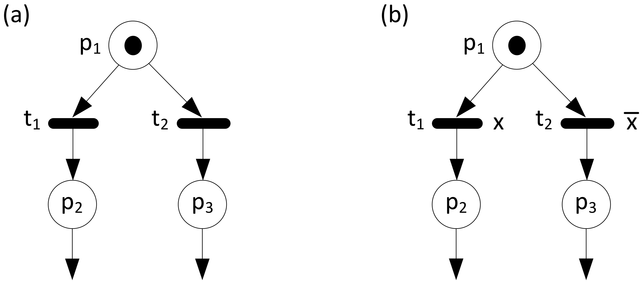
The above papers [31,41,43] point out a very important problem that occurs during modelling of the Petri net-based system intended for the further hardware implementation. Such an issue is related to the conflicts among the transitions. Since this is a crucial issue in the implementation of the Petri-net based systems in FPGAs, let us look closer at this problem. Petri nets in their classical form (i.e., “ordinary Petri nets”) permit the modelling of a system that may contain so-called “conflicts” among the transitions. Such a situation occurs when two or more transitions have a common (unguarded) input place, and each of those transitions can be enabled. Figure 1a shows an example of a conflict in a Petri-net based system among transitions and .
Clearly, conflicts may lead to the nondeterministic behaviour of the system [44]. This problem can be solved in various ways. There exist two main ideas that permit elimination (or avoidance) of conflicts in the modelled design. The first one involves the transformation of the structure of the net [45]. Obviously, such a modification can be a real challenge, especially in the case of relatively complex systems specified by a Petri net. The second solution is based on the application of the special classes of Petri nets (extensions of the ordinary nets) [14,18,46], such as interpreted Petri nets (or just interpreted nets). Since interpreted nets are used in this paper to model the control part of the cyber-physical system, let us briefly discuss their main properties, starting with the resolution of conflicts in the system (please refer to Section 3 for formal definitions and notations related to the interpreted Petri nets).
In general, interpreted Petri nets utilise additional input and output signals, which are associated with the transitions and places of the net, respectively. Those signals are used for communication of the system with the environment, but can also be applied for conflict resolutions in the net. Consider the part of the net shown in Figure 1b. The conflict among transitions and is resolved by the binary input signal , which is associated to both transitions. Once , transition is enabled and it can fire. In the opposite case, when , transition is enabled. Interpreted nets are widely used in modelling of real-life systems, such as concurrent controllers, control systems or cyber-physical systems. However, they are not standardised and there are various definitions of interpreted nets in the literature [44,47,48].
In this paper we will follow interpreted Petri nets, shown in [49], that are live and safe, with binary input and output signals (see Section 2 for details). Such nets are especially applicable in the modelling of systems oriented on the hardware realisation, such as microprocessors [50] or field programmable gate arrays (FPGAs) [49]. Moreover, interpreted nets can be used in the modelling of reconfigurable systems [51]. The latest FPGAs offer a very interesting technique, called dynamic partial reconfiguration. In short, this method permits for the modification of the functionality of the system without stopping the device. Such a property is especially useful in the case of concurrent systems which execute tasks that cannot be interrupted or stopped [51].
Finally, let us discuss the existing design methods of the control part of cyber-physical systems specified by a Petri net and oriented towards implementation in the FPGA. A technique shown in [10] proposes a Petri-net-based specification of cyber-physical systems. In particular, the technique is dedicated to the control of the direct matrix converter with space vector modulation (SVM) and transistor commutation. The presented method utilises the main properties of Petri nets, including verification and analysis of the system. Moreover, the adequate Verilog codes of selected modules are shown. The proposed idea is oriented towards the implementation of the system in programmable devices (in particular, Xilinx FPGA is used). Unfortunately, the technique is strictly oriented towards the control of direct matrix converters and it cannot be applied to any other Petri net-based cyber-physical systems. Moreover, ordinary Petri nets are applied, and the paper does not consider inputs and outputs in the Petri net-based specification of the system (they are included in the further stages of the design).
Another Petri net-based approach oriented towards implementation in the FPGA is shown in [52]. The method also deals with direct matrix converters (as a case-study example), but, contrary to the previously described idea, the detailed design flow is presented. The technique heavily focuses on the verification aspects of the control part of the Petri net-based cyber-physical system. Formal verification and analysis methods are described in detail. Moreover, software simulation and hardware validation of the system is considered. However, the presented descriptions are very general. The paper does not deal with the algorithms that permit the splitting (decomposing) of the system, nor are code templates presented or discussed. Moreover, the proposed technique is mainly oriented towards implementation of the direct matrix converters (i.e., application of a coordinate rotation digital computer, CORDIC method).
To summarise the discussion above, it can be noticed that there are three main issues related to the implementation of the Petri net-based system in the FPGA device. The first one is linked to the conflict resolution in the modelled net and the deterministic behaviour of the system. The second problem refers to the additional conversions and modifications of the specification of the system. The existing solutions often require transformations of the model to other formats or notations. Finally, several techniques are limited to the particular architecture or specification language (e.g., PNML). Therefore, proper modelling of the Petri net-based system for the further realisation in the FPGA device seems not to be a trivial task and very often requires advanced, specialist knowledge. The above issues and limitations are the main motivation for the methods shown in this work.
This paper proposes two design techniques of the Petri-net based systems oriented towards further implementation in the FPGA device. The first one is based on the behavioural description of the system, while the second one involves decomposition of the design into the sequential automata. Both methods are based on the application of the interpreted Petri nets. Such a choice has two main advantages: it permits for easy resolution of conflicts in the system, and additionally allows for the description of the external input and output signals used for communication with the external blocks of the design. Although the presented methodologies are mainly dedicated to the specification of the control part of cyber-physical systems, they can be successfully applied in the modelling of similar systems (such as concurrent controllers).
The main novelty and contributions of the paper can be summarised as follows:
- Proposition of the design flow that is based on the behavioural description of the control part of the cyber-physical system, oriented towards implementation in an FPGA.
- Proposition of the design flow that applies the modular description of the control part of a cyber-physical system (based on the decomposition into sequential automata), oriented towards implementation in the FPGA.
- Proposition of two novel decomposition and synchronisation algorithms for the control part of a CPS specified by an interpreted Petri net, oriented towards further implementation of the system in the FPGA.
- Proposition of descriptions of both presented techniques with the Verilog hardware description language with adequate templates and examples.
- Illustration of the proposed techniques by a real-life case study example of a multi-robot cyber-physical system.
3. Main Notations and Definitions
This section introduces the main notations and definitions used in the paper [14,16,17,18,19,20,22,23,29].
Definition 1.
Petri net: A Petri net is a tuple:
whereis a finite set of places,is a finite set of transitions,is a finite set of arcs, is an initial marking.
Sets of input and output places of a transition are defined as: , , while sets of input and output transitions of a place are denoted as: , .
Definition 2.
Marking: a markingof a Petri net Pis defined as a subset of its places:. A place that belongs to a marking is called a marked place. A marked place holds a token.
Definition 3.
Liveness: a Petri net is live if from any reachable marking it is possible to fire any transition by a sequence of firings of other transitions.
Definition 4.
Safeness: a place of a Petri net is safe if a place holds no more than one token at any reachable marking.
Definition 5.
Interpreted Petri net (interpreted net): an interpreted Petri net is a live and safe Petri net, defined as a six-tuple:
whereis a finite set of binary inputs andis a finite set of binary outputs,. Clearly, (2) is an extension of (1), such that values from the setare associated with the transitions, while outputs from the setare related to the places of IPN.
Definition 6.
Enabled transition: a transition is enabled if all its input places contain a token.
Definition 7.
Transition firing: a transition in the interpreted net is fired if and only if it is enabled, and all its associated input values (from the set ) are fulfilled. The firing of a transition adds a token to each of its output places, and removes a token from each of its input places.
Definition 8.
State machine: a state machine is a Petri net for which every transition has exactly one input place and exactly one output place, i.e., .
Definition 9.
State Machine Component (S-component): a state machine component of an interpreted Petri net is a subnet:
of IPN such that: is a state machine, , , ,, , and has exactly one token in initial marking.
Definition 10.
State machine decomposition (S-decomposition): a state machine decomposition of an interpreted Petri netis a set such that:
- each componentis an S-component,
- each placebelongs to exactly one component .
If place exists in more than one component, it is replaced in all remaining components except one by a non-operational place, denoted as NOP.
Definition 11.
Incidence matrix: an incidence matrix of an interpreted Petri net with
columns and rows is an of integers is given by:
Definition 12
. Place invariant (p-invariant, s-invariant): place invariant of an interpreted Petri net is a nonnegative integer vector such that:
where is an incidence matrix of . Each value of corresponds to a place of the net. The set of places that refers to non-zero values of is called its support.
4. The Proposed Design Flows
Two design techniques of the Petri net-based control part of cyber-physical systems are proposed in this section. The first one is based on the behaviour of the system, while the second involves decomposition of the Petri net into sequential automata (state machine components) [53]. Let us underline that both methods permit for implementation of the system in the FPGA device [51,54]. The selection of the particular technique is strictly dependent on the assumptions and aims of the prototyped design. For example, the first method permits relatively easy description and implementation of the system in the FPGA, but it does not allow for modifications, nor further re-configuration of the device. On the contrary, the second technique involves decomposition of the system, but also permits for optimisation of the achieved sequential automata, or even for partial reconfiguration of the implemented system (under certain assumptions, e.g., additional splitting of the decomposed net into static and dynamic part, see [51] for details).
4.1. Design Flow Based on the Behaviour of the System
The first of the proposed techniques is based on the behavioural description of the system. The proposed design flow consists of the following steps:
- Specification (modelling) of the control part of CPS by an interpreted Petri net.
- * Verification of the Petri net-based model at the specification stage (optional).
- Behavioural description of the Petri net-based system in Verilog HDL.
- * Validation (software simulation) of the design (optional).
- Logic synthesis, logic implementation, and physical implementation in an FPGA.
Let us briefly present each of the above steps, paying special attention to the essential, third step of the flow. Note that two of the above steps (verification and validation of the control part of the CPS) are marked as optional, however it is highly recommended to perform verification and validation of the system. Let us also point out that the design example based on the above flow is shown in Section 5.
4.1.1. Specification of the Control Part of CPS by an Interpreted Petri Net
At the beginning, the control part of the CPS is formally specified by an interpreted Petri net [55,56,57,58,59]. Such a model is created based on the informal description of the system. The control part of the CPS is specified by places and transitions of the net, according to the Equation (2). Additionally, an interpreted Petri net permits for binary input and output signals that are associated with the transitions and places, respectively. Those signals permit for communication of the control part with the remaining elements of the cyber-physical system. Moreover, (if needed) input signals can be used for conflict resolution in the net (recall Figure 1b).
4.1.2. Verification of the Petri Net-Based Model at the Specification Stage
Once the system is specified, it can be formally verified at the early specification stage. In particular, liveness and safeness are crucial properties, since the modelled control part of the CPS should fulfil all the conditions of interpreted Petri nets. There are several methods and tools that permit verification and analysis of Petri net-based systems [22,24,60,61,62,63]. The most popular are based on the linear algebra technique or involve computation of the reachability tree. Moreover, advanced analysis of the sequentiality and concurrency relation in the Petri net can be performed [16].
4.1.3. Behavioural Description of the Petri Net-Based System in Verilog HDL
This is an essential step of the presented design flow. The behaviour of the Petri net-based specification of the control part of the CPS is described in the Verilog language [64,65]. This process can be divided into four stages:
- description of the main module;
- description of transition firings;
- description of places;
- description of outputs.
At the beginning, the initial structure of the main module is described. Based on the system specification, the names of module, input and output signals are defined. Moreover, the set of transitions and places are defined. Listing 1 shows the template of such descriptions.
| Listing 1. Template of the module description in Verilog. |
 |
The first line specifies the name of the module, as well as declaring the input and output signals. Such values are strictly related to the explicit declarations of outputs and inputs (lines 2–4). The value Y refers to the number of binary output signals, while X denotes the number of binary input signals in the interpreted Petri net. Note that such ports can be named explicitly (i.e., start, stop, etc.) however to clarify the presentation we will follow traditional notations Y and X. Also declared are two additional input ports clk and reset. These signals are necessary due to the realisation of the system in an FPGA. The first one refers to the clock oscillator, while the second permits a reset of the system to its initial state. Furthermore, the sets of transitions and places of the interpreted Petri net are declared within lines five and six, respectively. Value T refers to the number of transitions (|T|), while P means the number of places (|P|) in the net. Three subsequent sections (description of transitions, places, and outputs) remain empty at this moment. The description of the module is finalised by the endmodule statement.
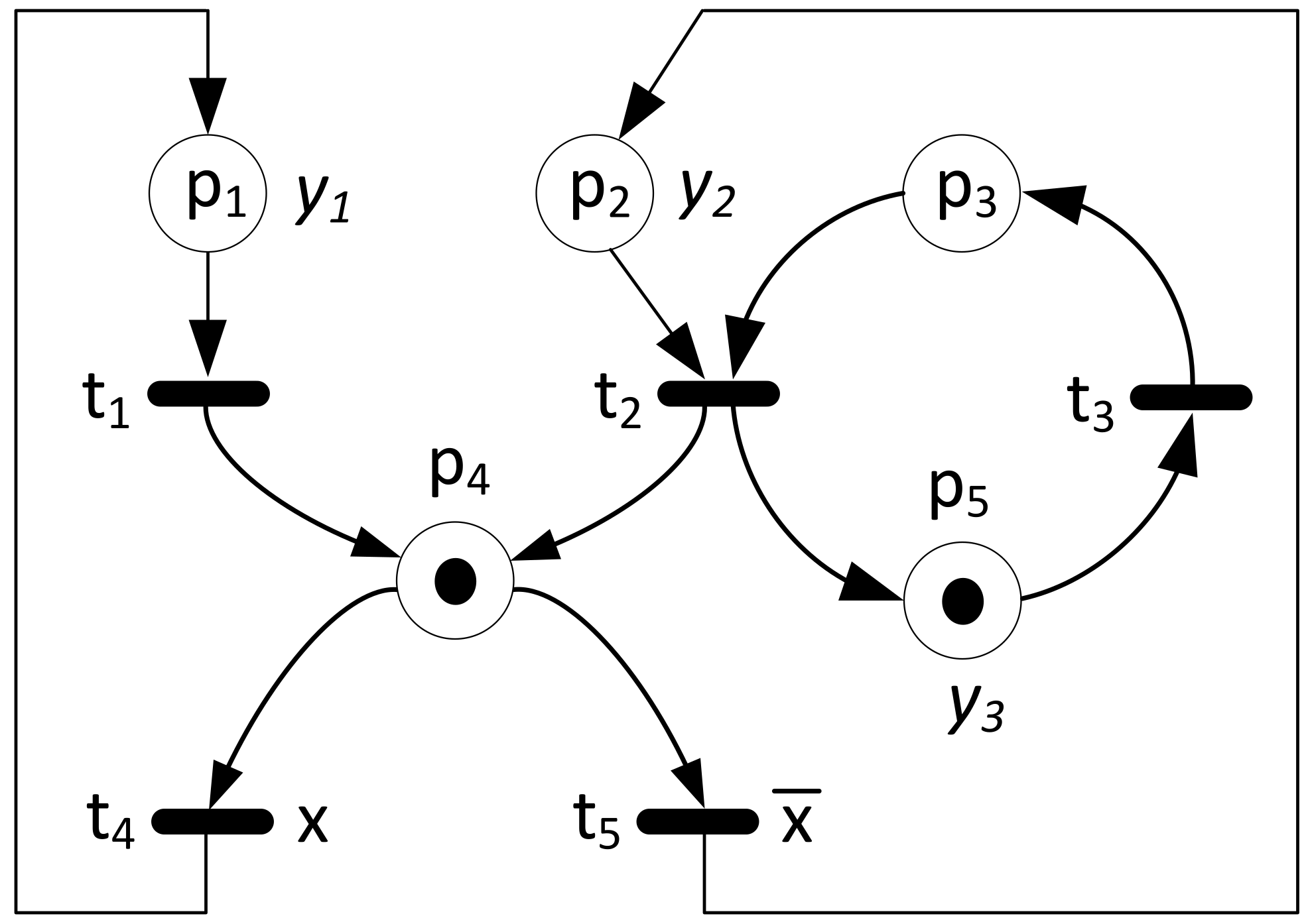
At the next stage, the transition firings are described. The behaviour of each transition is outlined as a logical conjunction of its input places (set P) and related conditions (set X). This description is realised by a continuous assignment (assign statement). Let us illustrate it by an example. Consider the interpreted Petri net shown in Figure 2.
There are five transitions in the presented interpreted Peri net. Listing 2 shows the description of transition firings for this Petri net. Note that there is a conflict between transitions and , that is resolved by an input signal . Furthermore, there are two input places of , therefore a logical conjunction of those places is assigned to this transition.
| Listing 2. Description of transition firings in Verilog. |
 |
The third step includes the behavioural description of places. The presented solution is based on the procedural assignments within always block. It is assumed that the system is oscillated by a positive (rising) edge of the clock (clk) signal. Moreover, the asynchronous reset signal allows for zeroing the system and returns it to the initial state (initial marking). The description of each place is formed as a logical disjunction of conditions that permit holding a token at the particular place, and all input transitions of this place. In particular, the condition that allows keeping a token is formed as a conjunction of the place together with negations of all its output transitions. Let us explain the above by an example shown in Figure 2. Listing 3 presents the description of places for this net.
There are five places in the net. The description of place (line 6) is outlined as a logical disjunction of a condition that permits holding a token at this place (in particular, it is formed as a conjunction of and negation of ) with all its input transitions (in this case there is only one, transition ). Places and are described in a very similar way. However, place has two input and two output transitions. Therefore, the description of this place includes the conjunction of variables that allow the token to be kept with two input transitions (, ). Note that active signal reset permits the return of the system to the initial marking.
| Listing 3. Description of places behaviour in Verilog. |
 |
Finally, outputs of the control part of the CPS are described. Since they are related to the particular places of the net, continuous assignments are applied. Listing 4 shows an exemplary description of outputs for the net shown in Figure 2. Note that assignments for all outputs are combined in one line, but alternatively, they can be explicitly written (within three lines, each for a single output).
| Listing 4. Description of outputs in Verilog. |
 |
4.1.4. Validation of the System (Software Simulation)
Once the control part of the cyber-physical system is described in Verilog HDL, it can be validated. Such an operation is usually performed within the tool that permits the description of the system in the hardware description language. The particular inputs are stimulated by user-defined values, while the outputs are obtained based on the functionality of the design.
It should also be noted that validation is often confused with verification of the system (the second step of the presented design flow). In the presented considerations, we followed the IEEE standard 1012–2016 [66], according to which validation permits the evaluation of whether the design satisfies the specified requirements. In contrast, verification refers to the examination of the design, which determines whether it is properly modelled.
4.1.5. Logic Synthesis, Logic Implementation, and Physical Implementation in an FPGA
Finally, the system is ready for realisation in the FPGA. The final implementation is strictly connected with the vendor of the destination device. In the presented flows, we will follow Xilinx guidelines [67], however this process is very similar for other vendors. Firstly, the design is logically synthesised and logically implemented. The first operation permits translation of the Verilog-based description into the gate level representation, while logic implementation translates, maps and adjusts the system to the particular device. The physical device can be configured with the configuration file (called bit-stream). Once the FPGA is programmed, the designer is able to validate the control part of the CPS in the real environment. Since a field programmable gate array is a reprogrammable device, any detected errors and malfunctions may be easily corrected and implemented again. Note that in such a situation the complete design path ought to be repeated.
4.2. Design Flow Based on the Decomposition of the System
The second technique involves decomposition of the control part of the CPS into state machine components. Each component is further described as a sequential automaton in the Verilog HDL. The proposed design flow consists of the following steps:
- Specification of the control part of the CPS by an interpreted Petri net.
- * Verification of the Petri net-based model at the specification stage (optional).
- Decomposition of the model into state machine components.
- Synchronisation of decomposed components (for further implementation in FPGA).
- * Optimisation of components (optimisation of sequential automata).
- Description of the decomposed automata in Verilog HDL.
- * Validation (software simulation) of the design (optional).
- Logic synthesis, logic implementation, and physical implementation in an FPGA.
The presented design flow includes eight main steps. Similar to the technique shown in the previous subsection, there are optional stages. However, besides verification and validation of the design, there is a possibility of additional optimisation (or modification) of the decomposed components. Let us explain the above flow in more detail. Since steps 1, 2, 7 and 8 are very similar to the stages shown in Section 4.1, we mainly focus on the remaining points of the flow.
4.2.1. Specification of the Control Part of the CPS by an Interpreted Petri Net
This step is executed in the same manner as in the behavioural description of the system. The control part of CPS is specified by an interpreted Petri net. Inputs of the model are assigned to transitions, while outputs to places of the net.
4.2.2. Verification of the Petri Net-Based Model at the Specification Stage (Optional)
The model of the control part of the CPS can be formally verified at the specification stage. Since Petri nets are widely supported by various verification methods and tools, this process may involve several aspects, depending on the designer needs.
4.2.3. Decomposition of the Model into State Machine Components
This is the crucial step of the flow. Decomposition divides the system into the smaller components. In particular, the proposed design flow is based on the S-decomposition of the system. According to Definition 10, such an operation splits the interpreted Petri net into state machine components. There exists several decomposition algorithms, based on the linear algebra technique (place invariant computation), reachability graph analysis, or concurrency graph (or hypergraph) exploration [14,44,49]. Furthermore, the techniques shown in [68] seem to be applicable. However, the ideas are based on the tool chain (which additionally uses third-party software), and a certain conversion of the specification to the required formats is needed. The authors conducted experimental research but did not provide information about the applied resources (processors, memories, etc.; there is just a mention about “a 9-year old laptop”). It should be also noted that the comparison to the external tools and systems was done “as is”, without considering their technical properties and applied internal mechanisms.
The method shown in this paper is based on linear algebra, however any other S-decomposition technique can be used instead. The method searches for the invariants that fulfil Equation (5), and additionally form proper SMCs, according to Equation (3). In particular, the proposed decomposition algorithm consists of the following operations:
- Initialisation:
- (a)
- form the set of S-components that form S-decomposition of the interpreted Petri net (initially empty);
- (b)
- form the unit matrix , where is initially an identity matrix, and is an incidence matrix of , formed according to (4);
- (c)
- set counter variable c of non-operational places to zero: .
- For each transition (column of matrix ):
- (a)
- find row pairs that annul the -th column of and append it to matrix ;
- (b)
- delete rows of whose intersection with the -th column is not equal to 0;
- (c)
- reduce redundant rows of (i.e., rows that binary cover to the other ones).
- For each row of whose all elements contain 0:
- (a)
- obtain support of invariant from matrix ;
- (b)
- construct subnet of such that:
- =;
- is associated to any };
- is associated to any };
- (c)
- if forms a proper S-component (according to Definition 9 and Equation (3)):
- for each place such that p belongs to the other S-component :
- -
- replace or by a non-operational place ;
- -
- for all associated to : ;
- -
- increase the counter of non-operational places: ;
- add S-component to the S-decomposition: ;
- (d)
- remove row r from Q.
- Break if all places are covered by S-components , otherwise repeat the procedure from the step 2.
- Finish with information that the interpreted Petri net cannot be decomposed.
The above algorithm permits the obtaining of the S-decomposition of the interpreted Petri net, and is based on the classical method initially shown in [69]. However, let us emphasise the point that the algorithm presented in [69] computes place invariants, and does not permit the obtaining of S-decomposition, nor S-components of the net. Therefore, additional transformations, sub-net constructions and verifications are required (steps 3–5). Moreover, the presented method stops computation once the decomposition is found. Note that there is a possibility that the particular interpreted Petri net cannot be decomposed. In such a case, the behavioural design flow ought to be applied.
4.2.4. Synchronisation of Components (for Further Implementation in FPGA)
Once the control part of the CPS is decomposed, it should be properly synchronised. Initially (that is, after the decomposition) each of the obtained S-components forms an independent system. Therefore, proper synchronisation between transitions ought to be assured. In general, such an operation is not a trivial task, especially in case of distributed systems. However, the proposed technique is strictly designed for the FPGA device, and therefore synchronisation of components can be solved by internal signals. Note that the presented solution assumes that the whole control part of the CPS (all the decomposed components) is oscillated by the same clock signal.
The proposed synchronisation algorithm consists in the following steps:
- Initialisation:
- (a)
- form the set of synchronisation signals (initially empty);
- (b)
- set counter variable c of applied synchronisation signals to one: .
- For each transition such that is shared by two or more :
- (a)
- for each input place of transition ():
- if there is already assigned synchronisation signal to :
- otherwise:
- -
- add new synchronisation signal and assign it to ;
- -
- ;
- -
- increase the counter of synchronisation signals: ;
- (b)
- for each component that contains :
- obtain current logical condition that is assigned to ;
- for each :
- -
- if is assigned to : add to the set : ;
- -
- otherwise:
- -
- add to the logical condition : ;
- -
- add to the set .
Let us briefly describe the behaviour of the above method. Firstly, the algorithm searches for the transitions shared among components. For each input place of such transition, a synchronisation signal is added (step 2a). Moreover, this synchronisation signal is assigned to each transition in the other S-components (step 2b). Additionally, sets of binary input and output signals for each S-component are updated.
4.2.5. Optimisation of Obtained Components (Optional)
The decomposed and synchronised control part of the cyber-physical system is ready for description in the Verilog language. However, there is a possibility for additional modifications of obtained modules since each of the S-components form a sequential automaton. Therefore, it can be transformed and optimised (for example, into a microprogrammed control unit). The advanced methods of optimisation of sequential automata designed for implementation in an FPGA can be found in [35,70,71,72].
4.2.6. Description of the Decomposed Automata in Verilog HDL
The proposed description of the decomposed control part of the CPS utilises a modular approach. Each of the S-components is outlined as a finite state machine (Moore automaton). The top-level module (at the highest level of hierarchy) includes instantiations of all decomposed components. The process is split into two main steps:
- description of the top-level module;
- description of the decomposed S-components.
Firstly, the top-level module is described. Besides declarations of input and output signals of the control part, this module contains instantiations of decomposed S-components. Moreover, synchronisation signals among the SMCs are declared, as well. Listing 5 shows the template of the top-level description in Verilog HDL.
Next, each S-component is specified as an independent Verilog module. The description of the S-component can be divided into six main blocks:
- declaration of the module;
- * declaration of automaton registers;
- * encoding of register states;
- * description of the functionality of Moore automaton;
- description of transition functions;
- description of outputs.
| Listing 5. Template of the top-level module description in Verilog. |
 |
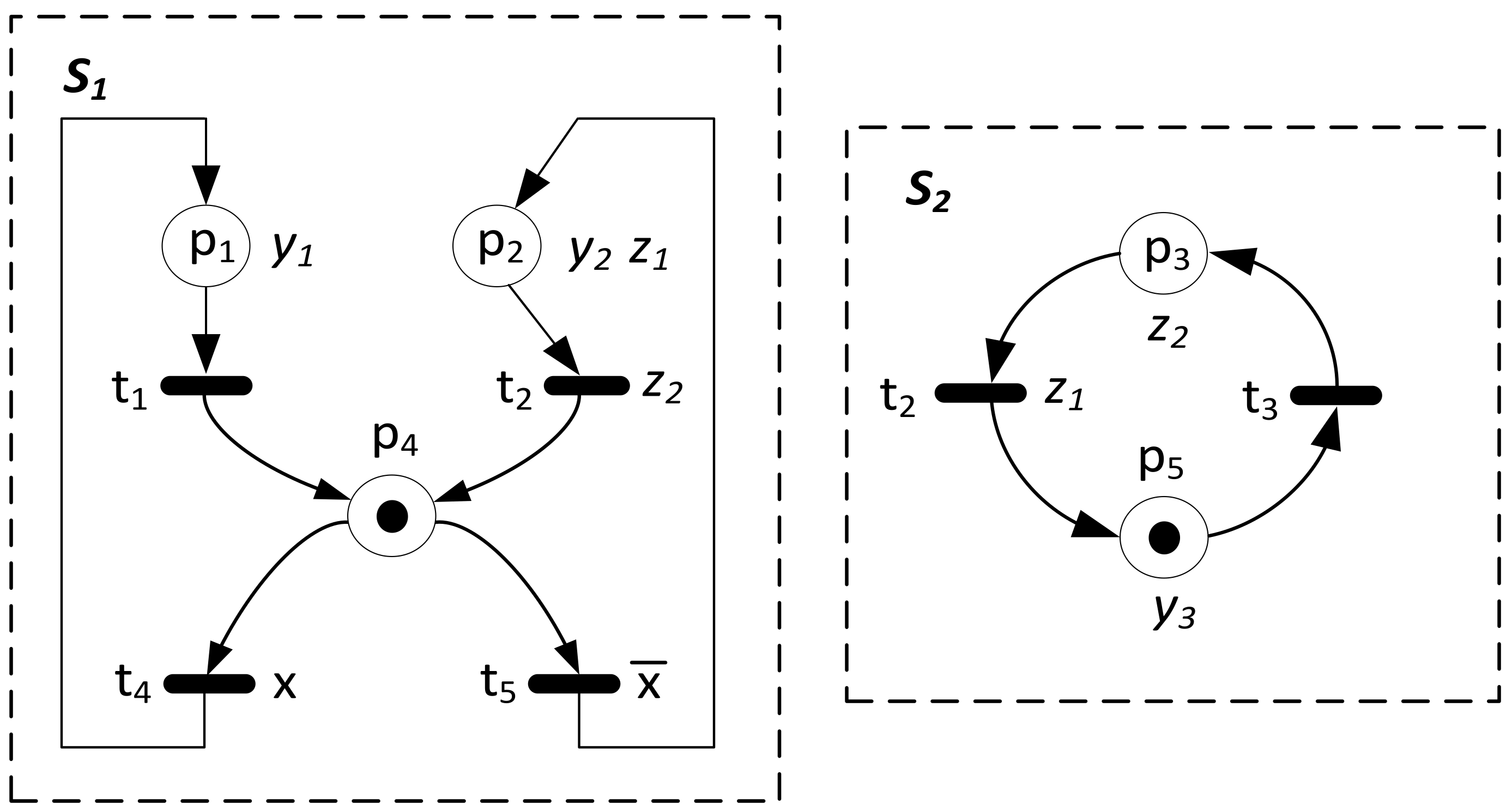
Three of the above steps (marked with an asterisk) are almost the same for each component; only the size of registers may vary. Let us explain the description of an S-component by example. Recall the interpreted Petri net N1 (Figure 2). Figure 3 shows the decomposed and synchronised control part of this CPS.
The presented control part was decomposed according to the algorithm shown in Section 4.2.3 into two S-components ( and ). Further synchronisation resulted in supplementation of components by two additional signals (,). Listing 6 presents the description of the first S-component (). Let us briefly describe each block of the above description. It should be pointed out that the general rules applied in the proposed description of Moore automaton are strictly based on the Xilinx guidelines [73].
To begin, the module name, input and output ports are declared. Note that is declared as an output, since it is associated to place (input place of shared transition). Analogously, is specified as an input and it is assigned to the shared transition .
At the subsequent block of the description automaton registers for the current and next state are declared. The number of required registers is strictly related to the number of places in the component, and can be simply expressed as:
where is the number of places in the particular S-component.
The next block refers to the encoding states of the component. Note that the proposed flow strictly follows the initial names and notations, thus states of automaton refer to the places of the S-component. In the presented example, there are three states (places): . The designer is able to encode states according to need.
The fourth part of the description outlines the behaviour of the Moore automaton. The clock signal is used for changing states (according to the transition functions), while asynchronous reset allows returning to the initial marking. This block remains unchanged for each S-component.
Transition functions are specified in the fifth block of the description. This section involves procedural always block. The sensitivity list contains state variable and all input signals from the set (that is, a list of all inputs assigned to transitions in this S-component, including synchronisation signals). The selection of the next state is expressed by the case statement, and simply describes the behaviour of Moore automaton.
Finally, the last block outlines outputs of the module, including synchronisation signals associated with the places of the S-component. This description is realised by the continuous assignments.
| Listing 6. Template of the module description in Verilog. |
 |
4.2.7. Validation of the Design (Optional)
The decomposed control part of the CPS can be validated by the software simulation. Moreover, each S-component can be checked as an independent module. Since all components are oscillated by the same clock signal, the obtained results should be the same as in case of the behavioural validation of the design (cf. Section 4.1.4).
4.2.8. Logic Synthesis, Logic Implementation, and Physical Implementation in an FPGA
This step is executed in exactly the same manner as is presented in Section 4.1.5. The decomposed system is logically synthesised and logically implemented. The resulting bit-stream is further sent to the destination FPGA device.
5. The Case-Study Example of the Proposed Design Flows
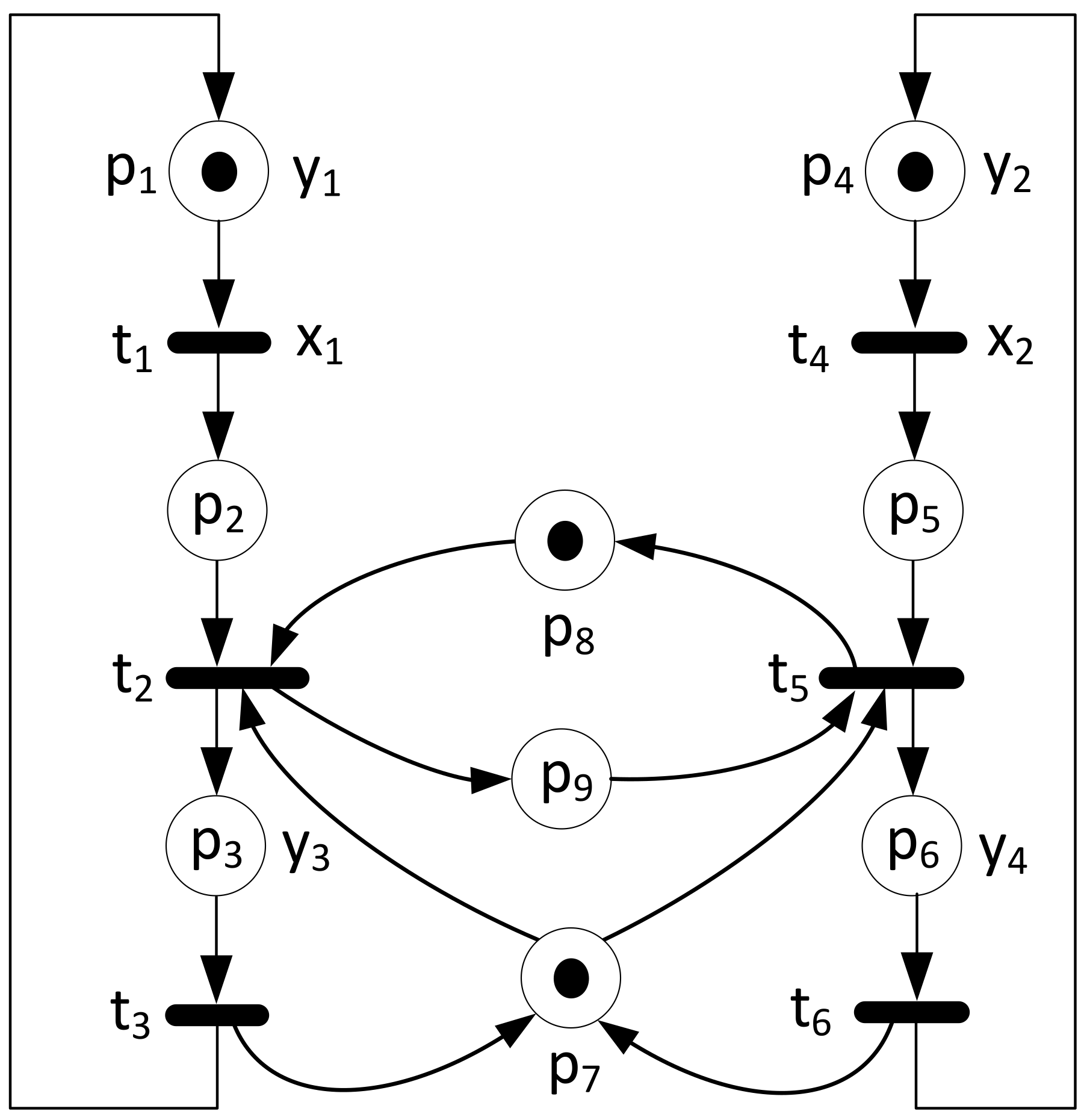
This section illustrates the proposed design flows by a real-life example of the control part of the CPS. Consider the interpreted Petri net shown in Figure 4 that describes the cyber (control) part of a multi-robot assembly system. The specification is a slightly modified version of the system initially presented in [74]. In particular, the net was supplemented by the input and output signals (sets and ). There are six transitions and nine places in the net. Its behaviour is additionally controlled by two input signals: ,. Moreover, there are four output signals: ,. Let us briefly describe the functionality of the system. Two robot arms perform tasks inside and outside the common workspace. In particular, the operations related to the first arm are specified by places ,, while places , are related to the second arm. Outputs and are associated with actions executed outside the common workspace, thus both arms can perform them at the same time. However, operations related to outputs and are realised inside the common workspace, and they cannot be executed simultaneously.
The collision-free movements of robot arms are assured by mutual exclusion. In particular, places are used in order to secure the proper functionality of the control part, by adequate distribution of a token. The first arm of the robot may access the common workspace if place is marked. Otherwise, place holds a token, and the second arm of the robot is able to perform tasks in the common workspace.
The presented Petri net is live and safe. This means that there are no deadlocks in the system, and each place holds no more than one token (at any reachable marking). Note that the above properties are crucial, since liveness and safeness are necessary conditions for interpreted Petri nets.
Since specification and verification of the Petri net is already done, let us now proceed to the remaining steps of the proposed design flows, starting with the behavioural description of the system. Listing 7 shows the Verilog description of the presented control part of the CPS. According to the method presented in Section 4.1.3, initially the module, together with input and output signals is specified (the first four lines of the code). Moreover, 9 places and 6 transitions are declared (lines 5–6).
| Listing 7. The behavioural description of the control part of a multi-robot system in Verilog. |
 |
The transition firings are realised by six continuous assignments (lines 7–12). Each transition is described as a logical conjunction of its input places and associated input signals (if any). For example, transition is outlined as a conjunction of input place and input (which is associated to ), while is described as a conjunction of three of its input places: .
The description of places (lines 13–28) is based on the procedural assignments realised by the always block. The asynchronous reset zeroes the control part of the CPS to its initial state (marking). Each place is outlined as a logical disjunction of conditions that either allows holding a token at its current place (that is, output transitions of this place are not enabled), or firing input transitions from this place. For example, place is described as a logical disjunction of the conditions: (all output transitions are not enabled), , . It means that is active if either a token is already within this place, or transition is enabled, or transition is enabled. Similarly, the remaining places are described.
Finally, the output signals are outlined, as continuous assignments of places. There are four outputs in the presented example. In this particular case, the single assignment was used (line 29), however each output can be outlined separately.
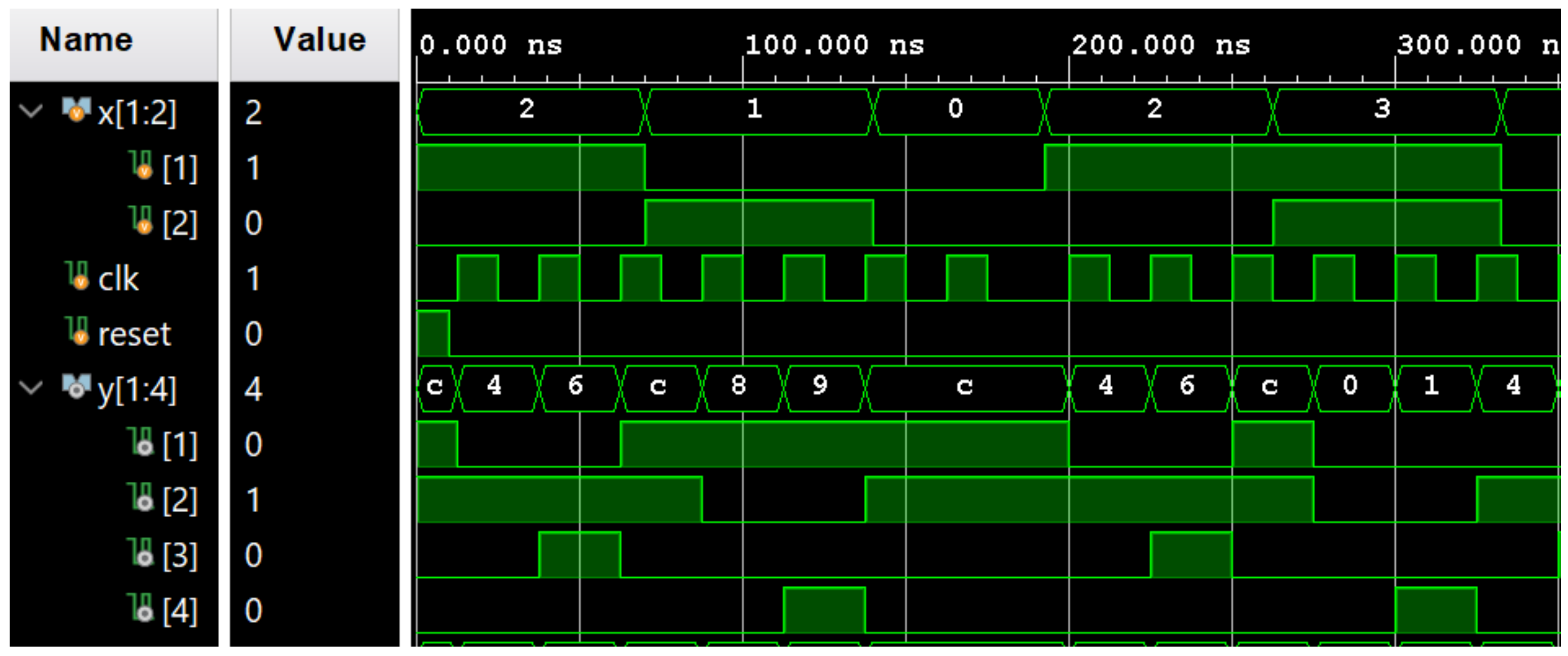
The subsequent step of the proposed design flow involves validation of the control part. The simulation was performed within Xilinx Vivado 2021.1 [75]. Figure 5 shows the obtained validation result.
The values for input signals were stimulated (the clock signal was set to 40 MHz = 25 ns), while the output signals were obtained according to the functionality of the design. The performed validation confirmed proper functionality of the control part. It can be noted that all of the outputs behave according to the assumed informal specification of the multi-robot system.
Once the validation confirms proper functionality, the control part of the CPS was implemented in an FPGA. In the presented example the Xilinx device xc7a100T (Artix7 family) was used. The logical synthesis and logical implementation finished with success, confirming the proper behavioural description of the control part in the Verilog language. Table 1 shows the utilisation of the FPGA resources. It can be noticed that the implemented control part of the multi-robot system consumes just a fraction of the FPGA area. Moreover, the results achieved confirm the described system. Nine places of the specified system directly refer to the number of declared registers in the Verilog code and–finally-utilised registers of the device. Similarly, the number of input/output blocks is exactly as expected (in total eight: four inputs and four outputs). Finally, the logic of the control part (including description of transitions and equations of places) was implemented within seven look-up tables (LUTs).
Let us now move on to the second of the proposed flows. The control part of a multi-robot system will be decomposed, synchronised, and described in Verilog HDL, and implemented in the FPGA device.
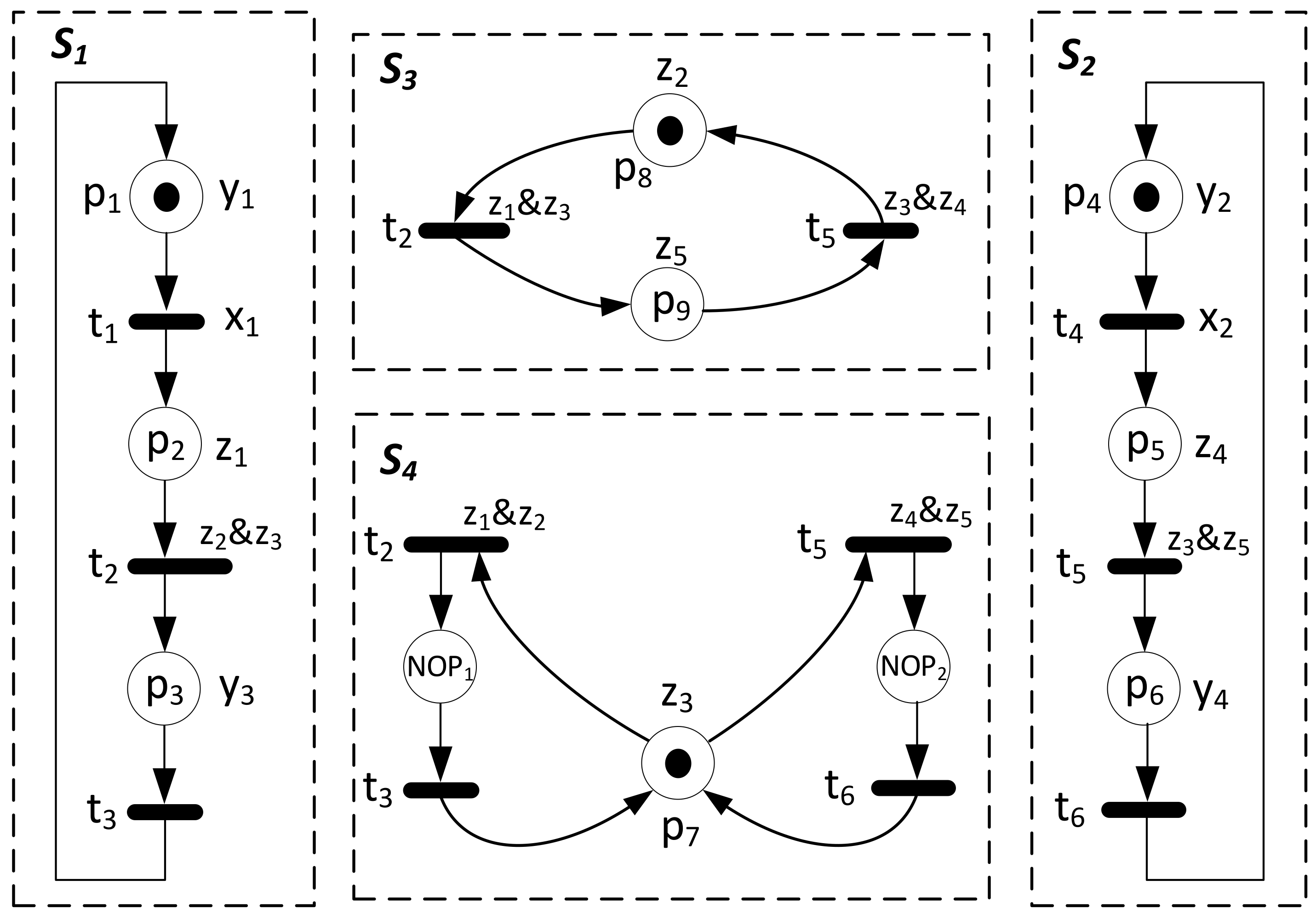
The first two steps of the design flow are exactly the same as in case of the behavioural flow. Decomposition and synchronisation of the control part were executed according to the algorithms shown in Section 4.2.3 and Section 4.2.4, respectively. Figure 6 presents the decomposed and synchronised control part of the multi-robot assembly system.
The presented system was decomposed into four S-components: . Three components ( contain three places, while the remaining one () consists of two places. Note that contains two non-operational places: replaces (which already belongs to ), and replaces (which is included within ).
Further synchronisation of the system resulted in five signals: , which are used for proper synchronisation of two shared transitions: and . The first one () is shared among three components: , while exists in .
Listing 8 illustrates the description of the top-level module in the Verilog language. Declarations of input and output ports (lines 1–4) are exactly the same as in the case of the behavioural description. Synchronisation signals are declared within line 5, while instantiations of particular S-components are invoked in lines 6–9.
| Listing 8. Description of the top-level module of the decomposed control part of a multi-robot. |
 |
Description of the S-component is presented in Listing 9. There are three output and five input signals in the module. Three of them refer to the synchronisation signals, one output () and two inputs (). Component consists of three places, therefore registers which are used for encoding states. Descriptions of transition functions simply set the values of the next state, according to the possible conditions. Finally, outputs are generated depending on the current state of the automaton.
| Listing 9. Description of of the decomposed control part of a multi-robot system. |
 |
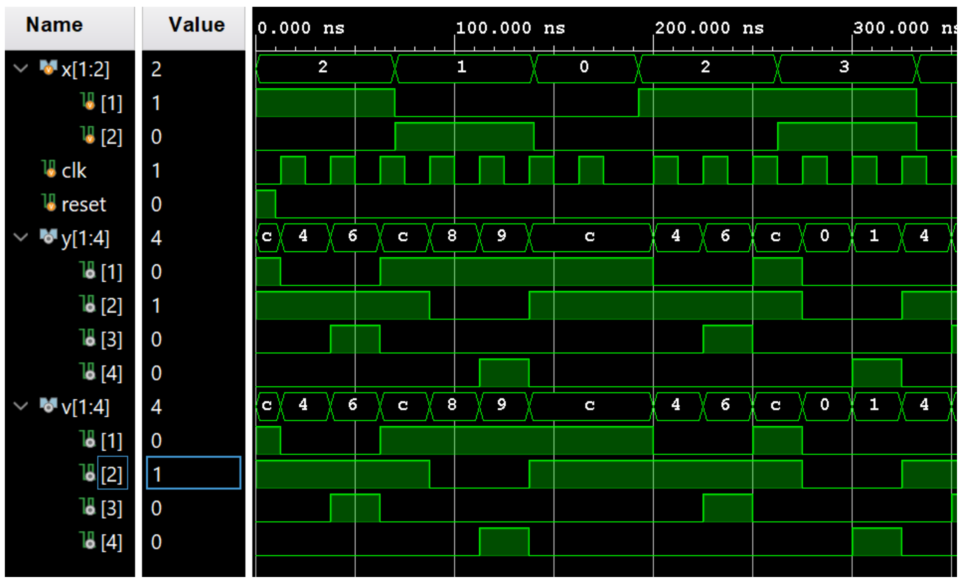
The descriptions of the remaining three components are executed in exactly the same way. The complete Verilog code of all decomposed S-components can be found in the Appendix A. Figure 7 shows the validation results of the decomposed control part of the multi-robot system. Additionally, the simulation results include the behavioural description of the system. Therefore, the functionality of both descriptions can be easily compared. In particular, signals ““ are generated by the behavioural description, while signals ”” are the result of the modular (decomposed) description of the system. It can be seen that results from both models (behavioural and decomposed) are exactly the same.
Finally, the decomposed control part of the multi-robot system was implemented in the FPGA. In particular, the same device was applied as in the case of the behavioural flow. Table 2 displays the utilisation of the FPGA device. It can be seen that the decomposed system used a very similar portion of the device as the behavioural description. An interesting fact is related to the number of utilised logic elements (LUTs) and registers (flip-flops). Both descriptions lead to almost the same results (7/8 LUTs, 9 FFs). However, optimisation of the S-components obtained during the SM-decomposition (cf. Section 4.2.5) may result in decreasing the utilised resources.
6. Conclusions
This paper proposes two design flows for the control part of a cyber-physical system intended for implementation in the FPGA device. The first technique is based on the behaviour of the system, while the second method applies decomposition into sequential automata (S-components). Both ideas involve synthesisable descriptions in the Verilog language. The presented design flows are explained by the real-life example of the multi-robot assembly system. Let us underline that both design techniques shown in the paper are novel. Obviously, notations or descriptions may be similar to the existing solutions, but general concepts, including particular Verilog design styles, are the result of the author’s years of experience with Petri nets and FPGAs. The first of the presented methods applies a direct description of the control part of the cyber-physical system in the Verilog language, with the possibility of further implementation in the FPGA. The second technique is based on the splitting of the initial model into state machine components. Adequate decomposition and synchronisation algorithms (strictly oriented towards the further application in the programmable device) are proposed. Both presented design flows are supplemented by the code templates. Moreover, detailed explanation by a real-life multi-robot assembly system is presented. It should be noted that the obtained validation results of the system designed by both flows are exactly the same. Furthermore, the utilisation of the FPGA device is similar. However, modules obtained during the SM-decomposition of the system can be optimised in order to reduce the number of utilised logic elements (LUTs, flip-flops). Moreover, obtained sequential automata are applicable in the dynamic partial reconfiguration of the system (cf. [51] for details).
The scope of the proposed techniques covers a wide range of cyber-physical systems where FPGA devices are applicable, including concurrent control systems [14,31,56], power grids and energy systems [10,52], manufacturing and production systems [49,51], and others. On the other hand, the main limitation of the proposed techniques is related to the applied specification formalisms. Both design flows are based on Petri nets and Verilog language, thus the presented solutions can be embarrassing for designers that are not familiar with this methodology and/or this hardware language. On the other hand, the presented design flows are presented in detail (with templates of Verilog codes). Moreover, Petri nets are widely supported by analytic methods and tools, which makes possible verification at the early (specification) stage. Finally, the presented methodology can be easily adopted to other hardware languages (for example VHDL).
Further research includes optimisation of the decomposed S-components in order to reduce the utilisation of the FPGA resources. Moreover, development of alternative decomposition techniques is considered.
Funding
This work is supported by the National Science Centre, Poland (grant number 2019/35/B/ST6/01683).
Conflicts of Interest
The authors declare no conflict of interest.
Appendix A
Listings A1–A3 present the Verilog source codes of S-components , , of the decomposed control part of the multi-robot assembly system shown in Section 4.
| Listing A1. Description of of the decomposed control part of a multi-robot system. |
 |
| Listing A2. Description of of the decomposed control part of a multi-robot system. |
 |
| Listing A3. Description of of the decomposed control part of a multi-robot system. |
 |
References
- Lee, E.A.; Seshia, S.A. Introduction to Embedded Systems: A Cyber-Physical Systems Approach, 2nd ed.; MIT Press: Cambridge, MA, USA, 2016. [Google Scholar]
- Hahanov, V. Cyber Physical Computing for IoT-Driven Services; Springer: Cham, Switzerland, 2018. [Google Scholar]
- Alur, R. Principles of Cyber-Physical Systems; MIT Press: Cambridge, MA, USA, 2015. [Google Scholar]
- Shamim, S.; Cang, S.; Yu, H.; Li, Y. Examining the Feasibilities of Industry 4.0 for the Hospitality Sector with the Lens of Management Practice. Energies 2017, 10, 499. [Google Scholar] [CrossRef] [Green Version]
- Dey, N.; Ashour, A.S.; Shi, F.; Fong, S.J.; Tavares, J. Medical cyber-physical systems: A survey. J. Med Syst. 2018, 42, 74. [Google Scholar] [CrossRef] [Green Version]
- Huang, D.; Deng, Z.; Wan, S.; Mi, B.; Liu, Y. Identification and Prediction of Urban Traffic Congestion via Cyber-Physical Link Optimization. IEEE Access 2018, 6, 63268–63278. [Google Scholar] [CrossRef]
- Ang, J.H.; Goh, C.; Saldivar, A.A.F.; Li, Y. Energy-Efficient Through-Life Smart Design, Manufacturing and Operation of Ships in an Industry 4.0 Environment. Energies 2017, 10, 610. [Google Scholar] [CrossRef]
- Puliafito, A.; Tricomi, G.; Zafeiropoulos, A.; Papavassiliou, S. Smart Cities of the Future as Cyber Physical Systems: Challenges and Enabling Technologies. Sensors 2021, 21, 3349. [Google Scholar] [CrossRef]
- Garcia, D.A.; Cumo, F.; Tiberi, M.; Sforzini, V.; Piras, G. Cost-Benefit Analysis for Energy Management in Public Buildings: Four Italian Case Studies. Energies 2016, 9, 522. [Google Scholar] [CrossRef]
- Wisniewski, R.; Bazydlo, G.; Szczesniak, P.; Wojnakowski, M. Petri Net-Based Specification of Cyber-Physical Systems Oriented to Control Direct Matrix Converters With Space Vector Modulation. IEEE Access 2019, 7, 23407–23420. [Google Scholar] [CrossRef]
- Canaan, B.; Colicchio, B.; Abdeslam, D.O. Microgrid Cyber-Security: Review and Challenges toward Resilience. Appl. Sci. 2020, 10, 5649. [Google Scholar] [CrossRef]
- Din, F.U.; Ahmad, A.; Ullah, H.; Khan, A.; Umer, T.; Wan, S. Efficient sizing and placement of distributed generators in cyber-physical power systems. J. Syst. Arch. 2019, 97, 197–207. [Google Scholar] [CrossRef]
- Hahanov, V.; Litvinova, E.; Chumachenko, S. Green Cyber-Physical Computing as Sustainable Development Model. In Studies in Systems, Decision and Control; Springer Science and Business Media LLC: Berlin/Heidelberg, Germany, 2017; pp. 65–85. [Google Scholar]
- Wiśniewski, R. Prototyping of Concurrent Control Systems Implemented in FPGA Devices; Springer Science and Business Media LLC: Berlin/Heidelberg, Germany, 2017. [Google Scholar]
- Sirjani, M.; Lee, E.A.; Khamespanah, E. Verification of Cyberphysical Systems. Mathematics 2020, 8, 1068. [Google Scholar] [CrossRef]
- Wisniewski, R.; Wisniewska, M.; Jarnut, M. C-Exact Hypergraphs in Concurrency and Sequentiality Analyses of Cyber-Physical Systems Specified by Safe Petri Nets. IEEE Access 2019, 7, 13510–13522. [Google Scholar] [CrossRef]
- Best, E.; Devillers, R.; Koutny, M. Petri Net Algebra. Springer-Verlag: Berlin/Heidelberg, Germany, 2001. [Google Scholar]
- Giua, A.; Silva, M. Petri nets and Automatic Control: A historical perspective. Annu. Rev. Control. 2018, 45, 223–239. [Google Scholar] [CrossRef]
- Girault, C.; Valk, R. Petri Nets for Systems Engineering: A Guide to Modeling, Verification, and Applications; Springer: Berlin/Heidelberg, Germany, 2013. [Google Scholar]
- Murata, T. Petri nets: Properties, analysis and applications. Proc. IEEE 1989, 77, 541–580. [Google Scholar] [CrossRef]
- Luo, J.; Ni, H.; Zhou, M. Control Program Design for Automated Guided Vehicle Systems via Petri Nets. IEEE Trans. Syst. Man, Cybern. Syst. 2014, 45, 44–55. [Google Scholar] [CrossRef]
- Szpyrka, M.; Wypych, M.; Biernacki, J.; Podolski, L. Discrete-Time Systems Modeling and Verification With Alvis Language and Tools. IEEE Access 2018, 6, 78766–78779. [Google Scholar] [CrossRef]
- Karatkevich, A. Dynamic Analysis of Petri Net-Based Discrete Systems; Springer: Berlin/Heidelberg, Germany, 2007. [Google Scholar]
- Ran, N.; Hao, J.; He, Z.; Seatzu, C. Diagnosability analysis of bounded Petri nets. In Proceedings of the 2018 IEEE 23rd International Conference on Emerging Technologies and Factory Automation (ETFA), Turin, Italy, 4–7 September 2018. [Google Scholar]
- Li, B.; Khlif-Bouassida, M.; Toguyéni, A. On–The–Fly Diagnosability Analysis of Bounded and Unbounded Labeled Petri Nets Using Verifier Nets. Int. J. Appl. Math. Comput. Sci. 2018, 28, 269–281. [Google Scholar] [CrossRef] [Green Version]
- Szpyrka, M.; Biernacka, A.; Biernacki, J. Methods of Translation of Petri Nets to NuSMV Language. In Proceedings of the CEUR Workshop Proceedings, Chemnitz, Germany, 29 September–1 October 2014; pp. 245–256. [Google Scholar]
- Van Der Aalst, W.M.P.; Van Hee, K.K.; Ter Hofstede, A.; Sidorova, N.N.; Verbeek, E.; Voorhoeve, M.M.; Wynn, M. Soundness of workflow nets: Classification, decidability, and analysis. Biol. Cybern. 2011, 23, 333–363. [Google Scholar] [CrossRef] [Green Version]
- Zaitsev, D. Clans of Petri Nets: Verification of Protocols and Performance Evaluation of Networks; Lap Lambert Academic Pub: Saarbrücken, Germany, 2013. [Google Scholar]
- Reisig, W. Petri Nets: An Introduction; Springer: Berlin/Heidelberg, Germany, 2012; Volume 4. [Google Scholar]
- Ajao, L.A.; Agajo, J.; Umar, B.U.; Agboade, T.T.; Adegboye, M.A. Modeling and Implementation of Smart Home and Self-control Window using FPGA and Petri Net. In Proceedings of the 2020 IEEE PES/IAS PowerAfrica, Nairobi, Kenya, 25–28 August 2020; pp. 1–5. [Google Scholar]
- Costa, A.; Gomes, L.; Barros, J.P.; Oliveira, J.; Reis, T. Petri nets tools framework supporting FPGA-based controller implementations. In Proceedings of the 2008 34th Annual Conference of IEEE Industrial Electronics, Orlando, FL, USA, 10–13 November 2008; pp. 2477–2482. [Google Scholar]
- Loschi, H.; Lezynski, P.; Smolenski, R.; Nascimento, D.; Sleszynski, W. FPGA-Based System for Electromagnetic Interference Evaluation in Random Modulated DC/DC Converters. Energies 2020, 13, 2389. [Google Scholar] [CrossRef]
- Marguč, J.; Truntič, M.; Rodič, M.; Milanovič, M. FPGA Based Real-Time Emulation System for Power Electronics Converters. Energies 2019, 12, 969. [Google Scholar] [CrossRef] [Green Version]
- Wisniewski, R.; Bazydlo, G.; Gomes, L.; Costa, A. Dynamic Partial Reconfiguration of Concurrent Control Systems Implemented in FPGA Devices. IEEE Trans. Ind. Informatics 2017, 13, 1734–1741. [Google Scholar] [CrossRef]
- Barkalov, A.; Titarenko, L.; Krzywicki, K. Reducing LUT Count for FPGA-Based Mealy FSMs. Appl. Sci. 2020, 10, 5115. [Google Scholar] [CrossRef]
- Kubica, M.; Opara, A.; Kania, D. Technology Mapping for LUT-Based FPGA; Springer: Dordrecht, The Netherlands, 2021. [Google Scholar]
- Abughalieh, K.M.; Alawneh, S.G. A Survey of Parallel Implementations for Model Predictive Control. IEEE Access 2019, 7, 34348–34360. [Google Scholar] [CrossRef]
- Soto, E.; Pereira, M. Implementing a Petri Net Specification in a FPGA Using VHDL. In Design of Embedded Control Systems; Springer: Berlin/Heidelberg, Germany, 2006; pp. 167–174. [Google Scholar]
- Gniewek, L.; Kluska, J. Hardware Implementation of Fuzzy Petri Net as a Controller. IEEE Trans. Syst. Man, Cybern. Part B (Cybernetics) 2004, 34, 1315–1324. [Google Scholar] [CrossRef]
- Hajduk, Z.; Wojtowicz, J. FPGA Implementation of Fuzzy Interpreted Petri Net. IEEE Access 2020, 8, 61442–61452. [Google Scholar] [CrossRef]
- Kubátová, H. Direct implementation of Petri net based model in FPGA. In Proceedings of the 2nd International Workshop on Discrete-Event System Design, Zaragoza, Spain, 2–4 October 2004; pp. 31–36. [Google Scholar]
- PNML Website. Available online: https://www.pnml.org (accessed on 16 August 2021).
- Micolini, O.; Daniele, E.N.; Ventre, L.O. Modular Petri Net Processor for Embedded Systems. In Robotics; Springer Science and Business Media LLC: Berlin/Heidelberg, Germany, 2018; pp. 199–208. [Google Scholar]
- Wisniewski, R.; Grobelna, I.; Karatkevich, A. Determinism in Cyber-Physical Systems Specified by Interpreted Petri Nets. Sensors 2020, 20, 5565. [Google Scholar] [CrossRef]
- Gomes, L. On conflict resolution in petri nets models through model structuring and composition. In Proceedings of the INDIN ’05—2005 3rd IEEE International Conference on Industrial Informatics, Perth, Australia, 10–12 August 2005; pp. 489–494. [Google Scholar]
- Ramirez-Trevino, A.; Rivera-Rangel, I.; López-Mellado, E. Observability of discrete event systems modeled by interpreted petri nets. IEEE Trans. Robot. Autom. 2003, 19, 557–565. [Google Scholar] [CrossRef]
- Rivera-Rangel, I.; Ramírez-Treviño, A.; Aguirre-Salas, L.I.; Ruiz, J. Geometrical characterization of observability in Interpreted Petri Nets. Kybernetika 2005, 41, 553–574. [Google Scholar]
- Santoyo-Sanchez, A.; Pérez-Martinez, M.A.; De Jesús-Velásquez, C.; Aguirre-Salas, L.I.; Alvarez-Ureña, M.A. Modeling methodology for NPC’s using interpreted Petri Nets and feedback control. In Proceedings of the 2010 7th International Conference on Electrical Engineering Computing Science and Automatic Control, Tuxtla Gutierrez, Mexico, 8–10 September 2010; pp. 369–374. [Google Scholar]
- Wisniewski, R.; Karatkevich, A.; Adamski, M.; Costa, A.; Gomes, L. Prototyping of Concurrent Control Systems With Application of Petri Nets and Comparability Graphs. IEEE Trans. Control. Syst. Technol. 2017, 26, 575–586. [Google Scholar] [CrossRef]
- Grobelna, I.; Wisniewski, R.; Grobelny, M.; Wisniewska, M. Design and Verification of Real-Life Processes with Application of Petri Nets. IEEE Trans. Syst. Man, Cybern. Syst. 2017, 47, 2856–2869. [Google Scholar] [CrossRef]
- Wisniewski, R. Dynamic Partial Reconfiguration of Concurrent Control Systems Specified by Petri Nets and Implemented in Xilinx FPGA Devices. IEEE Access 2018, 6, 32376–32391. [Google Scholar] [CrossRef]
- Wisniewski, R.; Bazydło, G.; Szcześniak, P.; Grobelna, I.; Wojnakowski, M. Design and Verification of Cyber-Physical Systems Specified by Petri Nets—A Case Study of a Direct Matrix Converter. Mathematics 2019, 7, 812. [Google Scholar] [CrossRef] [Green Version]
- Karatkevich, A.; Wisniewski, R. A Polynomial-Time Algorithm to Obtain State Machine Cover of Live and Safe Petri Nets. IEEE Trans. Syst. Man, Cybern. Syst. 2019, 50, 3592–3597. [Google Scholar] [CrossRef]
- Barkalov, A.; Titarenko, L.; Mielcarek, K.; Chmielewski, S. Logic Synthesis for FPGA-Based Control Units; Physica-Verlag HD: Berlin/Heidelberg, Germany, 2020. [Google Scholar]
- Jakovljevic, Z.; Lesi, V.; Mitrovic, S.; Pajic, M. Distributing Sequential Control for Manufacturing Automation Systems. IEEE Trans. Control. Syst. Technol. 2020, 28, 1586–1594. [Google Scholar] [CrossRef] [Green Version]
- Adamski, M.; Monteiro, J. From interpreted Petri net specification to reprogrammable logic controller design. In Proceedings of the ISIE’2000—2000 IEEE International Symposium on Industrial Electronics (Cat. No.00TH8543), Cholula, Mexico, 4–8 December 2000; Volume 1, pp. 13–19. [Google Scholar]
- Markiewicz, M.; Gniewek, L. Conception of Hierarchical Fuzzy Interpreted PETRI Net. Stud. Informatics Control. 2017, 26, 151–160. [Google Scholar] [CrossRef]
- Nuño-Sánchez, S.A.; Ramírez-Treviño, A.; Ruiz-León, J. Structural sequence detectability in free choice interpreted Petri nets. IEEE Trans. Autom. Control 2015, 61, 198–203. [Google Scholar] [CrossRef] [Green Version]
- Grobelna, I.; Wisniewski, R.; Wojnakowski, M. Specification of Cyber-Physical Systems with the Application of Interpreted Nets. In Proceedings of the IECON 2019–45th Annual Conference of the IEEE Industrial Electronics Society, Lisbon, Portugal, 14–17 October 2019. [Google Scholar]
- Yin, X.; LaFortune, S. On the Decidability and Complexity of Diagnosability for Labeled Petri Nets. IEEE Trans. Autom. Control. 2017, 62, 5931–5938. [Google Scholar] [CrossRef]
- Akhtar, N.; Rehman, A.; Khan, D.M. Formal verification of safety and liveness properties using coloured Petri-nets: A flood monitoring, warning, and rescue system. J. Inf. Commun. Technol. Robot. Appl. 2018, 30, 80–88. [Google Scholar]
- Kheldoun, A.; Barkaoui, K.; Ioualalen, M. Formal verification of complex business processes based on high-level Petri nets. Inf. Sci. 2017, 385-386, 39–54. [Google Scholar] [CrossRef]
- Yin, X. Verification of Prognosability for Labeled Petri Nets. IEEE Trans. Autom. Control. 2017, 63, 1828–1834. [Google Scholar] [CrossRef]
- Thomas, D.; Moorby, P. The Verilog Hardware Description Language; Springer Science & Business Media: Berlin/Heidelberg, Germany, 2008. [Google Scholar]
- Palnitkar, S. Verilog HDL: A Guide to Digital Design and Synthesis; Prentice Hall Professional: New Jersey, NY, USA, 2003; Volume 1. [Google Scholar]
- IEEE Standards Association. Available online: https://0-standards-ieee-org.brum.beds.ac.uk/standard/1012-2016.html (accessed on 26 September 2021).
- Xilinx Website. Available online: https://www.xilinx.com (accessed on 26 September 2021).
- Bouvier, P.; Garavel, H.; Ponce-De-León, H. Automatic Decomposition of Petri Nets into Automata Networks—A Synthetic Account. In Application and Theory of Petri Nets and Concurrency; Springer Science and Business Media LLC: Berlin/Heidelberg, Germany, 2020; Volume 12152, pp. 3–23. [Google Scholar]
- Martinez, J.; Silva, M. A simple and fast algorithm to obtain all invariants of a generalized Petri net. In Application and Theory of Petri Nets; Springer: Berlin/Heidelberg, Germany, 1980; pp. 301–310. [Google Scholar]
- Barkalov, A.; Titarenko, L.; Krzywicki, K.; Saburova, S. Improving Characteristics of LUT-Based Mealy FSMs. Int. J. Appl. Math. Comput. Sci. 2021, 10, 901. [Google Scholar] [CrossRef]
- Wiśniewski, R.; Barkalov, A.; Titarenko, L.; Halang, W. Design of microprogrammed controllers to be implemented in FPGAs. Int. J. Appl. Math. Comput. Sci. 2011, 21, 401–412. [Google Scholar] [CrossRef] [Green Version]
- Barkalov, A.; Titarenko, L.; Mielcarek, K. Hardware Reduction for Lut–Based Mealy FSMs’. Int. J. Appl. Math. Comput. Sci. 2018, 28, 595–607. [Google Scholar] [CrossRef] [Green Version]
- Xilinx Website. Available online: https://www.xilinx.com/support/documentation/university/ISE-Teaching/HDL-Design/14x/Nexys3/Verilog/docs-pdf/lab10.pdf (accessed on 26 August 2021).
- Zurawski, R.; Zhou, M.C. Petri nets and industrial applications: A tutorial. IEEE Trans. Ind. Electron. 1994, 41, 567–583. [Google Scholar] [CrossRef]
- Vivado 2021.1 Relase Notes. Available online: https://www.xilinx.com/support/documentation/sw_manuals/xilinx2021_1/ug973-vivado-release-notes-install-license.pdf (accessed on 26 September 2021).
Figure 1.
Conflict in a Petri net (a), and its possible resolution by an interpreted Petri net (b).

Figure 2.
Exemplary interpreted Petri net N1.

Figure 3.
Decomposed and synchronised interpreted Petri net N1.

Figure 4.
Specification of the cyber (control) part of a multi-robot assembly system.

Figure 5.
Simulation of the behavioural description of the control part of a multi-robot system.

Figure 6.
Decomposed control part of the multi-robot assembly system.

Figure 7.
Simulation and comparison of both descriptions of the control part of a multi-robot.


Table 1.
Utilisation of the FPGA resources by the behavioural realisation of the system.
| Resource | Utilisation | Available |
|---|---|---|
| Number of look-up tables (LUTs) | 7 | 63,400 |
| Number of flip-flops (FFs) | 9 | 126,800 |
| Number of input/output (IO) blocks | 8 | 210 |
Table 2.
Utilisation of the FPGA resources by the decomposed multi-robot assembly system.
| Resource | Utilisation | Available |
|---|---|---|
| Number of look-up tables (LUTs) | 8 | 63,400 |
| Number of flip-flops (FFs) | 9 | 126,800 |
| Number of input/output (IO) blocks | 8 | 210 |
Publisher’s Note: MDPI stays neutral with regard to jurisdictional claims in published maps and institutional affiliations. |
© 2021 by the author. Licensee MDPI, Basel, Switzerland. This article is an open access article distributed under the terms and conditions of the Creative Commons Attribution (CC BY) license (https://creativecommons.org/licenses/by/4.0/).
Share and Cite
MDPI and ACS Style
Wisniewski, R. Design of Petri Net-Based Cyber-Physical Systems Oriented on the Implementation in Field Programmable Gate Arrays. Energies 2021, 14, 7054. https://0-doi-org.brum.beds.ac.uk/10.3390/en14217054
AMA Style
Wisniewski R. Design of Petri Net-Based Cyber-Physical Systems Oriented on the Implementation in Field Programmable Gate Arrays. Energies. 2021; 14(21):7054. https://0-doi-org.brum.beds.ac.uk/10.3390/en14217054
Chicago/Turabian StyleWisniewski, Remigiusz. 2021. "Design of Petri Net-Based Cyber-Physical Systems Oriented on the Implementation in Field Programmable Gate Arrays" Energies 14, no. 21: 7054. https://0-doi-org.brum.beds.ac.uk/10.3390/en14217054
Note that from the first issue of 2016, this journal uses article numbers instead of page numbers. See further details here.