
Analysing the Performance of Ammonia Powertrains in the Marine Environment


1
Department of Engineering, University of Cambridge, Cambridge CB2 1PZ, UK
2
Cambridge Centre for Advanced Research and Education in Singapore (CARES), Singapore 138602, Singapore
*
Author to whom correspondence should be addressed.
Energies 2021, 14(21), 7447; https://0-doi-org.brum.beds.ac.uk/10.3390/en14217447
Submission received: 3 October 2021
/
Revised: 3 November 2021
/
Accepted: 5 November 2021
/
Published: 8 November 2021
(This article belongs to the Special Issue Energy-Saving and Carbon-Neutral Technologies for Maritime Transport)
Abstract
:This study develops system-level models of ammonia-fuelled powertrains that reflect the characteristics of four oceangoing vessels to evaluate the efficacy of ammonia as an alternative fuel in the marine environment. Relying on thermodynamics, heat transfer, and chemical engineering, the models adequately capture the behaviour of internal combustion engines, gas turbines, fuel processing equipment, and exhaust aftertreatment components. The performance of each vessel is evaluated by comparing its maximum range and cargo capacity to a conventional vessel. Results indicate that per unit output power, ammonia-fuelled internal combustion engines are more efficient, require less catalytic material, and have lower auxiliary power requirements than ammonia gas turbines. Most merchant vessels are strong candidates for ammonia fuelling if the operators can overcome capacity losses between 4% and 9%, assuming that the updated vessels retain the same range as a conventional vessel. The study also establishes that naval vessels are less likely to adopt ammonia powertrains without significant redesigns. Ammonia as an alternative fuel in the marine sector is a compelling option if the detailed component design continues to show that the concept is practically feasible. The present data and models can help in such feasibility studies for a range of vessels and propulsion technologies.
1. Introduction
The Paris Climate Agreement and similar country-specific policies set targets for decarbonisation across numerous sectors [1,2]. According to the International Energy Agency (IEA), international shipping emissions accounted for 9.3% of transport sector emissions and 2.1% of total global emissions in 2019 [3,4]. Global shipping volume is increasing at a rate of approximately 3% per year, indicating that by 2050, global shipping volume, and therefore emissions, will exceed 2019 figures by a factor of 2.4 [5]. In 2008, the International Maritime Organisation (IMO) set a framework for decarbonisation focusing on short-, middle-, and long-term efforts [6]. Short- and middle-term efforts focus on improving the hydrodynamics, steaming speeds, and fuel efficiency of both existing vessels and the near-future fleet. Long-term efforts from 2030 onward focus solely on the uptake of alternative fuels.
Strategies for decarbonisation vary by sector; however, marine and air transport are widely regarded as two of the most difficult sectors to clean up. Marine vessels are required to operate in remote locations and harsh conditions for long periods of time, often without support. Merchant vessels derive value from their ability to transport cargo from one location to another, while naval vessels derive their value from the service that they provide: security. Attempts to decarbonise the marine sector must be compatible with the operating environment and should minimise adverse impacts on the value potential of the vessels in question.
Many studies have evaluated the lifecycle emissions and global availability of ammonia in anticipated future development scenarios to better understand its potential as an alternative fuel [7,8]. Significant effort in both commercial and academic research has also been dedicated to developing an understanding of ammonia’s combustion mechanics [9,10,11,12,13,14,15]. The present study draws on this work and employs models informed by the fundamental principles of thermodynamics, heat transfer, and chemical engineering to evaluate the feasibility and practical application of ammonia-fuelled marine powertrains at a system level. The system-level approach focuses on understanding powertrain performance and fundamental design requirements without the need for a highly detailed component analysis. The purposes of this study are to present a framework for modelling the fundamental performance of alternatively fuelled powertrains and to present baseline results for select ammonia-fuelled marine vessels.
In the next section, some background material on ammonia is presented that explains the choices and assumptions made in later subsections describing the methodology. The results are presented and discussed before the paper closes with a summary of the main conclusions.
2. Materials and Methods
In this section, the methods used to model ammonia powertrains are presented. Some background information on ammonia is first presented to explain the choices and assumptions made.
2.1. Background on Ammonia
Ammonia is an attractive energy vector for the marine sector because it is composed of only nitrogen and hydrogen, indicating that its combustion is carbon neutral. Ammonia acts as a “hydrogen carrier” because it remains a liquid at ambient pressure and a temperature of 239.75 K. Pure hydrogen would require temperatures below 20.25 K to remain a liquid at the same pressure [16]. Ammonia can be dissociated into hydrogen and nitrogen for the subsequent combustion of NH3-H2-N2 mixtures that closely mimic the combustion characteristics of hydrocarbon fuels [12,13]. However, ammonia is not without flaws; its production pathways can produce significant lifecycle CO2 emissions, and the substance is both highly toxic and corrosive [8,16]. Ammonia production via fossil fuels is often accomplished by combining hydrogen generated by steam methane reforming (SMR) and pure nitrogen in the Haber–Bosch process. Green ammonia production typically takes advantage of the Haber–Bosch process but uses hydrogen generated via electrolysis with renewable electricity. Other novel methods for green ammonia production include algae conversion, latent thermal energy recovery, and other new and innovative solutions [17,18]. Regardless of the method, the lifecycle emissions associated with ammonia production can be significant and should be evaluated further [19].
2.2. Ammonia Combustion Characteristics
Compared to hydrocarbon fuels, ammonia has a high ignition energy, low laminar flame speed, and tight flammability limits, each of which restrict its ability to combust reliably. As early as the 1960s, research pertaining to the use of ammonia as an alternative fuel established that the chemical is not well suited for combustion; see Table 1 [12].
In bench tests with a small gas turbine (GT) burner, Verkamp et al. [12] found that injected liquid ammonia cannot create self-sustaining flames because its heat of vaporisation is approximately three times larger than jet fuel (JP-4). When injected as a gas, ammonia is able to sustain a flame; however, the velocity of air moving through the burner must be lowered to avoid blowout.
Conversely, Table 1 shows that hydrogen is very combustible. Verkamp et al. [12] suggest that a mixture of hydrogen and ammonia could yield a fuel with properties similar to conventional jet fuel. The study establishes that increasing the fraction of pure hydrogen in the NH3-H2 mixture leads to improved flame stability limits. A mixture of 28% hydrogen and 72% ammonia by volume yields combustion characteristics that are comparable to methane combustion in air [12]. More recent studies by Valera-Medina et al. [13] confirm these findings and suggest that mixing ammonia and hydrogen greatly improves the combustion characteristics of the fuel.
Preliminary results produced during the early stages of the present study concur with the work of Verkamp et al. [12] and Valera-Medina et al. [13] with respect to the combustion properties of ammonia. Simulations of NH3-H2 combustion in air indicate that greater proportions of hydrogen result in higher adiabatic flame temperatures and larger lower heating values (LHVs) on a mass basis. The flame stability limits associated with each mixture are shown with dashed vertical lines in Figure 1.
Ammonia “cracking” is a term that describes splitting an ammonia molecule into hydrogen and nitrogen; see Equation (1).
Figure 2 shows that as the percent of “cracked” ammonia, and therefore hydrogen fraction, increases, the LHV of NH3-H2 mixtures increase nonlinearly towards the LHV of pure hydrogen.
As it is crucial to this study, it is unlikely that a powertrain fuelled by ammonia alone uses an NH3-H2 fuel mixture. Instead, hydrogen production is accomplished via ammonia cracking. Excess nitrogen generated along with hydrogen is mixed into the fuel, resulting in an NH3-H2-N2 mixture rather than an NH3-H2 mixture. The most popular methods for nitrogen separation from mixed gas are cryogenic fraction distillation or pressure swing adsorption—both of which are energy intensive processes that require additional machinery [8]. Therefore, the ammonia-fuelled powertrains proposed in this study use an NH3-H2-N2 fuel mixture instead of an NH3-H2 fuel mixture.
Figure 2 shows that the LHV of an NH3-H2-N2 mixture increases slightly as the cracking fraction increases because the splitting process is endothermic (45.9 kJ/molNH3) [16]. NH3-H2-N2 mixtures combust in a manner similar to the NH3-H2 mixtures mentioned previously, with the caveat that the associated nitrogen dilution could reduce peak temperatures or increase production [12,13].
2.3. Vessel Classifications
In 2020, the global fleet was comprised of just over 53,000 vessels, the majority of which were merchant vessels [23]. In addition to merchant ships, naval vessels also make up large portion of oceangoing ships.
2.3.1. New Panamax
The New Panamax container ship is the largest container ship that can pass through the Panama Canal. With the capacity to carry 14,000 TEU (twenty-foot equivalent units, 38.5 m3), this ship uses a large marine internal combustion engine (ICEs) to produce a maximum continuous rating (MCR) of 78 MW. For this study, a conventional New Panamax vessel is defined such that it carries 7475 m3 of marine diesel. At MCR, the ship travels at 25 knots and can cover 12,000 nautical miles (nmi) in 20 days [24]. The conventional engine is based on a MAN B&W 12G90ME-C10.5 and has an effective specific fuel consumption (SFC) of 165 g/kWh at MCR [25].
2.3.2. Gas Carrier
Gas carriers often carry cryogenic, liquid fuels such as liquefied natural gas (LNG) and are unique because they burn a small portion of their cargo as it evaporates due to natural heat transfer from the environment. This study defines a generic gas transport ship using data from Gaztransport Technigaz, a French LNG transport corporation [26]. The ship is configured to carry 32,000 m3 of liquid fuel in three equal tanks. The ship’s engine is an LNG-fuelled ICE with an MCR of 13.4 MW. Its operating characteristics are based on the MAN B&W 5G60ME-C9.5 [27]. At MCR, the engine’s effective SFC is 147 g/kWh, and the vessel’s speed is 17.5 knots. A conventional gas carrier has a range of 8400 nmi over 20 days and burns 1337 m3 of LNG (4.2% of its total carrying capacity).
2.3.3. Regional Ferry
Due to space limitations, regional ferries often employ compact marine diesel engines rather than the “cathedral” engines used by the New Panamax and gas carrier vessels. The regional ferry is based on the Cape May–Lewes Ferry, which traditionally moves passengers from New Jersey to Delaware in the United States [28,29]. A conventional ferry can carry 100 automobiles and 1000 passengers at maximum capacity (≈90 TEU). The ferry is powered by an SEMT Pielstick 16PA6B ICE [30]. When burning marine diesel at MCR, the engine has an effective SFC of 205 g/kWh, produces 6.48 MW, and propels the ship at 15.5 knots. With a full tank of fuel, 46.3 m3, these vessels can travel 446 nm, equivalent to 20 journeys over its “standard” route.
2.3.4. Naval Frigate
Naval frigates differ significantly from the three aforementioned vessels because they employ GT engines for better volumetric power density at the cost of decreased efficiency. The naval frigate is based on the Arleigh Burke class destroyer, which is conventionally equipped with four GE LM2500 GTs that burn marine distillate kerosene [31]. The ship has two driveshafts, each driven by two GTs. At MCR, each GT produces 22 MW for a combined total of 88 MW and a corresponding maximum speed exceeding 35 knots [32]. When configured for maximum endurance, the ship uses “trail shaft” mode. This operating regime dictates that one GT runs at MCR, while the other three spin idly, consuming no fuel [33]. At MCR, a GE LM2500 has an effective SFC of 233 g/kWh [32]. To achieve a maximum range of 4400 nmi at 20 knots in trail shaft mode, the vessel requires 1372 m3 of marine distillate kerosene [31,33]. Unlike merchant vessels, naval vessels are not designed to carry cargo. The naval frigate’s “cargo capacity” is derived from its ability to house two helicopters in an aft hangar bay that accounts for approximately 3113 m3 (81 TEU) [31].
2.3.5. Conventional Vessel Comparison
Each of the four vessels vary greatly with respect to their size, power requirements, and intended purpose. Table 2 gives relevant specifications for each classification. The ammonia-fuelled variants have the same physical dimensions and power requirements as the conventional vessels, but the cargo capacity or maximum range changes. These changes are calculated by assuming a one-for-one powertrain and fuel tank swap with an existing conventional vessel. Cargo capacity changes occur when the ammonia-fuelled powertrain is configured to achieve the same maximum range as a conventional vessel. Changes to the maximum range result from using the same fuel tank volume as a conventional vessel after the powertrain has been “swapped” to ammonia.
2.4. Proposed Ammonia Powertrain
2.4.1. System Overview
The layout of the proposed ammonia powertrain includes an engine, a waste heat recovery (WHR) heat exchanger (HX), an exhaust aftertreatment system, a fuel tank, a fuel heater, and an ammonia cracker; see Figure 3. The powertrain is designed around the engine, which provides the propulsive power for the vessel. Hot exhaust gases immediately flow through an exhaust aftertreatment device to scrub out emissions. The reactions are exothermic [34,35]; thus, the temperature of the exhaust increases before entering the WHR HX. The WHR device uses the hot exhaust to preheat gaseous ammonia as it flows towards the ammonia cracker. The cooled exhaust gases are vented to the atmosphere, while the ammonia is routed towards the cracker.
The engine is fuelled by an NH3-H2-N2 mixture. Gaseous ammonia flows out the fuel tank at a prescribed rate. A portion of the gas is routed for the cracker via the WHR HX. Following the HX, the gas flows through an additional fuel heater to reach the critical temperature required by the cracker. The cracker is a catalytic device that accelerates the natural decomposition of ammonia at high temperatures [36]. As ammonia passes through the device, it dissociates into hydrogen and nitrogen. The H2-N2 mixture exiting the cracker mixes with a larger stream of pure ammonia before the mixed fuel is compressed and injected into the engine.
The proposed powertrain ultimately requires detailed analyses for every component if the concept is to be successful in practice. This study seeks to quantitatively establish whether these powertrains are practically feasible for various vessel classifications. ICE and GT are modelled with standard and established techniques, which are informed by experimental data that consider mechanical and isentropic efficiencies. The WHR HX, fuel preheater, ammonia cracker, and fuel tank rely on common heat-transfer models and correlations. Furthermore, the exhaust aftertreatment device and ammonia cracker take advantage of the principles of mass transfer and models of fundamental mass-transfer behaviour to establish a reliable baseline for performance [37,38,39]. All pipes and mechanical components are considered “well insulated” with respect to the environment; thus, heat losses of this kind are ignored. Pressure losses in pipes are neglected because full pipe layout diagrams are beyond the scope of this study. Additional assumptions are discussed in the following sections. This study does not claim to produce optimal designs for ammonia powertrains; instead, it produces flexible models that can be altered to reflect new experimental data and presents baseline results that can be used to make predictions and guide detailed design in the future.
2.4.2. Engine Model
Two types of engines are discussed in the following sections, namely a four-stroke, spark ignition ICE and an aeroderivative marine GT. The engine systems are modelled using the literature values and are limited to a level of detail adequate for system level analysis. Many marine ICEs are two-stroke, compression ignition engines [40]. However, because relevant experimental data for ammonia-fuelled engines of this type are not available, the ICE model is forced to adopt a four-stroke, spark ignition concept.
2.4.3. Internal Combustion Engine Model
Ammonia-fuelled ICEs have gained considerable popularity in the past decade. In July of 2021, Wärtsilä, a marine engine manufacturer, announced that their ammonia research program was successful and that an engine fuelled by blended ammonia could be available before 2022. By 2023, the manufacturer expects a pure ammonia engine to be successful [15]. Beyond industry research, examples of ammonia-fuelled ICEs appear at select academic institutions. Up to this point, most academic institutions working on ammonia combustion have investigated the characteristics of the fuel in laboratory conditions [41]. Many institutions have generated robust chemical mechanism pathways and associated computer simulations from these experiments [21,42,43,44,45,46,47]. A handful of studies have published results related to ammonia and blended ammonia combustion in cooperative fuel research (CFR) engines and modified automobile engines [9,10]. These studies form the basis of the ICE model used during this study.
Lhuillier et al. used a modified 1.6 L PSA EP6DT engine to burn NH3-H2 mixtures (80–20%, volume basis). The 1.6 L PSA EP6DT is a common small automobile engine manufactured by Peugeot. The engine is a 4-stroke spark ignition engine and is modified to inject gaseous fuel mixtures [10,48]. Significantly, the engine is turbocharged to 1.2 bar in the intake manifold. Many large marine reciprocating engines are also turbocharged [25]. While L’Huillier et al. [10] use a spark ignition engine, it is worth noting that Lee and Song [11] propose a novel compression ignition concept for an ammonia-fuelled ICE that eliminates the need for an ammonia cracker or supplementary fuels by instead burning pure ammonia in a dual-injection format. To date, this scheme has not been experimentally validated; thus, it is not used for the present model. Given the relative nonavailability of data pertaining to the performance of ammonia-fuelled ICE, the results generated by Lhuillier et al. [10] make up the basis of the spark ignition, ammonia-fuelled ICE model.
The most important characteristics of the ICE model are the power output, fuel consumption, and emissions. The useful power output is governed by the mechanical and thermal efficiency of the engine. The thermal efficiency is given by the literature, and data from a MAN B&W 6S50MC marine diesel engine are used to estimate the mechanical efficiency, , of a large marine reciprocating engine. A conservative estimate for the mechanical efficiency of a large ICE is 92.85%, the average mechanical efficiency of the MAN B&W 6S50MC [49].
The following methodology converts published data into measurements of SFC. Indicated power is calculated using the indicated mean effective pressure (), cylinder volume (V), rotational speed of the engine in revolutions per second (N), and number of revolutions per power stroke (). IMEP, and therefore indicated power, often changes with equivalence ratio [37]. The equivalence ratio for all ICEs considered in this study is set to 0.7. Lhuillier et al. [10] show experimentally that an ammonia-hydrogen-fuelled engine can run with equivalence ratios as low as 0.6 and as high as 1.2. In this case, 0.7 is selected rather than 1.0, a common operating point for traditional ICEs, because it exhibits similar indicated efficiency compared to an equivalence ratio of 1.0 and less ammonia slip; see Section 2.5 [10].
The theoretical “power” contributed by the injected fuel is calculated using the indicated thermal efficiency (). Indicated thermal efficiency may vary slightly with equivalence ratio.
The fuel mass flow rate () is calculated via the LHV of the fuel. The LHV changes based on the ratio of hydrogen and ammonia in the fuel. Lhuillier’s experiments [10] were carried out with NH3-H2 mixtures with a 4:1 molar composition ratio; thus, the NH3-H2 curve on Figure 2 is used rather than the NH3-H2-N2 curve. The LHV of an 80% ammonia and 20% hydrogen mixture is 21.5 MJ/kg.
The indicated SFC (g/kWh) is calculated by comparing the amount of fuel supplied to the engine in a given time to the amount of energy that the engine produces, based on its indicated power, in the same amount of time; see Equation (6). Indicated SFC does not account for mechanical losses; thus, it is more common to reference the effective SFC. Effective power is always less than indicated power due to mechanical losses; therefore, effective SFC is always greater than indicated SFC.
The indicated and effective SFC values are calculated based the on experimental work of Lhuillier et al. [10] and therefore reference the mass of an NH3-H2 mixture. The use of an ammonia cracker results in the production of NH3-H2-N2 fuel mixtures rather than pure NH3-H2 mixtures. To account for this difference, any additional nitrogen is treated as a diluting gas with respect to combustion, and the effective SFC is mass adjusted, as described below.
Given a target for the effective output power of an engine and the indicated SFC of the engine on an NH3-H2 mass basis, the mass flow rate of an NH3-H2 fuel mixture is calculated using Equation (7). Note that indicated SFC values vary at specific engine operating points as defined by the equivalence ratio. The molar and mass flow rates of air through the engine are calculated using the equivalence ratio and the molar flow rate of the NH3-H2 fuel mixture, respectively.
The molar flow rate of fuel is “corrected” to reflect additional nitrogen flowing through the combustion chamber. For one mole of pure hydrogen flowing into the combustion chamber in an NH3-H2 regime, an additional of a mole of nitrogen flows into the combustion chamber in the “corrected” NH3-H2-N2 regime, assuming that the hydrogen is produced via ammonia cracking. The corrected fuel molar flow rate merely adjusts the fuel composition and mass to account for the additional nitrogen, which is treated as a diluting gas. The total mass flow rate through the engine is then the sum of the air mass flow rate and the corrected fuel mass flow rate. The indicated and effective SFC values are recalculated to reflect the mass of the nitrogen-diluted fuel. From this point forward, all SFC values are referenced according to the corrected fuel composition (NH3-H2-N2) rather than the published composition (NH3-H2), unless otherwise stated.
The corrected composition of the exhaust gases is calculated directly as a function of the hydrogen percentage, x, expressed in the literature for NH3-H2 mixtures, see Equation (8). This study adopts the same composition as Lhuillier et al. [10] and assumes an NH3-H2 ratio of 4:1. The concentrations of minor species such as have negligible impact on the bulk properties of the exhaust.
The and NH3 emissions, as well as the exhaust gas temperature, are given in the literature [10]. The emissions data are measured at a specific operating point (equivalence ratio). The additional nitrogen in the “corrected” fuelling scenario increases the amount of nitrogen in the combustion zone by approximately 2% on a molar basis. This increase is considered to have a negligible impact on the exhaust gas temperature and emissions. The IMO regulates emissions as a function of the mass of pollutant per unit energy output, based on effective power. The IMO uses a sliding scale for the maximum allowable emissions based on ship size, engine type, and rotational speed, but this study opts to look towards the future and aims to scrub emissions from the exhaust stream to the greatest extent possible [6]. See Section 2.5 for additional details.
Figure 4 shows that there is little agreement regarding the emissions of ammonia-fuelled ICEs [9,10,11]. Notably, the numerical simulations of Lee and Song [11] indicate that there is no need for scrubbing, while the experimental data suggest that emissions may exceed the IMO limits by factors greater than ten [6]. The scarcity of data contributes to the lack of consensus surrounding the performance of these machines. Furthermore, Lhuillier et al. [10] is the only relevant study that included the measured exhaust gas temperatures (680–820 K) in the publication. Without additional data to challenge or confirm the results, the current model assumes the same exhaust gas temperatures.
The proposed powertrain dictates that exhaust gases pass through a selective catalytic reduction (SCR) system immediately following the engine to scrub out emissions. Section 2.5 shows that the SCR reactions are exothermic; thus, the exhaust gases experience a temperature increase. At the exit of SCR, the exhaust reaches its peak temperature and flows through the WHR HX to preheat ammonia destined for the cracker. Section 2.6 elaborates on this process. Despite pressure losses in the SCR and temperature losses in the WHR HX, the exhaust gases are still energetic enough to power the ICE turbocharger.
Both the turbine and the compressor associated with the turbocharger are assigned overall isentropic efficiencies of 67.5% [50]. Exhaust gas pressure loss in the HX is considered negligible. The work required by the turbocharger compressor is calculated via the air mass flow rate and the change in specific enthalpy between the ambient conditions at the inlet and the inlet manifold pressure of 1.2 bar at the outlet. Conventional marine engines may see inlet manifold pressures as high as 4 bar after turbocharging; however, this study is restricted by available experimental data [51]. The isentropic compressor efficiency fixes the outlet state point, from which the required work is calculated [37].
The turbine work is equal to the compressor work because the two are linked by a shaft. The turbine exhausts by ambient pressure, and the turbine inlet temperature is set by the exhaust temperature following the WHR HX. Accounting for the SCR backpressure and using the isentropic turbine efficiency, the turbine inlet and outlet state points are fixed via an iterative process until the turbine work matches the compressor work, thereby closing the loop on the engine model.
This model is primarily based on the work of Lhuillier et al. [10]. However, the methodology is developed such that the engine characteristics and performance data can be updated quickly, given new input parameters. The current model “runs” an NH3-H2-N2 fuel with composition ratios of 4:1 for ammonia and hydrogen and 3:1 for hydrogen and nitrogen. The hydrogen to nitrogen ratio indicates that the mixture is produced via ammonia cracking. The equivalence ratio is set to 0.7; see Table 3. A Python script with Cantera [52] support follows the above framework and uses the published values of indicated SFC (prior to mass correction), desired output power, equivalence ratio, exhaust temperature, mechanical efficiency, concentration, and NH3 concentration to output relevant engine performance values such as air mass flow rate, corrected fuel mass flow rate, and NH3 mass flow rate, and specific emissions.
For the purpose of this study, large marine cathedral engines (MAN B&W type at 78 and 13.4 MW) were assigned an indicated SFC of 430 g/kWh (mass corrected to ≈487.5 g/kWh) based on Lhuillier et al. [10]. The Pielstick SEMT engines were assigned an indicated SFC of 533.2 g/kWh (mass corrected to ≈603.5 g/kWh) because they are compact rather than cathedral engines and therefore have lower fuel efficiency. When burning diesel, the indicated SFC of the compact engine is 24% greater than that of the cathedral engine; thus, the same scale factor was applied to ammonia consumption [25,27,30].
2.4.4. Gas Turbine Model
Unlike the ICE discussed in Section 2.4.3, no robust experimental studies pertaining to the emissions characteristics and exhaust temperature traits of ammonia-fuelled GT combustors have been published to date. Instead, the present study is forced to rely on numerical models and simulated data. To further complicate the model, no relevant numerical studies have investigated the combustion of NH3-H2 mixtures in proportions relevant to the engine systems discussed above. Instead, the published studies investigate the combustion of either pure ammonia or NH3-H2 mixtures with large hydrogen fractions (≈50%). Section 2.8 shows that cracking ammonia is energy intensive; thus, it is advantageous to minimise the hydrogen fraction in the fuel mixture. However, it is worth noting that the simulated combustion of pure ammonia in a GT burner by Okafor et al. and others [53,54,55] is challenged by Verkamp et al. and others [12,13], who conclude that pure ammonia mixtures cannot burn reliably in GT combustors. In the future, it may be possible to reliably burn pure ammonia in a GT; however, to reconcile these differences for the present study, a number of conservative assumptions are made based on the available literature.
Characteristics of interest for an ammonia-fuelled GT include the concentration, NH3 concentration, and exhaust temperature at the combustor outlet. All other quantities can be reliably calculated or referenced from databooks [37,56]. Figure 5 gives various combustor outlet temperature predictions from the literature [53,54,55]. Each published simulation models the combustion of pure ammonia. Section 2.2 establishes that mixtures of ammonia and hydrogen experience higher adiabatic flame temperatures than pure ammonia. A conservative estimate for the GT combustor outlet temperature, assuming an NH3-H2-N2 fuel composition of 75% ammonia, 18.75% hydrogen, and 6.25% nitrogen (4:1, NH3:H2 and 3:1, H2:N2) is 1400 K. Once again, the hydrogen to nitrogen ratio indicates that the mixture is produced via ammonia cracking. An NH3-H2-N2 mixture is used rather than pure ammonia to expand the flame stability limits of the GT burner and establish consistency between the ICE and GT models, which use the same fuel composition. While the current model is conservative, hotter combustor exit temperatures may be achievable in the future and could result in more efficient GT engines [37].
The studies discussed above consider GT combustors that are purpose built to reduce emissions from pure ammonia combustion. NH3-H2-N2 mixtures burn hotter and with more excess nitrogen, which could lead to the formation of more thermal and prompt , respectively. Section 2.4.3 establishes that numerical simulations of ICEs yield predictions far below the experimental results; see Figure 4. To keep the current model conservative, this study applies scale factors to the published emissions characteristics. The highest published and NH3 emissions are 630 and 4 ppm [53,54,55]. To account for the combustion of an NH3-H2-N2 mixture rather than pure ammonia, the concentrations of each species are increased by 30%. The final parameters associated with the and NH3 emissions are 820 and 5.2 ppm, respectively. The NH3 concentration is deemed small enough to be considered negligible; thus, additional NH3 from the fuel tank is injected into the SCR to promote the reduction reactions [34,35]. While this is not a rigid treatment of emissions characterisation, it represents a method to capture the general behaviour of the engine. Given new input values from future experimental work or detailed numerical simulations, the present model can adapt quickly.
The first stage of the GT compresses ambient air based on a specified compression ratio. In this case, the compression ratio is set to 18, a common value for aeroderivative marine GTs [32,56]. The model initially assumes isentropic compression and subsequently applies the principles of isentropic efficiency to fix the state of the gas after “real” compression [37,56]. The component efficiencies of most industrial GTs are not publicly available. Instead, a realistic estimate for the isentropic efficiency of a GT compressor sets the value to 89% [56].
From the compressor, high-pressure air enters the combustion chamber where it mixes with compressed gaseous fuel. The current model does not directly simulate the combustion of the air–fuel mixture and instead relies on published data. The combustor exit state point is fixed via the combustion chamber exit temperature, combustor pressure loss, and exhaust gas composition. The exhaust gas composition is again calculated using Equation (8). The pressure loss in a modern GT combustor is approximately 5% of the inlet pressure [56].
The fuel mass flow rate directly impacts the effective output power of the engine and remains a user-defined variable in this model. No mass correction is necessary because the fuel is defined directly with the correct proportions of ammonia, hydrogen, and nitrogen. The fuel mass flow rate is readily converted to a molar flow rate, which, in conjunction with the global equivalence ratio, yields the required air molar and mass flow rates.
While this model does not rely on a detailed simulation of the combustor, much of the literature suggests that a rich-quench-lean (RQL) concept best reduces emissions [42,55]. RQL schemes are often implemented in hydrocarbon burning GTs to avoid excessive formation; see Figure 6. The literature indicates, and basic simulations produced during this study concur, that production peaks around stoichiometric compositions for NH3-H2-N2 mixtures; see Figure 7 [55]. RQL burners have a lean “global” equivalence ratio to promote efficient combustion without excessive production [55].
Research pertaining to the combustion of ammonia and NH3-H2 mixtures in GTs indicates that liquid fuel injection is all but impossible, even with modern technology [12,13]. Liquid fuel injection is difficult to sustain due to the high heat of vaporisation of ammonia, the endothermic characteristics of its decomposition, and its low laminar flame speed [12]. As a result, this model assumes gaseous fuel injection.
The pressure in the combustion chamber exceeds 18 bar, based on the specified compression ratio. Fuel injection must occur at an even higher pressure, 20 bar in this case. Compressing gases often requires more energy than compressing liquids, and in this case, the fuel compression work is significantly relative to the output power of the engine [37]. Rather than drawing power from the GT itself, the energy required for fuel compression is supplied by auxiliary means; see Section 2.10. Because of this formulation, fuel compression work is accounted for when calculating the overall cycle efficiency, but it is ignored when calculating the thermal efficiency of the engine. The fuel compressor itself, much like the air compressor, is modelled as an axial machine with an isentropic efficiency of 89% [56].
Hot exhaust gases from the exit of the combustor flow into the turbine at 1400 K, as discussed above [53,54,55]. Modern GTs with blade cooling can withstand turbine inlet temperatures of up to 2000 K [56]. Higher inlet temperatures often yield greater power outputs; however, the current model is constrained to 1400 K due to available data [37]. Published data from General Electric describing the performance of their LM2500 GT suggest that the turbine inlet temperature hovers around 1600 K when burning marine distillate kerosene [32].
The turbine is modelled using an isentropic efficiency formulation. The exhaust gases undergo isentropic expansion to a specified exit pressure before the isentropic efficiency is applied to fix the “real” state of the gas at the turbine exit. The exit pressure is determined in an iterative fashion based on the backpressure induced by the SCR discussed in Section 2.5.
The GT model is written in Python with Cantera [52] support, see Table 4. The specific work of the air compressor, combined with the air mass flow rate, yields the net work input associated with the cycle. The specific work of the turbine and the exhaust mass flow rate yield the gross work output. The net work output of the GT and the engine’s mechanical efficiency yield the effective work output of the machine. The mechanical efficiency of a modern GT is approximately 99% [56]. The heating rate is defined using the fuel mass flow rate and the LHV of the fuel. The LHV is taken from the NH3-H2-N2 curve in Figure 2, and it is equal to 19.0 MJ/kg in its defined composition.
Given these inputs, the GT model yields relevant engine specifications such as exhaust gas temperature, indicated and effective SFC, concentration, NH3 concentration, and specific emissions. The fuel mass flow rate is the primary variable used to alter the effective power output of the cycle.
2.5. Exhaust Aftertreatment
2.5.1. Aftertreatment Device Design
Immediately following the ICE or GT, exhaust gases flow through an exhaust aftertreatment device to reduce emissions. This model assumes that the device uses an SCR scheme. The SCR is modelled using both the “standard” and “fast” SCR reactions—the two most relevant for an approximation of SCR behaviour. The “standard” reaction reduces NO, and the “fast” reaction reduces NO2 [34,35,58,59,60].
conversion is accelerated via a catalyst. This model assumes that the concentration of NH3 is always stoichiometric with respect to the concentration of (via NH3 injection into the exhaust stream when necessary) and that the water content in the exhaust stream does not impact the performance of the SCR. Each of these are optimistic assumptions. In practice, additional catalysts could be used prior to the SCR to increase the NO2/NO ratio, thereby accelerating the overall conversion rate and improving conversion efficiency. Similar schemes are used in the automotive industry via diesel oxidation catalysts [61]. Performance losses due to thermal cycling and catalyst poisoning from residual lube oil in the exhaust are ignored, but these effects could become significant as the SCR ages [62,63,64,65]. This model assumes that the SCR reactions are mass transfer limited because the high temperatures at the engine outlet (720–780 K) often yield mass transfer residence times that are larger than chemical kinetics-driven residence times [34,35,58,59,60]. The effects of chemical kinetics tend to decrease as temperature increases; however, there is evidence to suggest that at very high temperatures, the effects of chemical kinetics resurface in SCR reactors [64,65]. Therefore, a mass transfer limited model is also optimistic. A full-scale model of an SCR system that takes into account the complex interaction of chemical kinetics, mass transfer, and temperature variation is beyond the scope of this investigation; however, the optimistic model presented below is adequate for first-order approximations.
This model assumes a baseline design for the SCR with “tuneable” characteristics to size the device for each application. To increase the surface area over which the exhaust gases can interact with the catalyst surface, the device is designed as a honeycomb lattice. The lattice is coated with a catalyst-laden washcoat that adheres to the inside of each channel, yielding a network of approximately circular, catalytic channels. The length of the channels, and therefore the entire SCR, is determined by the interaction of chemical kinetics and mass transfer phenomena. This study focuses on SCR devices with catalysts. These catalysts are well known and used extensively in the automotive industry; thus, their performance is well documented in the literature and practice [34,35,58,59,60]. Additional materials such as TiO2, WO3, or carbon nanotubes could also be used to improve the performance of the SCR over time [66]. The conversion efficiency of the device is nominally 99.9%, but in reality, the value would be much less due to the optimistic assumptions discussed above.
The following methodology describes the design of a mass-transfer-limited SCR. The equations are derived from heat- and mass-transfer fundamentals [35,38,39]. Recall that the assumption is made that a small stream of gaseous ammonia from the fuel tank is used to inject additional ammonia, when necessary, into the device to ensure that the NH3- ratio is always stoichiometric at the inlet.
Each channel in the SCR is defined by three diameters and a wall thickness. The wall thickness is defined as . The outer channel diameter is defined as , while the inner channel diameter and circular diameter are defined as and ; see Figure 8.
The outer channel diameter is determined by the number of lattice cells per square meter (CPSM). Greater CPSM values result in a tighter lattice and a greater catalyst surface area, at the expense of increased backpressure [67].
The void fraction without the washcoat, , is the square of the ratio of the inner and outer diameters.
Once the washcoat is applied, a new void fraction, , is defined as the difference between the void fraction without the washcoat and the ratio of the washcoat loading, , to the washcoat density, . “Washcoat loading” is a measurement of the mass of catalytic material per volume of washcoat. The “washcoat density” is the density of the washcoat solution after the catalyst is added.
The estimated specific surface area of the catalyst, , is defined by the circular diameter and the CPSM.
Unrelated to or the physical dimensions of the SCR, the required NTU (number of transfer units) is based solely on the effectiveness of the SCR, . The effectiveness defines what percent of entering the device remains present at the outlet. Higher effectiveness values increase the length of the device, assuming all other quantities are held constant. The IMO regulates specific emissions based on a tiered system that currently allows vessels to emit between 2 and 17 g/kWh of depending on the age of the ship, its engine type, and its engine speed [6]. Rather than designing the proposed ammonia powertrain for current regulations, this study opts to look forward and models a system that produces as few specific emissions as possible. Therefore, the effectiveness of the SCR is set to 99.9%. Note that due to the assumptions discussed at the beginning of this subsection, the actual effectiveness is lower than the prescribed value.
The mass transfer coefficient associated with diffusing to the catalytic surface, , is defined by the Sherwood number, the mass diffusivity of in air, and the circular diameter. Mass diffusivity is the function of the kinetic properties of the species involved, their relative concentrations, and the temperature of the mixture. A constant value for the mass diffusivity of in air is selected for simplification [68,69]. Flow through each of the channels is laminar as long as the Reynolds number falls below 2100 [67]. If this condition is satisfied, the Sherwood number is 2.976.
The active surface area of the catalyst, F, is a function of the required NTU, the mass flow rate of the exhaust, the mass transfer coefficient, and the density of the exhaust gas.
The required volume of the SCR is then given as the quotient of the active surface area and the specific surface area of the catalyst.
The required length of the SCR is determined by accounting for the total cross-sectional area of the device.
The number of cells in the device, the total volumetric flow rate, the single-channel volumetric flow rate, and the single-channel mean velocity are also calculated using the equations below.
To simplify the current analysis and create a baseline for comparison between vessels, the CPSM, wall thickness, washcoat loading, and washcoat density are each fixed according to Table 5. The washcoat loading and washcoat density reflect values similar to those used by automotive SCRs [34,35]. The length of the device, its volume, and the amount of catalyst change based on the specifications of each specific powertrain. This analysis proposes one SCR design per vessel to demonstrate that the devices are compatible with an ammonia powertrain. However, this analysis makes no claims that these suggestions are optimal.
2.5.2. SCR Ammonia Slip
The SCR functions most effectively when the ratio of ammonia to is approximately stoichiometric [34,35,58,59]. This may occur naturally based on the performance of the engine, or ammonia may be added to the exhaust stream. However, once the is absorbed, any remaining ammonia must be scrubbed from the exhaust because it is both toxic and corrosive. Ammonia scrubbers use different catalysts than those associated with the de- portion of the SCR. These catalysts are often added near the end of an existing SCR without significantly impacting the size of the device [34,35]. This condition holds only for small concentrations of and ammonia. If an ammonia engine runs with a rich global equivalence ratio, it is likely that the and ammonia concentrations are high enough to necessitate an SCR redesign that prevents ammonia slip [34,35].
2.5.3. SCR Backpressure
The backpressure induced by the SCR is modelled using the Hagen–Pouiselle equation. This equation describes the pressure drop of an incompressible, Newtonian fluid as it flows through a pipe or circular channel, such as those in the SCR. The channel must have a constant, circular cross-section and should be sufficiently long, such that the entry length is insignificant compared to the length of the fully developed region. Furthermore, the flow regime through the channel must be laminar ( 2100) [67]. If each of the above conditions are met, the pressure drop is defined by Equation (26) [67]. The volumetric flow rate defined by Equation (26) is the flow rate through a single channel rather than the entire SCR.
2.6. Waste Heat Recovery Heat Exchanger
Hot exhaust gases represent an energy source that can be exploited. WHR is particularly important for ammonia powertrains because dissociating ammonia is an endothermic process (45.9 kJ/) that occurs at elevated temperatures (700–900 K) [16]. Any degree of WHR represents an improvement to the overall efficiency of the system because it reduces additional energy inputs. The proposed system calls for a counterflow, shell, and tube HX to act as the WHR device; see Figure 9. Hot exhaust gases flow through the shell, and gaseous ammonia en route to the cracker passes through the tubes. The outer shell diameter is determined by the anticipated diameter of the engine exhaust trunk; see Table 6 [25,30,32].
The number of tubes in the HX is set to a constant value of 300 in order to improve the comparison between the vessels. There exists an ideal packing scheme for 300 circles within a larger circle [70]. The large circle represents the “shell”, and the smaller circles within represent the “tubes.” To ensure equal and adequate separation between all tubes, the outer diameter of each individual tube is set to half of the diameter of the small circles from the ideal packing scheme. Therefore, each tube is separated from the next closest tube by its own diameter. The tube diameters for each case are also given in Table 6. The tubes are made of stainless steel with a wall thickness of 1 mm. Stainless steel is necessary to reduce corrosion due to ammonia.
The HX is sized using the “effectiveness-NTU” method. This method relates the NTU number of the HX to its effectiveness using an empirical correlation, which in this case corresponds to a counterflow shell and tube HX with an even number of tube passes [38]. For a detailed explanation, please refer to Appendix A.
The WHR HXs are sized such that their effectiveness is equal to 0.8 for ICEs and 0.6 for GTs. GTs have hotter exhaust gases and often have less space in the exhaust trunk; thus, a lower effectiveness is deemed acceptable. In industry, these specific effectiveness values represent moderately sized HXs at a reasonable cost. More effective HXs can be realistic; however, they are larger and often more expensive [38].
2.7. Fuel Heater
The WHR HX discussed in Section 2.6 elevates gaseous ammonia from 298 K to temperatures between 585 and 685 K. Section 2.8 shows that in order for the ammonia cracker to function effectively, the inlet temperature must reach approximately 900 K. Therefore, to further heat the gas, the tubes exiting the HX are wrapped in electrical trace heaters. The gas flow remains separated in individual tubes to promote better heat transfer. The entire device remains highly insulated to reduce heat loss to the environment.
Electrical trace heaters are common in industry to heat fluids flowing through pipes [72,73,74]. The trace heaters produce a constant surface heat flux and are powered by an electrical current. This is one example of a noncombustion technology that could be used to heat the gas as it flows towards the cracker, but no claims are made that this is the optimal solution. Electrical heating is advantageous because it is a noncombustion technology; however, there may be alternatives.
Electrical trace heaters are manufactured in many varieties, with the most common ones being used to keep pipes and valves from freezing in cold environments. These heaters generally do not exceed 500 K. However, series-connected, “mineral-insulated” trace heating cables can exceed 1080 K and provide a constant power output along their length [74]. The design of the cables is a complex material selection and an electrical engineering problem that is beyond the scope of the present study; however, Table 7 gives the general data used to characterise the general performance of a series-connected, mineral-insulated trace heating elements [74,75].
The amount of additional heat required to elevate the temperature of the ammonia to 900 K is given by the following equation [38]. The mass flow rate is the total mass flow rate of the fuel destined for the cracker. The specific enthalpy change is computed between the mean inlet and outlet temperatures via Cantera [52]. The outlet temperature is defined as 900 K by Section 2.8.
The heat required per tube is simply divided by the total number of tubes. Depending on the diameter of the tubes, a discrete number of 13.1 mm wide trace heating cables can be affixed to the outer surface; see Figure 10. Tubes with diameters of 5.315, 2.657, and 1.329 cm can accommodate twelve, six, and three trace heaters around their circumference, respectively. The length of the device is given by the following equation, where 262.5 W/m is the power generation characteristic of the cables and is the number of cables affixed to each tube [38,74,75]. The result of this calculation is the length of the fuel heating section of the powertrain.
2.8. Ammonia Cracker
From the fuel heater, gaseous ammonia at 900 K enters the ammonia cracker. The two most common methods of ammonia cracking are thermal cracking and catalytic cracking. Thermal cracking induces the dissociation of ammonia at very high temperatures and is accompanied by additional combustion [36]. This method, while effective, is deemed less likely to be featured in a marine powertrain due to the requirement for additional combustion-based processes. Instead, elevated temperatures and catalytic reactors are used to dissociate ammonia. These reactors are modelled using the fundamentals of heat and mass transfer, similar to the SCR discussed in Section 2.5.
The dissociation of ammonia (see Equation (1)) occurs naturally at elevated temperatures as the mixture reaches chemical equilibrium; see Figure 11. By Le Chatelier’s principle, higher pressures result in higher concentrations of pure ammonia at equilibrium compared to lower pressures, given a constant temperature [37]. As a result, pressurised ammonia crackers are not advantageous to achieve complete dissociation. Apart from increased temperatures in the reactor, catalysts are helpful to increase the rate of dissociation. Catalyst selection is a multifaceted investigation that should consider catalyst performance, sustainability, availability, and economic implications. A generic catalyst is selected for this study based primarily on the availability of data pertaining to its performance as an ammonia cracking catalyst.
Examples of common catalysts used for ammonia cracking include anodised aluminium, Ru-, Ni-, Ni-Ce-, and Na-NaN, among others [36]. This study considers a nickel-platinum catalyst on an alumina (). Known in industry as “G43”, the catalyst is commercially available and consists of 0.1% platinum, 3% nickel, and 96.9% alumina [76]. Chellappa et al. [77] studied this catalyst extensively and established a chemical rate law for the dissociation of ammonia over G43 as a function of temperature and the space velocity of the reactor. Space velocity, , is defined as the mass of active catalyst divided by the molar flow rate of the gas through the cracker.
Chellappa et al. [77] show that with a space velocity of 5 , a G43 catalyst bed achieves nearly 100% ammonia conversion at a temperature of 780 K. Above this temperature, the reaction is mass transfer limited [77]. Therefore, the ammonia cracker is designed using the same methodology as the SCR; see Section 2.5. The key differences between the two components are the nature and scale of the reaction. In the SCR, a small fraction of the exhaust undergoes an exothermic reaction. Alternatively, the cracker requires that the entire gas stream undergoes an endothermic reaction. Every mole of ammonia flowing into the cracker requires 45.9 kJ of energy to sustain the dissociation process [16]. Intermediate results show that if this amount of energy is absorbed from the gas itself, the temperature drop is severe enough to slow down the dissociation reaction significantly, resulting in incomplete cracking. To avoid this issue, the cracker is equipped with embedded electrical trace heaters to maintain a constant temperature over its length that is equal to the inlet condition. The constant gas temperature is set to 900 K as a conservative value to assist the dissociation reaction with remaining mass transfer limited. It is worth noting that even with a space velocity of 5 and a temperature of 900 K, this model is still optimistic; thus, a full-scale analysis of the chemical kinetics, mass transfer phenomena, and temperature variations in a catalytic ammonia cracker is necessary for more detailed design.
The length of the cracker is determined in the same manner as the SCR in Section 2.5. Once again, many of the characteristics of the cracker are fixed in order to promote meaningful comparison; see Table 8. The CPSM of the cracker is smaller than the SCR, and the washcoat is more dense and catalyst laden. The washcoat loading and density are based on the physical properties of the catalyst and assume that the washcoat is a viscous paste with a high content [76]. The Ni-Pt doping in the catalyst may be higher than that of standard G43 in order to balance the demands of the required space velocity with the physical properties of the washcoat [77]. The walls are sufficiently thick to allow for the trace heaters to be placed in between the catalyst tubes.
The length of the cracker is determined via mass transfer phenomena. The heating requirements are determined via the chemistry of the reaction. Each tube touches the equivalent of one electrical trace heater as defined in Section 2.7. The maximum potential heating capacity of the cracker is determined via Equation (30), where each trace heating cable produces 262.5 W/m [74]. The required heating is given by Equation (31), which uses the mass flow rate of ammonia through the cracker, mean molecular weight (MMW), and the enthalpy of formation of ammonia (45.9 kJ/mol) [16]. As long as the potential heating capacity of the cracker is greater than the heating requirements, the design is deemed feasible. A detailed layout of the trace heating cables needed to achieve appropriate and balanced heat transfer is beyond the scope of this model. Figure 12 shows a notional layout of electrical trace heaters embedded in the ammonia cracker cell walls.
The backpressure associated with the cracker is calculated using Equation (26). The length of the cracker, its heating requirements, and the amount of washcoat and the associated catalyst are each quantities of importance for evaluating the effectiveness of ammonia-fuelled marine powertrains.
2.9. Fuel Tank
The proposed powertrain is fuelled by large ammonia tanks. At atmospheric pressure, ammonia is a liquid at 239.75 K [16]. In ambient conditions, ammonia evaporates from the fuel tank due to natural heat transfer from the environment. Ideally, such a system allows boil-off gas (BOG) to fuel the ship.
BOG is a complex thermodynamic phenomena that is related to the geometry of the ship, ambient conditions, ship motion, and heat-transfer phenomena [78,79]. This study seeks to distill a model of the fuel tank that adequately captures its behaviour to understand how the natural boil-off rate (BOR) compares to the demands of the engine.
Heat transfer into the tank, Q, is calculated using the overall heat-transfer coefficient, the surface area, and the temperature difference between the liquid ammonia and the environment. See Appendix B for additional detail. The heat evaporates the ammonia into gas at a constant temperature. The heat of vaporisation of ammonia is 23.4 kJ/mol [16]. The following equation calculates the BOR based on the heat of vaporisation of ammonia and the heat transfer into the tank from the environment [38]. This approach is very similar to the preliminary calculations used by LNG carrier companies such as Maran Gas Maritime Incorporated [80].
The model iterates to determine the surface temperatures, convection coefficients, and BOR. Ammonia flow out of the tank results in a loss of volume, which in turn affects the height of liquid in the tank for the next iteration, yielding an “emptying tank” model. The instantaneous mass flow out of the tank decreases as the journey progresses; therefore, the maximum natural BOR occurs at the outset of the journey when the tank is laden with fuel. This result concurs with the literature [78,79]. The effects of tank sloshing and heat transfer from the evaporated gas back into the ammonia are neglected.
The engine models in Section 2.4.3 and Section 2.4.4 assume steady operation. Over an entire journey, the steady operation assumption yields a reasonable approximation for fuel use. The thickness of the fuel tank insulation is directly related to the BOR. For the purpose of this study, the laden BOR (highest BOR at journey outset) is set to half of the engine’s required fuel mass flow rate by altering the thickness of the insulation. The laden BOR is set to half of the required mass flow rate because it is unlikely that the vessel runs at full load at all times. Furthermore, the cooling capacity of the liquid ammonia may be useful to chill certain areas of the ship and provide refrigeration capabilities that would otherwise require dedicated machinery.
Multiple proposals are considered to increase the BOR from its passive value. An additional WHR HX could be added to the exhaust trunk to evaporate ammonia. Results in Section 4 indicate that such a device is thermodynamically feasible, and based on the space available and cost of various HXs, would remain feasible for HX effectiveness values between 0.3 and 0.9. Alternatively, liquid ammonia could be used as a source of refrigeration and cooling. Most ships have cooling requirements, and rather than adding a dedicated refrigeration plant, liquid ammonia could be used to satisfy these needs. Additional boil-off tanks without insulation could also be placed in hot areas of the engine room to artificially increase the BOR. A combination of these strategies may be necessary to achieve the desired effect in a consistent, yet flexible, manner; however, each provides a viable option for fuelling the ship.
2.10. Electrical Power Generation
As alluded to in previous sections, ammonia powertrains require additional power to function properly. The additional power is used to run fuel compressors and supply power to the electrical trace heaters in both the fuel heater and ammonia cracker. This model chooses electrical power to meet the additional demands, though there may be other methods to supply this power using mechanical, chemical, or thermal means.
This model assumes that electrical power is supplied by a separate generator rather than an integrated alternator. The generators run on the same basic principles as the proposed ammonia powertrains and use the same fuel. The additional fuel mass flow rate required by these generators is a function of the additional power required, the efficiency of the generators, and the LHV of the fuel. Generator efficiency is based on the results of this study. Ships powered solely by an ICE are equipped with ICE generators. Ships with GT capabilities are equipped with GT generators. The ICE and GT generators have thermal efficiency values of 36.8% and 34.6%, respectively, based on the results of this study. Electrical conversion efficiency accounts for losses in the generator and is set to 98% [81].
2.11. Powertrain Performance Metrics
Before accounting for any additional electrical loads as discussed in Section 2.10, the thermal efficiency of each engine is calculated using the engine’s effective output power, the mass flow rate of NH3-H2-N2 fuel mixtures into the engine, and the fuel’s LHV on a mass basis.
The overall efficiency of the powertrain is calculated in a similar manner but instead uses the total mass flow rate of fuel. The total fuel mass flow rate is the sum of the fuel consumed by the engine itself and the fuel used to generate auxiliary electrical power.
The total mass flow rate of the fuel and the effective engine output power yield an “overall” SFC. As discussed in Section 2.4.3, effective SFC is always larger than indicated SFC. Similarly, overall SFC is the largest SFC value due to the additional fuel mass flow rate now associated with the same effective output power.
3. Results
Each of the four vessels are evaluated using the methodology described in Section 2.4. The process flow diagrams of both ICE and GT powertrains are given by Figure 13. The state points corresponding to those labelled by the diagrams are given by Table 9, Table 10, Table 11 and Table 12. In addition to the state points, the results also include relevant specifications regarding component sizes, required catalysts, and BOR.
4. Discussion
The results from Section 3 are synthesised, presented, and compared in the following subsections.
4.1. New Panamax Container Ship
In this study, the New Panamax vessel runs a single, 78 MW marine ICE at MCR. The equivalence ratio is set to 0.7, and the design speed is 25.0 knots. The thermal efficiency of the ammonia-fuelled engine is related to input data from a Peugeot EP6DT and is predicted as 36.2% [10]. A traditional 78 MW marine diesel engine operating under similar circumstances has a thermal efficiency of 48.8% [25]. A one-to-one comparison between these figures is somewhat misleading, as the ammonia-fuelled powertrain is limited by its input data, which is scaled up from a small automobile engine. Typically, large marine engines are more efficient than small automobile engines by nature of their constructions and operation [82]. This indicates that the present study is conservative, and additional experimental data are crucial for future evaluation of the efficacy of ammonia-fuelled powertrains.
However, there is a meaningful comparison between the thermal and overall efficiency of the engine and powertrain. The overall efficiency of the powertrain decreases to 33.5% from 36.2% due to the additional 6.2 MW of electrical power required. The electrical loads are supplied by ammonia-fuelled marine generators with a thermal efficiency of 36.9% and an electrical conversion efficiency of 98%.
Compared to a conventional engine with the same specifications, the ammonia-fuelled vessel takes up 1.0% more volume due to fuel processing and exhaust aftertreatment devices. The exhaust trunk length is 7.7 m at a 2 m diameter to accommodate the SCR and WHR HX. The fuel processing components span 2.8 m with a maximum diameter of 2 m. The engine itself measures 22.6 m by 10.0 m by 14.3 m.
The indicated SFC is 487.2 g/kWh, while the effective and overall SFC values increase to 524.8 and 566.4 g/kWh, respectively. A conventional marine diesel engine of the same design has an effective SFC of 165.0 g/kWh. With a design speed of 25 knots and 20 days of range, the conventional vessel can travel a maximum distance of 12,000 nmi. With a conventional 78 MW large marine ICE, this journey burns 7475 of marine diesel. Using an ammonia-fuelled engine would increase the required fuel volume to 31,100 of cryogenic, liquid ammonia at atmospheric pressure (316% increase). A conventional New Panamax vessel has a shipping capacity of 14,000 TEU (530,000 ). If the same vessel is converted to ammonia-fuelled powertrain and expected to traverse the same distance, the additional fuel and engine volume required to maintain a constant range yield a 4.4% loss of capacity to 13,386 TEU.
In an alternate scenario, if the converted ship is designed to maintain cargo capacity, the original fuel tanks can be filled with liquid ammonia rather than marine diesel. Under this operating regime the range of the ship decreases by 76% to 2885 nmi at 25 knots over 4.8 days. It is more likely that designers accept a loss of shipping capacity rather than a reduction in range because the former still allows the ship to accomplish its main objective, while the latter does not.
Over the course of the journey, the natural BOR decreases from 5.7 to 4.8 kg/s. Recall that the BOR is determined by the thickness of the insulation, which is selected to supply half of the engine’s MCR fuel demand. In this case, the insulation is modelled as 1.4 mm of glass wool. The engine requires a fuel mass flow rate of 11.4 kg/s not to mention the needs of the marine generators. As stated above, there are many methods to increase the BOR. As a cooling source, the ammonia tank can provide between 7.8 and 9.1 MW of refrigeration capacity at temperatures as low as 239.6 K. WHR HXs with effectiveness values between 0.9 and 0.3 remain feasible options for this vessel.
Prior to the SCR, the Panamax powertrain produces over 29 g of per kWh of propulsive power. Current IMO limits allow for between 2 and 17 g/kWh of emissions [6]. To model the powertrain for a future scenario where IMO limits continue to shrink, the SCR has been designed to eliminate 99.9% of ; see Section 2.5. The result is a emission characteristic of 0.029 g/kWh. The SCR requires 220 kg of -based catalyst, and the ammonia cracker, which handles a larger volume chemical reaction, requires 1713 kg of the G43 catalyst.
4.2. Gas Carrier
The gas carrier is a unique vessel because its cargo doubles as its fuel. The range of the vessel is largely unaffected by the introduction of an ammonia powertrain, but instead, the volume of product delivered decreases. The gas carrier runs a single, 13.4 MW marine ICE at MCR to achieve its design speed of 17.5 knots. The equivalence ratio of the engine is 0.7.
The thermal efficiency of the engine is calculated as 36.2%, which is the same as the New Panamax vessel because the two are based on the same input data. Similarly, the overall efficiency remains at 33.5%. The engine draws an additional 1.1 MW of electrical power from dedicated marine generators. The indicated, effective, and overall SFC values are 487.2, 524.8, and 566.4 g/kWh, respectively.
The engine volume increases by 0.7% due a 4.4 m long, 1 m diameter exhaust trunk and a fuel processing section that covers 1.5 m and a maximum diameter of 1 m. The engine itself is 8.6 m by 6.8 m by 11.8 m.
The gas carrier holds 32,000 of liquid cargo, split into three tanks of equal volume. It is assumed that fuel for the engine is siphoned equally from each tank. The range of the ship is 20 days at the design speed, yielding a traverse distance of 8400 nmi. If the ship carries LNG, the journey requires 2368 of fuel, assuming that the engine has an effective SFC of 147 g/kWh. To cover the same distance at the same speed, the ammonia regime requires 5343 of liquid fuel, a 126% increase in consumption volume. This increase represents a 9.3% loss of shipping capacity compared to the conventional powertrain. If instead the ship conserves delivered volume at the expense of range, the distance travelled would decrease by 56% to 3723 nmi over 8.9 days. A 9.3% loss in delivered volume to maintain a constant range is double the relative cargo loss experienced by the New Panamax vessel. The loss of range associated with maintaining cargo capacity is significant for both.
The gas carrier has the same characteristics as the New Panamax vessel (29.4 and 0.029 g/kWh before and after the SCR). The SCR requires 37.8 kg of -based catalyst, and the ammonia cracker requires 294 kg of the G43 catalyst.
4.3. Regional Ferry
The regional ferry differs from the aforementioned ships because it employs a compact marine ICE rather than a large marine ICE. The ferry runs a single 6.48 MW engine at MCR with an equivalence ratio of 0.7. The design speed is 15.5 knots.
The thermal efficiency of the 6.48 MW ammonia engine is 29.2%, far less than the efficiency of the aforementioned engines. This value is still directly related to the EP6DT data but is made less efficient by the performance scaling in Section 2.4.3 [10]. The overall efficiency of the engine is calculated as 27.0% due to the additional 0.6 MW of electrical power required to run the engine. The indicated, effective, and overall SFC values are 604.2, 650.7, and 702.2 g/kWh, respectively. The conventional diesel engine has an effective SFC of 205 g/kWh.
The engine is nominally 6.8 m by 2.3 m by 3.2 m. The ammonia-fuelled engine sees an increase of approximately 3.2% with respect to engine volume. With a diameter of 0.5 m, the exhaust trunk spans 5.1 m. The fuel processing devices span 3.2 m and have a maximum diameter of 0.5 m.
A conventionally fuelled ferry carries 46.3 of diesel to travel 446 nmi at 15.5 knots. Using the same volume of fuel with an ammonia powertrain yields a range of 107 nm, a 76% loss. To maintain the original range, the required fuel volume increases from 46.3 of marine diesel to 194 of liquid ammonia. This increase results in a loss of carrying capacity of 4.3%. The ferry can carry 1000 passengers and 100 automobiles during normal operations; thus, a 4.3% loss of capacity is equivalent to approximately 97 people, 8 vehicles, or a combination of the two. The ferry is based on the Cape May–Lewes Ferry, which runs a 23 nmi route between destinations. A conventionally fuelled ferry is capable of making twenty journeys before refuelling. An ammonia-fuelled ferry could maintain maximum capacity and use only the existing fuel tanks; however, the vessel would need to refuel after only four journeys.
The regional ferry uses a less efficient engine than the New Panamax or gas carrier. While the production characteristics of the engines are similar, the diminished power output due to lower thermal efficiency results in higher specific emissions prior to the SCR, namely 36.4 g/kWh. With an SCR that is still 99.9% effective, the specific emissions decrease to 0.036 g/kWh. The SCR requires 23 kg of -based catalyst, and the ammonia cracker requires 176 kg of the G43 catalyst.
4.4. Naval Frigate
The naval frigate is unlike any of the aforementioned vessels because its value is not tied to cargo carrying capacity, but instead to manoeuvrability, top speed, and endurance. The Arleigh Burke class destroyer uses four General Electric LM2500 GTs. For maximum endurance, the ship runs in trail shaft mode. The single GT in use runs at MCR, while the other three sit idle. The range calculations in this scenario are calculated by assuming trail shaft operation with one 22 MW GT running at MCR with a global equivalence ratio of 0.4. The change in engine volume takes into account the fact that there are four engines aboard the ship.
The GT model discussed in Section 2.4.4 relies on published data to establish the turbine inlet temperature. This temperature is fixed at 1400 K, which is comparable to, if not slightly lower than, hydrocarbon-burning GTs [56]. When the Python simulation is run as a conventional GT, the engine yields a thermal efficiency of 36.4% and agrees with published values [32,56,71]. The ammonia powertrain thermal efficiency is calculated as 34.2%, and the overall efficiency is recorded as 27.1%. For a 22 MW ammonia engine, the additional electrical power required reaches 5.5 MW. The majority of this power is used to compress gaseous fuel prior to its injection into the combustion chamber at 20 bar. The electrical power is provided by ammonia-fuelled generators, which operate at a thermal efficiency of 34.6% and have an electrical conversion efficiency of 98%.
Each GT requires an exhaust trunk that is 4.2 m long and 2 m in diameter. The fuel-processing device requires an additional 1.0 m of space with a maximum diameter of 2 m. The additional exhaust and fuel treatment components increase the engine volume by 32.7% compared to conventional operation. GT engines are compact by nature (8.0 m by 2.4 m by 2.6 m), and the associated increase in total engine volume accounts for only a 2.1% loss of capacity for the entire ship. The cargo capacity on a naval frigate is limited to the aft hangar, which is normally used for embarked helicopters.
The effective SFC of a conventional GT is 233.0 g/kWh compared to indicated, effective, and overall SFC values of the ammonia powertrain of 554.3, 559.9, and 700.4 g/kWh, respectively. When operating for maximum endurance, a conventionally fuelled ship uses trail shaft mode to travel at 20 knots for 9.2 days to cover 4400 nmi using 1372 of marine distillate kerosene. The same journey with an ammonia powertrain would require 4971 of liquid ammonia. With an excess capacity of only 3100 , it is not possible for the ship to achieve its conventional range without a significant expansion or redesign. If the ship uses only its existing fuel tanks but employs an ammonia powertrain, it achieves a maximum range of 1215 nmi over 2.6 days (28% of original range). If the ship converts all of its available cargo capacity (3100 ) into a fuel tank, its maximum range in trail shaft mode is 3958 nmi in 8.3 days (90% of original range).
The loss of cargo capacity associated with installing an ammonia powertrain on a naval frigate is significant because it eliminates the vessel’s ability to launch and recover aircraft. However, the alternative option of maintaining the ability to conduct air operations severely limits the vessel’s range to less than 30% of its conventional range. It is likely that naval forces find both a 72% loss of range or a total loss of air operations capabilities as incompatible with the vessel’s mission. A significant redesign to expand the volume of the ship to accommodate additional fuel space may be required.
The emissions of the GTs discussed in this study are far less than the emissions of the ICEs. This is attributed to the RQL burner concept, which is designed to reduce emissions [55]. The engine emissions prior to the SCR are 8.52 g/kWH and are reduced to 0.009 g/kWh following the SCR. Each SCR needs 138 kg of -based catalyst (553 kg, total), and each ammonia cracker requires 515 kg of the G43 catalyst (2061 kg, total).
4.5. Vessel Comparison
Merchant classifications are favourable candidates for the uptake of ammonia as an alternative fuel. Each is powered by an ICE, which is a promising technology for ammonia combustion [14,15]. Results indicate that the overall system efficiency of an ICE ammonia powertrain is approximately 33.5%, compared to the 27.1% associated with a GT ammonia powertrain. This is not particularly surprising because the same trend is often observed when comparing conventional ICE and GT powertrains in the marine environment [25,27,30,31,32,71]. In addition to system efficiency, Table 13 shows that per effective output power, ammonia ICE powertrains consistently outperform ammonia GT powertrains in key areas.
The ICE has a lower exhaust mass flow per output power than the GT, which has a significant effect on emissions. While the amount of in ICE exhaust gases is higher than in GT exhaust gases (5000 versus 820 ppm), the quantity of exhaust per output power is nearly doubled in a GT. The increased exhaust mass flow rate contributes to the need for more -based catalysts per effective output power in GT exhaust trunks compared to ICEs. Both engine types use approximately the same mass of G43 catalyst per unit output power in the ammonia cracker. Catalysts are a significant expense and will likely see increased demand in future decarbonising scenarios; thus, efforts to reduce their use are advantageous.
Ammonia-fuelled ICE powertrains require 68% less additional input power per output power compared to the GT. The GT spends a large portion of energy on gaseous fuel compression, which significantly detracts from its overall efficiency. Fewer requirements for additional input power result in smaller generators, which each require their own catalysts if they are designed using the same concepts from Section 2.4. Minimising generator requirements and the need to supply additional power is helpful to reduce volume losses, fuel requirements, and catalyst quantity, each of which make ammonia powertrains more attractive.
The merchant vessels are well suited for ammonia powertrains because they have large cargo capacities that can mask the volumetric losses associated with installing ammonia powertrains. Figure 14 shows that larger merchant vessels lose smaller amounts of relative cargo carrying capacity compared to smaller ships. Any loss of capacity is likely to be detrimental to profit margins. Designers and operators may be able to sacrifice some top-end endurance range to save cargo space that would otherwise be used for liquid ammonia storage. Furthermore, these ships could employ energy saving strategies such as slow-steaming and drag-reducing hulls to further cut down on energy expenditure, thereby saving more shipping capacity.
The regional ferry is an interesting case because its range limitations are related to refuelling frequency rather than distance requirements. The conventionally fuelled ferry has the capacity to make twenty voyages on a single tank of fuel, while an ammonia-fuelled vessel could only make four voyages using the same fuel tank. If refuelling is not a logistical issue, the ferry could maintain its full cargo capacity in an ammonia-fuelled scenario. On the other hand, to maintain the same range, the vessel loses only 4.3% of its capacity, which is the smallest loss observed by any classification. A compromise between refuelling frequency and capacity loss is likely to result in success, making the ferry a reasonable candidate for an ammonia powertrain.
Conversely, naval frigates are unlikely to adopt ammonia powertrains without significant redesigns, as the loss of range is significant and the cargo carrying capacity of the ship is small by design; see Figure 15. Assuming that the ship operates with its current fuel tanks and standard operating modes, the loss of range accompanied by a move to ammonia from conventional fuel is approximately 72%. This loss of range is likely unacceptable for naval forces because it severely detracts from the usefulness of the vessel as an escort.
On the other hand, any loss of cargo capacity on a naval frigate is subtracted from hangar bays, which negatively impacts mission readiness. The naval frigate is faced with the decision to abandon its ability to carry air assets or reduce its range. In a compromise scenario, the vessel could maintain the ability to carry one helicopter, but its maximum range would still decrease by 41% to 2587 nmi. It is unlikely that these compromises would be acceptable; thus, rather than retrofitting current vessels, purpose-built, ammonia-fuelled naval frigates with additional volume for fuel storage are more likely in the future.
The naval frigate uses four engines for propulsion. In order for each engine to have the capability to operate independently, each is designed with its own ammonia fuelling and exhaust aftertreatment system. In total, the ship would require approximately 2.5 tonnes of catalytic material, which could be a significant economic burden. While this analysis does not claim to produce the most efficient catalytic devices nor the most efficient design, the preliminary results indicate that adapting multiengine, volume-limited, GT ships to an ammonia-fuelled concept would be challenging without significant design or operation modifications.
4.6. Sensitivity Analysis
The accuracy of the results presented in Section 3 is directly related to the quality of the input data. The input indicated SFC, on an NH3-H2 mass basis, and the input exhaust gas temperature are evaluated for sensitivity with respect to ICE performance; see Figure 16. As indicated SFC increases, almost all relevant outputs show a proportional increase. Notably, the thermal efficiency and overall efficiency are inversely proportional and nonlinear with respect to changes in input indicated SFC.
Changes to the ICE exhaust gas temperature have little to no effect on cracker performance; see Figure 16. Increasing the exhaust gas temperature results in small, proportional increases in system efficiency and small, proportional decreases in the WHR HX length and SFC. The SCR length, and therefore catalyst mass, is directly proportional to increases in exhaust gas temperature because the mass transfer phenomena is directly impacted by increases in temperature. The specific auxiliary power is inversely proportional to increases in exhaust gas temperature, because more heat is recovered by the WHR HX.
Figure 17 indicates that the key variable associated with the GT model is the combustor outlet temperature. Increasing the combustor outlet temperature results in proportional increases in efficiency and SCR length due to changes to mass transfer behaviour at higher temperatures. Conversely, SFC, fuel mass flow rate, and auxiliary power decreases nonlinearly with increases to combustor outlet temperature.
The nominal values for input indicated SFC, exhaust gas temperature, and combustor outlet temperature were selected based on the available literature. The nominal input indicated SFC value for an New Panamax ICE is 430 g/kWh and results in a loss of capacity of 4.4% or a loss of range of 76%. Varying this input from 300 to 700 g/kWh results in a loss of capacity between 2.6% and 8.0% and a loss of range between 66% and 85%; see Figure 17.
Similarly, the exhaust gas temperature of a New Panamax ICE defaults to 720 K, yielding a 4.4% loss of capacity or a 76% loss of range. Varying the exhaust gas temperature from 600 to 900 K results in small changes in capacity loss from 4.4% to 4.3% and small changes in range loss from 76% to 75%. The exhaust gas temperature has no significant impact on the overall performance of the vessel.
The GT has a nominal combustor exit temperature of 1400 K, which results in a 114% loss of capacity or a 72% loss of range. Varying the exit temperature between 1200 and 1700 K results in capacity losses between 183% and 64% or corresponding range losses between 81% and 59%.
4.7. Future Work
This study uses an active-cracking scheme whereby ammonia is cracked and immediately consumed by the engine. It may be possible to crack ammonia more efficiently in a device that is not directly linked to the engine, allowing it to operate independently. One could also eliminate the concept of ammonia cracking entirely and substitute the device for a hydrogen fuel tank.
Ammonia is anticipated to cost more than conventional fuels. The engines, auxiliary equipment, and catalysts also incur significant costs. A full economic analysis to evaluate the feasibility of ammonia as an alternative marine fuel should take place prior to the technology’s uptake.
The fuel tank model is simplified to capture basic behaviour. A more complex model to better capture the liquid–vapour interaction, tank sloshing, and refrigeration plant integration for BOR increase would be useful to improve this model. The use of pressurised tanks to decrease volume loss, at the expense of additional heating and compression work, could present new opportunities for small volume crafts adopting ammonia-fuelled powertrains.
An energy and exergy analysis of each of the powertrain components may be useful to identify where the system incurs efficiency losses. These analyses are crucial for future work because they establish which components impact the overall performance of the powertrain the most.
5. Conclusions
This study develops system-level models of ammonia powertrains to evaluate the use of ammonia as an alternative fuel in the marine sector. The results indicate that ammonia-fuelled ICE powertrains are better suited for implementation than ammonia-fuelled GTs. Per unit power output, ammonia-fuelled ICE systems are more efficient, require less catalytic material, and have fewer auxiliary power demands than GTs. Large container ships and cargo vessels are well suited to implement ammonia powertrains if operators can overcome cargo capacity losses between 4% and 9%. A portion of this capacity loss can be avoided by sacrificing some maximum range. This study establishes that regional ferries are well suited to adopt ammonia powertrains if challenges associated with refuelling frequency can be resolved. Naval vessels are much less likely to adopt ammonia powertrains in the near future because such changes would result in significant cuts to capacity or a significant loss of range—both of which are incompatible with the mission of small-capacity naval vessels. While this study does not claim to produce optimal powertrain designs, it demonstrates that, ammonia-fuelled powertrains are viable options for marine propulsion. Implementing ammonia powertrain concepts in current and near-future vessels would of course require redesign and reconfiguration efforts; however, a successful actualisation of these ideas is well within the grasp of modern technology and engineering practice. If further detailed design of ammonia-fuelled powertrains continues to prove that the concept is practically and commercially viable, ammonia-fuelled ships may represent a compelling option for decarbonising certain vessels in the marine sector.
Author Contributions
Conceptualization, T.B.I. and E.M.; methodology, T.B.I. and S.G.; software, T.B.I. and S.G.; validation, T.B.I.; formal analysis, T.B.I.; investigation, T.B.I.; resources, E.M. and S.G.; data curation, T.B.I.; writing—original draft preparation, T.B.I.; writing—review and editing, T.B.I., E.M., and S.G.; visualization, T.B.I.; supervision, E.M.; project administration, T.B.I. All authors have read and agreed to the published version of the manuscript.
Funding
This research is part of T.B.I.’s Masters project. T.B.I. was supported by a Thomas G. Pownall Scholarship from the United States Naval Academy Alumni Association.
Acknowledgments
A special thank you to Jessie Smith and Li Chin Law for all of their feedback and assistance throughout this project.
Conflicts of Interest
The authors declare no conflict of interest. The funders had no role in the design of the study; in the collection, analyses, or interpretation of data; in the writing of the manuscript, or in the decision to publish the results.
Abbreviations
The following abbreviations are used in this manuscript:
| BOG | Boil-off gas |
| BOR | Boil-off rate |
| CFR | Cooperative Fuel Research |
| CPSM | Cells per square meter |
| GT | Gas turbine |
| HX | Heat exchanger |
| ICE | Internal combustion engine |
| IEA | International Energy Agency |
| IMEP | Indicated mean effective pressure |
| IMO | International Maritime Organisation |
| LHV | Lower heating value |
| LNG | Liquefied natural gas |
| MCR | Maximum continuous rating |
| MMW | Mean molecular weight |
| nmi | Nautical mile |
| NTU | Number of transfer units |
| RQL | Rich-quench-lean |
| SCR | Selective catalytic reduction |
| SFC | Specific fuel consumption |
| SMR | Steam methane reforming |
| TEU | Twenty-foot equivalent unit |
| WHR | Waste heat recovery |
Appendix A. Effectiveness-NTU Method for Heat Exchangers
The overall heat-transfer coefficient, U, accounts for heat transfer within the HX to include convection on the outside of the tubes, conduction through the tubes, and convection within the tubes. Radiation is ignored because peak temperatures are anticipated to be well below 900 K [38]. The device is well insulated; thus, heat loss to the surroundings is considered negligible. The overall heat-transfer coefficient as a function of the total external surface area of the ammonia tubes, , is defined by Equation (A1) [38]. L represents the length of the HX, and and represent the outer and inner radius of the stainless steel tubes, respectively.
To solve for U, both the external and internal convection coefficients are calculated. The external convection coefficient, , is governed by correlations that describe heat transfer between a fluid flowing across a tube bank and the tube bank itself. Given that each tube is spaced equally from its nearest neighbour and all tubes have the same diameter, the Nusselt number is defined as follows [38].
The aforementioned equation holds only for cases when the Prandtl number, , falls between 0.7 and 500 and the Reynolds number, , falls between 10 and 2,000,000. For the case of equidistant, staggered tubes, is equal to 0.40, and m is equal to 0.60 [38].
The Reynolds number and Prandtl number are defined using the flow characteristics of the exhaust gas. The velocity of exhaust gas, , is defined as the velocity through the shell as if there were no tubes to impede progress. All thermal properties are evaluated at the mean temperature of the exhaust flow between the inlet and the outlet, except for , which is the Prandtl number evaluated at the tube surface temperature. The diameter, D, refers to the diameter of the exhaust trunk [38].
The Nusselt number is converted to the external convection coefficient where is the thermal conductivity of the exhaust at the mean exhaust temperature [38].
The internal convection coefficient is defined by one of two correlations that correspond to laminar or turbulent flow. A pipe flow regime is laminar if the Reynolds number is less than 2100; all other flow regimes are considered turbulent. The Reynolds number is defined by the fluid flowing within the tubes; thus, the mass flow rate is that which through a single tube and represents the inner diameter. All thermal properties are evaluated at the mean temperature of the ammonia flowing through the tubes [38]. While some ammonia dissociation may occur at the elevated temperatures inside the HX, the residence time is short enough, and the temperatures are not high enough to dissociate a significant fraction of the ammonia; thus, the effect is deemed negligible.
If the flow regime is laminar, the Nusselt number is defined as follows [38].
The Prandtl number, , and Graetz number, , are evaluated at the mean temperature of the ammonia flowing through the HX. The length, L, refers to the length of the HX [38].
For the case of turbulent internal flow, the Nusselt number is defined below [38].
The friction factor for smooth pipes in the turbulent regime is defined as follows [38]:
Given either the laminar or turbulent Nusselt number, the internal convection coefficient is defined as follows where is the thermal conductivity of the ammonia gas at its mean temperature [38]:
With Equation (A1) satisfied, the effectiveness-NTU method is now a straightforward calculation. For each inlet, the heat capacity rate, C, is defined as the product of the mass flow rate and the specific heat of the fluid [38]. This model does not assume constant specific heats and uses the average of the inlet and outlet quantities to define .
The NTU of the HX is defined by the overall heat-transfer coefficient, the total external surface area of the tubes within the shell, and the lower of the two C values [38].
The ratio of the C values, along with the NTU of the HX, is used to calculate the effectiveness of the HX using an empirical correlation, see Equation (A15). The effectiveness indicates what fraction of the maximum heat transfer, , is actually transferred within the device [38]. This methodology is written in Python with Cantera [52] support and run in an iterative fashion until the HX converges. Recall that the NTU number and some heat-transfer coefficients are dependent upon the surface area of the device, which depends on its length. Therefore, the length of the HX is set at the beginning of the calculation, and the solver outputs the relevant flow temperatures and HX effectiveness.
Appendix B. Heat-Transfer Calculations for Fuel Tanks
Consider a fuel tank that sits below the waterline of a vessel. The width and depth of the tank are equal to the beam and draft of the ship, respectively, less any insulation thickness. The length of the tank is calculated based on the fuel volume requirements and is once again insulated. This model assumes a single fuel tank except for the case of the gas carrier, where the fuel doubles as the cargo and the total volume is split into three large tanks [26].
The tank is modelled as a cuboid, submerged in seawater, and exposed to air on its top surface; see Figure A1. The tank is made of a stainless steel liner, an insulation layer, and a steel hull. Convection from the seawater to the sides and bottom of the tank, conduction through all three materials, and convection within the tank on the sides and bottom are accounted for. Convection and conduction are also accounted for on the top of the tank between the air and the tank’s contents.
Figure A1.
A diagram of a large cuboid tank submerged in water on all sides except the top, which is exposed to air. Heat transfer due to the convection of fluids is denoted using blue arrows and conduction zones are denoted using red patches.
Figure A1.
A diagram of a large cuboid tank submerged in water on all sides except the top, which is exposed to air. Heat transfer due to the convection of fluids is denoted using blue arrows and conduction zones are denoted using red patches.

A thermal resistor network is used to model the heat transfer through all six surfaces [38]. Figure A2 shows the resistor network for one side of the tank. Conduction terms require only the thickness of the materials and their thermal conductivity; see Table A1. Conduction is modelled as a one-dimensional phenomenon with edge effects and corners ignored. The hull is modelled as mild steel, the insulation material is glass wool, and the tank is made of stainless steel [83].

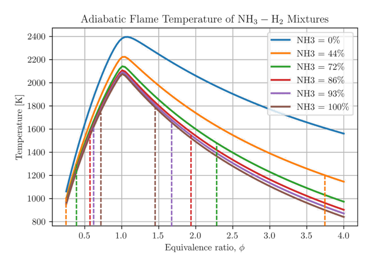
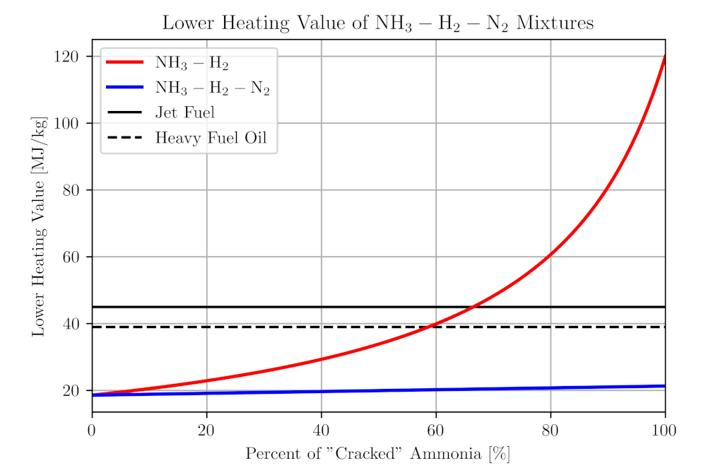
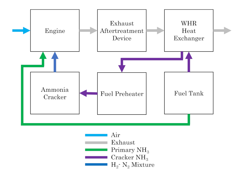
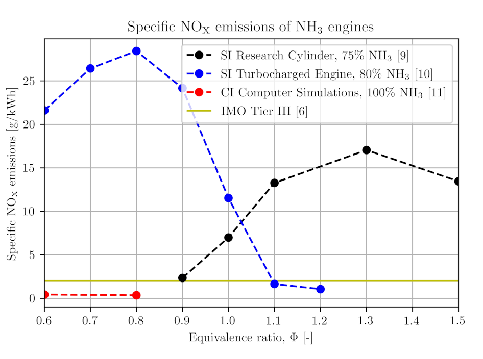
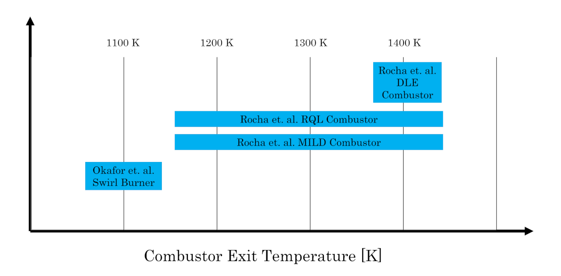
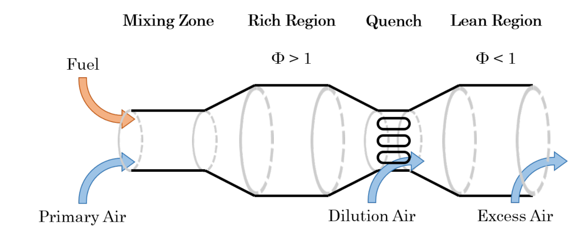
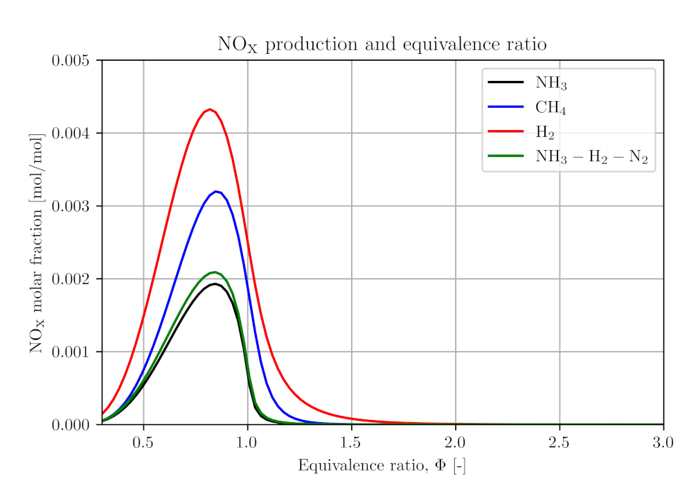
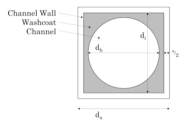
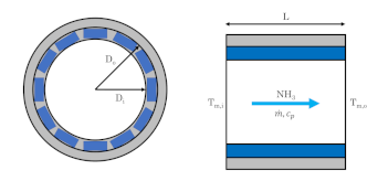
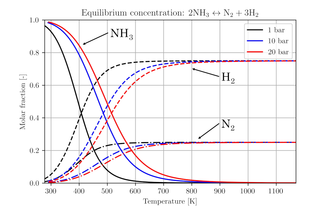
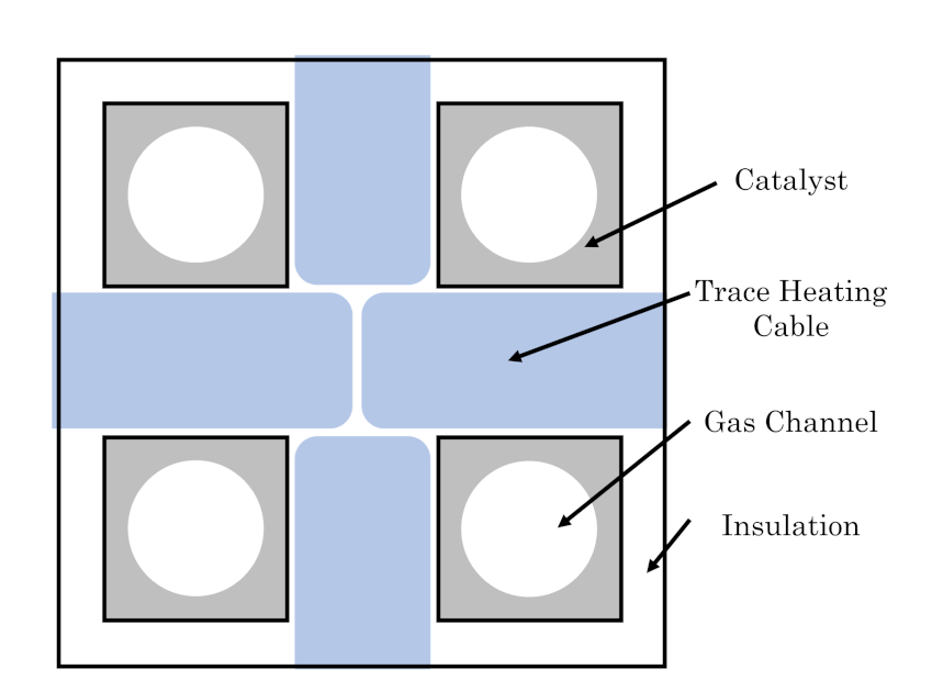
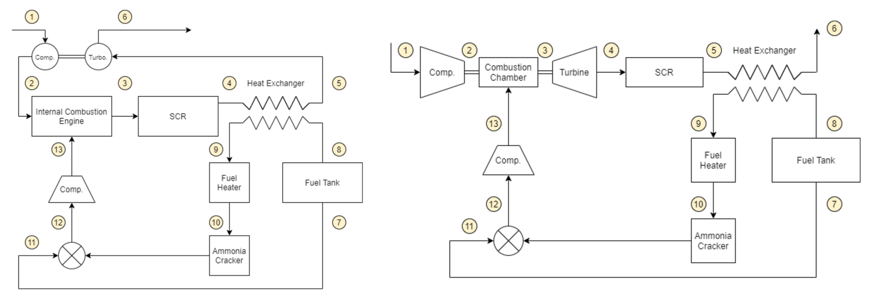
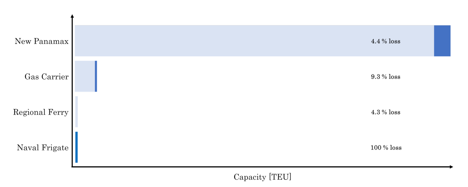
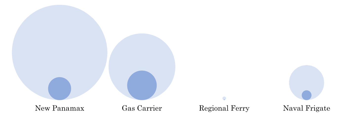
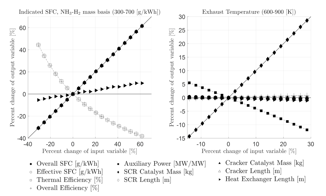
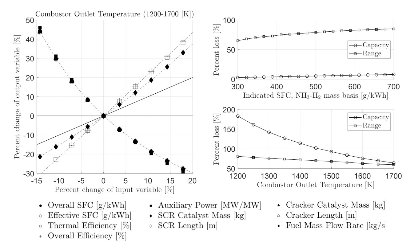
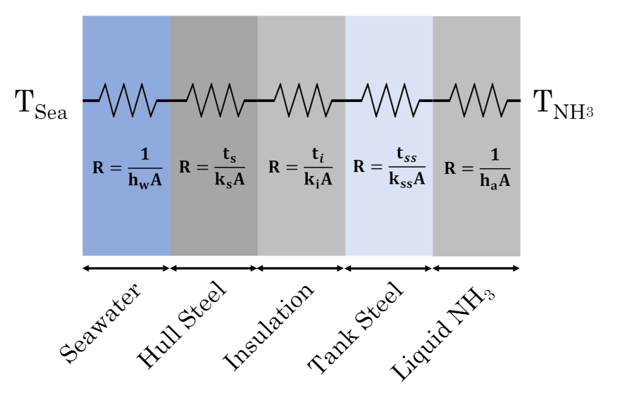
| Material | Thickness [mm] | Thermal Conductivity [W/m·K] |
|---|---|---|
| Mild steel hull | 16.5 | 45.0 |
| Glass wool insulation | — | 0.033 |
| Stainless steel tank | 6.0 | 14.0 |
Convection on the inside and outside of the tank is modelled as free convection. Free convection on vertical plates is modelled using the surface temperature, , the bulk temperature of the fluid, , and thermal properties of the fluid. The Rayleigh number, given below, and the Churchill and Chu correlation are used to generate a Nusselt number [38]. The length term associated with the Rayleigh number is the height of the plate. The Nusselt number is converted to a convection heat-transfer coefficient and is added to the resistor network in Figure A2.
Figure A2.
The thermal resistor network used to model the fuel tank.

The horizontal surfaces on the top and bottom of the tank use two correlations. The tank lid is modelled as the upper surface of a cold plate with respect to heat transfer from the air to the tank and as the bottom surface of a hot plate with respect to heat transfer from the tank to the liquid. Both cases fall under the correlation given below [38].
The bottom of the tank is modelled as the lower surface of a cold plate with respect to the seawater, and the upper surface of a hot plate with respect to the liquid ammonia. The Nusselt number is governed by the following correlation [38]:
The length term associated with the Rayleigh number for all flat plate cases is determined using the surface area of the plate and its perimeter [38].
References
- United Nations Framework Convention on Climate Change. The Paris Agreement. 2015. Available online: https://unfccc.int/process-and-meetings/the-paris-agreement/the-paris-agreement (accessed on 3 February 2021).
- Parliament of the United Kingdom. Climate Change Act 2008. 2008. Available online: https://www.legislation.gov.uk (accessed on 7 February 2021).
- International Energy Agency (IEA). International Shipping. 2020. Available online: https://www.iea.org/reports/international-shipping (accessed on 7 February 2021).
- International Energy Agency (IEA). IEA World. 2021. Available online: https://www.iea.org/world (accessed on 7 February 2021).
- International Transport Forum. Decarbonising Maritime Transport. Int. Transp. Forum Policy Pap. 2018, 47. [Google Scholar] [CrossRef]
- International Maritime Organization. Initial IMO Strategy on Reduction of GHG Emissions from Ships. 2018. Available online: https://wwwcdn.imo.org/localresources/en/OurWork/Environment/Documents/ (accessed on 20 February 2021).
- Hansson, J.; Brynolf, S.; Fridell, E.; Lehtveer, M. The Potential Role of Ammonia as Marine Fuel—Based on Energy Systems Modeling and Multi-Criteria Decision Analysis. Sustainability 2020, 12, 3265. [Google Scholar] [CrossRef] [Green Version]
- Singh, V.; Dincer, I.; Rosen, M.A. Chapter 4.2—Life Cycle Assessment of Ammonia Production Methods. In Exergetic, Energetic and Environmental Dimensions; Dincer, I., Colpan, C.O., Kizilkan, O., Eds.; Academic Press: Cambridge, MA, USA, 2018; pp. 935–959. [Google Scholar] [CrossRef]
- Mørch, C.; Bjerre, A.; Gøttrup, M.; Sorenson, S.; Schramm, J. Ammonia/hydrogen mixtures in an SI-engine: Engine performance and analysis of a proposed fuel system. Fuel 2011, 90, 854–864. [Google Scholar] [CrossRef]
- Lhuillier, C.; Brequigny, P.; Contino, F.; Mounaïm-Rousselle, C. Experimental study on ammonia/hydrogen/air combustion in spark ignition engine conditions. Fuel 2020, 269, 117448. [Google Scholar] [CrossRef]
- Lee, D.; Song, H. Development of combustion strategy for the internal combustion engine fueled by ammonia and its operating characteristics. J. Mech. Sci. Technol. 2018, 32, 1905–1925. [Google Scholar] [CrossRef]
- Verkamp, F.; Hardin, M.; Williams, J. Ammonia combustion properties and performance in gas-turbine burners. Symp. Int. Combust. 1967, 11, 985–992. [Google Scholar] [CrossRef]
- Valera-Medina, A.; Pugh, D.; Marsh, P.; Bulat, G.; Bowen, P. Preliminary study on lean premixed combustion of ammonia-hydrogen for swirling gas turbine combustors. Int. J. Hydrogen Energy 2017, 42, 24495–24503. [Google Scholar] [CrossRef]
- MAN Energy Solutions. Industry Consortium to Develop Medium-Speed, Ammonia-Fuelled Engine. 2021. Available online: https://www.man-es.com/company/press-releases/press-details/2021/04/07/industry-consortium-to-develop-medium-speed-ammonia-fuelled-engines (accessed on 8 July 2021).
- Wärtsilä Corporation. Wärtsilä Launches Major Test Programme towards Carbon-Free Solutions with Hydrogen and Ammonia. 2021. Available online: https://www.wartsila.com/media/news/14-07-2021-wartsila-launches-major-test-programme-towards-carbon-free-solutions-with-hydrogen-and-ammonia-2953362 (accessed on 16 July 2021).
- National Institute of Standards and Technology. NIST Chemistry WebBook. 2021. Available online: https://webbook.nist.gov/chemistry/ (accessed on 9 March 2021).
- Wijayanta, A.T.; Aziz, M. Ammonia Production from Algae via Integrated Hydrothermal Gasification, Chemical Looping, N2 Production, and NH3 Synthesis. Energy 2019, 174, 331–338. [Google Scholar] [CrossRef]
- Hasan, A.; Dincer, I. An ocean thermal energy conversion based system for district cooling, ammonia and power production. Int. J. Hydrogen Energy 2020, 45, 15878–15887. [Google Scholar] [CrossRef]
- Al-Aboosi, F.Y.; El-Halwagi, M.M.; Moore, M.; Nielsen, R.B. Renewable ammonia as an alternative fuel for the shipping industry. Curr. Opin. Chem. Eng. 2021, 31, 100670. [Google Scholar] [CrossRef]
- Shell. Military Jet Fuel Products. 2021. Available online: https://www.shell.com/business-customers/aviation/aviation-fuel/military-jet-fuel-grades.html (accessed on 9 March 2021).
- Stagni, A.; Cavallotti, C.; Arunthanayothin, S.; Song, Y.; Herbinet, O.; Battin-Leclerc, F.; Faravelli, T. An experimental, theoretical and kinetic-modeling study of the gas-phase oxidation of ammonia. React. Chem. Eng. 2020, 5, 696–711. [Google Scholar] [CrossRef] [Green Version]
- Pacific Northwest National Laboratory. Higher and Lower Heating Values. 2021. Available online: https://h2tools.org/hyarc/calculator-tools/lower-and-higher-heating-values-fuels (accessed on 9 March 2021).
- United Nations Conference on Trade and Development (UNCTAD). Merchant Fleet. 2020. Available online: https://stats.unctad.org/handbook/MaritimeTransport/MerchantFleet.html (accessed on 14 May 2021).
- MAN Energy Solutions. Propulsion Trends in Container Vessel Two-Stroke Engines. 2013. Available online: https://www.mandieselturbo.com (accessed on 10 March 2021).
- MAN Energy Solutions. 2020. Available online: https://man-es.com/applications/projectguides/2stroke/content/printed/G90ME-C10_5.pdf (accessed on 24 May 2021).
- Gaztransport Technigaz, 2021. Small and Mid-Scale LNG Ships. Available online: https://gtt.fr/applications/small-mid-scale (accessed on 2 June 2021).
- MAN Energy Solutions. MAN B&W G60ME-C9.5. 2020. Available online: https://man-es.com/applications/projectguides/2stroke/content/printed/G60ME-C9_5.pdf (accessed on 24 May 2021).
- J.F. Coldren. Cape May-Lewes Ferry History. 2014. Available online: https://www.cmlf.com/cape-may-lewes-ferry-history (accessed on 18 April 2021).
- Miller, W. A Ferry Tale: Crossing the Delaware on the Cape May-Lewes Ferry; Delapeake Publishing: Wilmington, DE, USA, 1984. [Google Scholar]
- MAN Energy Solutions. SEMT Pielstick PA6B STC; Technical report; MAN Energy Solutions: Augsburg, Germany, 2020. [Google Scholar]
- USNA Department of Naval Architecture and Ocean Engineering. Principles of Ship Performance; United States Naval Academy: Annapolis, MD, USA, 2021. [Google Scholar]
- General Electric Aviation. LM2500 Marine Gas Turbine. 2021. Available online: https://www.geaviation.com/sites/default/files/datasheet-lm2500.pdf (accessed on 28 March 2021).
- Brown, G.G.; Kline, J.E.; Rosenthal, R.E.; Washburn, A.R. Steaming on Convex Hulls. INFORMS J. Appl. Anal. 2007, 37, 342–352. [Google Scholar] [CrossRef] [Green Version]
- Karamitros, D.; Skarlis, S.A.; Koltsakis, G. Exhaust Gas Aftertreatment Technologies and Model Based Optimization. In Automotive Exhaust Emissions and Energy Recovery; Pesiridis, A., Ed.; Nova Science Publishers Incorporated: Hauppauge, NY, USA, 2014; Chapter 1b. [Google Scholar]
- Levenspiel, O. Chemical Reaction Engineering; John Wiley and Sons: New York, NY, USA, 1999. [Google Scholar]
- Alboshmina, N. Ammonia Cracking with Heat Transfer Improvement Technology. Ph.D. Thesis, Cardiff University, Cardiff, UK, 2019. [Google Scholar]
- Moran, M.; Shapiro, H.; Boettner, D.; Bailey, M. Fundamentals of Engineering Thermodynamics; John Wiley and Sons: New York, NY, USA, 2014. [Google Scholar]
- Incropera, F.; Dewitt, D.; Bergman, T.; Lavine, A. Introduction to Heat Transfer; John Wiley and Sons: New York, NY, USA, 2011. [Google Scholar]
- Treybal, R. Mass Transfer Operations; McGraw Hill Education: New York, NY, USA, 1968. [Google Scholar]
- Alturki, W. Four-Stroke and Two-Stroke Marine Engines Comparison and Application. Int. J. Eng. Res. Appl. 2017, 7, 49–56. [Google Scholar] [CrossRef]
- Mounaim-Rousselle, C.; Brequigny, P. Ammonia as Fuel for Low-Carbon Spark-Ignition Engines of Tomorrow’s Passenger Cars. Front. Mech. Eng. 2020, 6, 70. [Google Scholar] [CrossRef]
- Mashruk, S.; Xiao, H.; Valera-Medina, A. Rich-Quench-Lean model comparison for the clean use of humidified ammonia/hydrogen combustion systems. Int. J. Hydrogen Energy 2021, 46, 4472–4484. [Google Scholar] [CrossRef]
- Okafor, E.C.; Naito, Y.; Colson, S.; Ichikawa, A.; Kudo, T.; Hayakawa, A.; Kobayashi, H. Experimental and numerical study of the laminar burning velocity of CH4–NH3–air premixed flames. Combust. Flame 2018, 187, 185–198. [Google Scholar] [CrossRef]
- Tian, Z.; Li, Y.; Zhang, L.; Glarborg, P.; Qi, F. An experimental and kinetic modeling study of premixed NH3/CH4/O2/Ar flames at low pressure. Combust. Flame 2009, 156, 1413–1426. [Google Scholar] [CrossRef]
- Xiao, H.; Valera-Medina, A. Chemical kinetic mechanism study on premixed combustion of ammonia/hydrogen fuels for gas turbine use. J. Eng. Gas Turbines Power 2017, 139, 081504. [Google Scholar] [CrossRef]
- Glarborg, P.; Miller, J.A.; Ruscic, B.; Klippenstein, S.J. Modeling nitrogen chemistry in combustion. Prog. Energy Combust. Sci. 2018, 67, 31–68. [Google Scholar] [CrossRef] [Green Version]
- Otomo, J.; Koshi, M.; Mitsumori, T.; Iwasaki, H.; Yamada, K. Chemical kinetic modeling of ammonia oxidation with improved reaction mechanism for ammonia/air and ammonia/hydrogen/air combustion. Int. J. Hydrogen Energy 2018, 43, 3004–3014. [Google Scholar] [CrossRef]
- BMW Group. Petrol Engines in the BMW Group/ PSA Peugeot Citroen Cooperation. 2004. Available online: http://www.motoringfile.com/files/3_Technologietag_GB1102934639.pdf (accessed on 14 June 2021).
- Vedran, M.; Bozica, Z.; Jasna, P. Marine slow speed two-stroke diesel engine-Numerical analysis of efficiencies and important operating parameters. Mach. Technol. Mater. 2017, 10, 481–484. [Google Scholar]
- Nguyen-Schafer, H. Thermodynamics of Turbochargers. In Rotordynamics of Automotive Turbochargers; Springer: Berlin, Germany, 2012. [Google Scholar]
- Pounder, C.C. Pounder’s Marine Diesel Engines, 6th ed.; Butterworths: London, UK, 1984. [Google Scholar]
- Goodwin, D.G.; Speth, R.L.; Moffat, H.K.; Weber, B.W. Cantera: An Object-oriented Software Toolkit for Chemical Kinetics, Thermodynamics, and Transport Processes, Version 2.5.1. 2021. Available online: https://www.cantera.org (accessed on 3 February 2021). [CrossRef]
- Okafor, E.C.; Somarathne, K.K.A.; Hayakawa, A.; Kudo, T.; Kurata, O.; Iki, N.; Kobayashi, H. Towards the development of an efficient low-NOx ammonia combustor for a micro gas turbine. Proc. Combust. Inst. 2019, 37, 4597–4606. [Google Scholar] [CrossRef]
- Somarathne, K.D.K.A.; Hatakeyama, S.; Hayakawa, A.; Kobayashi, H. Numerical study of a low emission gas turbine like combustor for turbulent ammonia/air premixed swirl flames with a secondary air injection at high pressure. Int. J. Hydrogen Energy 2017, 42, 27388–27399. [Google Scholar] [CrossRef]
- Rocha, R.C.; Costa, M.; Bai, X.S. Combustion and Emission Characteristics of Ammonia under Conditions Relevant to Modern Gas Turbines. Combust. Sci. Technol. 2020, 193, 2514–2533. [Google Scholar] [CrossRef]
- Mattingly, J.D. Elements of Gas Turbine Propulsion; McGraw-Hill Inc.: Singapore, 1996. [Google Scholar]
- Smith, G.; Golden, D.; Frenklach, M.; Moriarty, N.; Eiteneer, B.; Goldenberg, M.; Bowman, C.; Hanson, R.; Song, S.; Gardiner, W.; et al. GRI-Mech 3.0. Available online: http://combustion.berkeley.edu/gri-mech/version30/text30.html (accessed on 3 February 2021).
- Schaub, G.; Unruh, D.; Wang, J.; Turek, T. Kinetic analysis of selective catalytic NOX reduction (SCR) in a catalytic filter. Chem. Eng. Process. Process. Intensif. 2003, 42, 365–371. [Google Scholar] [CrossRef]
- Nahavandi, M. Selective Catalytic Reduction of Nitric Oxide by Ammonia over V2O5/TiO2 in a Hollow Cylindrical Catalyst under Enhancing Effect of Electrohydrodynamics: A Kinetic Modeling Study. Ind. Eng. Chem. Res. 2014, 53, 12673–12688. [Google Scholar] [CrossRef]
- Kapas, N.; Shamim, T.; Laing, P. Effect of mass transfer on the performance of selective catalytic reduction (SCR) systems. J. Eng. Gas Turbines Power 2010, 133, 032801. [Google Scholar] [CrossRef]
- Russell, A.; Epling, W.S. Diesel Oxidation Catalysts. Catal. Rev. 2011, 53, 337–423. [Google Scholar] [CrossRef]
- Dahlin, S.; Englund, J.; Malm, H.; Feigel, M.; Westerberg, B.; Regali, F.; Skoglundh, M.; Pettersson, L.J. Effect of biofuel- and lube oil-originated sulfur and phosphorus on the performance of Cu-SSZ-13 and V2O5-WO3/TiO2 SCR catalysts. Special Contributions to Symposium F3 of XXVII IMRC-2018. Catal. Today 2021, 360, 326–339. [Google Scholar] [CrossRef]
- Dahlin, S.; Nilsson, M.; Bäckström, D.; Bergman, S.L.; Bengtsson, E.; Bernasek, S.L.; Pettersson, L.J. Multivariate analysis of the effect of biodiesel-derived contaminants on V2O5-WO3/TiO2 SCR catalysts. Appl. Catal. Environ. 2016, 183, 377–385. [Google Scholar] [CrossRef]
- qiang Tan, P.; chen Zhang, S.; yan Wang, S.; yuan Hu, Z.; Lou, D.M. Simulation on catalytic performance of fresh and aged SCR catalysts for diesel engines. J. Energy Inst. 2020, 93, 2280–2292. [Google Scholar] [CrossRef]
- Marberger, A.; Elsener, M.; Nuguid, R.J.G.; Ferri, D.; Kröcher, O. Thermal activation and aging of a V2O5/WO3-TiO2 catalyst for the selective catalytic reduction of NO with NH3. Appl. Catal. Gen. 2019, 573, 64–72. [Google Scholar] [CrossRef]
- Zhang, W.; Qi, S.; Pantaleo, G.; Liotta, L.F. WO3–V2O5 Active Oxides for NOx SCR by NH3: Preparation Methods, Catalysts’ Composition, and Deactivation Mechanism—A Review. Catalysts 2019, 9, 527. [Google Scholar] [CrossRef] [Green Version]
- Munson, B.; Okiishi, T.; Huebsch, W.; Rothmayer, A. Fundamentals of Fluids Mechanics; John Wiley and Sons: New York, NY, USA, 2013. [Google Scholar]
- Tang, M.J.; Cox, R.A.; Kalberer, M. Compilation and evaluation of gas phase diffusion coefficients of reactive trace gases in the atmosphere: Volume 1. Inorganic compounds. Atmos. Chem. Phys. 2014, 14, 9233–9247. [Google Scholar] [CrossRef] [Green Version]
- Pritchard, D.T.; Currie, J.A. Diffusion of coefficients of carbon dioxide, nitrous oxide, ethylene and ethane in air and their measurement. J. Soil Sci. 1982, 33, 175–184. [Google Scholar] [CrossRef]
- Specht, E. The Best Known Packings of Equal Circles in a Circle (Complete Up to N = 2600). 2018. Available online: http://hydra.nat.uni-magdeburg.de/packing/cci/ (accessed on 28 June 2021).
- Rolls-Royce. MT30 Marine Gas Turbine. 2021. Available online: https://www.rolls-royce.com/products-and-services/defence/naval/gas-turbines/mt30-marine-gas-turbine.aspx (accessed on 12 June 2021).
- Chromalox. Electrical Heat Tracing Systems Design Guide; Technical Report; Chromalox: Pittsburgh, PA, USA, 2019. [Google Scholar]
- Thorne and Derrick International. Thermon MIQ Mineral Insulated Heat Tracing Cables (Series Constant Wattage Heating Cable). Available online: https://www.heatingandprocess.com/product/product-category/thermon-miq-heat-tracing-cables/ (accessed on 2 July 2021).
- CED Engineering. Heat Tracing Systems; Technical Report; CED Engineering: Woodcliff Lake, NJ, USA, 2019. [Google Scholar]
- nVent Incorporated. Nuheat Weather-Ready Heat Trace Cable. Available online: https://assets.usesi.com/product-media/brochures/USESI_225591_brochure.pdf (accessed on 2 July 2021).
- Anderson, D. Preliminary Results from Screening Tests of Commercial Catalysts with Potential Use in Gas Turbine Combustors; Technical report; National Aeronautics and Space Administration (NASA): Cleveland, OH, USA, 1976. [Google Scholar]
- Chellappa, A.; Fischer, C.; Thomson, W. Ammonia decomposition kinetics over Ni-Pt/Al2O3 for PEM fuel cell applications. Appl. Catal. Gen. 2002, 227, 231–240. [Google Scholar] [CrossRef]
- Miana, M.; Legorburo, R.; Díez, D.; Hwang, Y.H. Calculation of Boil-Off Rate of Liquefied Natural Gas in Mark III tanks of ship carriers by numerical analysis. Appl. Therm. Eng. 2016, 93, 279–296. [Google Scholar] [CrossRef]
- Dimopoulos, G.; Frangopoulos, C. A Dynamic Model for Liquefied Natural Gas Evaporation During Marine Transportation. Int. J. Thermodyn. 2008, 11, 123–131. [Google Scholar] [CrossRef]
- Maran Gas. Boil-Off Characteristics of Maran Gas Amphipolis; Technical report; Maran Gas Maritime Incorporated: Athens, Greece, 2016. [Google Scholar]
- Dincer, I. 1.7 Energy and Exergy Efficiencies. In Comprehensive Energy Systems; Dincer, I., Ed.; Elsevier: Oxford, UK, 2018; pp. 265–339. [Google Scholar] [CrossRef]
- Heywood, J. Internal Combustion Engine Fundamentals; McGraw Hill: New York, NY, USA, 1988. [Google Scholar]
- 16-Acoustic and Thermal Insulating Materials. Building Decorative Materials; Li, Y., Ren, S., Eds.; Woodhead Publishing: Sawston, UK, 2011; pp. 359–374. [Google Scholar] [CrossRef]
Figure 1.
The adiabatic flame temperature of NH3-H2 mixtures as a function of equivalence ratio and the associated flame stability limits [12,13]. The simulations use the Stagni et al. [21] combustion mechanism.

Figure 2.
The lower heating values (LHVs) of NH3-H2 and NH3-H2-N2 mixtures as a function of the percent of cracked ammonia [16,22].

Figure 3.
The layout of the proposed ammonia powertrain.

Figure 4.
The specific emissions of various NH3-H2 engines as a function of equivalence ratio [6,9,10,11].

Figure 5.
The combustor exhaust temperature ranges from various studies modelling the combustion of pure ammonia in a GT burner [53,54,55]. For the current study, 1400 K was ultimately selected as the combustor exhaust temperature.

Figure 6.
A diagram of a rich-quench-lean (RQL) burner. Fuel and primary air mix prior to entering the rich region. is not formed in the rich region due to chemical phenomena. The exhaust gases from the rich region are quenched to yield a lean mixture for the final stage of the combustor. The quenching air lowers the temperature of the combustion gases to limit the formation of thermal . The flow of combustion gases through the burner is continuous.

Figure 7.
The molar fraction at various equivalence ratios for pure methane, ammonia, and hydrogen, each burning in dry air. The results represent chemical equilibrium in a well-stirred reactor. Methane combustion is modelled using the GRI-Mech 3.0 mechanism [57]. Ammonia and hydrogen combustion is modelled using the Stagni et al. [21] combustion mechanism.

Figure 8.
A single channel is the selective catalytic reduction (SCR) device with the outer channel diameter, inner channel diameter, circular diameter, and wall thickness labelled.
Figure 8.
A single channel is the selective catalytic reduction (SCR) device with the outer channel diameter, inner channel diameter, circular diameter, and wall thickness labelled.

Figure 9.
A diagram of a counterflow shell and tube heat exchanger (HX).

Figure 10.
The cross-sections of one fuel heating tube. The head-on view (left) shows a notional arrangement of heat tracing cables around the outer surface of the tube. The side-view (right) shows the mean inlet and outlet temperatures. Heat trace cables are denoted in blue, insulation in grey, and the fuel in white. Not to scale.

Figure 11.
The equilibrium molar fractions of ammonia and its constituents as a function of temperature. Produced using the Stagni et al. [21] combustion mechanism.
Figure 11.
The equilibrium molar fractions of ammonia and its constituents as a function of temperature. Produced using the Stagni et al. [21] combustion mechanism.

Figure 12.
A notional cross-section of the catalytic ammonia cracker proposed in Section 2.8 with cell walls thick enough to accommodate electrical trace heaters.
Figure 12.
A notional cross-section of the catalytic ammonia cracker proposed in Section 2.8 with cell walls thick enough to accommodate electrical trace heaters.

Figure 13.
The process flow diagrams of an ammonia-fuelled ICE powertrain (left) and GT powertrain (right).
Figure 13.
The process flow diagrams of an ammonia-fuelled ICE powertrain (left) and GT powertrain (right).

Figure 14.
The cargo carrying capacity of the vessels considered in this study and the associated absolute and relative loss of cargo carrying capacity compared to conventional vessels.
Figure 14.
The cargo carrying capacity of the vessels considered in this study and the associated absolute and relative loss of cargo carrying capacity compared to conventional vessels.

Figure 15.
A scale comparison of the original and adjusted range of the vessels after adopting ammonia-fuelled powertrains.
Figure 15.
A scale comparison of the original and adjusted range of the vessels after adopting ammonia-fuelled powertrains.

Figure 16.
The relative change in relevant output values with respect to the relative change of one input value, in this case, the input indicated SFC on an NH3-H2 mass basis (left) and the ICE exhaust temperature (right). A horizontal line represents the case that changing the input has no impact on the output variable. A line with a slope of 1.0 represents direct proportionality between changes to the input and changes to the output.

Figure 17.
(left) The relative change in relevant output values with respect to the relative change of one input value, in this case, the GT combustor exit temperature. (right) A comparison of how changes to ICE input indicated SFC and GT combustor exit temperature impact the loss of range and capacity of an ICE-powered New Panamax vessel (top) and a GT-powered naval frigate (bottom).

Table 1.
The combustion properties of JP-4, ammonia, and hydrogen, adapted from [12]. The minimum quenching distance and minimum ignition energy are determined experimentally at 1 atm. The laminar burning velocity is determined experimentally at 422 K (300° F) and 1 atm. The heat of vaporisation is a referenced value, and the flame stability limits are generalised from the gas turbine (GT) burner. JP-4 is no longer manufactured, but its properties are very similar to modern jet fuel [20].
| Property | Units | JP-4 | Ammonia | Hydrogen |
|---|---|---|---|---|
| Min. quenching distance | cm | 0.203 | 0.699 | 0.0635 |
| Min. ignition energy | mJ | 0.3 | 9.0 | 0.2 |
| Laminar burning velocity | cm/s | 62.2 | 15.0 | 351 |
| Heat of vaporisation | kJ/kg | 361 | 1180 | 449 |
| Flammability limits | range | 0.55–4.24 | 0.724–1.46 | 0.182–8.84 |
Table 2.
The physical characteristics, engine requirements, capacity, and range of each of the four classifications of vessel discussed in the present study [24,25,26,27,28,29,30,31,32] .
| Quantity | Units | New Panamax | Gas Carrier | Regional Ferry | Naval Frigate |
|---|---|---|---|---|---|
| Design draft | m | 14.5 | 7.4 | 2.1 | 9.1 |
| Overall length | m | 368.0 | 176.0 | 98.0 | 153.6 |
| Maximum breadth | m | 51.0 | 28.8 | 21.0 | 20.3 |
| Displacement | tonnes | 154,200 | 37,400 | 2000 | 7595 |
| Cargo capacity | TEU | 14,000 | 831 | 90 | 81 |
| MCR speed | knots | 25 | 17.5 | 15.5 | 20 |
| Maximum range | nmi | 12,000 | 8400 | 446 | 4400 |
| MCR engine power | MW | 78 | 13.4 | 6.48 | 88 |
Table 3.
The input parameters for the internal combustion (ICE) model based on data from Lhuillier et al. [10]. The primary input variable is the desired effective power, but all parameters can be changed to reflect new experimental data. * The effective power should match the power requirements from Section 2.3. † Indicated specific fuel consumption (SFC) values are the published values prior to mass correction due to nitrogen dilution. The code corrects these values itself.
| Input Parameter | Units | Value |
|---|---|---|
| Effective power | MW | * |
| Mechanical efficiency | — | 92.85% |
| Exhaust temperature | K | 720 |
| Equivalence ratio | — | 0.7 |
| Indicated SFC † | g/kWh | 430/533.2 |
| at exhaust | ppm | 5000 |
| NH3 at exhaust | ppm | 5000 |
| Ammonia/hydrogen ratio | — | 4:1 |
Table 4.
The input parameters for the GT engine model based on the literature values [53,54,55]. The desired fuel flow rate is the primary variable, but all values can be changed to reflect new experimental data. * The fuel flow rate is altered until the effective power output is equal to the required power as defined by Section 2.3.
| Input Parameter | Units | Value |
|---|---|---|
| Fuel flow rate | kg/s | * |
| Compression ratio | — | 18 |
| Mechanical efficiency | — | 99.0% |
| Combustor exit temperature | K | 1400 |
| Global equivalence ratio | — | 0.4 |
| — | 89% | |
| — | 89% | |
| — | 89% | |
| Combustor pressure loss | — | 5.0% |
| at exhaust | ppm | 820 |
| NH3 at exhaust | ppm | 5.2 |
| Ammonia/hydrogen ratio | — | 4:1 |
Table 5.
The fixed characteristics of marine SCR devices considered in this analysis. The washcoat loading and washcoat density values are similar to those used in automotive SCRs [34,35].
| Quantity | Units | Value |
|---|---|---|
| Active catalyst | — | |
| CPSM | cells/ | 465,000 |
| Wall thickness | mm | 0.15 |
| Washcoat loading | 120 | |
| Washcoat density | g/ | 1500 |
Table 6.
Shell and tube diameters for the waste heat recovery (WHR) device based on effective output power [25,27,30,32,70,71].
| Power [MW] | Engine | Shell Diameter [m] | Tube Diameter [m] |
|---|---|---|---|
| 78 | ICE | 2.0 | 0.05315 |
| 13.4 | ICE | 1.0 | 0.02657 |
| 6.48 | ICE | 0.5 | 0.01329 |
| 22 | GT | 2.0 | 0.05315 |
Table 7.
The generic characteristics of a series-connected, mineral-insulated, flat cross-section heat trace cable [74,75].
| Quantity | Units | Value |
|---|---|---|
| Width | m | 0.0131 |
| Thickness | m | 0.0056 |
| Power | W/m | 262.5 |
| Maximum temperature | K | 1088 |
Table 8.
The fixed characteristics of the marine ammonia cracking devices considered in this study.
| Quantity | Units | Value |
|---|---|---|
| Active catalyst | — | G43 (Ni-Pt) |
| CPSM | cells/ | 6200 |
| Wall thickness | mm | 5.75 |
| Washcoat loading | 1130 | |
| Washcoat density | g/ | 3950 |
Table 9.
The state points corresponding to the process flow diagram given by Figure 13 for an ICE 78 MW New Panamax vessel at maximum continuous rating (MCR).
Table 9.
The state points corresponding to the process flow diagram given by Figure 13 for an ICE 78 MW New Panamax vessel at maximum continuous rating (MCR).
| Quantity | Units | 1 | 2 | 3 | 4 | 5 | 6 | 7 | 8 | 9 | 10 | 11 | 12 | 13 |
|---|---|---|---|---|---|---|---|---|---|---|---|---|---|---|
| Temperature | K | 288.2 | 309.2 | 720.0 | 782.6 | 772.0 | 757.1 | 298.0 | 298.0 | 686.7 | 900.0 | 900.0 | 423.9 | 451.1 |
| Pressure | bar | 1.01 | 1.20 | 1.24 | 1.14 | 1.14 | 1.01 | 1.01 | 1.01 | 1.01 | 1.01 | 1.01 | 1.01 | 1.30 |
| Mass flow | kg/s | 98.7 | 98.7 | 110.1 | 110.1 | 110.1 | 110.1 | 9.8 | 1.6 | 1.6 | 1.6 | 1.6 | 11.4 | 11.4 |
| Molar flow | mol/s | 3406 | 3406 | 4235 | 4240 | 4240 | 4240 | 572 | 95 | 95 | 95 | 190 | 763 | 763 |
| O2 | mol. frac. | 0.21 | 0.21 | 0.05 | 0.05 | 0.05 | 0.05 | — | — | — | — | — | — | — |
| N2 | mol. frac. | 0.78 | 0.78 | 0.7 | 0.7 | 0.7 | 0.7 | — | — | — | — | 0.25 | 0.06 | 0.06 |
| mol. frac. | — | — | 0.01 | — | — | — | — | — | — | — | — | — | — | |
| NH3 | mol. frac. | — | — | 0.01 | — | — | — | 1.00 | 1.00 | 1.00 | 1.00 | — | 0.75 | 0.75 |
| H2 | mol. frac. | — | — | — | — | — | — | — | — | — | — | 0.75 | 0.19 | 0.19 |
| H2O | mol. frac. | — | — | 0.23 | 0.24 | 0.24 | 0.24 | — | — | — | — | — | — | — |
Table 10.
The state points corresponding to the process flow diagram given by Figure 13 for an ICE 13.4 MW gas carrier at MCR.
Table 10.
The state points corresponding to the process flow diagram given by Figure 13 for an ICE 13.4 MW gas carrier at MCR.
| Quantity | Units | 1 | 2 | 3 | 4 | 5 | 6 | 7 | 8 | 9 | 10 | 11 | 12 | 13 |
|---|---|---|---|---|---|---|---|---|---|---|---|---|---|---|
| Temperature | K | 288.2 | 309.2 | 720.0 | 782.6 | 771.6 | 756.7 | 298.0 | 298.0 | 685.8 | 900.0 | 900.0 | 423.9 | 451.1 |
| Pressure | bar | 1.01 | 1.20 | 1.18 | 1.14 | 1.14 | 1.01 | 1.01 | 1.01 | 1.01 | 1.01 | 1.01 | 1.01 | 1.30 |
| Mass flow | kg/s | 17.0 | 17.0 | 18.9 | 18.9 | 18.9 | 18.9 | 1.7 | 0.3 | 0.3 | 0.3 | 0.3 | 2.0 | 2.0 |
| Molar flow | mol/s | 585 | 585 | 727 | 728 | 728 | 728 | 98 | 16 | 16 | 16 | 33 | 131 | 131 |
| O2 | mol. frac. | 0.21 | 0.21 | 0.05 | 0.05 | 0.05 | 0.05 | — | — | — | — | — | — | — |
| N2 | mol. frac. | 0.78 | 0.78 | 0.7 | 0.7 | 0.7 | 0.7 | — | — | — | — | 0.25 | 0.06 | 0.06 |
| mol. frac. | — | — | 0.01 | — | — | — | — | — | — | — | — | — | — | |
| NH3 | mol. frac. | — | — | 0.01 | — | — | — | 1.00 | 1.00 | 1.00 | 1.00 | — | 0.75 | 0.75 |
| H2 | mol. frac. | — | — | — | — | — | — | — | — | — | — | 0.75 | 0.19 | 0.19 |
| H2O | mol. frac. | — | — | 0.23 | 0.24 | 0.24 | 0.24 | — | — | — | — | — | — | — |
Table 11.
The state points corresponding to the process flow diagram given by Figure 13 for an ICE 6.48 MW regional ferry at MCR.
Table 11.
The state points corresponding to the process flow diagram given by Figure 13 for an ICE 6.48 MW regional ferry at MCR.
| Quantity | Units | 1 | 2 | 3 | 4 | 5 | 6 | 7 | 8 | 9 | 10 | 11 | 12 | 13 |
|---|---|---|---|---|---|---|---|---|---|---|---|---|---|---|
| Temperature | K | 288.2 | 309.2 | 720.0 | 782.6 | 771.6 | 756.6 | 298.0 | 298.0 | 689.3 | 900.0 | 900.0 | 423.9 | 451.1 |
| Pressure | bar | 1.01 | 1.20 | 1.41 | 1.14 | 1.14 | 1.01 | 1.01 | 1.01 | 1.01 | 1.01 | 1.01 | 1.01 | 1.30 |
| Mass flow | kg/s | 10.2 | 10.2 | 11.3 | 11.3 | 11.3 | 11.3 | 1.0 | 0.2 | 0.2 | 0.2 | 0.2 | 1.2 | 1.2 |
| Molar flow | mol/s | 351 | 351 | 436 | 437 | 437 | 437 | 59 | 10 | 10 | 10 | 20 | 79 | 79 |
| O2 | mol. frac. | 0.21 | 0.21 | 0.05 | 0.05 | 0.05 | 0.05 | — | — | — | — | — | — | — |
| N2 | mol. frac. | 0.78 | 0.78 | 0.7 | 0.7 | 0.7 | 0.7 | — | — | — | — | 0.25 | 0.06 | 0.06 |
| mol. frac. | — | — | 0.01 | — | — | — | — | — | — | — | — | — | — | |
| NH3 | mol. frac. | — | — | 0.01 | — | — | — | 1.00 | 1.00 | 1.00 | 1.00 | — | 0.75 | 0.75 |
| H2 | mol. frac. | — | — | — | — | — | — | — | — | — | — | 0.75 | 0.19 | 0.19 |
| H2O | mol. frac. | — | — | 0.23 | 0.24 | 0.24 | 0.24 | — | — | — | — | — | — | — |
Table 12.
The state points corresponding to the process flow diagram given by Figure 13 for a single 22 MW GT used by a naval frigate running in trail shaft mode. The naval frigate is equipped with 4 GTs, but these data describe the performance of a single GT at MCR.
Table 12.
The state points corresponding to the process flow diagram given by Figure 13 for a single 22 MW GT used by a naval frigate running in trail shaft mode. The naval frigate is equipped with 4 GTs, but these data describe the performance of a single GT at MCR.
| Quantity | Units | 1 | 2 | 3 | 4 | 5 | 6 | 7 | 8 | 9 | 10 | 11 | 12 | 13 |
|---|---|---|---|---|---|---|---|---|---|---|---|---|---|---|
| Temperature | K | 288.2 | 691.2 | 1400.0 | 778.1 | 788.6 | 784.1 | 298.0 | 298.0 | 593.0 | 900.0 | 900.0 | 423.9 | 817.5 |
| Pressure | bar | 1.01 | 18.24 | 17.33 | 1.04 | 1.01 | 1.01 | 1.01 | 1.01 | 1.01 | 1.01 | 1.01 | 1.01 | 20.00 |
| Mass flow | kg/s | 55.3 | 55.3 | 58.8 | 58.8 | 58.8 | 58.8 | 2.9 | 0.5 | 0.5 | 0.5 | 0.5 | 3.4 | 3.4 |
| Molar flow | mol/s | 1911 | 1911 | 2163 | 2164 | 2166 | 2166 | 172 | 29 | 29 | 29 | 58 | 230 | 230 |
| O2 | mol. frac. | 0.21 | 0.21 | 0.11 | 0.11 | 0.11 | 0.11 | — | — | — | — | — | — | — |
| N2 | mol. frac. | 0.78 | 0.78 | 0.73 | 0.73 | 0.73 | 0.73 | — | — | — | — | 0.25 | 0.06 | 0.06 |
| mol. frac. | — | — | 0.001 | 0.0004 | — | — | — | — | — | — | — | — | — | |
| NH3 | mol. frac. | — | — | — | 0.0004 | — | — | 1.00 | 1.00 | 1.00 | 1.00 | — | 0.75 | 0.75 |
| H2 | mol. frac. | — | — | — | — | — | — | — | — | — | — | 0.75 | 0.19 | 0.19 |
| H2O | mol. frac. | — | — | 0.15 | 0.15 | 0.15 | 0.15 | — | — | — | — | — | — | — |
Table 13.
A comparison of the average performance of ammonia-fuelled ICEs and GTs per effective output power.
Table 13.
A comparison of the average performance of ammonia-fuelled ICEs and GTs per effective output power.
| Quantity | Units | ICE | GT |
|---|---|---|---|
| Thermal efficiency | % | 36.2 | 34.2 |
| Overall efficiency | % | 33.5 | 27.1 |
| Effective SFC | g/kWh | 524.8 | 559.9 |
| Overall SFC | g/kWh | 566.4 | 700.4 |
| Exhaust mass flow per output effective power | kg/s·MW | 1.5 | 2.7 |
| Additional power input per output effective power | MW/MW | 0.08 | 0.25 |
| Mass of catalyst per output effective power | /MW | 2.8 | 6.3 |
| Mass of G43 catalyst per output effective power | /MW | 22.0 | 23.4 |
Publisher’s Note: MDPI stays neutral with regard to jurisdictional claims in published maps and institutional affiliations. |
© 2021 by the authors. Licensee MDPI, Basel, Switzerland. This article is an open access article distributed under the terms and conditions of the Creative Commons Attribution (CC BY) license (https://creativecommons.org/licenses/by/4.0/).
Share and Cite
MDPI and ACS Style
Imhoff, T.B.; Gkantonas, S.; Mastorakos, E. Analysing the Performance of Ammonia Powertrains in the Marine Environment. Energies 2021, 14, 7447. https://0-doi-org.brum.beds.ac.uk/10.3390/en14217447
AMA Style
Imhoff TB, Gkantonas S, Mastorakos E. Analysing the Performance of Ammonia Powertrains in the Marine Environment. Energies. 2021; 14(21):7447. https://0-doi-org.brum.beds.ac.uk/10.3390/en14217447
Chicago/Turabian StyleImhoff, Thomas Buckley, Savvas Gkantonas, and Epaminondas Mastorakos. 2021. "Analysing the Performance of Ammonia Powertrains in the Marine Environment" Energies 14, no. 21: 7447. https://0-doi-org.brum.beds.ac.uk/10.3390/en14217447
Note that from the first issue of 2016, this journal uses article numbers instead of page numbers. See further details here.