Article

Study on Convective Heat Transfer of Supercritical Nitrogen in a Vertical Tube for Liquid Air Energy Storage

1
Hubei Key Laboratory of Advanced Technology for Automotive Components, School of Automotive Engineering, Wuhan University of Technology, Wuhan 430070, China
2
Birmingham Centre for Energy Storage, School of Chemical Engineering, University of Birmingham, Birmingham B15 2TT, UK
*
Authors to whom correspondence should be addressed.
Submission received: 24 October 2021 / Revised: 11 November 2021 / Accepted: 17 November 2021 / Published: 19 November 2021
(This article belongs to the Special Issue Advanced Energy Storage for Green Buildings)

Abstract

:
The convective heat transfer behavior of supercritical nitrogen (S-N2) has played a significant role in optimizing the design of recently emerging cryogenic cold storage and recovery systems. However, studies on S-N2 heat transfer have been relatively scarce, not to mention that there is a legitimate urge for a robust numerical model to accurately predict and explain S-N2 heat transfer under various working conditions. In this paper, both experimental and numerical studies were conducted for convective heat transfer of S-N2 in a small vertical tube. The results demonstrated that the standard k-ε model performed better for predicting the key heat transfer characteristics of S-N2 than the SST k-ω model. The effects of heat flux and inlet pressure on the heat transfer characteristics under a large mass flux were evaluated. The variation mechanisms of local heat transfer performance were revealed by illustrating radial profiles of thermophysical properties and turbulent parameters of N2. It was found that the local performance variation along the flow direction was mainly determined by the radial profile of specific heat while the variation of the best local performance with the ratio of heat flux to mass flux was mainly determined by the radial profile of turbulent viscosity.

1. Introduction

Supercritical nitrogen (S-N2) has attracted increasing attention in multiple applications during recent years. For example, liquid N2/air serves as a dual working medium for both electricity storage and heat transfer in the blossoming liquid air energy storage (LAES) technology, which has several advantages including high energy storage density, no geographical constraints, no environment pollution, and long service life [1,2]. During the energy discharging process for producing electricity, liquid N2/air is first pressurized to more than the critical pressure and then heated from a subcritical to supercritical condition. It has been demonstrated that the heat transfer performance of S-N2 or supercritical air is crucial to the round-trip efficiency of the LAES system [3]. The compression heat can be stored by heat transfer between S-N2 with a thermal energy storage unit [4] and then used to heat liquid N2 during the discharging process. Furthermore, S-N2 or supercritical air at high temperatures can be employed to heat liquefied natural gas (LNG) by replacing the conventionally used seawater for recovering the cold energy during the LNG regasification, which is usually wasted. It has been shown that the chilled supercritical air or S-N2 can significantly reduce the power consumption of air liquefaction or LAES [5,6]. Besides, S-N2 also plays important roles in high-temperature superconducting and polymer processing, where it serves as a coolant [7] and a blowing agent [8], respectively. As shown in the above-mentioned applications, the heat transfer performance of S-N2 is of vital importance.
As with other supercritical fluids, the thermodynamic properties of S-N2 notably vary with temperature at a constant pressure beyond the critical pressure, as shown in Figure 1. The critical pressure of N2 is p c = 3.4 MPa while its critical temperature is T c = 126.2 K. As Figure 1 shows, there exists a maximum value of specific heat for each pressure over p c and the corresponding temperature is called the “pseudo-critical” temperature T p c , which is more than T c ( T p c = 128.2 K at p = 3.8 MPa and T p c = 142.7 K at p = 7 MPa). The thermophysical properties of N2, such as specific heat, density, viscosity, and thermal conductivity change most dramatically near T p c at p = 3.8 MPa, while they vary relatively gently at p = 7 MPa.
As a result of the extreme variation of thermophysical properties, it is very challenging to comprehensively understand the complicated heat transfer characteristics of S-N2. Over the past few decades, a considerable amount of efforts have been made to investigate the heat transfer behaviors of different supercritical fluids [10]. Wang et al. [11] performed numerical simulations to explore heat transfer characteristics of supercritical water flowing upward in a circular tube with a semi-circular heating condition based on an improved turbulence model. They stated that heat transfer degradation might be mitigated via properly tuning the heating condition of the semi-circular profile. Chen et al. [12] experimentally analyzed the heat transfer performance of supercritical water in a three-rod bundle and established a new correlation of heat transfer coefficient with errors of less than ±15%. Zhang et al. [13] experimentally examined the heat transfer deterioration behaviors of supercritical carbon dioxide (S-CO2). They found that it was easy to detect the heat transfer deterioration when the mass flux was larger than 120 kg/(m2·s), which could be attributed to flow re-laminarization due to the sharply varied S-CO2 properties. The position where the deterioration occurred was found to move towards the inlet as the mass flux increased. Ren et al. [14] numerically explored the impacts of thermophysical property variations and buoyancy force on the local heat transfer behaviors of S-CO2 in a cooled horizontal semi-circular channel inside a printed circuit heat exchanger. Lei et al. [15] asserted that the S-CO2 heat transfer was substantially affected by buoyancy, especially under high heat fluxes and low mass fluxes through an experimental investigation of S-CO2 flowing in a vertical tube of 5 mm in diameter. Wang et al. [16] used the AKN k-ε turbulence model to examine the S-CO2 heat transfer in cooled tubes with 20 mm diameter under various inclined angles. Tian et al. [17] also adopted the AKN k-ε turbulence model to investigate the convective heat transfer of supercritical R134a flowing in a horizontal tube under different tube diameters with considering the effects of property variations and buoyancy.
In addition to the above research on supercritical fluids including water and CO2, several studies have been published focusing on the S-N2 heat transfer. Yu et al. [18] evaluated and optimized the performance of S-N2 based heat exchanger used for LAES based on the energy balance principle and exergy dissipation theory. Dimitrov et al. [19] reported preliminary experimental results concerning the S-N2 heat transfer in a large vertical tube of 20 mm in diameter under extremely small mass and heat fluxes. Negoescu et al. [20] adopted the k-ε model to explore S-N2 heat transfer in a vertical tube with a diameter of 2 mm for a variety of working conditions in mass and heat fluxes. Zhang et al. [21] conducted experiments on S-N2 heat transfer in a vertically upward tube of 2 mm in diameter as well as corresponding numerical analysis based on the shear stress transfer (SST) k-ω model and axisymmetric assumption. Their results indicated that the simulated wall temperature had a good agreement with the experimental results at small ratios of heat flux to mass flux whereas there were significant differences at large ratios. Furthermore, the comparison in heat transfer coefficient between numerical and experimental results indicated that the numerical results could not perfectly reproduce the characteristics of N2 heat transfer near T p c . Zhu et al. [22] also adopted the SSG Reynolds stress model to explore the impacts of main system parameters on the heat transfer characteristics of S-N2 flowing vertically downward in a 2-mm-diameter tube with discussing the relationship between the boundary layer and heat transfer enhancement. They used the experimental results (i.e., wall temperatures) of Zhang et al. [21] to validate their numerical model, but the consistency at large ratios of heat flux to mass flux ( q / G = 155 J/kg) is not as good as that at small ratios. Wang et al. [23] conducted experimental investigation on the role of a hiTRANTM wire matrix tube insert in improving the heat transfer performance of upward S-N2 flow in a small vertical tube. Their results verified more than 42% performance improvement because of the intensified overall fluid mixing resulted from the wire matrix insert.
Overall, studies concerning the S-N2 heat transfer are relatively scarce compared to other supercritical fluids (e.g., water and CO2). Furthermore, the previously published numerical works about S-N2 have not completely solved the puzzle of which turbulence model could more precisely predict the heat transfer characteristics near T p c , especially for large ratios of heat flux to mass flux. Moreover, the mechanism of heat transfer performance variation of S-N2 caused by varying thermophysical properties of N2 has not been revealed to date. To optimize S-N2 heat transfer systems, studies about the S-N2 heat transfer behaviors under a wider range of working conditions in mass flux, heat flux and pressure are also undoubtedly required. Therefore, in this study, both experimental and numerical studies were conducted, and results were compared to seek a more suitable turbulence model for predicting the S-N2 heat transfer characteristics in a heated vertical circular mini-tube. The effects of the ratio of heat flux to mass flux and pressure on the S-N2 heat transfer performance at large mass fluxes were discussed in detail. Special attention was paid to the comparisons of N2 thermophysical properties and turbulence parameters along the radial direction among different axial positions and between the cases with different ratios of heat flux to mass flux, to explain the variation mechanism of heat transfer performance along the axial direction and with the ratio of heat flux to mass flux. This work provides an important reference for understanding the variation mechanism of S-N2 heat transfer performance and a prelude for elevating the heat transfer efficiency in S-N2 based energy systems.

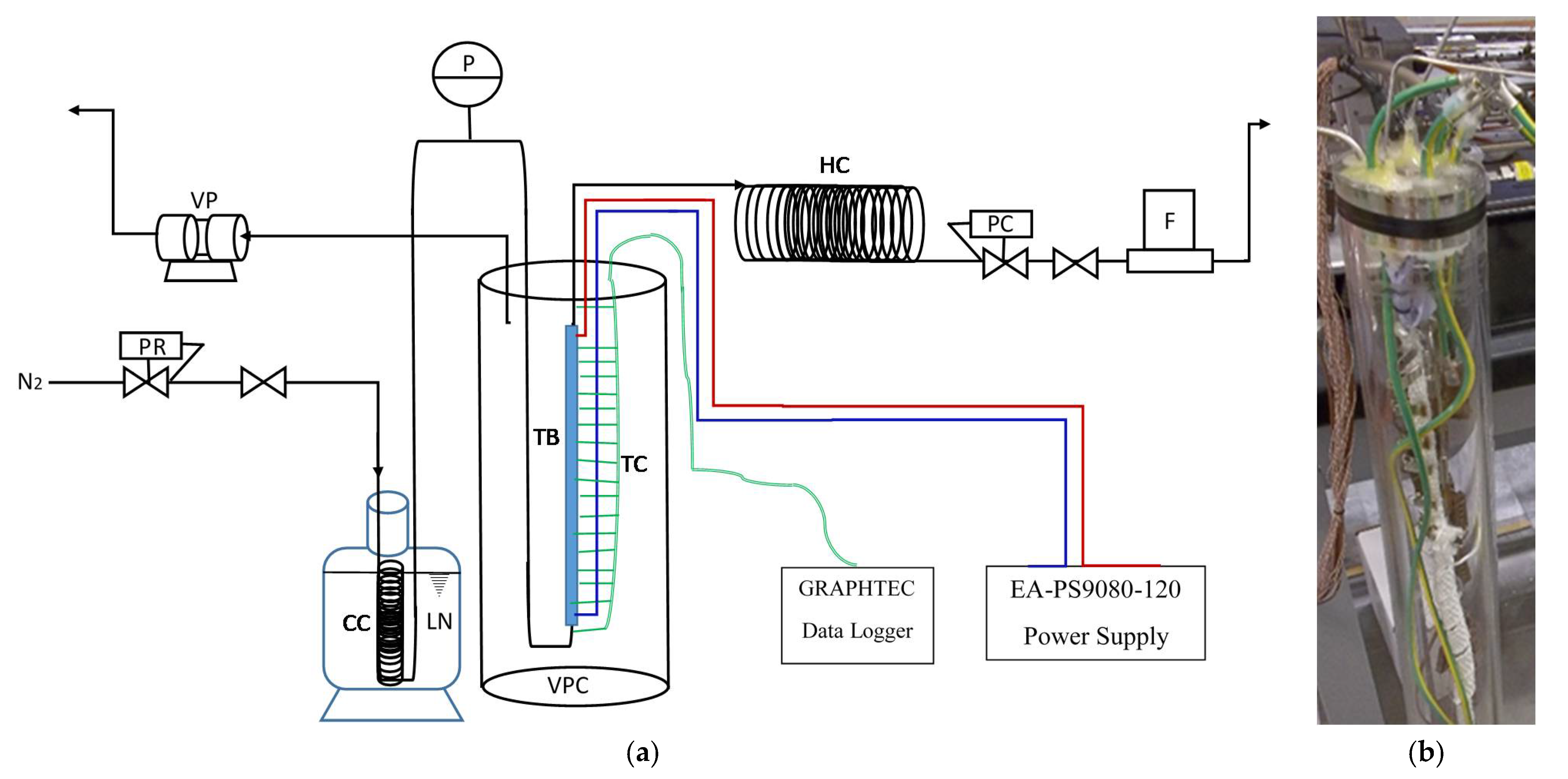
2. Experimental System and Procedures

The experimental system for characterizing the S-N2 heat transfer in a vertical tube is illustrated in Figure 2a. The main components of the system include a pressure regulator, cooling coil, liquid N2 tank, pressure gauge, circular straight tube test section, heating coil, gas flowmeter, data logger, power supply, etc. The pressure regulator (GAS ARC SPEC Master HPC6201, Speck and Burke, Alva, UK) was used to adjust the pressure of the N2 flow to the prescribed value while the cooling coil and the liquid N2 tank serve as a cryogenic source to cool the N2 flow to the prescribed temperature before entering the test section. As shown in Figure 2b, the test section includes an SS316 stainless steel test tube wrapped with fiberglass thermal insulation, which was vertically sitting inside a vacuum Perspex chamber. The vacuum was maintained by a vacuum pump (A134-51-912, Edward High Vacuum Speedivac 2, Edwards Limited, Burgess Hill, UK) which suppressed the heat losses for the test environment. The testing tube, with a length of 600 mm, an inner diameter of 2 mm, and a wall thickness of 0.5 mm, was heated by direct electric current provided via the Digital Bench Power Supply, creating a uniformly distributed heat flux on the tube surface. The N2 temperature and pressure were restored to room temperature and atmospheric pressure with the help of the heating coil and the pressure controller after exiting the test section, respectively.
A total of 28 Type-T thermocouples were welded onto the exterior surface of the testing tube at intervals of 20 mm while the distance between the first thermocouple and the tube inlet was 60 mm, for measuring the wall temperature of the heated tube under convective cooling [24]. At the tube inlet and outlet, another two Type-T thermocouples were installed to record the actual N2 fluid temperatures. The data from all thermocouples were gathered and stored by the data logger (Graphtec midi Logger GL840-M, Graphtec Corporation, Yokohama, Japan) for further analysis. The operating pressure of S-N2 was recorded via a pressure gauge mounted at the inlet of the test tube, while the flow rate was monitored through a gas flowmeter installed at a downstream position of the pressure controller. The physical variables used in the present study include pressure, mass flux and heat flux. The pressure was fixed by the pressure regulator. The mass flux was fixed by the pressure, inlet temperature, flowmeter and valve. The heat flux was fixed by the power supply. Table 1 lists the uncertainties and instruments of the experimental measurements.

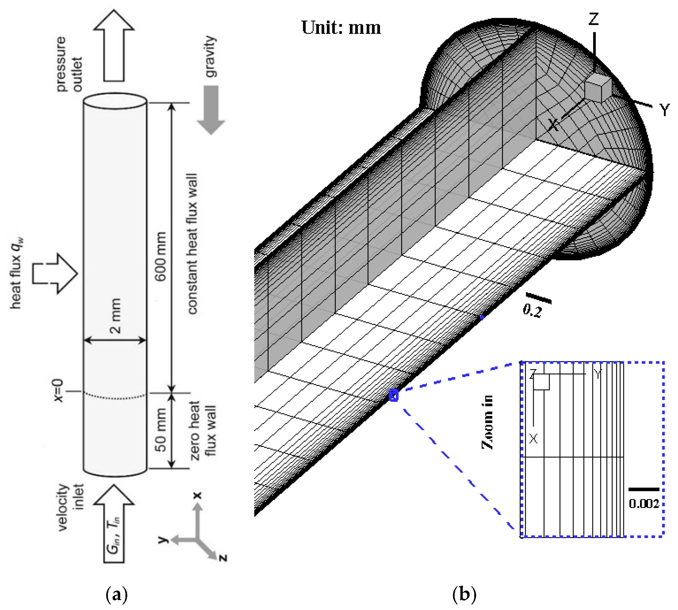
3. Numerical Model and Methodology

The computational domain and boundary conditions adopted in this study are as illustrated in Figure 3a. The total length of the tube as the computational domain was set to 650 mm. In the experiments, it was found that the N2 flow would be hydrodynamically fully developed before entering the test section. Accordingly, the first 50 mm of the computational domain (i.e., test tube) served as the developing length of the N2 flow, where the boundary condition was a zero heat flux wall, to create the same flow condition in the numerical simulations similar to that in the experiments. Same boundary conditions were applied to the rest segment of the computational tube as the test tube in the experiments, which was a constant and uniform wall heat flux condition. Uniform temperature and velocity profiles were employed as the condition at the tube inlet, while pressure condition was adopted at the tube outlet. In addition, the N2 flow in the tube was turbulent under the working conditions in this study. Two turbulence models, the standard k-ε model with enhanced wall treatment [20] and the SST k-ω model [21], were used and compared to seek the preferable model for predicting the turbulent convective heat transfer of S-N2 in the tube. The governing equations for this numerical simulation construct included the conservation equations of mass, momentum and energy and the transport equations of k and ε or ω, which are similar to those being used for general turbulent flow problems [25,26]. The equations governing continuity, momentum, and energy are as follows:
( ρ u i ) x i = 0  
( ρ u i u j ) x j = p x i + ρ g i + x j [ μ ( u i x j + u j x i ) u i u j ¯ ]  
( ρ u i c p T ) x i = x i [ λ T x i ρ c p u i T ¯ ]  
where u i u j ¯ and u i T ¯ are the turbulent stress tensor and turbulent heat flux vector, respectively [11].
The commercially available CFD software, ANSYS Fluent, was employed in this research to numerically study the turbulent convective heat transfer of S-N2 in the vertical tube. The governing equations were iteratively solved based on the steady pressure-based solver using the SIMPLE algorithm as the coupling scheme of pressure and velocity. The spatial discretization of gradient was implemented by the least-squares cell-based method for momentum, energy, and turbulent variables (k, ε, and ω) with the second-order upwind scheme. The convergence of the solving process was considered to be achieved when the normalized residuals of continuity, momentum, and energy equations decreased below 10−6. The thermophysical properties of N2 dependent on its temperature and pressure were considered and extracted from the NIST standard database [9] and fitted into the function expressions of temperature. The expressions were coded as user-defined functions (UDF), which were then compiled by Fluent and integrated into the solving process.
To obtain more reliable numerical results, a three-dimensional numerical model was established with the corresponding computational grids presented in Figure 3b. The whole computational region was discretized by the structured hexahedral mesh. Because of the abrupt changes of N2 thermophysical properties, it is of vital importance to delicately design the grids near the tube wall, i.e., to achieve a nondimensional wall distance y+ of lower than 1, so that the boundary layer can be precisely resolved, especially when a high Reynolds number flow relaminarized to a laminar flow due to the property variations. Consequently, the numerical grids close to the wall have been refined as Figure 3b shows. Furthermore, the independent study of grids was carried out to ensure adequate reliability of the simulation results. Comparison of average wall temperatures under four sets of grids is presented in Table 2. Considering the balance between accuracy and computational time, the finally determined number of grids was approximately 600,000 for all numerical simulations thereafter.

4. Results and Discussion

4.1. Data Processing and Uncertainty Analysis

The heat flux on the outer wall of the test tube q w o was given in the simulations. Therefore, the heat flux on the inner wall can be written as:
q = D d q w o
The system heat loss was considered in q w o for all the experiments, which was examined by comparing the enthalpy difference of N2 between the tube inlet and outlet with the total output power of the power supply. The enthalpy difference was calculated according to the measured N2 temperatures at the tube inlet and outlet. The resulting heat loss was lower than 10% of the total output power and such a small heat loss was attributed to the effective thermal insulation layer outside the tube wall. Based on the outer wall temperatures of the tube measured during the experiments, the inner wall temperatures can be obtained according to the heat conduction equation:
T w i ( x ) = T w o ( x ) q w o D ln ( D / d ) 2 λ t w
The local bulk fluid temperatures of N2 were looked up through the N2 thermophysical properties from the NIST database according to the local fluid enthalpies, which were determined based on the energy conservation law, in which the average enthalpy of the nitrogen at different axial locations within the test tube could be calculated as follows:
H ( x ) = H i n + 4 q G x d
The local heat transfer coefficient (LHTC) between the cold N2 and the inner wall of the heated tube along the flow direction was then obtained by:
h ( x ) = q T w i ( x ) T b ( x )
The uncertainty analysis of the experimental results was performed based on the multivariate propagation of error approach, which can be expressed as [24]:
σ h h = ( σ q q ) 2 + ( σ T w i T w i T b ) 2 + ( σ T b T w i T b ) 2
where σ h , σ q , σ T w i , and σ T b denote the uncertainties of h , q , T w i , and T b , respectively. The relative uncertainty of LHTC was calculated accordingly, which was around 12.5%.

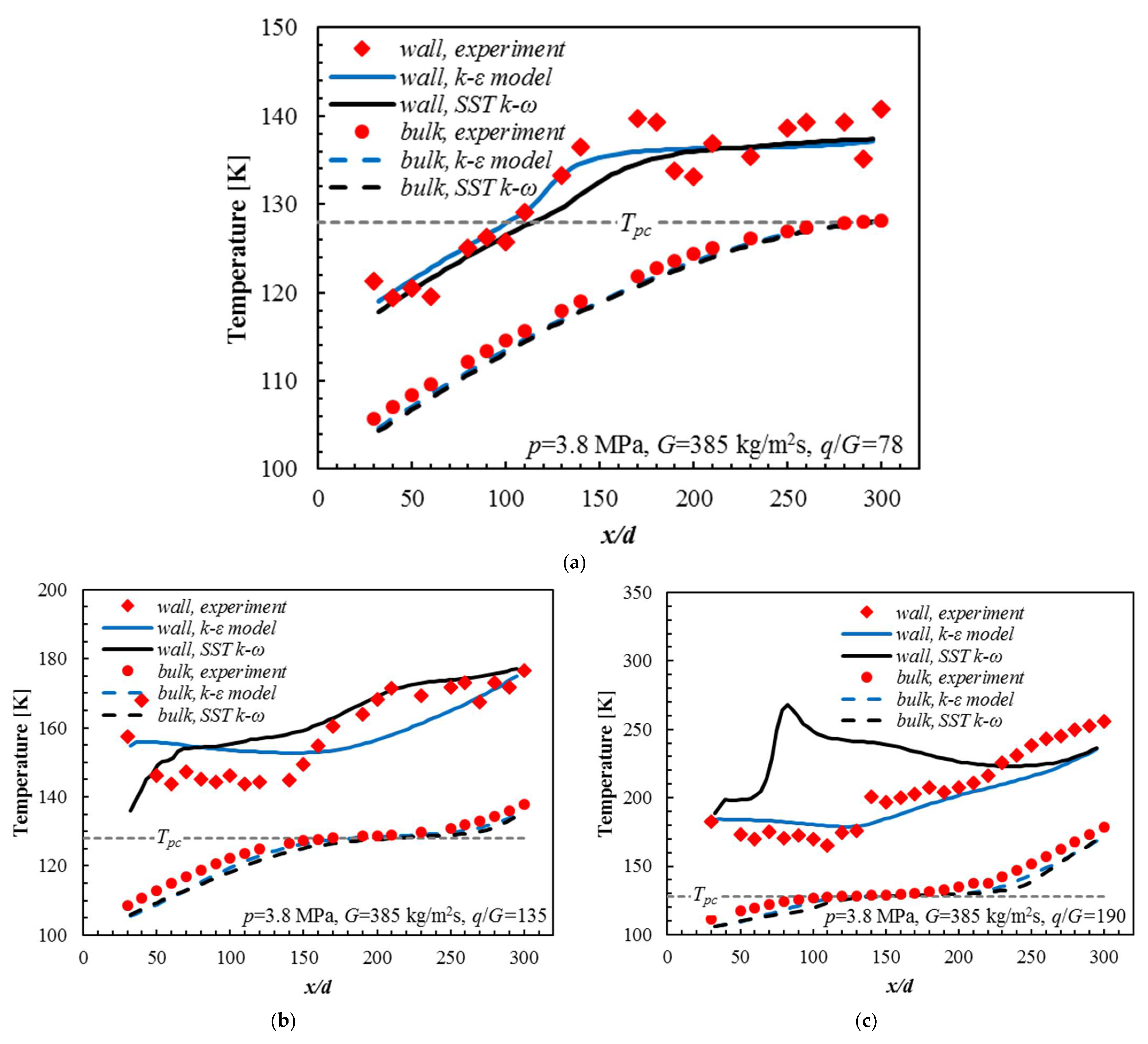
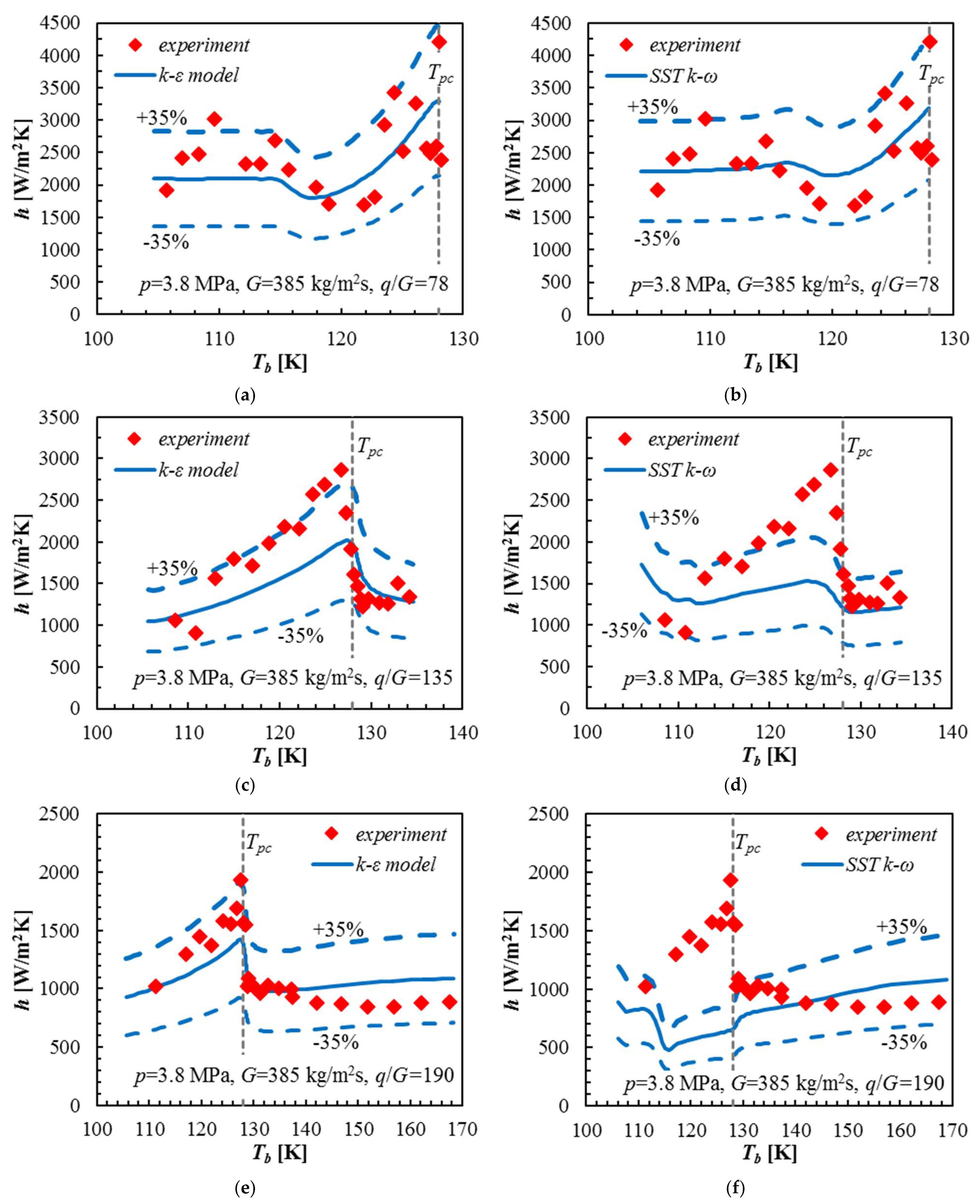
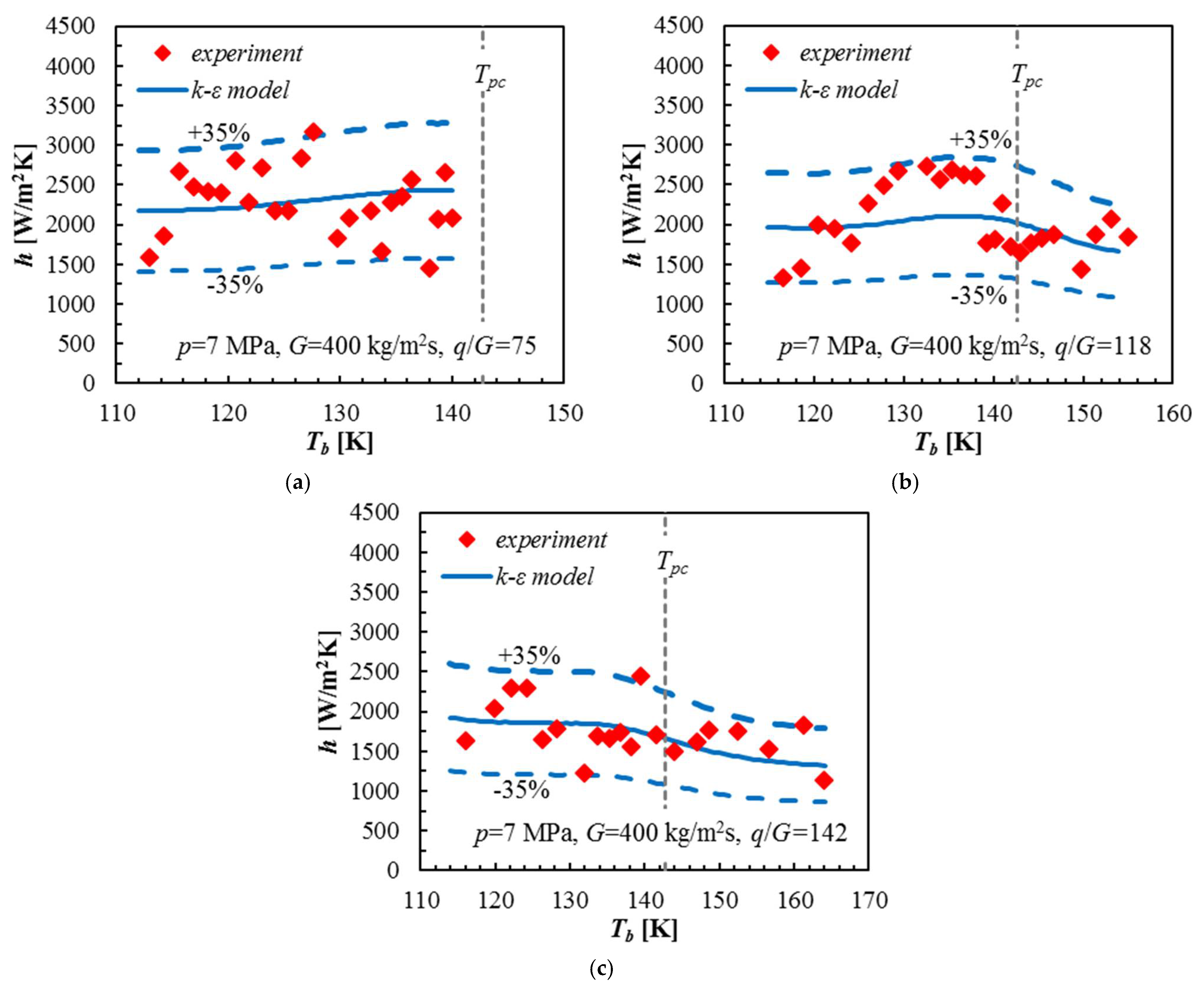
4.2. Comparison between Experimental and Numerical Results

Figure 4 compares the temperature profiles at the inner wall and of the bulk N2 fluid along the test tube between the experimental and simulation results with different turbulence models for various values of q / G at p = 3.8 MPa and G = 385 kg/m2 s. It can be observed that the bulk fluid temperatures of N2 obtained from simulations were consistent with the corresponding experimental values for all cases. While the bulk fluid temperature kept increasing along the flow direction, the increasing slope of the bulk fluid temperature was relatively small near T p c , and the position of the occurrence of these phenomena moves upstream with an increase in the heat flux. At a small heat flux ( q / G = 78 J/kg), the numerical wall temperature values computed from both turbulence models fairly coincided with the experimental values, although there was a small discrepancy between the numerical results themselves. In addition, when the heat flux increases, the wall temperature profile predicted by the k-ε model still agrees with the experimental results within an acceptable difference, whilst that predicted by the SST k-ω model considerably deviates from the experimental results, especially for the case of q / G = 190 J/kg. Furthermore, it can be noticed from the experiments that there was a unique slope change in the wall temperature profile (i.e., the temperature increase slows down) before the bulk temperature reached T p c , which is accurately predicted by the k-ε model for all cases. This could be mainly attributed to the sharp increase in the specific heat of N2 near T p c as illustrated in Figure 1a.
The comparisons of LHTC between experimental results and simulation results with different turbulence models for various values of q / G at p = 3.8 MPa and G = 385 kg/m2 s are shown in Figure 5. The LHTC was plotted as a function of the local bulk fluid temperature of the N2 flowing in the tube. As Figure 5 indicates, at a small heat flux ( q / G = 78 J/kg), the LHTCs originated from both the two turbulence models reasonably agree with the measured LHTCs within a relative deviation of ±35%. On the other hand, for higher heat fluxes ( q / G = 135 or 190 J/kg), this agreement was still found for the k-ε model, whereas the LHTC values predicted by the SST k-ω model was much less than the experimental values in a small region of T b < T p c where the relative deviation was considerably greater than 35%. It can be seen by further comparing the LHTC profiles that the k-ε model effectively reproduces the experimental characteristics for all the cases while the SST k-ω model fails to match with those for high heat fluxes ( q / G = 135 and 190 J/kg). Specifically, the experimental results show that the LHTC firstly increases to a maximum near T p c and then decreases significantly within a narrow range of T b at relatively high heat fluxes, which could be reproduced by the k-ε model with an acceptable deviation. Theoretically, it is not difficult to know that the maximum LHTC occurs at the minimum difference between T w i and T b , which happens near T p c as shown in Figure 4. Generally, LHTC is a positive correlation with c p , λ , and ρ . During T b increasing towards T p c , the c p dramatically increased, while the λ and ρ moderately decreased at p = 3.8 MPa as shown in Figure 1, and therefore the LHTC increased slowly. When T b more than T p c continued to increase, the c p dramatically decreased and the λ and ρ continued to decrease at p = 3.8 MPa, as shown in Figure 1, and therefore the LHTC decreased markedly, as Figure 5 shows. With the increase in q , the T b increased more in the same tube, which led to such significant differences between Figure 5a,c,e, although the maximum LHTC occurred near T p c in all the three cases. Overall, the results demonstrate that the standard k-ε model works well in predicting the convective heat transfer characteristics of S-N2 in a small vertical circular tube, outperforming the SST k-ω model.
To further validate the standard k-ε model, the comparison of LHTCs between experimental results and simulation results with the k - ε model for various values of q / G at p = 7 MPa and G = 400 kg/m2 s was conducted, as Figure 6 illustrates. The LHTCs predicted by the k-ε model again show an acceptable consistency with the experimental results for all the cases at p = 7 MPa, where all the relative deviations are within ±35%. Moreover, the basic trends of the measured LHTC changing along the tube length are also generally reproduced by the k-ε model for all the cases. Compared to the cases at p = 3.8 MPa, the LHTC at p = 7 MPa experiences a relatively smoother change with the increasing bulk fluid temperature, because of the less dramatic variations in N2 thermophysical properties.

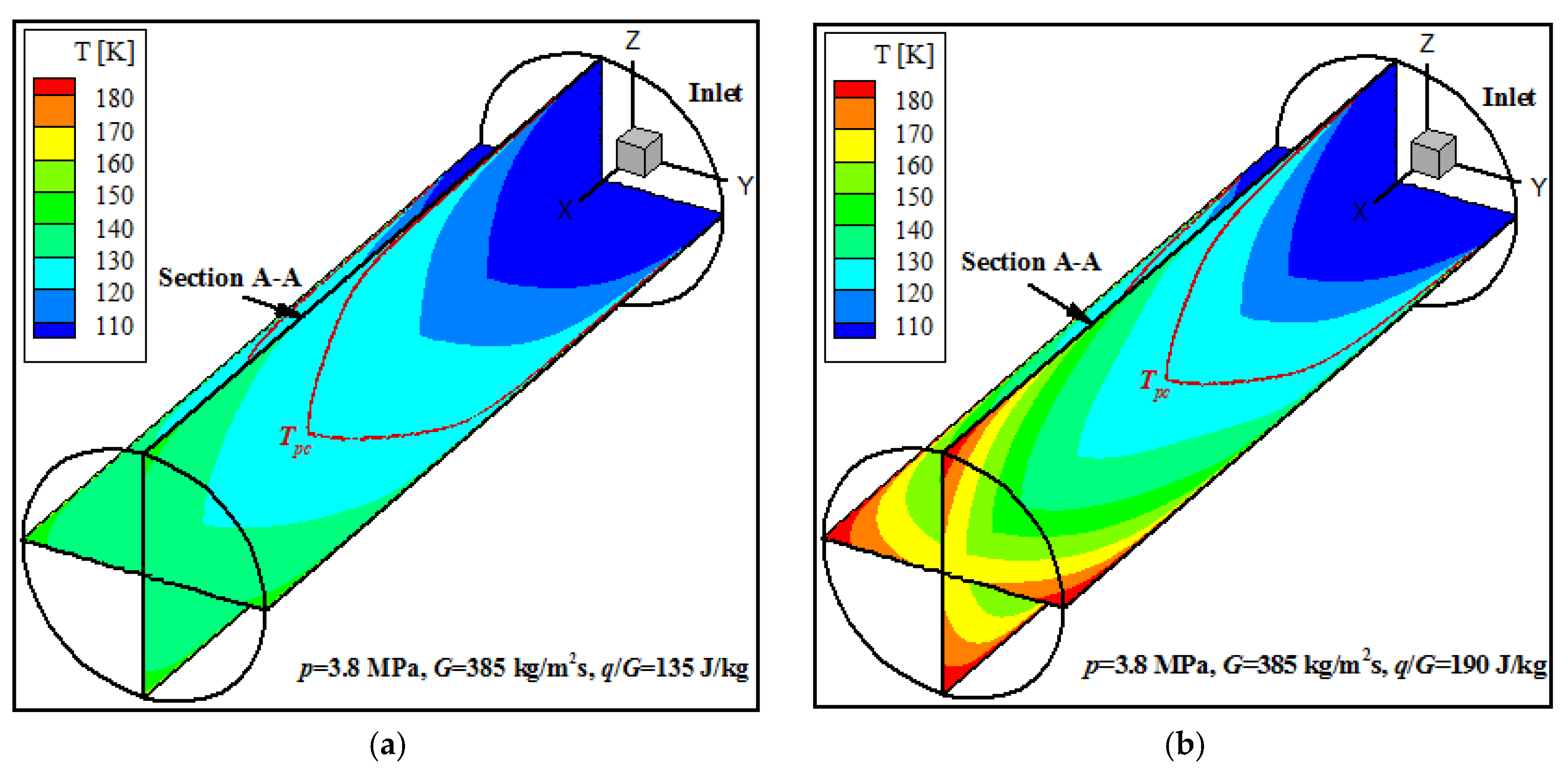
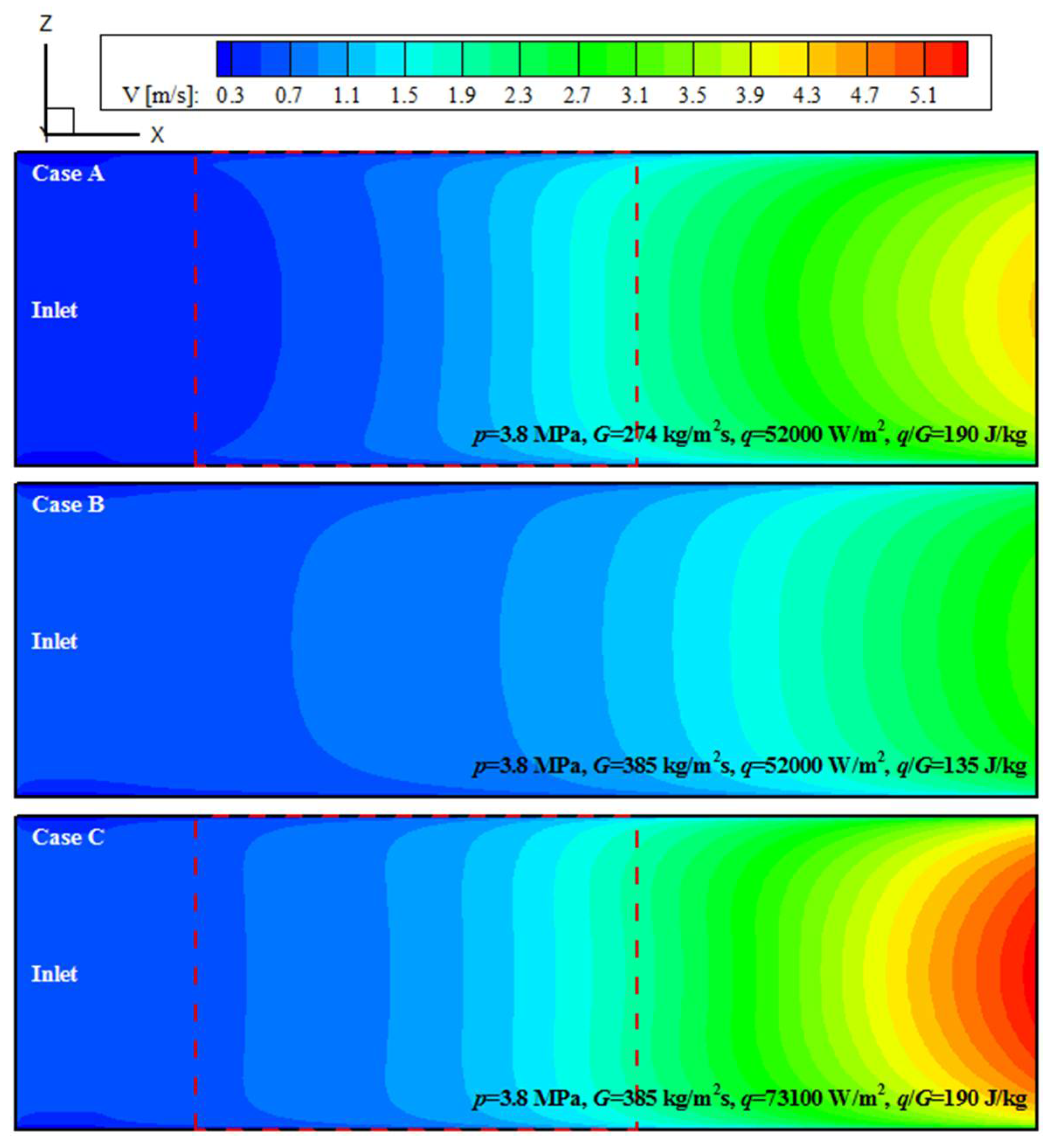
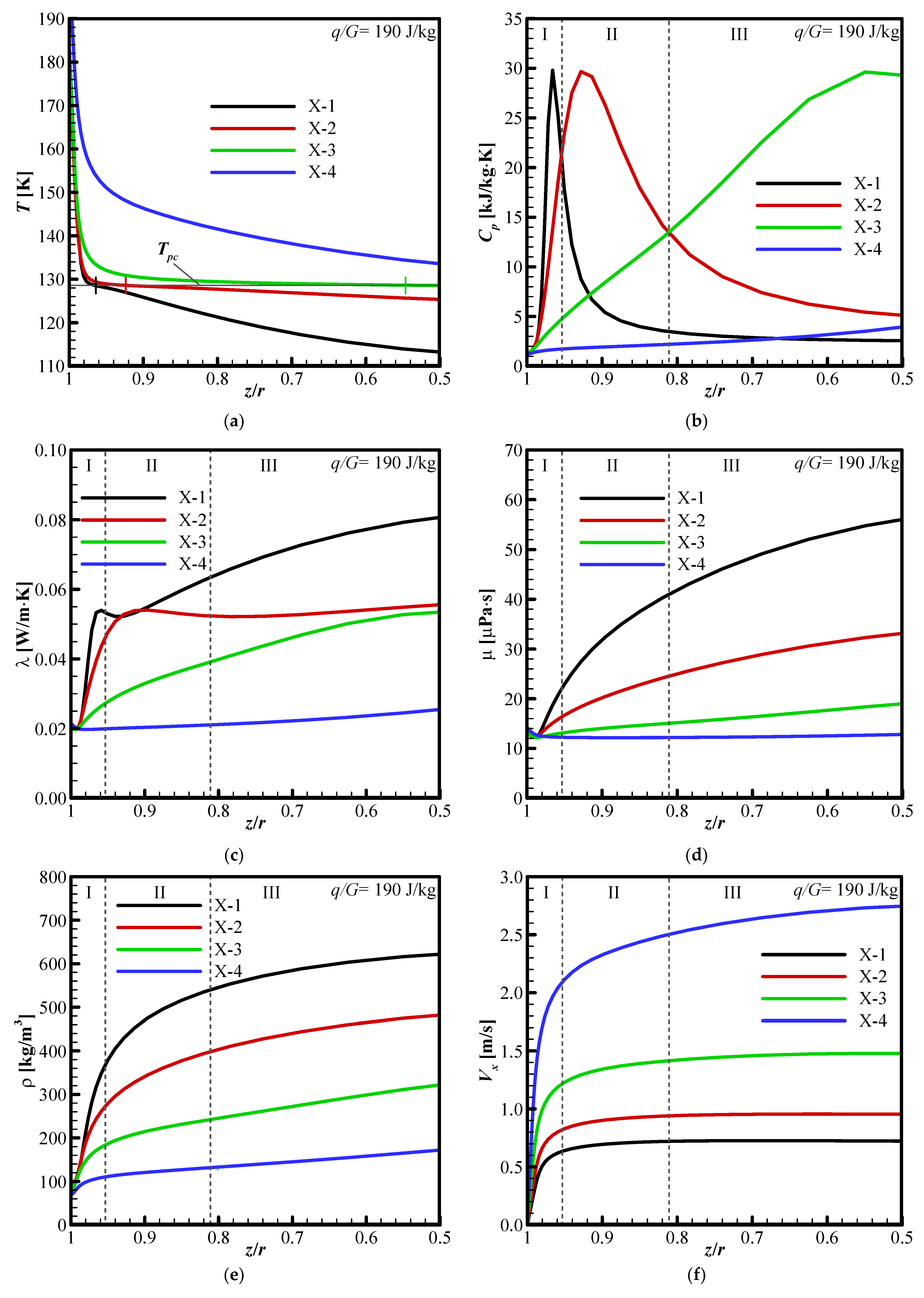
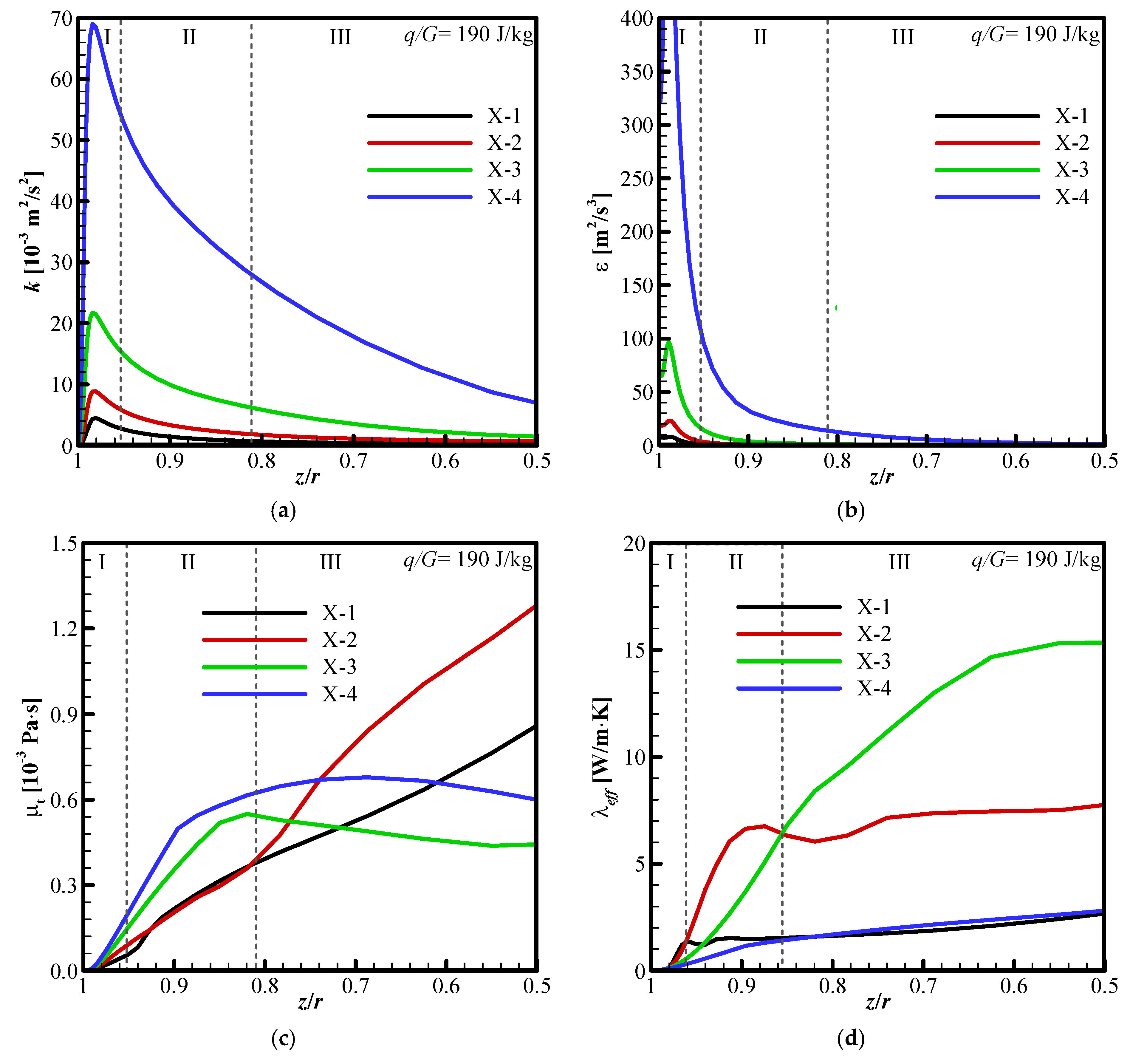
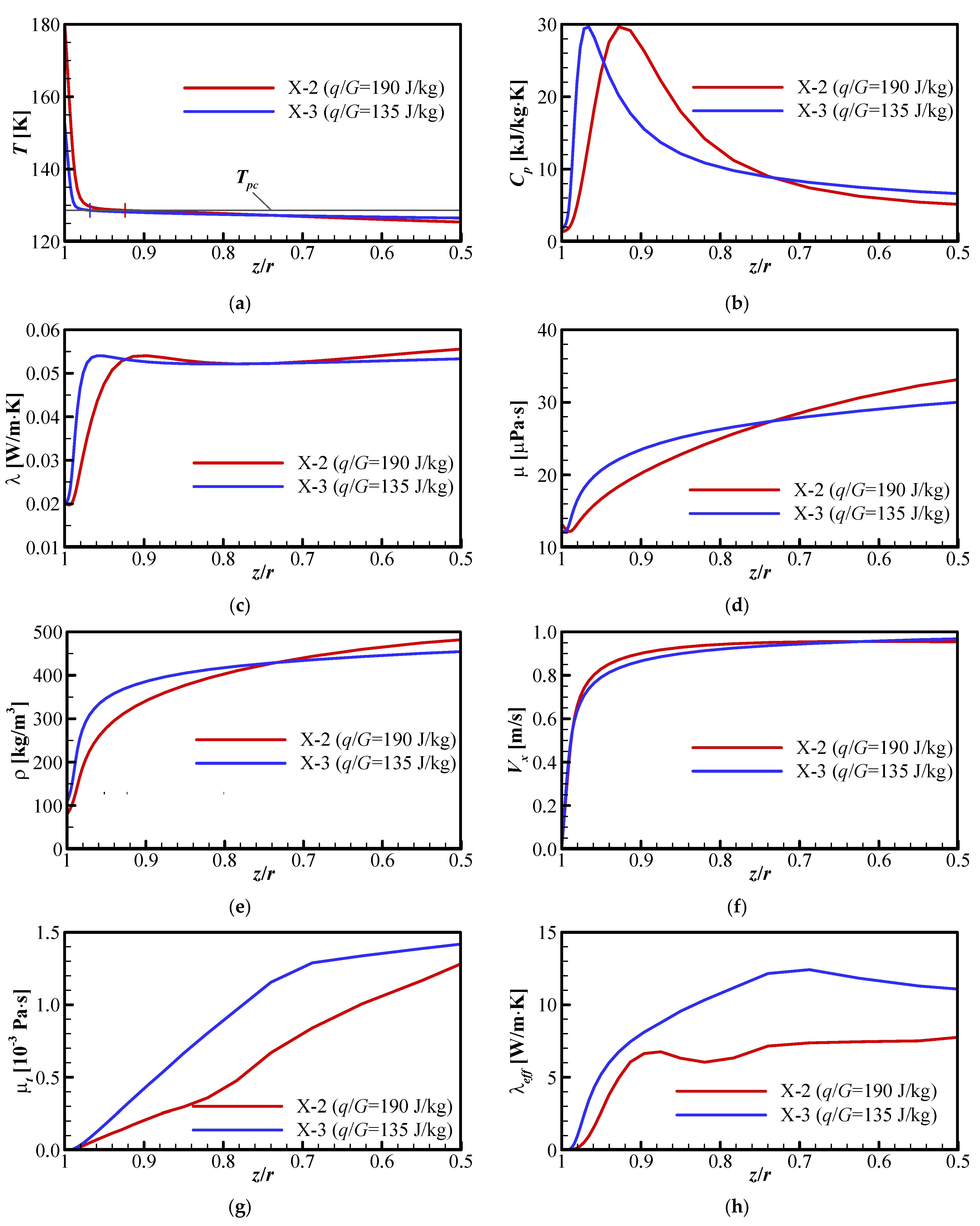
4.3. Analysis of Heat Transfer Characteristics

Since it is evident that the k-ε model is capable of effectively reproducing the heat transfer characteristics of N2 observed from the experiments, more simulations were carried out based on the k-ε model to further understand and explain the heat transfer characteristics of convective heat transfer of S-N2 in a small vertical tube under a series of varying conditions. The resulting profiles of LHTC along the flow direction for the cases with various values of q / G at p = 3.8 MPa and G = 385 kg/m2 s are shown in Figure 7a. As the figure shows, for a small heat flux ( q / G = 78 J/kg), the LHTC first decreased and then increased along the flow direction. At a moderate heat flux ( q / G = 119–146 J/kg), the LHTC first increased and then decreased. With the further increase of the heat flux ( q / G 168 J/kg), the HTC first increased and then decreased and slightly increased again before leaving the test tube. In addition, both the LHTC increasing slope and decreasing slope of all the LHTC profiles became flattened as the q / G value increased. The variations of the maximum LHTC and its corresponding location within the tube regarding different q / G values are further illustrated in Figure 7b. As shown in the figure, the maximum LHTC decreased with the increase in q / G while its corresponding location moved towards the tube inlet. Specifically, the maximum LHTC decreased from 3300 to 1400 W/m2·K as q / G increased from 78 to 190 J/kg.
The detailed temperature distributions inside the test tube were numerically visualized and are displayed in Figure 8, for two cases with different values of heat flux at p = 3.8 MPa and   G = 385 kg/m2·s. As indicated in the figure, in both cases, the N2 temperature increased from less than T p c to more than T p c , while the location of T p c moved from the tube wall and the tube centreline along a parabolic curve in the flow direction. The temperature gradient along the flow direction in the region near T p c was much less than those in other regions, which resulted from remarkably increased N2 specific heat in that region. Furthermore, by comparing the two cases, it can be found that the greater heat flux led to larger temperature gradients along both the axial and radial directions of the tube while the isothermal line of T p c moved towards the inlet and the centerline of the tube. Besides the change of q / G , the formation of new temperature distribution was attributed to its interaction with dramatically varying thermophysical properties of N2.
Figure 9 shows the velocity distributions (i.e., the isolines of the velocity magnitude) in Section A-A (see Figure 8) of the test tube for three cases with different mass fluxes or heat fluxes. In Case A, the velocity isolines within the region marked by the red dashed box are in saddle-like shape, which is attributed to the effect of buoyancy force. It means that the maximum velocity is located near the wall rather than in the centerline along the radial direction of the tube, which is quite different from a common case of flow in a circular tube. Moreover, compared to Case A, the effect of buoyancy force is effectively suppressed as presented in Case B due to the increased mass flux at the same heat flux. Furthermore, the comparison of the velocity isolines between Case B and Case C implies that a greater heat flux elevated the impact of buoyancy force. The velocity distributions in Figure 9 may be explained by considering the temperature distribution in Figure 8 and the temperature-dependent N2 density and viscosity in Figure 1 at the same time. It is suggested that the elevated buoyance force shrank the velocity difference between the fluid near the wall and near the centreline as shown in Case C, which thus inhibits the heat transfer along the radial direction [27]. Therefore, a higher heat flux may result in a stronger buoyancy effect, which could be one of the reasons for the weakened N2 heat transfer performance at higher heat fluxes as Figure 7a shows. By comparing Case A and Case C, it is clear that the effect of buoyancy force was also notably reduced by the increased mass flux even at the same q / G . Hence, the impact of buoyance force on heat transfer performance was weak or can even be ignored at high mass fluxes, which is consistent with the results of Zhu et al. [22]. The flow acceleration parameter, K v = 4 q D / ( R e b 2 μ b c p , b T b ) , was calculated for all cases and the calculated values were always lower than 3 × 10⁻⁶ in all cases. Therefore, the flow acceleration was not high enough to cause flow laminarization in the present study [20,21].
Four different cross-sections (i.e., axial locations X-1 to X-4 as shown in Figure 7a) were selected for comparative analysis to explain the variation of LHTC along the axial direction, taking the case with q / G = 190 J/kg as an example. The maximum LHTC occurred at X-2 while the minimum one occurred at X-4 in this case. Figure 10 and Figure 11 present radial variations of temperature, thermophysical properties and flow parameters of N2 within the region from z / r = 1 to 0.5 on the four selected cross-sections in this case. z / r = 1 and 0 denote the wall and the centerline of the tube, respectively. As marked in Figure 10a, the N2 temperature gradually decreased to less than T p c along the radial direction away from the wall on X-1, X-2 and X-3, while it is above T p c within the whole region on X-4. The position of reaching T p c moved towards the centerline as the axial location moves from X-1 towards X-3. Combined with Figure 7a, it can be found that when T p c appears in the boundary layer adjacent to the wall, the LHTC began to increase and heat transfer enhancement was initiated. When T p c moved along the radial direction to a certain position within the boundary layer, LHTC reached its maximum. When T p c moved outside the boundary layer, significant heat transfer deterioration occurred. The specific heat ( c p ) varied sharply between 1 and 30 kJ/kg·K and reached the maximum at the position of reaching T p c on the three cross-sections, while it varied slightly between 1 and 4 kJ/kg·K on X-4, much smaller than that on other cross-sections as shown in Figure 10b. For convenience, the whole region was artificially divided into three subregions. Compared to other cross-sections, c p was larger on X-1 in Subregion I, on X-2 in Subregion II, but on X-3 in Subregion III. The thermal conductivity ( λ ), viscosity ( μ ) and density ( ρ ) all decreased nearly in the whole region except for some very small local zones when the cross-section moves from X-1 towards X-4 (see Figure 10c–e). The reduction of ρ and μ increases axial flow velocity ( V x ) and near-wall velocity gradients ( V x / r ) as Figure 10f shows. Although different buoyancy forces caused by different radial density gradients change the velocity distributions near the wall for different cross-sections, the changes are not significant in this case.
Since its generation was directly related to the velocity gradient, the turbulent kinetic energy ( k ) increased from X-1 towards X-4 (see Figure 11a). However, the turbulent dissipation rate ( ε ) also rises as Figure 11b shows. Since the turbulent viscosity ( μ t ) can be expressed as μ t = c μ ρ k 2 / ε where c μ is a constant [28,29], the combined effect of ρ , k and ε results in notably different profiles of μ t among the four cross-sections as Figure 11c presents. Further, the effective thermal conductivity can be written as λ e f f = λ + μ t P r t c p , where the turbulent Prandtl number ( P r t ) is nearly constant [28,30]. The resulting profiles of λ e f f are illustrated in Figure 11d where the whole region is re-divided into three subregions slightly different from Figure 10b. It is well known that the thermal resistance in the near-wall region is of vital importance to the LHTC for the tube flow with a heated wall. Since the fluid in the region away from the wall also transfers and carries heat, the thermal resistance there should also be considered in understanding the LHTC. In comparison with X-2, although λ e f f on X-1 is slightly larger in Subregion I near the wall and λ e f f on X-3 is higher in Subregion III away from the wall, λ e f f on X-1 is much smaller in Subregions II and III and λ e f f on X-3 is lower in Subregions I and II. λ e f f on X-4 is much lower in Subregions I and II than those on other cross-sections while it still maintains a very lower level in Subregion III. Considering the combined effects of the dominated λ e f f in the region near the wall and the secondary λ e f f in the region away from the wall, the LHTC was therefore the largest at X-2 and the lowest at X-4 for the case with q / G = 190 J/kg. By comparing Figure 10b and Figure 11d, it can be found that which cross-section has a larger λ e f f at the same radial position is mainly determined by the corresponding c p . Moreover, it can be found that the turbulent kinetic energy decreases with the increase of density from Figure 10e and Figure 11a.
To further understand the variation of maximum LHTC with q / G at a constant G , radial variations of various thermophysical properties and flow parameters of N2 at axial locations corresponding to maximum LHTCs for the cases with q / G = 190 J/kg and q / G = 135 J/kg were comparatively analyzed as examples, as shown in Figure 12. The maximum LHTC occurred at the axial location X-2 for the case with q / G = 190 J/kg while it occurs at the axial location X-3 for the case with q / G = 135 J/kg (see Figure 7a). As Figure 12a shows, the N2 temperature on X-2 of the case with   q / G = 190 J/kg rises more sharply from the tube centreline to the wall and reaches T p c farther from the wall than that on X-3 of the case with   q / G = 135 J/kg. Hence, both c p and λ near the wall on X-3 varied more drastically and were higher than those on X-2, although they had similar radial changing tendencies and the same maximums at the two axial locations (see Figure 12b,c). Since μ was slightly smaller near the wall and the variation of ρ was slightly larger near the wall resulting in higher buoyance forces, the near-wall velocity gradients ( V x / r ) were slightly higher on X-2 of the case with   q / G = 190 J/kg as shown in Figure 10d–f. Since its generation was directly related to velocity gradients, k near the wall on X-2 was larger compared to X-3, but the situation was reversed near the centerline, while ε near the wall on X-2 was also larger but its difference near the centreline between the two locations almost vanishes (not shown). Likewise, the combined effect of ρ , k , and ε results in a larger value of μ t on X-3 compared to X-2 within the whole region (see Figure 12g), since λ e f f = λ + μ t P r t c p , λ e f f on X-3 of the case with   q / G = 135 J/kg was always larger than that X-2 of the case with   q / G = 190 J/kg as presented in Figure 12h. As a result, the maximum LHTC for the case with   q / G = 135 J/kg was larger than that for the case with   q / G = 190 J/kg. By comparing Figure 12g,h, it can be found that which q / G case has a larger λ e f f corresponding to the maximum LHTC is mainly determined by the corresponding μ t .

5. Conclusions

This paper studied the convective heat transfer behaviors of S-N2 flowing upward in a small vertical tube by experimental measurements and numerical simulations based on different turbulence models with emphatically analyzing the formation mechanism of complicated heat transfer characteristics in detail. By comparing the results, it was demonstrated that the standard k-ε model with enhanced wall treatment was superior to the SST k-ω model. The former could effectively predict the key heat transfer characteristics of S-N2 under wide working conditions, while the latter failed to follow up especially for the high q / G cases.
The local heat transfer performance of S-N2 underwent considerable and nonmonotonic variation along the flow direction, which was undoubtedly attributed to drastically varying thermophysical properties of N2 with temperature. The variation mechanism of LHTC along the flow direction can be explained by effective thermal conductivity, which is related to thermal conductivity, specific heat, and turbulent viscosity. The maximum (minimum) LHTC occurred at the axial location of the tube where the effective thermal conductivity in a wide enough radial region near the tube wall was the largest (lowest) among all axial locations. The radial profile differences of effective thermal conductivity between different axial locations of the tube were mainly determined by the radial profile of specific heat. The maximum LHTC decreases with the increase in q / G at a constant G , which owes to the decreased effective thermal conductivity in a wide enough radial region near the tube wall. The decrease of effective thermal conductivity corresponding to the maximum LHTC was mainly caused by the decrease of turbulent viscosity as q / G increased.
It is necessary to further investigate S-N2 convective heat transfer in a heated tube under a wider range of conditions, different tube geometries, inner fin, and inserts by both experimental and numerical methods, in order to obtain more information about the characteristics and enhancement methods of S-N2 heat transfer. The research will provide a guidance for the design of S-N2 heat exchanger in LAES systems.

Author Contributions

Conceptualization, Y.L.; methodology, Q.Y.; software, C.C.N.; validation, Y.P. and C.C.N.; formal analysis, Q.Y.; investigation, Q.Y. and C.C.N.; resources, Q.Y. and Y.L.; data curation, Y.P.; writing—original draft preparation, Q.Y. and Y.P.; writing—review and editing, Q.Y. and Y.W.; visualization, Y.W.; supervision, Y.L.; project administration, Y.L.; funding acquisition, Y.L. All authors have read and agreed to the published version of the manuscript.

Funding

This research was funded by the Engineering and Physical Sciences Research Council (EPSRC) of the United Kingdom, grant number EP/N021142/1.

Conflicts of Interest

The authors declare no conflict of interest.

Nomenclature

Roman letters
c p specific heat (kJ·kg−1·K−1)
d inner diameter (mm)
D outer diameter (mm)
G mass flux (kg·m−2·s−1)
h heat transfer coefficient (W·m−2·K−1)
H enthalpy (kJ·kg−1)
N u Nusselt number
p pressure (MPa)
P r Prandtl number
q heat flux (W·m−2)
r inner radius (mm)
R e Reynolds number
T temperature (K)
u velocity (m·s−1)
V x axial flow velocity (m·s−1)
x axial distance from the inlet (mm)
y + non-dimensional wall distance
Greek letters
ε turbulent dissipation rate (m−2·s−3)
k turbulent kinetic energy (m−2·s−2)
λ thermal conductivity (W·m−1·K−1)
μ dynamic viscosity (Pa·s)
ρ density (kg·m−3)
Subscripts
b bulk
c critical
e f f effective
i n inlet
p c pseudo-critical
w i inner wall
w o outer wall
t turbulent
t w tube wall
Abbreviations
LAESliquid air energy storage
LHTClocal heat transfer coefficient
LNGliquefied natural gas
S-CO2supercritical carbon dioxide
S-N2supercritical nitrogen

References

  1. Legrand, M.; Rodríguez-Antón, L.M.; Martinez-Arevalo, C.; Gutiérrez-Martín, F. Integration of liquid air energy storage into the spanish power grid. Energy 2019, 187, 115965. [Google Scholar] [CrossRef]
  2. She, X.; Zhang, T.; Cong, L.; Peng, X.; Li, C.; Luo, Y.; Ding, Y. Flexible integration of liquid air energy storage with liquefied natural gas regasification for power generation enhancement. Appl. Energy 2019, 251, 113355. [Google Scholar] [CrossRef]
  3. Peng, H.; Shan, X.; Yang, Y.; Ling, X. A study on performance of a liquid air energy storage system with packed bed units. Appl. Energy 2018, 211, 126–135. [Google Scholar] [CrossRef]
  4. Nakhchi, M.E.; Esfahani, J.A. Improving the melting performance of PCM thermal energy storage with novel stepped fins. J. Energy Storage 2020, 30, 101424. [Google Scholar] [CrossRef]
  5. Lee, I.; Park, J.; Moon, I. Conceptual design and exergy analysis of combined cryogenic energy storage and LNG regasification processes: Cold and power integration. Energy 2017, 140, 106–115. [Google Scholar] [CrossRef]
  6. Zhang, T.; Chen, L.; Zhang, X.; Mei, S.; Xue, X.; Zhou, Y. Thermodynamic analysis of a novel hybrid liquid air energy storage system based on the utilization of LNG cold energy. Energy 2018, 155, 641–650. [Google Scholar] [CrossRef]
  7. Dondapati, R.S.; Ravula, J.; Thadela, S.; Usurumarti, P.R. Analytical approximations for thermophysical properties of supercritical nitrogen (SCN) to be used in futuristic high temperature superconducting (HTS) cables. Phys. C Supercond. Its Appl. 2015, 519, 53–59. [Google Scholar] [CrossRef]
  8. Mahdavi, M.; Yousefzade, O.; Garmabi, H. A simple method for preparation of microcellular PLA/calcium carbonate nanocomposite using super critical nitrogen as a blowing agent: Control of microstructure. Adv. Polym. Technol. 2018, 37, 3017–3026. [Google Scholar] [CrossRef]
  9. NIST Chemistry WebBook. Available online: http://webbook.nist.gov/chemistry/fluid/ (accessed on 15 June 2021).
  10. Pioro, I.L. Current status of research on heat transfer in forced convection of fluids at supercritical pressures. Nucl. Eng. Des. 2019, 354, 110207. [Google Scholar] [CrossRef]
  11. Wang, Z.; Qi, G.; Li, M. Numerical Investigation of Heat Transfer to Supercritical Water in Vertical Tube under Semicircular Heating Condition. Energies 2019, 12, 3958. [Google Scholar] [CrossRef] [Green Version]
  12. Chen, S.; Gu, H.; Liu, M.; Xiao, Y.; Cui, D. Experimental investigation on heat transfer to supercritical water in a three-rod bundle with spacer grids. Appl. Therm. Eng. 2020, 164, 114466. [Google Scholar] [CrossRef]
  13. Zhang, S.; Xu, X.; Liu, C.; Liu, X.; Dang, C. Experimental investigation on the heat transfer characteristics of supercritical CO2 at various mass flow rates in heated vertical-flow tube. Appl. Therm. Eng. 2019, 157, 113687. [Google Scholar] [CrossRef]
  14. Ren, Z.; Zhao, C.-R.; Jiang, P.-X.; Bo, H.-L. Investigation on local convection heat transfer of supercritical CO2 during cooling in horizontal semicircular channels of printed circuit heat exchanger. Appl. Therm. Eng. 2019, 157, 113697. [Google Scholar] [CrossRef]
  15. Lei, X.; Zhang, J.; Gou, L.; Zhang, Q.; Li, H. Experimental study on convection heat transfer of supercritical CO2 in small upward channels. Energy 2019, 176, 119–130. [Google Scholar] [CrossRef]
  16. Wang, J.; Li, J.; Gurgenci, H.; Veeraragavan, A.; Kang, X.; Hooman, K. Computational investigations on convective flow and heat transfer of turbulent supercritical CO2 cooled in large inclined tubes. Appl. Therm. Eng. 2019, 159, 113922. [Google Scholar] [CrossRef]
  17. Tian, R.; Wei, M.; Dai, X.; Song, P.; Shi, L. Buoyancy effect on the mixed convection flow and heat transfer of supercritical R134a in heated horizontal tubes. Int. J. Heat Mass Transf. 2019, 144, 118607. [Google Scholar] [CrossRef]
  18. Yu, Q.; Song, W.; Al-Duri, B.; Zhang, Y.; Xie, D.; Ding, Y.; Li, Y. Theoretical analysis for heat exchange performance of transcritical nitrogen evaporator used for liquid air energy storage. Appl. Therm. Eng. 2018, 141, 844–857. [Google Scholar] [CrossRef]
  19. Dimitrov, D.; Zahariev, A.; Kovachev, V.; Wawryk, R. Forced convective heat transfer to supercritical nitrogen in a vertical tube. Int. J. Heat Fluid Flow 1989, 10, 278–280. [Google Scholar] [CrossRef]
  20. Negoescu, C.C.; Li, Y.L.; Al-Duri, B.; Ding, Y.L. Heat transfer behaviour of supercritical nitrogen in the large specific heat region flowing in a vertical tube. Energy 2017, 134, 1096–1106. [Google Scholar] [CrossRef] [Green Version]
  21. Zhang, P.; Huang, Y.; Shen, B.; Wang, R.Z. Flow and heat transfer characteristics of supercritical nitrogen in a vertical mini-tube. Int. J. Therm. Sci. 2011, 50, 287–295. [Google Scholar] [CrossRef]
  22. Zhu, X.; Lyu, Z.; Yu, X.; Li, Q.; Cao, M.; Ren, Y. Heat Transfer Enhancement of Supercritical Nitrogen Flowing Downward in a Small Vertical Tube: Evaluation of System Parameter Effects. J. Therm. Sci. 2020, 29, 1487–1503. [Google Scholar] [CrossRef]
  23. Wang, Y.; Lu, T.; Drögemüller, P.; Yu, Q.; Ding, Y.; Li, Y. Enhancing deteriorated heat transfer of supercritical nitrogen in a vertical tube with wire matrix insert. Int. J. Heat Mass Transf. 2020, 162, 120358. [Google Scholar] [CrossRef]
  24. Nouri-Borujerdi, A.; Nakhchi, M.E. Experimental study of convective heat transfer in the entrance region of an annulus with an external grooved surface. Exp. Therm. Fluid Sci. 2018, 98, 557–562. [Google Scholar] [CrossRef]
  25. He, S.; Jiang, P.-X.; Xu, Y.-J.; Shi, R.-F.; Kim, W.S.; Jackson, J.D. A computational study of convection heat transfer to CO2 at supercritical pressures in a vertical mini tube. Int. J. Therm. Sci. 2005, 44, 521–530. [Google Scholar] [CrossRef]
  26. ANSYS. ANSYS Fluent Theory Guide; ANSYS, Inc.: Canonsburg, PA, USA, 2013. [Google Scholar]
  27. Huang, D.; Li, W. A brief review on the buoyancy criteria for supercritical fluids. Appl. Therm. Eng. 2018, 131, 977–987. [Google Scholar] [CrossRef]
  28. Sahu, S.; Vaidya, A.M. Numerical study of enhanced and deteriorated heat transfer phenomenon in supercritical pipe flow. Ann. Nucl. Eng. 2020, 135, 106966. [Google Scholar] [CrossRef]
  29. Launder, B.E.; Spalding, D.B. The numerical computation of turbulent flows. Comput. Methods Appl. Mech. Eng. 1974, 3, 269–289. [Google Scholar] [CrossRef]
  30. Tang, G.; Shi, H.; Wu, Y.; Lu, J.; Li, Z.; Liu, Q.; Zhang, H. A variable turbulent Prandtl number model for simulating supercritical pressure CO2 heat transfer. Int. J. Heat Mass Transf. 2016, 102, 1082–1092. [Google Scholar] [CrossRef]
Figure 1. Variations of thermophysical properties of N2 with temperature: (a) density and specific heat capacity; (b) viscosity and thermal conductivity [9].
Energies 14 07773 g001
Figure 2. Schematics of the experimental system (a) and real picture of the test section (b). VP—vacuum pump; PR—pressure regulator; CC—cooling coil; LN—liquid N2; P—pressure gauge; TB—test tube; VPC—vacuum Perspex chamber; TC—thermocouples; HC—heating coil; PC—pressure controller; F—gas flowmeter.
Energies 14 07773 g002
Figure 3. Physical model (a) and computational grids with local enlarged boundary layer (b).
Energies 14 07773 g003
Figure 4. Comparison of the inner wall and bulk fluid temperature profiles along the tube between experimental and simulation results with different turbulence models for various values of q / G (Unit: J/kg) at p = 3.8 MPa and T i n = 101 K: (a) q / G = 78; (b) q / G = 135; and (c) q / G = 190.
Energies 14 07773 g004
Figure 5. Comparisons of LHTCs between experimental results and simulation results with different turbulence models for various values of q / G (Unit: J/kg) at p = 3.8 MPa and T i n = 101 K: (a) q / G = 78 with k-ε model; (b) q / G = 78 with SST k-ω model; (c) q / G = 135 with k-ε model; (d) q / G = 135 with SST k-ω model; (e) q / G = 190 with k-ε model; and (f) q / G = 190 with SST k-ω model. The blue dash lines represent ±35% deviations with respect to the blue solid line (i.e., simulation results).
Energies 14 07773 g005
Figure 6. Comparisons of LHTCs between experimental results and simulation results with k - ε model for various values of q / G (Unit: J/kg) at p = 7 MPa and T i n = 110 K: (a) q / G = 75; (b) q / G = 118; and (c) q / G = 142. The blue dash lines represent ±35% deviations with respect to the blue solid line (i.e., simulation results).
Energies 14 07773 g006
Figure 7. LHTCs of N2 at p = 3.8 MPa and T i n = 101 K for various values of q / G : (a) their variations along the test tube axis; (b) maximum LHTCs and the corresponding locations in the tube.
Energies 14 07773 g001
Figure 8. Temperature distributions within the test on the XZ and XY planes (X:Y:Z = 1:100:100) for the numerical cases at p = 3.8 MPa, G = 385 kg/m2·s, and T i n = 101 K with different values of q / G : (a) q / G = 135; and (b) q / G = 190. The red line indicates the isothermal line of T p c .
Energies 14 07773 g008
Figure 9. Comparison of velocity distributions in Section A-A (X:Z = 1:100) of the test tube at p = 3.8 MPa and T i n = 101 K among the cases with different values of   G or q .
Energies 14 07773 g009
Figure 10. Radial variations at four different axial locations for the case with q / G = 190 J/kg at p = 3.8 MPa and G = 385 kg/m2·s: (a) temperature; (b) specific heat; (c) thermal conductivity; (d) viscosity; (e) density; and (f) axial velocity. z / r = 1 and 0 denote the wall and centerline of the tube, respectively.
Energies 14 07773 g010
Figure 11. Radial variations at four different axial locations for the case with q / G = 190 J/kg at p = 3.8 MPa and G = 385 kg/m2·s: (a) turbulent kinetic energy; (b) turbulent dissipation rate; (c) turbulent viscosity; (d) effective thermal conductivity. z / r = 1 and 0 denote the wall and centreline of the tube, respectively.
Energies 14 07773 g011
Figure 12. Radial variations at four different axial locations for the case with q / G   = 190 J/kg at p   = 3.8 MPa and G = 385 kg/m2·s: (a) temperature; (b) specific heat; (c) thermal conductivity; (d) viscosity; (e) density; (f) axial velocity; (g) turbulent viscosity; and (h) effective thermal conductivity. z / r = 1 and 0 denote the wall and centreline of the tube, respectively.
Energies 14 07773 g012
Table 1. The uncertainties and instruments of measured parameters.
Measured ParameterUncertaintyInstrumentsSpecifications
Power±1 WDigital Bench Power Supply, EA-PS 9080-120 2U, Elektro-Automatik Analogue, Viersen, Germany<0.1% of read value
<0.002 Volt
<0.08 Ampere
Flow rate±0.3 L/minOmega FMA-A2323 digital flowmeter, OMEGA Engineering Inc., Norwalk, CT, USA±1% of full scale
±0.3 SLM
Temperature±0.5 °CType-T thermocouple, Thermon Ltd., London, UK±0.5 °C
Pressure±0.05 barAlicat Scientific pressure measuring and controller, PCH-1000PSIA-D-PCA14, Alicat Scientific, Tucson, AZ, USA±0.125% of read value
Length±1 mm ±1 mm of length
Diameter±0.1 mm ±0.1 mm of diameter
Table 2. Average wall temperature under four sets of grids.
Number of grids150,000300,000600,0001200,000
Average wall temperatures160.25 K161.12 K161.61 K161.93 K
Publisher’s Note: MDPI stays neutral with regard to jurisdictional claims in published maps and institutional affiliations.

