Hybrid Machine Learning Approaches and a Systematic Model Selection Process for Predicting Soot Emissions in Compression Ignition Engines

Abstract

The standards for emissions from diesel engines are becoming more stringent and accurate emission modeling is crucial in order to control the engine to meet these standards. Soot emissions are formed through a complex process and are challenging to model. A comprehensive analysis of diesel engine soot emissions modeling for control applications is presented in this paper. Physical, black-box, and gray-box models are developed for soot emissions prediction. Additionally, different feature sets based on the least absolute shrinkage and selection operator (LASSO) feature selection method and physical knowledge are examined to develop computationally efficient soot models with good precision. The physical model is a virtual engine modeled in GT-Power software that is parameterized using a portion of experimental data. Different machine learning methods, including Regression Tree (RT), Ensemble of Regression Trees (ERT), Support Vector Machines (SVM), Gaussian Process Regression (GPR), Artificial Neural Network (ANN), and Bayesian Neural Network (BNN) are used to develop the black-box models. The gray-box models include a combination of the physical and black-box models. A total of five feature sets and eight different machine learning methods are tested. An analysis of the accuracy, training time and test time of the models is performed using the K-means clustering algorithm. It provides a systematic way for categorizing the feature sets and methods based on their performance and selecting the best method for a specific application. According to the analysis, the black-box model consisting of GPR and feature selection by LASSO shows the best performance with test $R^2$ of 0.96. The best gray-box model consists of SVM-based method with physical insight feature set along with LASSO for feature selection with test $R^2$ of 0.97.

1. Introduction

Around the world, Compression Ignition (CI) engines power most heavy duty vehicles such as trucks and public buses. They are popular due to their high thermal efficiency, advantages in fuel economy and long lifetime [1], compared to spark ignition (SI) engines. However, they produce air pollution, including Nitrogen Oxides (NOx), Carbon Dioxide (CO₂), Carbon Monoxide (CO), unburned Hydrocarbon (UHC), and particulate matter (Soot). Diesel soot emissions are the focus of this work since (i) Soot emissions can cause serious health problems [2], (ii) Soot emissions have a complex formation and oxidation mechanism that makes soot modeling the most difficult of diesel engine emissions [2], and (iii) Soot emissions regulations are becoming more and more strict [1] particularly for Real Driving Emissions (RDE). Soot emissions depend on many factors, including fuel properties and fuel blending which have been investigated in previous studies [3,4]. Soot emissions regulations have gradually reduced the maximum soot mass that can be produced. More recent emission standards restrict specific particle sizes and particulate number (PN). Previous Euro 6b limits for PN would have to be reduced by a factor of 10 to meet Euro 6c legislation [5,6]. To comply with stricter emission standards such as RDE standards, one promising strategy is the use of intelligent engine emission control strategies that rely on predictive soot emissions models. Different control strategies for soot reduction in diesel engines have been investigated in [7]. Modeling engine-out emission is crucial for model-based engine control, Engine Control Unit (ECU) calibration, and fault diagnostics [5,8,9,10]. In the recent years, advanced Machine Learning (ML) methods application in internal combustion engines has gained more attention. A comprehensive review about the ML applications in modeling, diagnostics, optimization, and control of ICEs has been done in [11].

Physics-based models have been widely used for combustion modeling and emission prediction of diesel engines in the recent years [12,13]. While the physics-based approach is useful for producing physical insight, a detailed 3D combustion simulation model is computationally expensive [14,15], which makes it impractical for model-based calibration and real-time model-based control. Compared with NOx, physical models are less accurate at predicting soot, HC, and CO emissions [2,16]. It is especially difficult to physically model soot, since it is the most complex to model, as its oxidation and formation mechanisms are still not fully understood [2,17] and only detailed physical models are reasonably accurate [2]. Physical emission models could also be used for investigating the most important parameters in soot oxidation and formation process [18]. Physical emission models require high computational power for engine optimization. Combining the physical models with ML methods could reduce the computational time [19].

ECUs are not capable of doing the computation that is required for detailed physical emission models; thus, these models cannot be used to control emissions in real-time. Data-driven or black-box models that use measurement data directly for training ML methods are an alternative approach for modeling. These models could be as accurate as 3D CFD physical models but require significantly less processing time that is desired for implementation of model-based controllers in ECUs. The Black-box emission modeling can be carried out by selecting appropriate ML methods, such as: ANN, SVM, RT, ERT, or GPR [20]. Similar to physical models, the prediction error is usually higher for soot emissions compared to other black-box emission models [21]. The most popular ML method for soot emissions modeling is ANN [20], while some studies showed the advantage of other methods. In [22], SVM and ANN were used for black-box emission modeling of a diesel engine using limited amount of data. Results showed that SVM shows better performance in emission modeling including soot emissions for limited amount of experimental data. This trend was also observed in our previous study [23].

Data-driven black-box models require fewer computations than detailed physical models, but since they do not contain physical models, they require data when physics change. The need for large and rich set of experimental data in black-box models makes them unsuitable for engine control and calibration and for examining the effects of different engine components if sufficient experimental data are not available. In addition, black-box models are generally not suitable for studies that require modeling of a large number of cases since it is often difficult to obtain enough experimental engine data that span all engine operating conditions. Extrapolation in the black-box models results in poor accuracy. Gray-box models attempt to address these problems with black-box models. A gray-box approach combines the benefits of physical modeling with supervised data-driven analysis. By employing gray-box modeling, a virtual engine (a 0D or 1D simulation model) is paired with an ML method. The ML method is trained using the input-output data of this virtual engine. In the virtual engine simulations, many parameters are produced, some are difficult or expensive to measure directly, e.g., in-cylinder parameters. There is less need to run the real engine in gray-box modeling, which makes it appropriate for calibration. Gray-box models are typically more reliable than black-box models for extrapolation and transient analysis because underlying physics is embedded in the simulation model.

Gray-box models were used to predict NOx, CO, HC, and soot emissions in [24]. A combination of a 1D-CFD model and a GPR ML method with a fixed input feature set were used in [25] for emission modeling including NOx and soot emissions. Using only GPR method as the data driven part of the gray-box model is the limitation of this study. Results showed that the prediction error is generally larger for soot emissions in comparison with NOx emissions. The same trend observed in our previous works [16,26]. The gray-box emission modeling for a wide range of emissions was investigated in [16]. A physical model was used, and different data-driven algorithms with fixed input feature sets for different emissions were used. For more complicated emissions including soot and HC, two 3-layer ANN methods were used, whereas other emissions were modelled by GPR method. This study showed that soot is the most difficult emission to model with hybrid and classical emission modeling methods. Although a more advanced ML method (ANN) was used in this study, there are still other ML methods that could be used for the data driven part. For gray-box and black-box emission modeling, ANN and SVM methods were trained with the selected features [26]. This study also showed that soot is a challenging emission to model. In addition, soot emissions are more accurately modeled with SVM in comparison with ANN. In both of these studies [16,26], input feature sets have not been analysed and only physical knowledge about the emissions formation and oxidation process were used to choose the fixed input feature sets for emission modeling. Using physical knowledge to select the input feature set, some of the crucial parameters might be missed because our physical knowledge about soot emissions is not complete. An alternative way for choosing the input feature set is using ML feature selection methods which was the main focus of our last study [23], where a new gray-box mechanism and black-box emission model for a different diesel engine was developed. Compared to the previous studies [16,26], a new platform is introduced in this work in terms of the number of applied ML methods (RT, ERT, SVM, ANN and BNN methods are tested), and a new feature selection process (LASSO). Additionally, more advanced algorithms (including Bayesian and grid search) are used to optimize the hyperparameters of the ML methods, which resulted in improved performance. This study shows the importance of using systematic feature selection algorithm in selecting input features, leading to optimal and appropriate selection of features to improve model prediction accuracy.

Data can be categorized according to their similarity to different groups using unsupervised clustering methods. Clustering can be used as a pre-processing or post-processing tool. As a pre-processing tool, clustering enables us to divide input data into groups based on their similarity. In that case, each group will be considered a separate data set and analyzed separately. A well known ML clustering algorithm is K-means clustering algorithm. In [27], the K-means clustering algorithm is used to divide vehicles into clusters based on emission production level. Different ML methods were applied to each cluster, and then the methods offering the highest performance were selected. This study shows that clustering of the data in advance can lead to an improvement in the prediction accuracy [27]. The same approach was used to classify the combustion events in a specific engine [28]. Clustering has also been used as a post-processing tool by categorizing the output data of a simulation into different groups making the data easier to analyze. A CFD simulation was used to calculate the soot formation inside the combustion chamber of a diesel engine [29]. Then, on the basis of the soot formation rate in the engine combustor, the K-means clustering algorithm was used to partition the combustor into different zones. The low soot areas were distinguished from the high soot areas, helping in the soot formation analysis and to facilitate finding solutions to reduce soot production in high soot areas.

In this work, for the post-processing stage, a systematic way including a K-means algorithm is applied in order to divide different methods and feature sets into groups based on their accuracy, complexity, timing, etc. This enables the selection of the appropriate algorithms and feature sets more systematically. The final aim is to choose the best methods and feature sets. To make the comparison fair, the same experimental data are used as the inputs of all methods. The K-means clustering algorithm is used in two steps to first categorize the performance of different feature sets and regression methods and secondly to suggest the best options for different applications.

Based on the literature, the main gaps in the study of soot emissions modeling and new contributions from this paper are as follows:

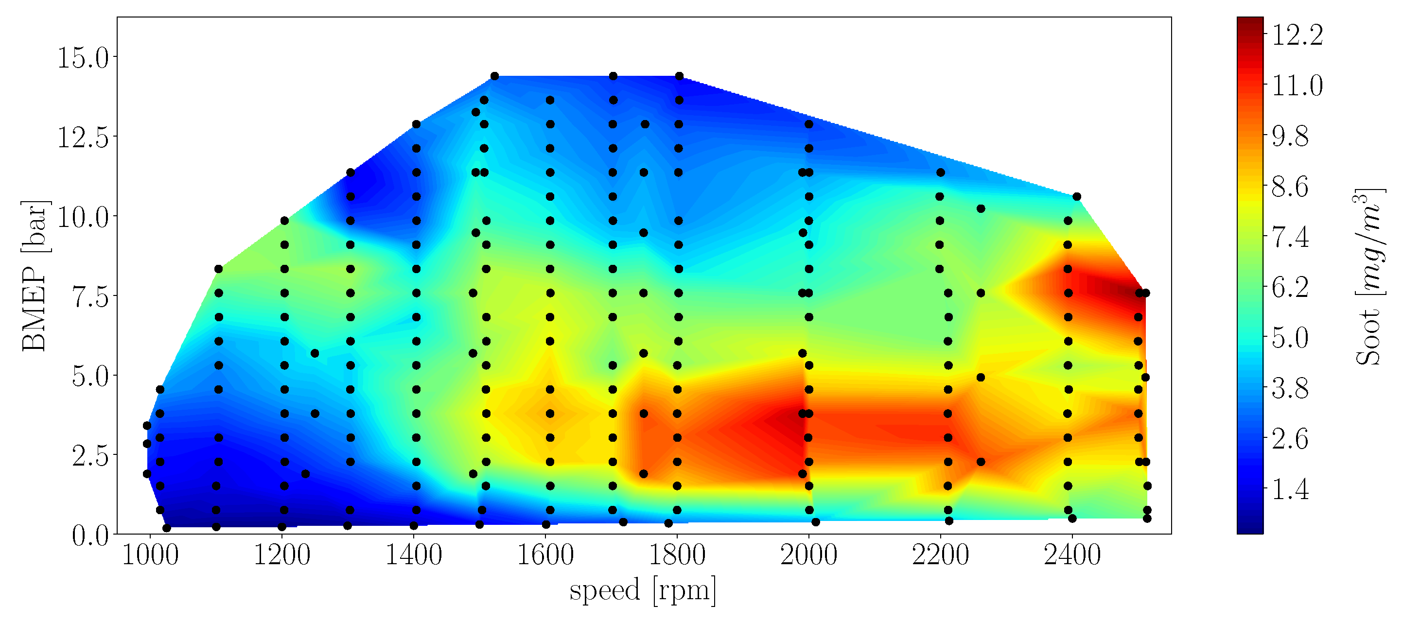
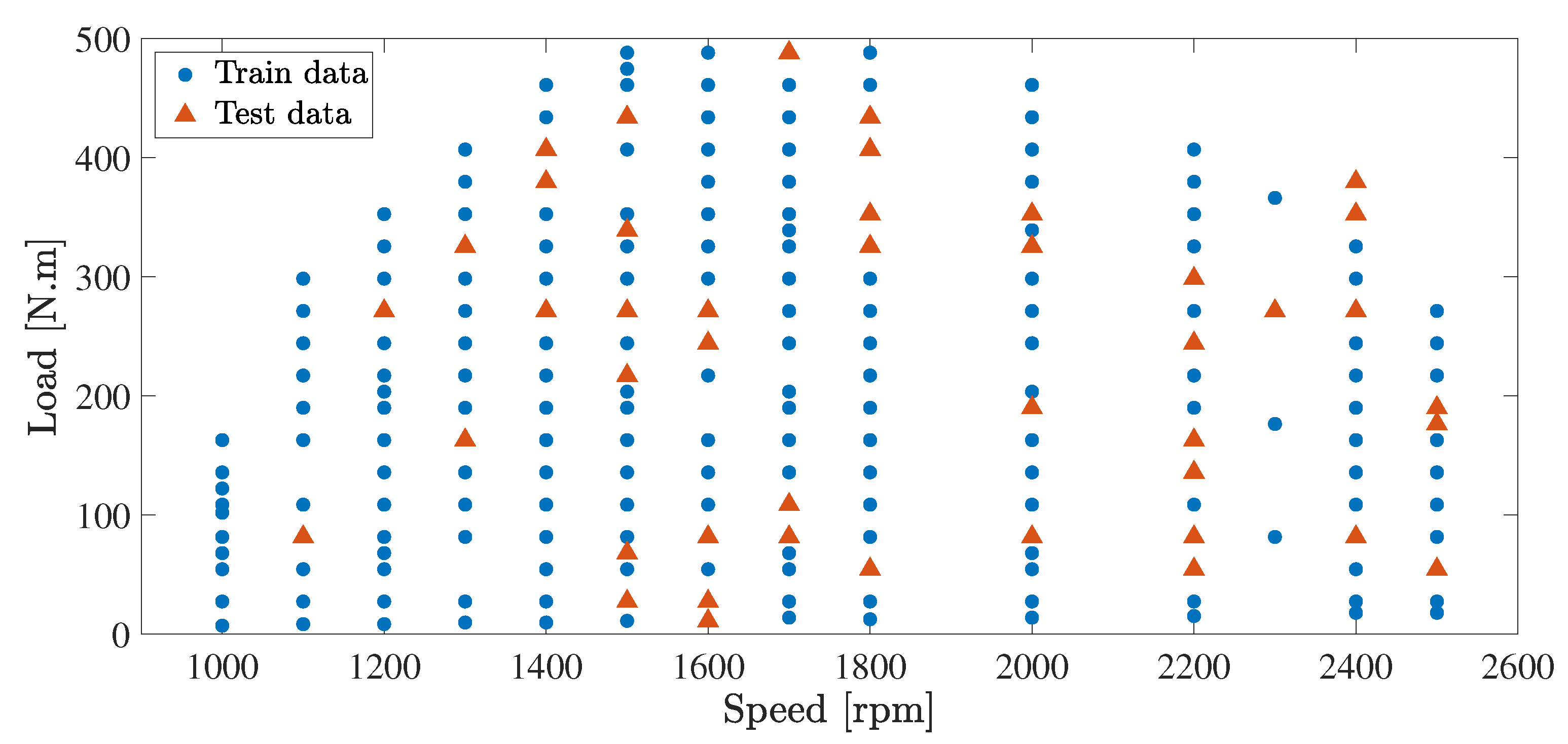
• Although some papers investigated the effects of different parameters on emission production of diesel engines, e.g., effect of fuel properties [30] there is limited published soot emissions data for "full" speed-load maps from medium-duty diesel compression ignition engines in the literature. This is because it is difficult and costly to measure soot emissions accurately and it involves substantial calibration efforts for emission analyzers. In this work, the soot emissions data for full speed-load map of a 4.5 L 4-cylinder diesel engine is measured. This dataset provides a benchmark to test different modeling methods in this study.
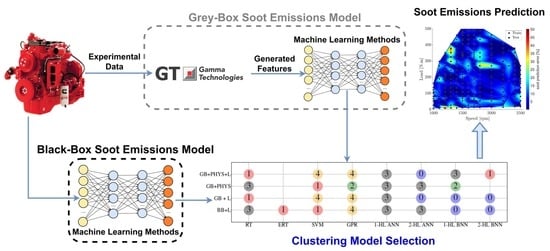
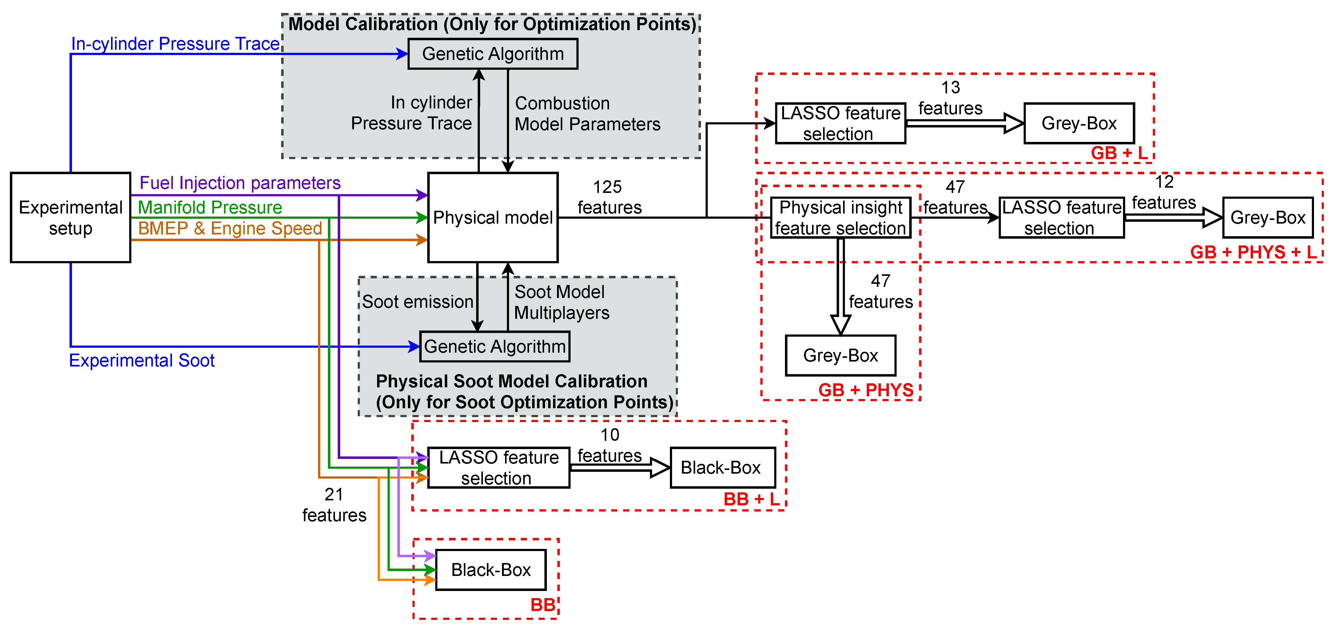
• The performance of ML methods is highly dependent on the input feature set. In emission modeling using ML methods, it is common to mainly use physical knowledge to choose the input feature set. Using physical knowledge has the risk of missing some crucial features due to unknown and misunderstood physical relations. This is especially important in gray-box emission modeling because it generates many features making it difficult to choose a subset based on physical knowledge. In this paper, different input feature sets based on ML feature selection and physical knowledge are investigated to select the optimal input features.
• Previous studies used conventional ML methods such as SVM and ANN and GPR with fixed input feature set for soot emissions modeling. There is a lack of comprehensive studies that investigate different ML methods and feature sets for soot emissions modeling. In this paper, eight different ML methods with five different input feature sets (40 models in total) are used for soot emissions modelling.
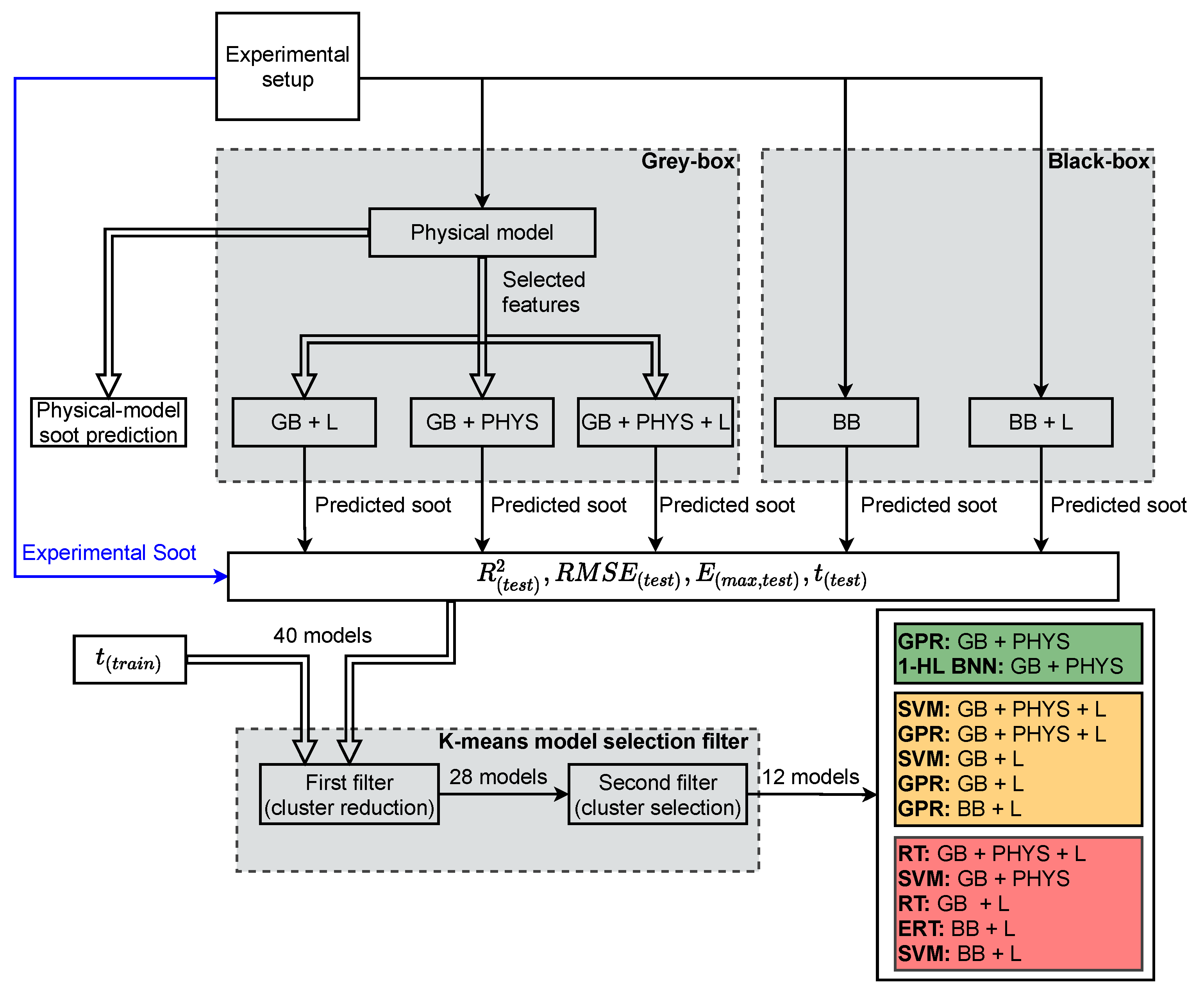
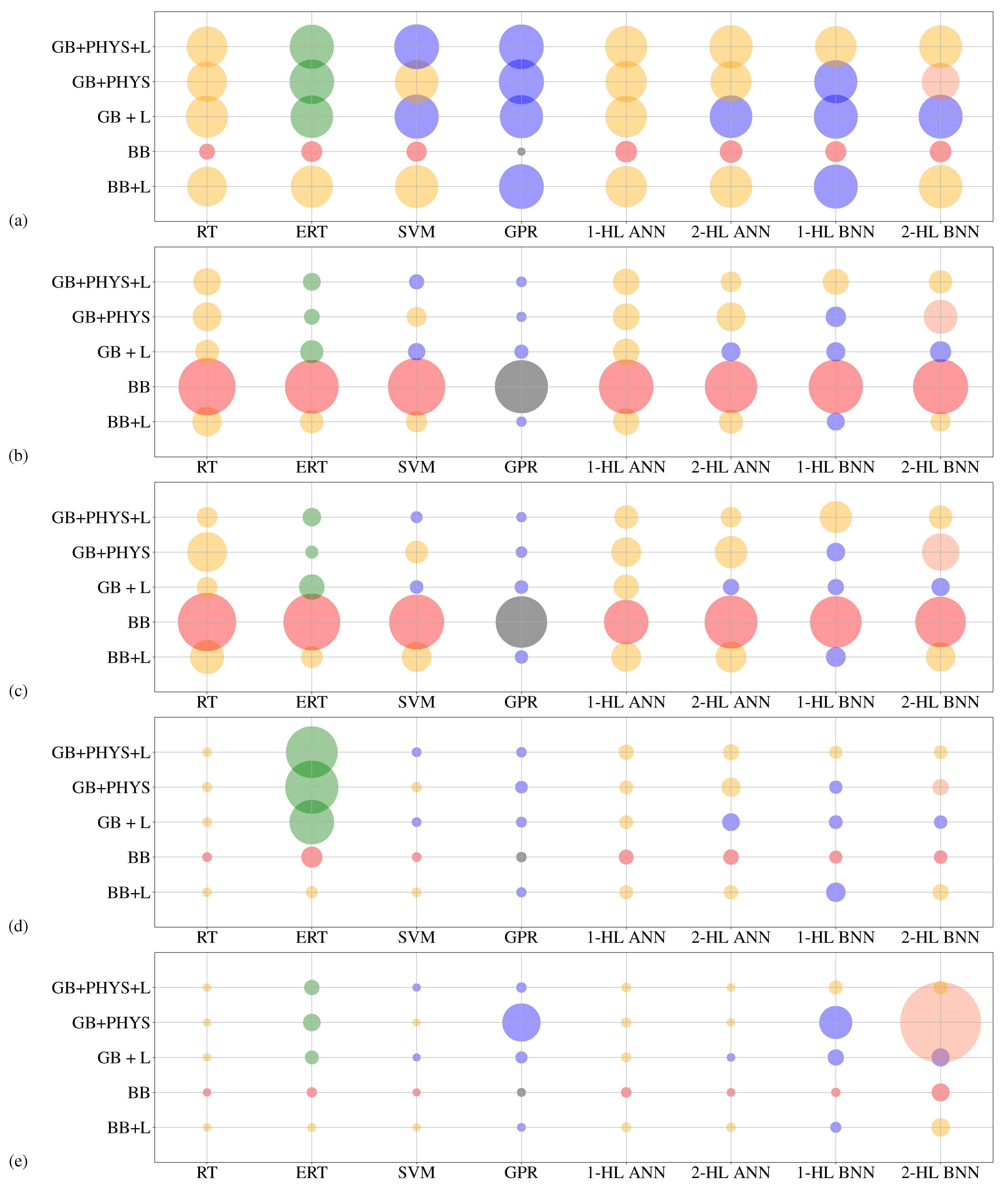
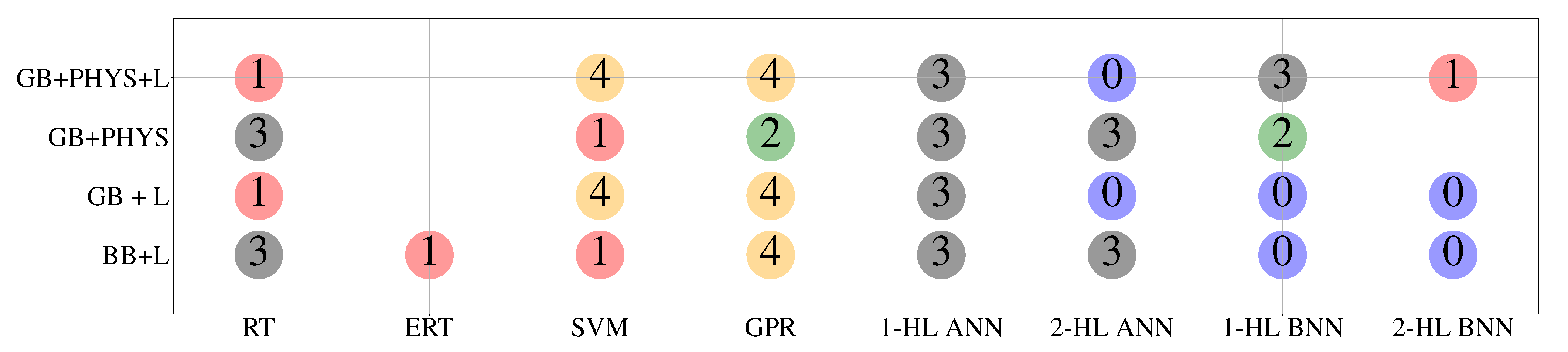
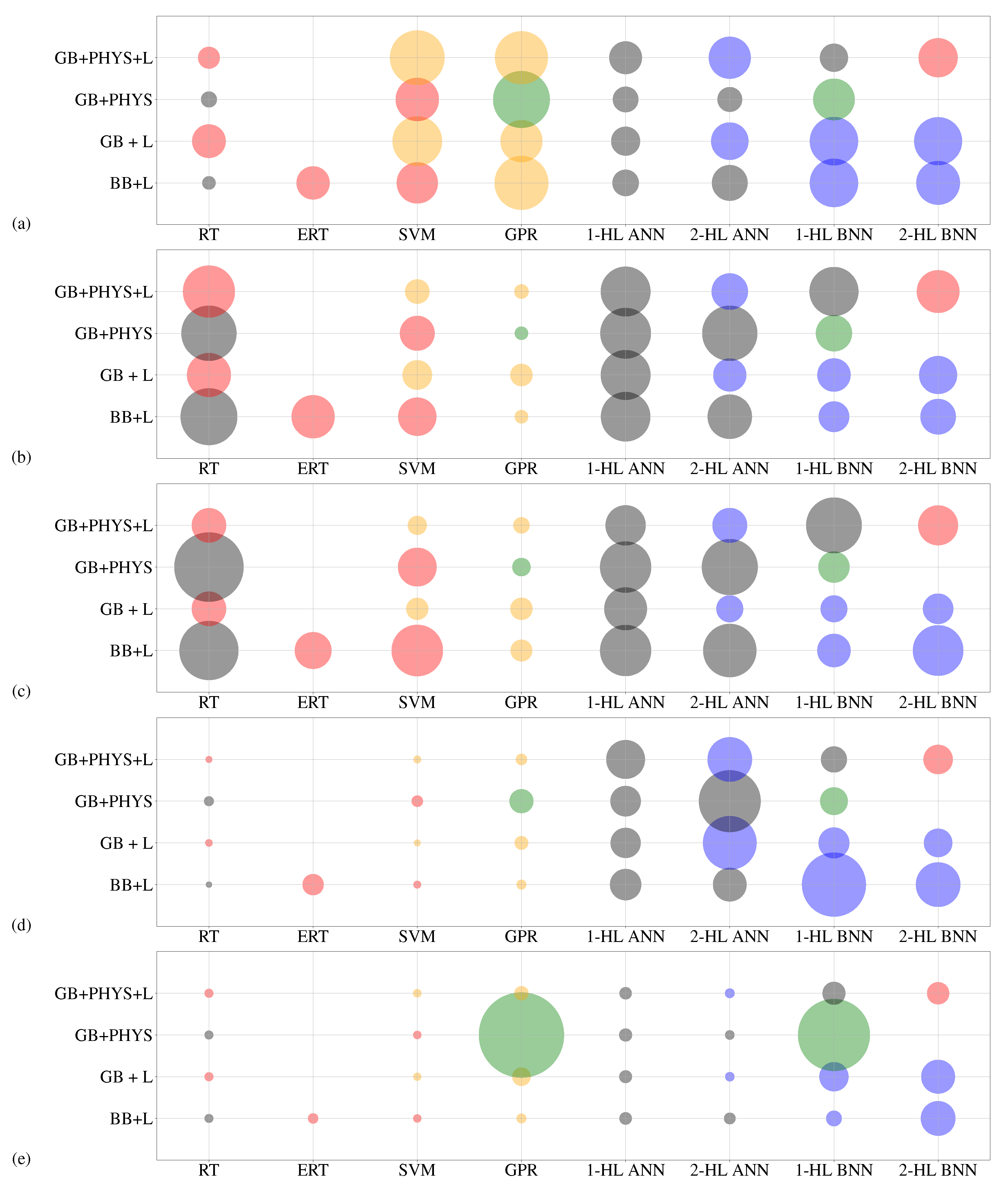
• Post processing methods for analysing the results and method selection have not been used in the previous soot emissions modeling studies. In this paper, a systematic unsupervised ML method is used for analyzing and comparing different engine soot emissions models. Two K-means clustering algorithms that perform as filters are used to select the best soot emissions models. This method could also be used for other engine modeling studies.

The paper is structured in sections. First, the experimental setup and physical model of the engine are described. Second, the black-box and gray-box models are explained. Five different feature sets (2 for the black-box model and 3 for the gray-box model) are used. Third, ML methods that are applied to pre-processing, processing and post processing are described briefly. Fourth, results of different methods and feature sets are compared and analysed in terms of accuracy, complexity, and timing by using a K-means clustering algorithm. Finally, conclusions are described in the last section.

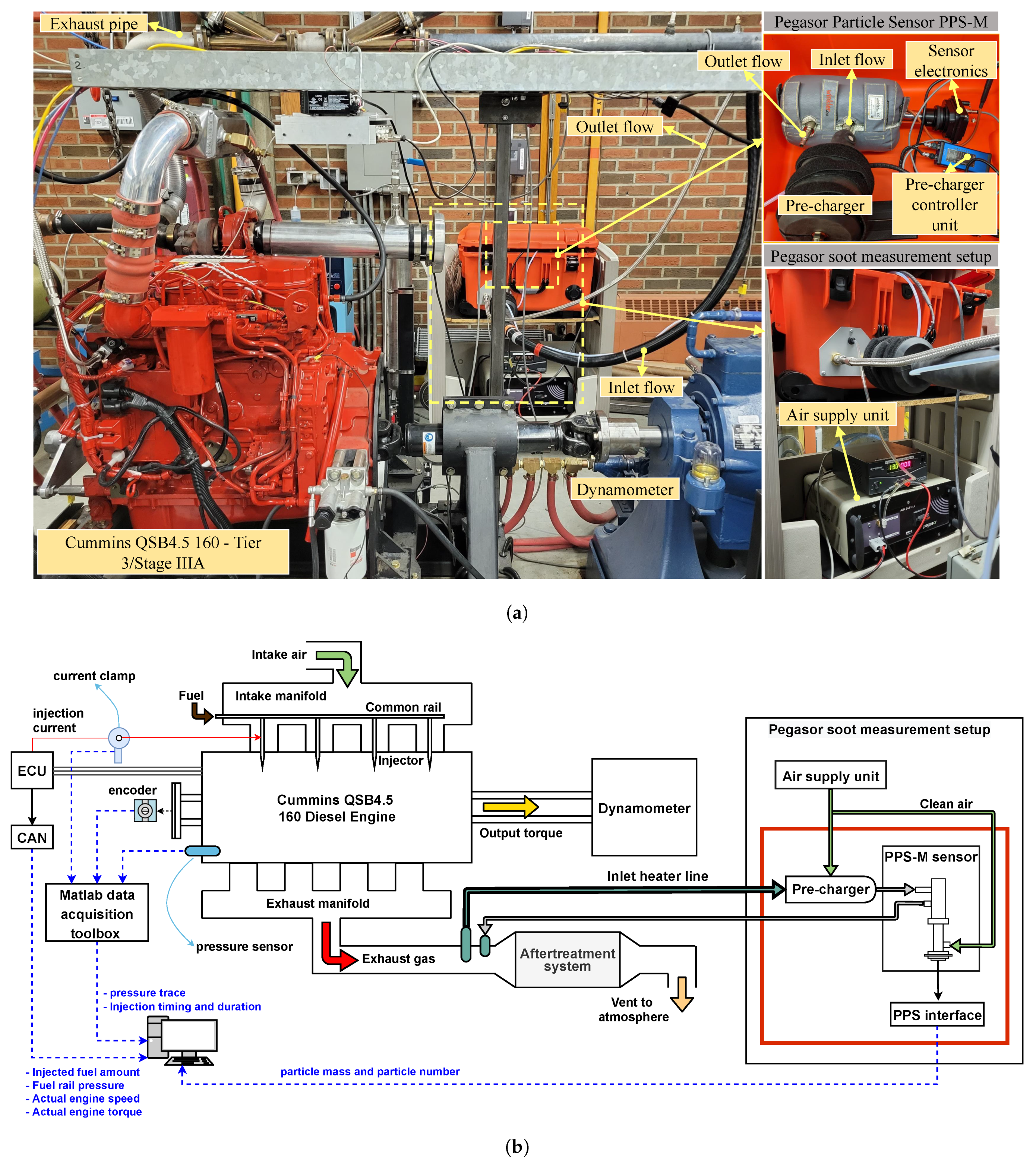
2. Experimental Setup

In this work, a 4.5-L medium-duty Cummins diesel engine is used to collect soot emissions data. Cummins QSB4.5 160 diesel engine specifications are listed in

Table 1. Engine specifications.

Parameter	Value
Engine type	In-Line, 4-Cylinder
Displacement	4.5 L
Bore × Stroke	102 mm × 120 mm
Peak torque	624 N.m @ 1500 rpm
Peak power	123 kW @ 2000 rpm
Aspiration	Turbocharged and Charge Air Cooled
Certification Level	Tier 3/Stage IIIA

. This engine is tested in the University of Alberta internal combustion engine lab, and experimental setup and the schematics of experimental setup for soot emissions data collection are shown in Figure 1. In this setup, intake air pressure, engine speed, load, injected fuel amount, and fuel rail pressure are recorded from the engine ECU. To record these data, the Cummins INLINE6 interface is used to connect ECU to the computer, and INSITE Pro Cummins is used to record and monitor data. A Kistler piezoelectric pressure sensor and Pico current clamp are used to measure the in-cylinder pressure and the injector command signal.

To measure soot emissions, a Pegasor Particle Sensor (PPS-M) is used. The schematic of the soot measurement setup is also shown in Figure 1b where engine-out exhaust gas flows through an inlet heater line to the pre-charger. The pre-charger is used to avoid any charge-related problem in soot measurement [31]. The pre-charger is essential to the accuracy of soot measurement as in recent emission technology, microscopic particles in the exhaust may be strongly charged. The Pegasor Pre-Charger is a self-heated, non-radioactive, negative diffusion charger. Using an integrated ion trap, Pegasor can eliminate ions and small charged particles from the sample line gas and it charges larger particles into a known negative charge state. The sampling rate of PPS-M is 100 Hz with 100 dB Sensor to Noise Ratio (SNR). This sensor detects particle sizes in the range of $[0.001,290][\mathrm{mg}/{\mathrm{m}}^3]$. The main PPS-M sensor’s specifications are listed in

Table 2. The PPS-M sensor specifications.

Parameter	Value
Sensor temperature	200 °C
Extracted sample temperature	−40 up to 850 °C
Dilution	No need
Time response	0.2 s
Measured particle size range	10 nm and up
Trap voltage	60 V (10 nm lower cut) 400 V (23 nm lower cut, default) 2 kV (90 nm lower cut)
Particle number range	300 up to 109 $1/{\mathrm{cm}}^3$
Particle mass range	10−3 up to 300 $\mathrm{mg}/{\mathrm{m}}^3$
Sample pressure	−20 kPa to +100 kPa
Clean air/Nitrogen supply	10 LPM @ 0.15 MPa
Operating voltage	24 V
Power consumption	6 W

.

The diesel engine was tested for 219 engine steady state operating conditions over the full range of engine speeds and loads. Figure 2 shows the color map of raw soot emissions data with respect to engine speed (x-axis) and load (y-axis), where black dots represent experimental points. Since this engine is designed for stationary applications, it has limited operating conditions. Therefore, 219 data points in Figure 2 covers most of the possible operating conditions. It is worth mentioning that for highway truck application, due to various driving cycles, 220 data points might not be sufficient as in the literature for such an application, more than 900 data points were used [26].

To analyze the main features of the diesel engine that play an important role both in soot emissions modeling, the histogram of them are plotted in Figure 3. This diesel engine has three injection pulses, and the third injection is active in 39% of our experimentally collected data based on Figure 3b. Start and duration of all pulse of injections along with total injected fuel in each cycle are shown in Figure 3a–d. Another main fuel path feature that affects soot emissions modeling is common rail pressure as shown in Figure 3e. The majority of data are collected in fuel rail pressure from 700 to 1100 bar. The air path, intake manifold pressure and air-fuel equivalence ration ($\lambda$) are shown in Figure 3f–g. Output torque and engine speed are the other important feature that are shown in Figure 3h–i. According to these histograms, the data collected from experiments successfully cover most of the operating conditions of the engine.

3. Gray-Box and Black-Box Models

The physical model, black-box, and gray-box are described in this section. The first step toward developing physical and gray-box models was developing and parameterizing the GT-Power physics-based model. GT power is a commercial software for modeling combustion engines. Physical modeling of the diesel engine is carried out using the GT power software, which contains several chemical and physical sub-models that simulate complex combustion processes. DIpulse is used as the combustion model since it can be applied to multi-injection diesel combustion engine.

The Hiroyasu model [32] is used as the physical soot model. The model is calibrated by using 8% of the experimental data. The calibration process uses Genetic Algorithm (GA) NSGA-III [33] for multi-objective Pareto optimization as the search algorithm. GA is the optimal choice for problems with different levels of complexity, because of its ability to explore a broad design space [33]. The two key inputs for GA are the population size and the number of generations. Here, two different GAs are used for combustion model calibration and soot model calibration. The population size is 16 for both algorithms but the number of generations for combustion model calibration and soot model calibration are 16 and 10, respectively, due to combustion model complexity and including more factors compared to the soot model. Figure 4 schematically shows how the soot model and combustion model multipliers are calculated using the GA-based algorithm. The GAs, based on the results obtained, took into account experimental results of soot emissions and in-cylinder pressure traces for some optimization points. The multipliers for combustion model are: Entertainment Rate Multiplier, Ignition Delay Multiplier, Premixed Combustion Rate Multiplier, and Diffusion Combustion Rate Multiplier. There are also these two multipliers in the soot model: the soot formation multiplier and the soot burn-up multiplier. The GAs minimize the deviation between the experimental and simulation in-cylinder pressure trace and soot emissions values to calculate the optimal multipliers. In this case, the calibration process for soot emissions and in-cylinder pressure trace was done separately using two different GAs.

The number of injection pulses and injection timing are important control inputs that affect soot emissions production in diesel engines [34]. There are three main pulses in the Cummins diesel engine injection system in this work; Pulse I is pre-injection, Pulse II is the main injection, and Pulse III is post-injection which only occur for limited load areas. Post injection plays a crucial rule in lowering soot emissions production by increasing the soot emissions burn rate [35].

The in-cylinder pressure trace for different load and speed conditions are shown as a function of crank angle (CAD) in Figure 5. Case I (136 $\left[\mathrm{N}.\mathrm{m}\right]$ in 1200 $\left[\mathrm{rpm}\right]$), case IV (271 $\left[\mathrm{N}.\mathrm{m}\right]$ in 1800 $\left[\mathrm{rpm}\right]$) and case VI (353 $\left[\mathrm{N}.\mathrm{m}\right]$ in 2400 $\left[\mathrm{rpm}\right]$) are selected from optimization points for model calibration (refer to Figure 4) while other cases are not used for calibration. The validation result for crank angle position where 50% of the heat is released (CA50), NOx, intake manifold pressure and maximum in-cylinder pressure are shown in Figure 6. The average error for CA50 and maximum in-cylinder pressure are about 2 CAD and 6% respectively, demonstrating the physical model’s reliability.

The process of selecting important features out of feature set is called feature selection (FS). FS reduces the size of input feature set which results in improving ML method performance. FS process is depicted schematically in Figure 4. A total of five feature sets are used in this study to simulate soot emissions. For FS in this work, a combination of physical insight and LASSO feature selection technique is used. For physical insight feature selection, the most significant features are selected based on an expert prior knowledge while LASSO feature selection offers more systematic way for feature selection regardless of prior knowledge of system.

Two black-box feature sets (contain only experimental data) that are used are, without any feature selection method (BB), and black-box + LASSO (BB + L). The gray-box features sets are: GB + PHYS, GB + L and GB + PHYS + L. In GB + PHYS, data-driven features are chosen solely based on physical insight into soot oxidation and formation processes. With GB + L, the LASSO feature selection method selects the parameters. Finally, GB + PHYS + L first uses physical insight to select the most important features, then the LASSO feature selection method is applied to select the final features. The number of features for the five different methods and steps are summarised in Figure 4.

A schematic representation of black-box and gray-box soot modeling is shown in Figure 7. As seen, the experimental injection timing is used for the virtual engine. The gray-box and black-box model inputs are similar to those shown in Figure 4, including injection properties (total mass of injected fuel, start of injection (SOI), fuel rail pressure), intake manifold pressure, BMEP, and engine speed. The K-means clustering algorithm is used for selecting the most suitable models and feature sets based on errors and timing (testing and training times). Two K-means clustering algorithms are applied (the first filter and the second filter). The first filter eliminates feature sets and models with low accuracy and slow training time and prediction time, whereas the second filter selects the best ML method along with feature sets in terms of accuracy and training and prediction cost for different applications. Finally, 12 soot models are chosen in total, which will be explained further in the Results and discussion section below.

4. Machine Learning Methods

ML algorithms are used in all three sections of this study including pre-processing, modeling, and post-processing.

4.1. Pre-Processing: Feature Selection

For finding the most effective soot prediction parameters, LASSO feature selection algorithm is employed for both black-box and gray-box models. LASSO is a regression method that performs feature selection and regularization to improve the model’s prediction accuracy. In LASSO regression, the predicted output is ${\widehat{y}}_i={\theta }^T{x}_i$ where $\theta$ is model’s coefficient that is calculated by minimizing the following cost function

$$J\left(\theta \right)=\frac{1}{m}\sum _{i=1}^m{(y_i-{\widehat{y}}_i)}^2+\lambda \sum _{i=1}^m\left|{\theta }_i\right|$$

(1)

where m is the number of training data points, ${\sum }_{i=1}^m\left|{\theta }_i\right|$ is the $L_1$ regularization and $\lambda$ is regularization variable. Adding $L_1$ regularization leads to driving the weights down to exactly zero (produces sparsity in the solution) and results in performing a systematic feature selection [36]. This sparsity depends on $\lambda$, which is calculated in the cross-validation process in the current study.

4.2. Regression Models

The five well-known supervised learning regression algorithms are employed: Regression Trees (RT), Ensemble of the Regression Trees (ERT), Gaussian Process Regression (GPR), Support Vector Machine (SVM), and Neural Network (NN). These are used to train both the black and gray-box soot models.

A data-driven regression model can be generalized to fitting a parameterized model, $\widehat{y}=h_{\theta }\left(x_i\right)$, for given training set ${\mathcal{D}}_{train}=(x_i,y_i)$ such that $\widehat{y}$ converges to $y_i$ subject to given constrains. In this problem, $x_i$ is input feature, $y_i$ is the measured output, and $\theta$ is the parameters set. The parameters set can be calculated by solving following optimization problem

$$\begin{array}{cc}\hfill \underset{\theta }{min}& J\left(\theta \right)\hfill \\ \hfill \mathrm{s}.\mathrm{t}.& \varphi \left(\theta \right)\hfill \end{array}$$

(2)

where $\varphi \left(\theta \right)$ is constraints function and $J\left(\mathsf{\Theta }\right)$ is a cost function which is defined as

$$J\left(\mathsf{\Theta }\right)=\overline{J}\left(\mathsf{\Theta }\right)+\lambda L\left(\mathsf{\Theta }\right)$$

(3)

where $\overline{J}\left(\mathsf{\Theta }\right)$ is defined based on error $e_i\left(\mathsf{\Theta }\right)=h_{\theta }\left(x_i\right)-y_i$ to minimize prediction error while regularization term, $L\left(\mathsf{\Theta }\right)$, is added to regulate parameters, $\mathsf{\Theta }$. In general, $L\left(\mathsf{\Theta }\right)$ is $L_1$ or $L_2$ loss function for regularization purpose. For LASSO regression, $L_1$ loss function is used while in other regression methods such as Ridge, SVM, and ANN $L_2$ loss function is used. $L_2$ loss function is defined as

$$L_2\left(\mathsf{\Theta }\right)=\sum _{i=1}^m{\left(\theta \right)}^2$$

(4)

The regulatory parameter or penalized variable, $\lambda$, produces a trade-off between the smoothness of the model and the training error tolerance minimization [36].

4.2.1. K-Fold Cross Validation

K-fold cross-validation algorithm is used to avoid overfitting of models during training. K-fold cross-validation first rearranges the dataset randomly and then divides the dataset into k groups. In this study, 5-fold validation is used for all ML methods. In each iteration, the K-fold algorithm chooses one group as a fold, trains a model on the rest of the groups (out of the fold), and assess it on the fold set [37].

4.2.2. Hyperparameters Optimization

Hyperparameters of ML methods such as tolerated error (defined inside constrain function $\varphi \left(\theta \right)$), regularization parameter ($\lambda$), optimization iteration stop criteria in optimization problem of Equation (2) play an important role to decrease modeling error and to increase model reliability. If an ML algorithm such as ${\mathrm{A}}_{\mathsf{\Lambda }}$ has N hyperparameters such as $\mathsf{\Lambda }={\lambda }_1,{\lambda }_2,...,{\lambda }_N$, the optimum hyperparameters can be found by solving following optimization problem [38]

$${\mathsf{\Lambda }}^{*}=\arg \underset{\mathsf{\Lambda }}{min}V(h_{\theta }\left(x_i\right),{\mathcal{D}}_{train},{\mathcal{D}}_{valid})$$

(5)

where $V(h_{\theta }\left(x_i\right),{\mathcal{D}}_{train},{\mathcal{D}}_{valid})$ measures performance of a model for given training and validation set, ${\mathcal{D}}_{training}$ and ${\mathcal{D}}_{valid}$ based on algorithm ${\mathrm{A}}_{\mathsf{\Lambda }}$.

In this work, Bayesian optimization [39] is used for RT, SVM, and ERT models hyperparameters optimization while grid search [36] method is used for NN-based models such as ANN and BNN.

For the Bayesian optimization to tune hyperparameters, the evaluation used in Equation (5) is

$$V\left(\lambda \right)=\frac{1}{n}\sum _{i=1}^m{(\widehat{y_i}-y_i)}^2$$

(6)

where ${\mathrm{A}}_{\mathsf{\Lambda }}\in \{\mathrm{RT},\mathrm{ERT},\mathrm{SVM}\}$ and m is size of training set. The model is trained based on training ${\mathcal{D}}_{train}$ and cross-validated on ${\mathcal{D}}_{valid}$ in the inner loop of this optimization. Then, $V\left(\lambda \right)$ is calculated using both training and cross-validation sets.

To evaluate all possible hyperparameter combinations in NN-based methods, grid search is often used [26]. A search along the space of hyperparameters learning with high probability is tried in Bayesian optimization while in grid search, all the possible hyperparameters combinations within a given range are tried. In this study, all combination of layer $L\in \{1,2\}$ (shallow network) and neurons $s_l\in (1,40)$ are considered where L and $s_l$ are number of layers and number of neurons in $l^{th}$ layer. The layers and neuron’s upper limit are set to 2 and 40, respectively, since the limited number of training data means a deeper network should be avoided.

4.2.3. Regression Tree (RT)

Regression Tree (RT) is a modeling method with an iterative process of splitting the data into branches where the main algorithm to train RT is Classification and Regression Trees (CART) [40]. In a regression tree, the data are divided into different classes similar to classification problem with only difference is that each class is assigned to a specific value. RT divides data to k classes based on threshold, $t_k$, based on following cost function

$$J\left(\theta \right)=\frac{m_{left}}{m}{\mathrm{MSE}}_{left}+\frac{m_{right}}{m}{\mathrm{MSE}}_{right}$$

(7)

where Mean Squared Error (MSE) is defined as

$$\mathrm{MSE}\left(\theta \right)=\frac{1}{m}\sum _{i=1}^m{(y_i-{\widehat{y}}_i)}^2$$

(8)

where $\widehat{y}=\frac{1}{m_{node}}{\sum }_{i\in \mathrm{node}}y\left(i\right)$ and $m_{left}$ and $m_{right}$ are left and right branches of the tree. In this method, both k and $t_k$ are considered as model weights and integrated in $\theta$. To avoid overfitting, a minimum number of samples required at a leaf node (Minimum Samples Leaf (MSL)) is added to the CART algorithm as a regularization parameter. The maximum depth of tree that integrated in $\varphi \left(\theta \right)$ is another regularisation parameter [36].

4.2.4. Ensemble of Regression Trees (ERT)

ERT is constructed using several decision trees. Three primary hyperparameters to tune ERT are aggregation methods, number of learners, and MSL. In ensemble learning, Bootstrap aggregation (Bagging) and hypothesis boosting (Boosting) are two standard aggregation methods. In bagging, the training algorithm is the same for every predictor, while the training set is a random subset of the training set, i.e., several RT are trained based on different random subsets of the training set. The well-known example of using bagging method is Random Forest. In boosting, a sequential architecture of several weak learners is aggregated, i.e., series of RTs are trained based on the same training data and layers of RT connected through a series architecture [36]. In this study, Bayesian optimization is used to tune the ERT hyperparameters including number of learners (number of RT in ERT), MSL, and aggregating method (boosting/bagging).

4.2.5. Support Vector Machine (SVM)

Support Vector Machine (SVM) is an ML method to find a correlation between input-output by solving a convex quadratic programming problem. The cost function of SVM can be defined as

$$J\left(\theta \right)=\frac{1}{2}\sum _{i=1}^m{\theta }_i^2+C\sum _{i=1}^m({\zeta }_i^{+}+{\zeta }_i^{-})$$

(9)

where ${\zeta }_i^{-}$ and ${\zeta }_i^{+}$, are so-called slack variables and perform as penalty variables to tackle a possible infeasibility of an optimization problem. C includes regulatory parameters. Equation (9) follows the original cost function defined in [41] and equals to $1/\lambda$ [36]. Thus, SVM optimization equation can be rewritten as

$$J\left(\theta \right)=\frac{\lambda }{2}\sum _{i=1}^m{\theta }_i^2+\sum _{i=1}^m({\zeta }_i^{+}+{\zeta }_i^{-})$$

(10)

The constraint function, $\varphi \left(\theta \right)$, of SVM in Equation (2) is

$$\varphi \left(\theta \right)=\left\{\begin{array}{c}{y}_i-h_{\theta }\left(x_i\right)\le ϵ+{\zeta }_i^{+}\hfill \\ h_{\theta }\left(x_i\right)-y_i\le ϵ+{\zeta }_i^{-}\hfill \\ {\zeta }_i^{-},{\zeta }_i^{+}\ge 0\hfill \end{array}\right.$$

(11)

where $ϵ$ is the maximum tolerable deviation for all training data [8,42,43]. In SVM, instead of training data in $\widehat{y}=h_{\theta }\left(x_i\right)$, a function of training data, so-called kernel function can be replaced, $\widehat{y}=h_{\theta }\left(\mathsf{\Gamma }\left(x_i\right)\right)$. This method is called SVM kernels trick and adding the kernel does not affect the cost function other than using higher dimension feature set instead of $x_i$ in $\widehat{y}$. Different kernels such as linear, polynomial, and Gaussian RBF kernels can be considered in optimization. These kernels are defined as

$$K(x_i,x_j)=\left\{\begin{array}{c}{x_i}^T{x}_j\mathrm{Linear}\hfill \\ {({x_i}^T{x}_j+c)}^n\mathrm{Polynomial}\hfill \\ exp(-\gamma ||x_i-x_j|{|}_2^2)\mathrm{Gaussian}\mathrm{RBF}\hfill \end{array}\right.$$

(12)

where n and $\gamma$ are degree of polynomial and scale of RBF kernel, respectively [44]. In this study, optimal kernel type including kernel parameters, i.e., scale and degree of freedom, as well as $\lambda$ and $ϵ$ are found using Bayesian optimization.

4.2.6. Gaussian Process Regression (GPR)

GPR is a nonparametric and Bayesian-based approach that has superior performance with small data sets and can provide an uncertainty measure on the predictions [45]. The main advantage of GPR is probabilistic prediction. Unlike other supervised ML methods, GPR infers a probability distribution over all possible ML model parameter values. The GPR cost function is defined based on negative log marginal likelihood as

$$J\left(\theta \right)=-log\left(p\right(\theta |y,X))$$

(13)

where $p\left(\theta \right|y,X)$ is posterior distribution (i.e., a likelihood function of $\theta$ given X and y) that is defined based on Bayes’ Rule as

$$p\left(\theta \right|y,X)=\frac{p\left(y\right|X,\theta \left)p\right(\theta )}{p\left(y\right|X)}$$

(14)

$p\left(y\right|X,\theta )$ is a likelihood function of y given X and $\theta$, and $P\left(y\right|X)$ is marginal likelihood function of y given X [45]. Different covariance kernel functions are considered in this study, such as Exponential Kernel, Matern, and Quadratic Kernel with different options. Here, two standard kernels for GPR method including Rational Quadratic kernel function and Matérn kernel function are used. Rational Quadratic kernel function defines as

$$K(x_i,x_j|\theta )={\sigma }_l^2{(1+\frac{r^2}{2\alpha {\sigma }_l^2})}^{-\alpha }$$

(15)

and general Matérn kernel function defines as

$$K_{p+1/2}(x_i,x_j)={\sigma }_f^{2}exp(-\frac{\sqrt{2p+1}r}{{\sigma }_l})\frac{p!}{\left(2p\right)!}\sum _{i=1}^p\frac{(p+i)!}{i!(p-i)!}{(\frac{2\sqrt{2p+1}r}{{\sigma }_l})}^{p-i}$$

(16)

where r is the Euclidean distance between $x_i$ and $x_j$ ($r=\sqrt{{(x_i-x_j)}^T(x_i-x_j)}$), ${\sigma }_l$ is characteristic length scale, ${\sigma }_f$ is signal standard deviation, and $\alpha$ is a positive-valued scale-mixture parameter [45]. In Equation (17), usual value for p is $p=0$ (Matérn 1/2 $K_{1/2}(x_i,x_j)$), $p=1$ (Matérn 3/2 $K_{3/2}(x_i,x_j)$), and $p=2$ (Matérn 5/2 $K_{5/2}(x_i,x_j)$). The Beysian optimization method in this study results using Matérn 5/2 function as a optimum choice for GB + L, GB + PHYS, and GB + PHYS + L which defines as

$$K_{5/2}(x_i,x_j)={\sigma }_f^2(1+\frac{\sqrt{5}r}{{\sigma }_l}+\frac{5r^2}{3{\sigma }_l^2})exp(-\frac{\sqrt{5}r}{{\sigma }_l})$$

(17)

4.2.7. Neural Network (NN)

In general, Neural Network (NN) is a set of algorithms to model phenomena by mimicking human brain operation behavior. NN contains three main layers: the input layer, hidden layer (HL), and output layer network [46]. As we have a small amount of data, only shallow neural networks with only 1 or 2 hidden layers are considered in this study which are denoted as ANN. Similar to previous ML methods, the cost function of an NN method can be written following Equation (2) notation as

$$J\left(\theta \right)=\sum _{i=1}^m(h_{\theta }\left(x_i\right)-y_i)+\frac{\lambda }{2}\sum _{k=1}^{K-1}\sum _{i=1}^{s_k}\sum _{j=1}^{s_{k+1}}{({\theta }_{j,i}^{\left(k\right)})}^2$$

(18)

where K and $s_k$, and m are number of total layers (input + output + hidden layer), number of neurons in $k^{th}$ layer, and size of the training set, respectively. The first term in this equation is used to minimize modeling error while $L_2$ loss function is used for regulization. As input neurons and output neurons are set by input and output layers, only hidden layer number and neuron size are found by using grid search, i.e., $(L_{HL}=K-2)$ and the number of neurons ($s_2$ and $s_3$) in the HL.

Bayesian-based NN, denoted as BNN, is referring to extending ANN with Bayesian inference. Unlike ANN which model’s weights are assigned as a single value, in BNN, weights are considered a probability distribution. These probability distributions of network weights are used to estimate the uncertainty in weights and predictions [47]. All ANN and BNN configuration combinations are evaluated in this optimization method, and the best model is obtained based on cross-validation data.

The summary of developed models, along with hyperparameters optimization method and optimized parameters, are listed in

Table 3. Training and optimization of ML-based model hyperparameters. In this table MSL is minimum samples leaf for regression tree and ensembles trees methods, $\lambda$ is the regularization parameter and $ϵ$ is the maximum tolerable deviation for support vector machione method, and ${\sigma }_l$ is the length scale of Gaussian process regression method.

Method	Opt. Method	Opt. Hyperparameters	Model Type	Opt. Model Configuration
RT	Bayesian	Min samples leaf (MSL)	BB	MSL = 13
			BB + L	MSL = 1
			GB + L	MSL = 5
			GB + PHYS	MSL = 5
			GB + PHYS + L	MSL = 5
ERT	Bayesian	Ensemble method, min samples leaf, and number of learners	BB	Boosting, 75 Learners, and MSL = 2
			BB + L	Boosting, 28 Learners, and MSL = 4
			GB + L	Boosting, 35 Learners, and MSL = 5
			GB + PHYS	Boosting, 488 Learners, and MSL = 47
			GB + PHYS + L	Boosting, 487 Learners, and MSL = 2
SVM	Bayesian	Kernel function $\lambda$ and $ϵ$	BB	Cubic, $\lambda =0.96$, $ϵ=0.010$
			BB + L	Quadratic, $\lambda =0.77$, $ϵ=0.330$
			GB + L	Gaussian, $\lambda =9.59$, $ϵ=0.004$
			GB + PHYS	Quadratic, $\lambda =3.49$, $ϵ=0.003$
			GB + PHYS + L	Cube, $\lambda =5.79$, $ϵ=0.009$
GPR	Bayesian	Kernel function, initial value for the noise standard deviation ($\sigma$)	BB	Rational quadratic, $\sigma =12.68$
			BB + L	Rational quadratic, $\sigma =0.0005$
			GB + L	Matérn 5/2, $\sigma =0.0001$
			GB + PHYS	Matérn 5/2, $\sigma =0.0001$
			GB + PHYS + L	Matérn 5/2, $\sigma =2.996$
1-HL ANN	Grid search	Number of neurons in each layer	BB	Network conf.: [25]
			BB + L	Network conf.: [19]
			GB + L	Network conf.: [4]
			GB + PHYS	Network conf.: [4]
			GB + PHYS + L	Network conf.: [19]
2-HL ANN	Grid search	Number of neurons in each layer	BB	Network conf.: [7, 25]
			BB + L	Network conf.: [25, 31]
			GB + L	Network conf.: [4, 13]
			GB + PHYS	Network conf.: [7,13]
			GB + PHYS + L	Network conf.: [16, 19]
1-HL BNN	Grid search	Number of neurons in each layer	BB	Network conf.: [7]
			BB + L	Network conf.: [31]
			GB + L	Network conf.: [31]
			GB + PHYS	Network conf.: [13]
			GB + PHYS + L	Network conf.: [25]
2-HL BNN	Grid search	Number of neurons in each layer	BB	Network conf.: [7, 28]
			BB + L	Network conf.: [16, 13]
			GB + L	Network conf.: [10, 22]
			GB + PHYS	Network conf.: [22, 22]
			GB + PHYS + L	Network conf.: [10, 19]

.

4.3. Post-Processing: Model Selection

The K-means clustering algorithm, an unsupervised ML method, is used for analysing the results and selecting the best feature sets and methods for different applications. K-means algorithm divides data into n clusters with equal variance. To do this the K-means algorithm tries to divide this data into M disjoint clusters, then minimizes the within-cluster sum-of-squares or inertia, which is the sum of squared Euclidean distance between cluster members and cluster center

$$E(m_1,...,m_M)=\sum _{i=1}^N\sum _{k=1}^{M}I(x_i\in C_k)\left|\right|x_i-m_k{\left|\right|}^2$$

(19)

where $m_k$ is the center of cluster k. If $x_i\in C_k$, I($x_i\in C_k$) = 1; otherwise, I($x_i\in C_k$) = 0. The algorithm starts with random centers and updates the centers in each iteration until the centers remain unchanged, which is a local optimum point. In order to find out the optimum number of clusters for a data set, the elbow method could be used. In this method, inertia is plotted as a function of the number of clusters. The elbow of this curve shows the optimum number of clusters. All these models are evaluated for the test set in Section 5, and results will be discussed.

5. Results and Discussion

The engine experimental data including 80% (175 points) of the data points are used for training ${\mathcal{D}}_{train}$, and 20% of the data points are used for testing ${\mathcal{D}}_{test}$ (44 points). Figure 8 shows the distribution of the test and training data. The K-fold validation method with five folds ($k=5$) is also included in training ${\mathcal{D}}_{valid}$. Testing data ${\mathcal{D}}_{test}$ is used only for the final evaluation of the model.

Table 3 and

Table 4. ML-based data-driven soot models comparison. BB, L, GB, and PHYS stand for black-box, LASSO, grey-box, and physical insight, respectively.

Model	Criteria	RT	ERT	SVM	GPR	1-HL NN	2-HL NN	1-HL BNN	2-HL BNN
BB	${\mathrm{R}}_{\mathrm{train}}^2$	0.85	0.95	0.86	0.87	0.86	0.86	0.88	0.90
	${\mathrm{R}}_{\mathrm{test}}^2$	0.41	0.51	0.50	0.27	0.52	0.54	0.51	0.52
	${\mathrm{RMSE}}_{\mathrm{train}}[\mathrm{mg}/{\mathrm{m}}^3]$	1.41	0.90	1.39	1.35	1.44	1.38	1.27	1.21
	${\mathrm{RMSE}}_{\mathrm{test}}[\mathrm{mg}/{\mathrm{m}}^3]$	2.52	2.38	2.53	2.35	2.41	2.32	2.39	2.43
	$|{\mathrm{E}}_{\mathrm{test},\max }|[\mathrm{mg}/{\mathrm{m}}^3]$	8.7	8.5	8.2	7.7	6.6	7.9	7.7	7.5
	${\mathrm{t}}_{\mathrm{test}}\left[\mathrm{ms}\right]$	2.23	16.73	2.08	3.11	8.66	9.53	6.47	6.93
	${\mathrm{t}}_{\mathrm{train}}\left[\mathrm{s}\right]$	0.74	3.50	0.40	1.56	3.77	1.11	2.07	14.31
BB + L	${\mathrm{R}}_{\mathrm{train}}^2$	0.98	0.99	0.97	1	0.97	0.98	0.99	0.99
	${\mathrm{R}}_{\mathrm{test}}^2$	0.87	0.91	0.93	0.96	0.90	0.92	0.95	0.94
	${\mathrm{RMSE}}_{\mathrm{train}}[\mathrm{mg}/{\mathrm{m}}^3]$	0.48	0.52	0.66	0.28	0.66	0.63	0.22	0.20
	${\mathrm{RMSE}}_{\mathrm{test}}[\mathrm{mg}/{\mathrm{m}}^3]$	1.33	1.07	0.98	0.51	1.19	1.10	0.83	0.93
	$|{\mathrm{E}}_{\mathrm{test},\max }|[\mathrm{mg}/{\mathrm{m}}^3]$	5.02	3.14	4.37	1.87	4.35	4.53	2.85	4.3
	${\mathrm{t}}_{\mathrm{test}}\left[\mathrm{ms}\right]$	1.94	5.26	2.27	2.73	7.49	8	14.7	10.4
	${\mathrm{t}}_{\mathrm{train}}\left[\mathrm{s}\right]$	0.75	1.57	0.44	1.32	2.80	2.33	4.57	15.13
GB + L	${\mathrm{R}}_{\mathrm{train}}^2$	0.97	0.99	0.98	0.99	0.96	0.96	0.99	0.99
	${\mathrm{R}}_{\mathrm{test}}^2$	0.92	0.93	0.95	0.94	0.90	0.92	0.95	0.95
	${\mathrm{RMSE}}_{\mathrm{train}}[\mathrm{mg}/{\mathrm{m}}^3]$	0.62	0.06	0.48	0.38	0.73	0.72	0.34	0.09
	${\mathrm{RMSE}}_{\mathrm{test}}[\mathrm{mg}/{\mathrm{m}}^3]$	1.09	1.00	0.81	0.67	1.2	0.88	0.88	0.97
	$|{\mathrm{E}}_{\mathrm{test},\max }|[\mathrm{mg}/{\mathrm{m}}^3]$	2.9	3.7	1.9	1.9	3.6	2.3	2.3	2.6
	${\mathrm{t}}_{\mathrm{test}}\left[\mathrm{ms}\right]$	2.21	47.16	2.05	3.59	7.24	12.42	7.39	6.86
	${\mathrm{t}}_{\mathrm{train}}\left[\mathrm{s}\right]$	0.79	8.57	0.37	6.1	2.97	1.04	12.10	14.66
GB + PHYS	${\mathrm{R}}_{\mathrm{train}}^2$	0.98	0.99	0.98	0.99	0.97	0.98	0.99	0.99
	${\mathrm{R}}_{\mathrm{test}}^2$	0.87	0.96	0.94	0.97	0.90	0.89	0.93	0.83
	${\mathrm{RMSE}}_{\mathrm{train}}[\mathrm{mg}/{\mathrm{m}}^3]$	0.54	0.01	0.57	0.13	0.70	0.6	0.07	0.01
	${\mathrm{RMSE}}_{\mathrm{test}}[\mathrm{mg}/{\mathrm{m}}^3]$	1.3	0.74	0.91	0.5	1.2	0.94	1.2	1.06
	$|{\mathrm{E}}_{\mathrm{test},\max }|[\mathrm{mg}/{\mathrm{m}}^3]$	5.88	1.8	3.3	1.58	4.35	4.76	2.67	5.52
	${\mathrm{t}}_{\mathrm{test}}\left[\mathrm{ms}\right]$	2.74	58.19	3.1	5.87	7.3	14.22	6.69	10.63
	${\mathrm{t}}_{\mathrm{train}}\left[\mathrm{s}\right]$	0.75	13.90	0.46	43.24	3.09	1.11	35.87	103.90
GB + PHYS + L	${\mathrm{R}}_{\mathrm{train}}^2$	0.98	0.99	0.98	0.99	0.95	0.98	0.99	0.99
	${\mathrm{R}}_{\mathrm{test}}^2$	0.89	0.95	0.97	0.96	0.91	0.94	0.90	0.93
	${\mathrm{RMSE}}_{\mathrm{train}}[\mathrm{mg}/{\mathrm{m}}^3]$	0.60	0.01	0.57	0.31	0.87	0.49	0.13	0.08
	${\mathrm{RMSE}}_{\mathrm{test}}[\mathrm{mg}/{\mathrm{m}}^3]$	1.24	0.83	0.71	0.52	1.2	0.94	1.19	1.06
	$|{\mathrm{E}}_{\mathrm{test},\max }|[\mathrm{mg}/{\mathrm{m}}^3]$	2.94	2.65	1.64	1.41	3.42	2.97	4.73	3.4
	${\mathrm{t}}_{\mathrm{test}}\left[\mathrm{ms}\right]$	2.06	56.31	2.28	3.08	9.13	10.4	6.32	7.06
	${\mathrm{t}}_{\mathrm{train}}\left[\mathrm{s}\right]$	0.79	10.65	0.52	3.77	2.70	1.22	8.59	8.22

show details about the data-driven methods that are used in this study and their performance for different feature sets. A total of 40 models are defined by five different feature sets and eight ML methods. Model performance is evaluated by considering the following criteria:

1.

The coefficient of determination of test data ${\mathrm{R}}_{\mathrm{test}}^2$;

2.

Root Mean Square of Error of test data ${\mathrm{RMSE}}_{\mathrm{test}}[\mathrm{mg}/{\mathrm{m}}^3]$;

3.

Maximum of absolute prediction error of test data $|{\mathrm{E}}_{\mathrm{test},\max }|[\mathrm{mg}/{\mathrm{m}}^3]$;

4.

Training time ${\mathrm{t}}_{\mathrm{train}}\left[\mathrm{s}\right]$;

5.

Prediction time ${\mathrm{t}}_{\mathrm{test}}\left[\mathrm{ms}\right]$.

The accuracy of the model is based on the first three criteria. The third criterion is useful to assess the model reliability since outliers cause high maximum errors. High maximum error means that model will be inaccurate in some instances. A low maximum error is associated with less severe outliers and a more robust model. There is a direct relationship between the complexity of the model and the training time. Overfitting is more likely to occur in complex models, so typically less complex models are more likely to show the same performance for different applications [48]. The K-means clustering algorithm is employed to choose the most appropriate models and feature sets for a variety of applications including calibration, real-time control, and to study the effect of changes in different engine components. The above five separate parameters are used as the input feature set for the K-means algorithm. The appropriate number of clusters must be first determined before using the K mean algorithm. This is accomplished with the elbow method, as previously mentioned. Based on the elbow method, the optimum number of clusters is 6.

Figure 9 shows the result of clustering of the models. The same colour is assigned to models that are part of the same cluster. The first filter (the first K-means algorithm) aims to exclude data sets and methods with low accuracy and high training and testing times. The red and black clusters (the clusters where the members are shown in red and black in Figure 9) have a very low accuracy compare to other clusters members (low $R^2$, high RMSE and high $|E_{max}|$ in Figure 9a–c). Higher ${\mathrm{t}}_{\mathrm{test}}$ is the main characteristic of the green cluster members in comparison to other clusters based on Figure 9d. Additionally, pink clusters have a considerably larger ${\mathrm{t}}_{\mathrm{training}}$ than the others based on Figure 9e. This analysis leads to the removal of red, black, green, and pink clusters due to their low accuracy and long training and prediction (testing) times. As a result, 12 of the 40 models are removed by the first filter, leaving 28 models for the second K-means based filter.

A second K-means filter is applied to choose the best models out of the remaining models for the varied applications including real-time control and calibration. Figure 10 shows the result of the clustering by means of the second filter. Each cluster is assigned a number to simplify the subsequent discussion. The error values, training time, and test time for members of different clusters are shown in Figure 11. Members of clusters 1, 4 and 2 have higher accuracy than other clusters. Members of cluster 0 have the largest maximum error, lowest $R^2$ and highest RMSE based on Figure 11a–c. As a result, this cluster can be removed as it is low in accuracy. Using the remaining models, we could determine which feature sets and methods were best suited to the different applications.

Table 5. Selected models based on K-means filters.

Cluster	Model	Accuracy	Reliability	Less Complexity	Real-Time Control	Virtual Test
2	GPR: GB + PHYS	×	×			×
2	1-HL BNN: GB + PHYS		×
4	SVM: GB + PHYS + L	×	×	×		×
4	GPR: GB + PHYS + L	×	×	×		×
4	SVM: GB + L	×	×	×		×
4	GPR: GB + L		×	×		×
4	GPR: BB + L	×	×	×	×
1	RT: GB + PHYS + L			×
1	SVM: GB + PHYS			×
1	RT: GB + L			×
1	ERT: BB + L
1	SVM: BB + L			×	×

shows the selected ML methods and feature sets for different applications.

For accuracy, $R^2$, RMSE and $|E_{max}|$ are important parameters. Reliability of a model depends heavily on its $|E_{max}|$. A high value of $|E_{max}|$ indicates severe outliers. As a result, there is a possibility of high error rates for some predictions in the model, making it unreliable. Training time is a deciding factor in choosing a model with a low degree of complexity. The selection of models is limited to experimental feature sets for real-time control and adaptive learning because only measurable features could be used as input in real-time control. Therefore, the experimental feature sets (BB and BB + L) are acceptable. Unlike real-time control, virtual tests are based on feature sets generated by the engine model (GB, GB + L, and GB + PHYS + L). Clustering is used to choose the models with the highest possible accuracy for different applications. Based on Figure 11a–c clusters 2 and 4 have the highest accuracy and reliability, so the majority of their members were selected for these factors. Based on Figure 11e, cluster 2 is characterized by the high training time. Therefore, its members are not selected based on lower complexity criterion. Cluster 1 has acceptable accuracy for most of its cases, despite not being as accurate as cluster 4 and has a low training time. As a result, some of the members of cluster 1 are rated as less complex.

Table 5 shows the selected 12 models for different applications. Figure 12 shows the prediction vs. experiment diagrams for the physical model. Figure 13 shows the prediction vs. experiment diagrams for the test data for 12 selected models. By comparing the results in Figure 12 and Figure 13, the physical soot model has much lower accuracy. The complexity of soot formation and oxidation processes [2] makes it difficult for soot emissions formation and oxidation process to be adequately represented by 1D physical models [2]. Model-based studies for soot emissions prediction show the same trend [16], and have motivated the data-driven methods of soot emissions prediction.

According to Table 5, GPR and SVM are the most accurate methods for this data set. Furthermore, the virtual engine model enhances the model’s accuracy and 4 out of 5 models that are selected for high accuracy have used some forms of gray-box feature set. In general, SVM: GB + PHYS + L and GPR: BB + L are found as the best model among gray-box and black-box models, respectively. Figure 14 shows the accuracy of soot prediction for these two models for the training and the test data. For most of the engine’s load and speed ranges, both models are quite accurate in soot prediction. In comparison to GPR: BB + L model (black-box), the SVM: GB + PHYS + L model (gray-box) have less outliers. The reason for this is attributed to using the physical model in the gray-box model, which assists in reducing outliers in soot emissions prediction.

Table 6. Comparison between studies about soot emissions modelling using gray-box models.

Study	Machine Learning Method	Soot Modeling ${\mathbf{R}}_{\mathbf{test}}^2$
Lang et al. [25]	GPR	0.83
Mohammad et al. [26]	ANN	0.95
Shahpouri et al. [23]	SVM	0.95
Current study	SVM	0.97

shows a comparison between state of art studies about soot emissions modeling using gray-box models.

As seen, the best gray-box model developed in this study (SVM: GB + PHYS + L) outperforms the best models presented in the previous studies.

6. Summary and Conclusions

To predict soot emissions for a compression ignition engine, physical, black-box, and gray-box modeling were used in this study. Gray-box and black-box soot emissions models were developed using eight different machine learning methods. Based on the LASSO feature selection method and physical insight, five different feature sets were tested for black-box and gray-box models. To analyze the results, the K-means clustering algorithm was applied in two steps to categorize the models according to their performance. Different methods and feature sets were chosen for various applications. Real-time control is only feasible with black-box methods since the physics-based model is too computationally expensive for use in the ECU. Based on the results, the GPR method with LASSO as the feature selection method is the most reliable ML method/feature set with ${\mathrm{R}}_{\mathrm{test}}^2$ = 0.96, ${\mathrm{RMSE}}_{\mathrm{test}}[\mathrm{mg}/{\mathrm{m}}^3]$ = 0.51, $|{\mathrm{E}}_{\mathrm{test},\max }|[\mathrm{mg}/{\mathrm{m}}^3]$ = 1.87 and ${\mathrm{t}}_{\mathrm{test}}\left[\mathrm{ms}\right]$ = 2.73. Gray-box models can be used as a virtual engine to conduct simulation tests for development and calibration purposes, reducing the need for costly experiments. Among gray-box models, SVM-based ML method along with using LASSO and physical insight for feature selection provides the best performance with ${\mathrm{R}}_{\mathrm{test}}^2$ = 0.97, ${\mathrm{RMSE}}_{\mathrm{test}}[\mathrm{mg}/{\mathrm{m}}^3]$ = 0.71, $|{\mathrm{E}}_{\mathrm{test},\max }|[\mathrm{mg}/{\mathrm{m}}^3]$ = 1.64 and ${\mathrm{t}}_{\mathrm{test}}\left[\mathrm{ms}\right]$ = 2.28. In most cases, gray-box models outperform their black-box counterparts in terms of accuracy.

Future work includes using reinforcement learning to create a real-time control system for this engine. The models developed in this study will then be used as the virtual sensors to provide emission prediction as the feedback data for the reinforcement learning controller.

References

1. Norouzi, A.; Heidarifar, H.; Shahbakhti, M.; Koch, C.R.; Borhan, H. Model Predictive Control of Internal Combustion Engines: A Review and Future Directions. Energies 2021, 14, 6251. [Google Scholar] [CrossRef]
2. Omidvarborna, H.; Kumar, A.; Kim, D.S. Recent studies on soot modeling for diesel combustion. Renew. Sustain. Energy Rev. 2015, 48, 635–647. [Google Scholar] [CrossRef]
3. Zheng, Z.; Yue, L.; Liu, H.; Zhu, Y.; Zhong, X.; Yao, M. Effect of two-stage injection on combustion and emissions under high EGR rate on a diesel engine by fueling blends of diesel/gasoline, diesel/n-butanol, diesel/gasoline/n-butanol and pure diesel. Energy Convers. Manag. 2015, 90, 1–11. [Google Scholar] [CrossRef]
4. Yi, W.; Liu, H.; Feng, L.; Wang, Y.; Cui, Y.; Liu, W.; Yao, M. Multiple optical diagnostics on effects of fuel properties on spray flames under oxygen-enriched conditions. Fuel 2021, 291, 120129. [Google Scholar] [CrossRef]
5. EuroVI. Commission Regulation (EU) 2016/646 of 20 April 2016 Amending Regulation (EC) NO692/2008 as Regards Emissions from Light Passenger and Commercial Vehicles (Euro 6); European Union, Euro 6 Regulation: 2016. Available online: https://eur-lex.europa.eu/legal-content/EN/TXT/?uri=CELEX%3A32016R0646 (accessed on 10 November 2021).
6. Merkisz, J.; Bielaczyc, P.; Pielecha, J.; Woodburn, J. RDE Testing of Passenger Cars: The Effect of the Cold Start on the Emissions Results; SAE: Warrendale, PA, USA, 2019. [Google Scholar] [CrossRef]
7. Liu, H.; Ma, S.; Zhang, Z.; Zheng, Z.; Yao, M. Study of the control strategies on soot reduction under early-injection conditions on a diesel engine. Fuel 2015, 139, 472–481. [Google Scholar] [CrossRef]
8. Norouzi, A.; Gordon, D.; Aliramezani, M.; Koch, C.R. Machine Learning-based Diesel Engine-Out NOx Reduction Using a plug-in PD-type Iterative Learning Control. In Proceedings of the IEEE Conference on Control Technology and Applications (CCTA), Montreal, QC, Canada, 24–26 August 2020; pp. 450–455. [Google Scholar] [CrossRef]
9. Norouzi, A.; Ebrahimi, K.; Koch, C.R. Integral discrete-time sliding mode control of homogeneous charge compression ignition (HCCI) engine load and combustion timing. IFAC-PapersOnLine 2019, 52, 153–158. [Google Scholar] [CrossRef]
10. Gordon, D.; Norouzi, A.; Blomeyer, G.; Bedei, J.; Aliramezani, M.; Andert, J.; Koch, C.R. Support Vector Machine Based Emissions Modeling using Particle Swarm Optimization for Homogeneous Charge Compression Ignition Engine. Int. J. Engine Res. 2021, in press. [Google Scholar] [CrossRef]
11. Aliramezani, M.; Koch, C.R.; Shahbakhti, M. Modeling, Diagnostics, Optimization, and Control of Internal Combustion Engines via Modern Machine Learning Techniques: A Review and Future Directions. Prog. Energy Combust. Sci. 2021, 88, 100967. [Google Scholar] [CrossRef]
12. Singalandapuram Mahadevan, B.; Johnson, J.H.; Shahbakhti, M. Development of a Kalman filter estimator for simulation and control of particulate matter distribution of a diesel catalyzed particulate filter. Int. J. Engine Res. 2020, 21, 866–884. [Google Scholar] [CrossRef]
13. Gao, Z.; Schreiber, W. A phenomenologically based computer model to predict soot and NOx emission in a direct injection diesel engine. Int. J. Engine Res. 2001, 2, 177–188. [Google Scholar] [CrossRef]
14. Amani, E.; Akbari, M.; Shahpouri, S. Multi-objective CFD optimizations of water spray injection in gas-turbine combustors. Fuel 2018, 227, 267–278. [Google Scholar] [CrossRef]
15. Shahpouri, S.; Houshfar, E. Nitrogen oxides reduction and performance enhancement of combustor with direct water injection and humidification of inlet air. Clean Technol. Environ. Policy 2019, 21, 667–683. [Google Scholar] [CrossRef]
16. Rezaei, R.; Hayduk, C.; Alkan, E.; Kemski, T.; Delebinski, T.; Bertram, C. Hybrid Phenomenological and Mathematical-Based Modeling Approach for Diesel Emission Prediction; SAE World Congress Experience, SAE Paper No. 2020-01-0660; SAE: Warrendale, PA, USA, 2020. [Google Scholar] [CrossRef]
17. Oppenauer, K.S.; Alberer, D. Soot formation and oxidation mechanisms during diesel combustion: Analysis and modeling impacts. Int. J. Engine Res. 2014, 15, 954–964. [Google Scholar] [CrossRef]
18. Gao, J.; Kuo, T.W. Toward the accurate prediction of soot in engine applications. Int. J. Engine Res. 2019, 20, 706–717. [Google Scholar] [CrossRef]
19. Kavuri, C.; Kokjohn, S.L. Exploring the potential of machine learning in reducing the computational time/expense and improving the reliability of engine optimization studies. Int. J. Engine Res. 2020, 21, 1251–1270. [Google Scholar] [CrossRef]
20. Khurana, S.; Saxena, S.; Jain, S.; Dixit, A. Predictive modeling of engine emissions using machine learning: A review. Mater. Today Proc. 2021, 38, 280–284. [Google Scholar] [CrossRef]
21. Grahn, M.; Johansson, K.; McKelvey, T. Data-driven emission model structures for diesel engine management system development. Int. J. Engine Res. 2014, 15, 906–917. [Google Scholar] [CrossRef] [Green Version]
22. Niu, X.; Yang, C.; Wang, H.; Wang, Y. Investigation of ANN and SVM based on limited samples for performance and emissions prediction of a CRDI-assisted marine diesel engine. Appl. Therm. Eng. 2017, 111, 1353–1364. [Google Scholar] [CrossRef]
23. Shahpouri, S.; Norouzi, A.; Hayduk, C.; Rezaei, R.; Shahbakhti, M.; Koch, C.R. Soot Emission Modeling of a Compression Ignition Engine Using Machine Learning. IFAC-PapersOnLineModeling. Estimation and Control Conference (MECC 2021), Austin, Texas, USA. Available online: https://www.researchgate.net/publication/355718550 (accessed on 10 November 2012).
24. Bidarvatan, M.; Thakkar, V.; Shahbakhti, M.; Bahri, B.; Aziz, A.A. Grey-box modeling of HCCI engines. Appl. Therm. Eng. 2014, 70, 397–409. [Google Scholar] [CrossRef]
25. Lang, M.; Bloch, P.; Koch, T.; Eggert, T.; Schifferdecker, R. Application of a combined physical and data-based model for improved numerical simulation of a medium-duty diesel engine. Automot. Engine Technol. 2020, 5, 1–20. [Google Scholar] [CrossRef]
26. Mohammad, A.; Rezaei, R.; Hayduk, C.; Delebinski, T.O.; Shahpouri, S.; Shahbakhti, M. Hybrid Physical and Machine Learning-Oriented Modeling Approach to Predict Emissions in a Diesel Compression Ignition Engine; SAE World Congress Experience, SAE Paper No. 2021-01-0496; SAE: Warrendale, PA, USA, 2020. [Google Scholar] [CrossRef]
27. Le Cornec, C.M.; Molden, N.; van Reeuwijk, M.; Stettler, M.E. Modelling of instantaneous emissions from diesel vehicles with a special focus on NOx: Insights from machine learning techniques. Sci. Total Environ. 2020, 737, 139625. [Google Scholar] [CrossRef] [PubMed]
28. Shamsudheen, F.A.; Yalamanchi, K.; Yoo, K.H.; Voice, A.; Boehman, A.; Sarathy, M. Machine Learning Techniques for Classification of Combustion Events under Homogeneous Charge Compression Ignition (HCCI) Conditions; SAE Technical Paper, No. 2020-01-1132; SAE: Warrendale, PA, USA, 2020. [Google Scholar] [CrossRef]
29. Zhou, H.; Soh, Y.C.; Wu, X. Integrated analysis of CFD data with K-means clustering algorithm and extreme learning machine for localized HVAC control. Appl. Therm. Eng. 2015, 76, 98–104. [Google Scholar] [CrossRef]
30. Liu, H.; Ma, J.; Dong, F.; Yang, Y.; Liu, X.; Ma, G.; Zheng, Z.; Yao, M. Experimental investigation of the effects of diesel fuel properties on combustion and emissions on a multi-cylinder heavy-duty diesel engine. Energy Convers. Manag. 2018, 171, 1787–1800. [Google Scholar] [CrossRef]
31. Tarabet, L.; Loubar, K.; Lounici, M.; Khiari, K.; Belmrabet, T.; Tazerout, M. Experimental investigation of DI diesel engine operating with eucalyptus biodiesel/natural gas under dual fuel mode. Fuel 2014, 133, 129–138. [Google Scholar] [CrossRef]
32. Hiroyasu, H.; Kadota, T.; Arai, M. Development and use of a spray combustion modeling to predict diesel engine efficiency and pollutant emissions: Part 1 combustion modeling. Bull. JSME 1983, 26, 569–575. [Google Scholar] [CrossRef] [Green Version]
33. Deb, K.; Jain, H. An evolutionary many-objective optimization algorithm using reference-point-based nondominated sorting approach, part I: Solving problems with box constraints. IEEE Trans. Evol. Comput. 2013, 18, 577–601. [Google Scholar] [CrossRef]
34. Rao, L.; Zhang, Y.; Kook, S.; Kim, K.S.; Kweon, C.B. Understanding the soot reduction associated with injection timing variation in a small-bore diesel engine. Int. J. Engine Res. 2021, 22, 1001–1015. [Google Scholar] [CrossRef]
35. Farhan, S.M.; Pan, W.; Yan, W.; Jing, Y.; Lili, L. Effect of post-injection strategies on regulated and unregulated harmful emissions from a heavy-duty diesel engine. Int. J. Engine Res. 2020, 1468087420980917. [Google Scholar] [CrossRef]
36. Géron, A. Hands-On Machine Learning with Scikit-Learn, Keras, and TensorFlow: Concepts, Tools, and Techniques to Build Intelligent Systems; O’Reilly Media: Newton, MA, USA, 2019. [Google Scholar]
37. Rodriguez, J.D.; Perez, A.; Lozano, J.A. Sensitivity analysis of k-fold cross validation in prediction error estimation. IEEE Trans. Pattern Anal. Mach. Intell. 2009, 32, 569–575. [Google Scholar] [CrossRef]
38. Hutter, F.; Kotthoff, L.; Vanschoren, J. Automated Machine Learning: Methods, Systems, Challenges: Chapter 3—Neural Architecture Search; Springer Nature: Berlin/Heidelberg, Germany, 2019. [Google Scholar] [CrossRef] [Green Version]
39. Snoek, J.; Larochelle, H.; Adams, R.P. Practical bayesian optimization of machine learning algorithms. Adv. Neural Inf. Process. Syst. 2012, 2, 2951–2959. [Google Scholar]
40. Berk, R.A. Statistical Learning from a Regression Perspective: Chapter 3—Classification and Regression Trees (CART); Springer: Berlin/Heidelberg, Germany, 2008; Volume 14. [Google Scholar] [CrossRef]
41. Cortes, C.; Vapnik, V. Support-vector networks. Mach. Learn. 1995, 20, 273–297. [Google Scholar] [CrossRef]
42. Aliramezani, M.; Norouzi, A.; Koch, C.R. Support vector machine for a diesel engine performance and NOx emission control-oriented model. IFAC-PapersOnLine 2020, 53, 13976–13981. [Google Scholar] [CrossRef]
43. Norouzi, A.; Aliramezani, M.; Koch, C.R. A correlation-based model order reduction approach for a diesel engine NOx and brake mean effective pressure dynamic model using machine learning. Int. J. Engine Res. 2021, 22, 2654–2672. [Google Scholar] [CrossRef]
44. Aliramezani, M.; Norouzi, A.; Koch, C. A grey-box machine learning based model of an electrochemical gas sensor. Sens. Actuators Chem. 2020, 321, 128414. [Google Scholar] [CrossRef]
45. Seeger, M. Gaussian processes for machine learning. Int. J. Neural Syst. 2004, 14, 69–106. [Google Scholar] [CrossRef] [PubMed] [Green Version]
46. Hassoun, M.H. Fundamentals of Artificial Neural Networks; MIT Press: Cambridge, MA, USA, 1995. [Google Scholar]
47. Foresee, F.D.; Hagan, M.T. Gauss–Newton approximation to Bayesian learning. In Proceedings of the International Conference on Neural Networks (ICNN’97), Houston, TX, USA, 12 June 1997; Volume 3, pp. 1930–1935. [Google Scholar] [CrossRef]
48. Friedman, J.H. The Elements of Statistical Learning: Data Mining, Inference, and Prediction; Springer Open: Berlin/Heidelberg, Germany, 2017. [Google Scholar]
Figure 1. Diesel engine with soot measurement experimental setup. (a) Experimental setup. (b) Schematic of experimental setup.
Energies 14 07865 g001
Figure 2. Engine-out soot measurements over speed and Break Mean Effective Pressure (BMEP).
Energies 14 07865 g002
Figure 3. Histogram of diesel engine main experimental features. (a) Start of Injection (SOI). (b) Duration of Injection (DOI). (c) Duration of main injection. (d) Injected fuel amount per cycle. (e) Fuel rail pressure. (f) Intake manifold pressure. (g) Air-fuel equivalence ratio ( λ ). (h) Output torque (load). (i) Engine Speed.
Energies 14 07865 g003
Figure 4. Physical model calibration and feature selection process.
Energies 14 07865 g004
Figure 5. Physical–based model validation for six operating points. (Case I: 136 [ N . m ] in 1200 [ rpm ] , Case II: 271 [ N . m ] in 1600 [ rpm ] , Case III: 271 [ N . m ] in 1400 [ rpm ] , Case IV: 271 [ N . m ] in 1800 [ rpm ] , Case V: 271 [ N . m ] in 2000 [ rpm ] , and Case VI: 353 [ N . m ] in 2400 [ rpm ] ).
Energies 14 07865 g005
Figure 6. Histogram of error between physical–based model and experimental data. (a) CA50 absolute error [CAD], (b) Maximum In-cylinder pressure ( P m a x ) relative error [%], (c) Soot emission relative error [%], (d) NOx emission relative error [%].
Energies 14 07865 g006
Figure 7. Overview of the gray-box (GB) and black-box (BB) soot emissions model selection process by K-means clustering algorithm.
Energies 14 07865 g007
Figure 8. Training and test data for ML approaches, 175 data points are used as the training dataset (80%) and 44 data points are used as the testing dataset (20%).
Energies 14 07865 g008
Figure 9. First filter clustering of models using K-means algorithm: 40 models divided to 6 clusters and sorted based on (a) R test 2 , (b) RMSE test [ mg / m 3 ] , (c) | E test , max | [ mg / m 3 ] , (d) t test [ ms ] (test time), and (e) t train [ ms ] (training time).
Energies 14 07865 g009
Figure 10. Second filter clustering of models using K-means algorithm. The assigned number for each colour is shown.
Energies 14 07865 g010
Figure 11. Second filter clustering of Models using K-means algorithm: 28 models divided to 5 clusters where three clusters including 12 models have been chosen as final selection. (a) R test 2 , (b) RMSE test [ mg / m 3 ] , (c) | E test , max | [ mg / m 3 ] , (d) t test [ ms ] (test time), and (e) t train [ ms ] (training time).
Energies 14 07865 g011
Figure 12. Comparison of the Physics-based GT-power model prediction against experimental data (good accuracy is when the data follows the diagonal line).
Energies 14 07865 g012
Figure 13. Comparison of model prediction against experimental data for different models including (a) GPR: GB + PHYS, (b) 1-HL BNN: GB + PHYS, (c) SVM: GB + PHYS + L, (d) GPR: GB + PHYS + L, (e) SVM: GB, (f) GPR: GB, (g) GPR: BB + L, (h) RT: GB + PHYS + L, (i) SVM: GB + PHYS, (j) RT: GB, (k) ERT: BB + L, (l) SVM: BB + L (good accuracy is when the data follows the diagonal line).
Energies 14 07865 g013
Figure 14. Prediction error [ % ] over engine speed and load for two models: (a) GPR: BB + L, (b) SVM: GB + PHYS + L.
Energies 14 07865 g014