Article

Co-Optimizing Battery Storage for Energy Arbitrage and Frequency Regulation in Real-Time Markets Using Deep Reinforcement Learning

1
James Watt School of Engineering, University of Glasgow, Glasgow G12 8QQ, UK
2
Department of Engineering, Brock University, St. Catharines, ON L2S 3A1, Canada
3
Department of Electrical and Computer Engineering, University of Alberta, Edmonton, AB T6G 2R3, Canada
4
Department of Electrical and Computer Engineering, University of Houston, Houston, TX 77204, USA
*
Author to whom correspondence should be addressed.
Submission received: 29 October 2021 / Revised: 26 November 2021 / Accepted: 7 December 2021 / Published: 11 December 2021

Abstract

:
Battery energy storage systems (BESSs) play a critical role in eliminating uncertainties associated with renewable energy generation, to maintain stability and improve flexibility of power networks. In this paper, a BESS is used to provide energy arbitrage (EA) and frequency regulation (FR) services simultaneously to maximize its total revenue within the physical constraints. The EA and FR actions are taken at different timescales. The multitimescale problem is formulated as two nested Markov decision process (MDP) submodels. The problem is a complex decision-making problem with enormous high-dimensional data and uncertainty (e.g., the price of the electricity). Therefore, a novel co-optimization scheme is proposed to handle the multitimescale problem, and also coordinate EA and FR services. A triplet deep deterministic policy gradient with exploration noise decay (TDD–ND) approach is used to obtain the optimal policy at each timescale. Simulations are conducted with real-time electricity prices and regulation signals data from the American PJM regulation market. The simulation results show that the proposed approach performs better than other studied policies in literature.

1. Introduction

With wider integration of renewable resources, energy storage has become a significant technology to help eliminate uncertainties associated with renewable energy generation, in order to maintain stability and improve flexibility of power networks. Among different kinds of energy storage technologies, battery energy storage systems (BESSs) have played an irreplaceable role in energy storage, grid synchronization, and other operation-assistance services [1,2] due to the following advantages: (1) BESSs can be flexibly configured depending on the power and energy requirements of system applications [3]; (2) BESSs have an instantaneous response nature [4,5]; (3) BESSs are not limited by external conditions such as geographical resources. Various research has been carried out related to battery energy storage systems planning and design for different applications. Optimized planning was proposed for a battery energy storage system considering battery degradation to reduce the operational costs of the nanogrid and microgrid [6]. In [7], the authors identified the optimal conditions for wireless charging of electric vehicles when they were in motion to reduce energy consumption. A model was presented for a residential energy management system to dispatch battery energy storage in a market-based setting [8]. A privacy-aware framework was presented for utility-driven demand-side management with a realistic energy storage system model [9]. However, the economic viability of using BESSs to provide various services with a large scale is questionable due to their high investment costs [10].
One of the most discussed revenue sources for BESSs is to provide energy arbitrage (EA) services in a real-time electricity market by deliberately charging at low prices and discharging at higher prices to gain profit [11,12]. EA using BESSs was studied in [13], where the electricity price was assumed to be known before making storage decisions. More recent research took electricity price uncertainty into consideration, and thus many forecast methods were proposed to improve the quality of electricity price prediction, and a reinforcement learning method was proposed to maximize the profit of EA based on historical prices [14]. A stochastic dynamic programming method was used to optimize the BESS based on the forecast electricity price [15]. Neural networks were used to address the price prediction uncertainty by introducing a scenario-based optimal control framework [16]. Different models were presented in [17] to process the various price signals to optimize the price forecast.
In order to further increase the revenue of BESSs, some research work has considered a battery to provide EA and frequency regulation (FR) services simultaneously [18], since FR is a significant income source for energy storage [19,20,21,22,23]. For FR, BESSs are used to regulate the frequency of the power grid by charging or discharging based on the regulation signals sent by the power grid operator [5,19,24,25]. A comprehensive evaluation for stacked revenue by using the grid-connected BESS was introduced to provide EA and FR services [26]. A linear programming method was used to maximize the potential revenue of electrical energy storage from participation in EA and FR in the day-ahead market [27]. Co-optimizing EA and FR services simultaneously is considered a multitimescale problem, and a dynamic programming approach was proposed to solve the co-optimization problem [19,20]. These two existing works on co-optimizing EA and FR services assumed that the electricity prices, regulation signals, or their distributions were known in advance. However, the distributions or the values are hard to attain in the real-time market. Furthermore, these two works did not consider the degradation cost of the BESS, a key factor in energy operational planning, without which there might be aggressive charging or discharging of the BESS [4].
Deep reinforcement learning (DRL), combined with deep neural networks (DNNs) and reinforcement learning (RL) techniques, can be powerful tools for addressing BESS-related decision-making problems using the trial-and-error mechanism [28,29]. Compared to model-based methods, such as MILP methods, DRL approaches have the following advantages: the ability to learn from historical data, to be self-adaptable, and to learn a good control policy even under a very complex environment [12]. A novel continuous DRL algorithm was used for energy management of the hybrid electric vehicles [30]. An expert-assistance deep deterministic policy gradient (DDPG) strategy was introduced to minimize the energy consumption and optimize the power allocation of the hybrid electric buses [31]. A multiphysics-constrained fast-charging strategy was proposed for lithium-ion batteries in [32] based on an environmental perceptive DDPG. However, DDPG is not effective in avoiding overestimation in the actor–critic setting [33,34].
To address the above issues, a novel co-optimization scheme considering the degradation of the battery cell in the BESS is proposed for the multitimescale problem of co-optimizing EA and FR services. A novel deep reinforcement learning (DRL) approach, a triplet deep deterministic policy gradient with exploration noise decay (TDD–ND), is proposed to handle the uncertainty of the real-time electricity prices and frequency regulation signals in the multitimescale co-optimization problem due to the following reasons: (1) TDD–ND does not rely on the knowledge of probability distributions; (2) TDD–ND can be used to solve the problem with continuous action space directly by using deterministic policy in an actor–critic algorithm [34,35,36]; (3) The TDD–ND algorithm takes the weighted action value of triplet critics, which overcomes estimation bias in the deep deterministic policy gradient (DDPG) algorithm and the twin delayed deep deterministic policy gradient (TD3) algorithm [34]; (4) The TDD–ND algorithm adopts the exploration ND policy, which improves the exploration at the beginning of the training compared to DDPG and TD3.
The main contributions of this paper are as follows:
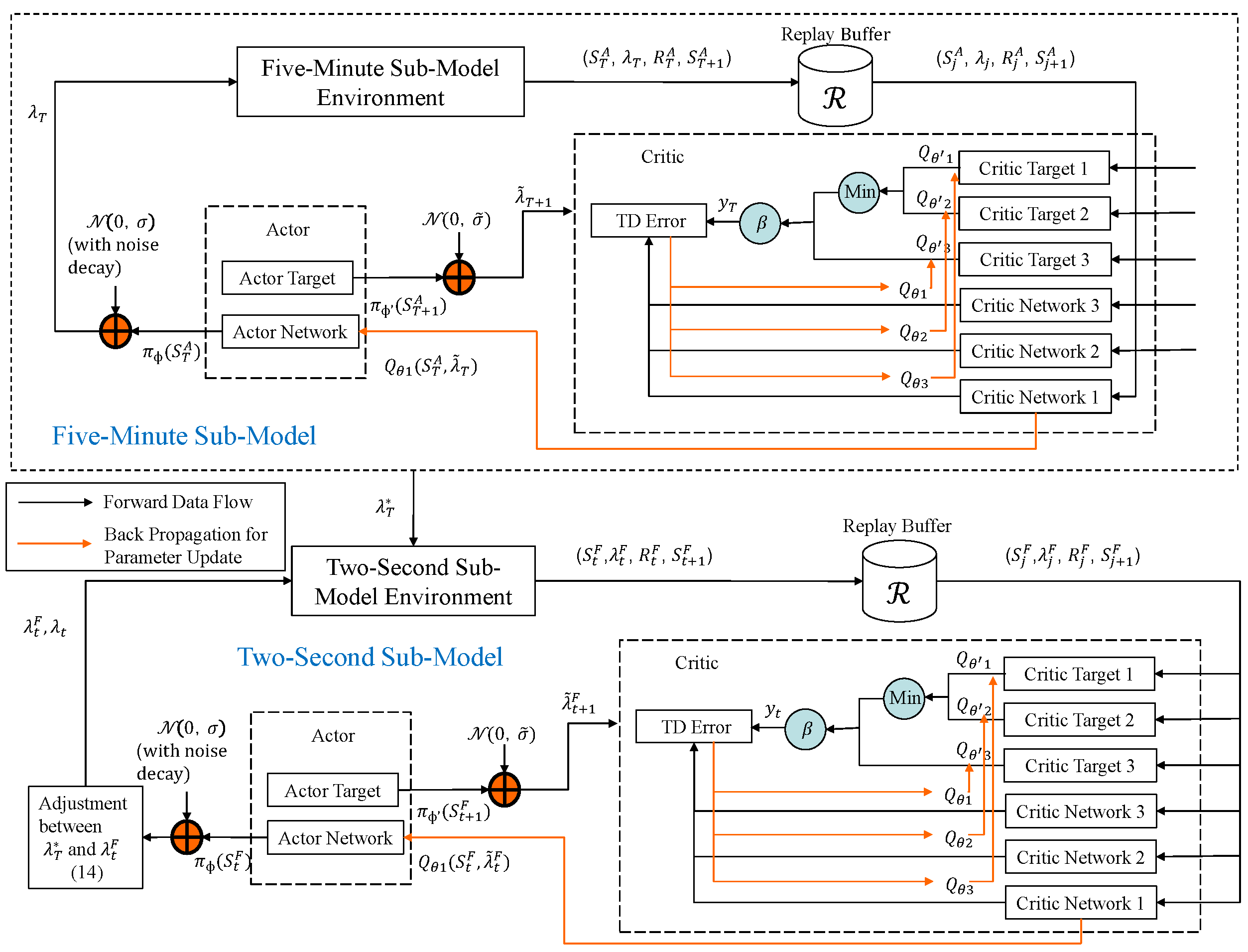
  • A novel co-optimization scheme is proposed to handle the multitimescale problem. The BESS decides an optimal EA action every five minutes to maximize its revenue due to the total amount of energy change, and every two seconds the BESS decides an optimal FR action to maximize the total reward including the revenue due to energy change and FR settlement reward. Based on the FR action, the EA action has to be adjusted based on the power constraints of the BESS to maximize the total revenue of the day on the two-second level.
  • The TDD–ND algorithm is proposed to solve the co-optimization problem. To the best of our knowledge, the TDD algorithm [34] is for the first time used for energy storage. Our proposed method combines the TDD algorithm with ND policy to improve the exploration during the training, and thus to achieve the higher total revenue.
  • Real-time data are used to evaluate the performance of the proposed TDD–ND co-optimization approach. Simulation results show that our proposed DRL approach with the co-optimization scheme performs better than studied policies.
The rest of this paper is organized as follows. Section 2 explains the Pennsylvania New Jersey Maryland (PJM)’s frequency regulation market. Section 3 presents the nested system model used to formulate the co-optimizing problem. Our proposed TDD–ND approach is described in Section 4. The simulation results are discussed in Section 5. The conclusion is made in Section 6.

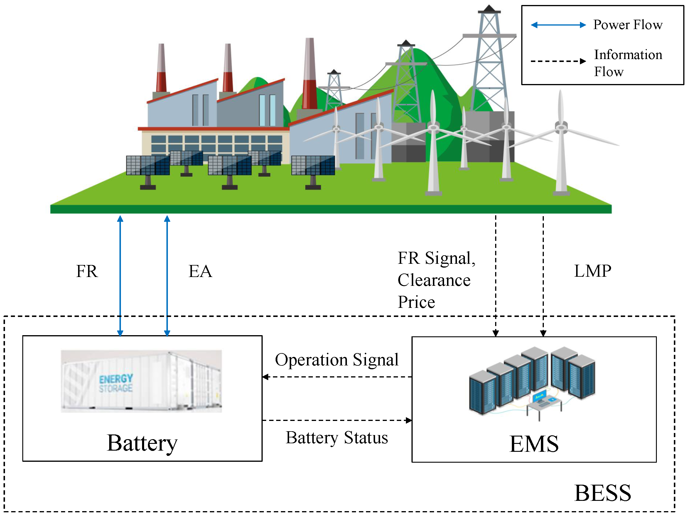
2. PJM Frequency Regulation Market

In the PJM frequency regulation market, generators and other devices (e.g., energy storage) can provide grid ancillary services in exchange for regulation credits [37]. PJM sends the regulation (RegD) signal to the resources wishing to provide regulation services every two seconds. Afterwards, PJM tracks the response from each resource and computes a performance score for each resource every two seconds based on the RegD signal and regulation response. For every five minutes, the market also calculates the average performance score within the five-minute period. The performance score is a weighted sum of correlation, delay, and precision [38,39]. A BESS typically has the nature of the instantaneous response and hence the scores of correlation and delay are close to 1. Therefore, the average performance score SC of a BESS within a five-minute period can be calculated based on the precision score as follows [19]:
S C = t = 0 150 Δ t S C t 150 ,
S C t = | 1 λ t F + r d t / a r | ,
where λ t F , r d t , a r are denoted as the regulation response power taken by BESS response to the RegD signal at time t, the RegD signal at time t, and the maximum power capacity assigned for FR, respectively. Δ t is set to two seconds because the RegD signal r d t is sent every two seconds. S C t denotes the two-second performance score. When the BESS is 100% following the RegD signal, λ t F + r d t = 0 and S C t = 1 .
Every five minutes, the PJM market determines the eligibility of the resource for regulation based on its average performance score S C , and calculates the amount of the regulation credit settlement received by the eligible resource. If the average performance score is less than 40%, the resource will lose its regulation qualification and regulation credits during that time period [37]. The five-minute regulation credit settlement R C can be calculated as follows [37]:
R C = S C · a r · P C , S C 0.4 , 0 , S C < 0.4 ,
where P C , in $ / MW · 5 min , is the five-minute regulation clearance price for 1 MW regulation capacity.

3. Nested System Model and Problem Formulation

The system model, illustrated in Figure 1, consists of two main parts, i.e., the power grid and the BESS including a battery and an energy management system (EMS). The BESS participates in the energy and regulation market. The power grid sends the real-time electricity locational marginal price (LMP), FR signal, and FR market clearance price to the EMS in the BESS. The EMS then generates the operation signal to the battery to take action. At the same time, the battery sends feedback with its real-time status to the EMS. Based on the real-time status of the battery and the information from the power grid, the EMS generates a new operation signal to the battery.
The BESS co-optimizes EA and FR services to maximize its total reward within a one-day time horizon in a real-time PJM market: EA acts every five minutes, and FR responds every two seconds [19]. Due to the nature of the problem, the timescale is divided into two dimensions: a large timescale with five-minute intervals and a small timescale with two-second intervals, where two-second intervals are nested in the five-minute timescales. The two optimization problems are formulated as two nested MDP submodels in the two following subsections, respectively.

3.1. The Five-Minute MDP Submodel Formulation

The one-day horizon of five-minute submodel T A , decomposed into 288 five-minute increments (i.e., Δ T = 5 min ) illustrated in Figure 2, is denoted as T A = { 0 , Δ T , 2 Δ T , 3 Δ T , 287 Δ T } . The BESS takes a charging or discharging action every five minutes based on its current state to maximize the cumulative reward within the one-day horizon. The state, action, and reward are defined as follows.

3.1.1. State

The state of the BESS at time T can be defined as S T A = E T , P T A , where E T is the BESS energy level, and P T A is the real-time electricity locational marginal price (LMP) at time T.

3.1.2. Action

The action in the five-minute submodel, denoted as λ T , is the total amount of power change due to EA and FR at time T within the five-minute interval. λ T > 0 represents that the BESS is charging, while λ T < 0 implies that the BESS is discharging. The optimal action at time T is denoted as λ T * . The action space should not exceed the maximum power capacity of BESS B:
λ T B .
The total amount of energy stored in the BESS at time T should be within its maximum energy capacity E max :
0 E T + λ T · Δ T E max .
After taking action λ T , state S T A is converted to state S T + Δ T A at time T + Δ T . The real-time price P T A is updated to P T + Δ T A , and the energy level E T evolves to E T + Δ T , which can be calculated as follows:
E T + Δ T = E T + Δ T · λ T · η c , λ T 0 , E T + Δ T · λ T / η d , λ T < 0 ,
where η c and η d denote the charging and discharging efficiency, respectively.

3.1.3. Degradation Cost and Reward

The degradation cost of the BESS is a key factor in energy operational planning [4] as the battery cells degrade for repeated charge/discharge cycles. The degradation cost of the BESS can be calculated as follows [4]:
f T ( b ) = c b λ T · Δ T ,
where c b is the degradation cost coefficient, and can be calculated as follows [4]:
c b = P c e l l 2 N · S O C max S O C min ,
where P c e l l is the price of the battery cell in the BESS and N is the number of cycles that the BESS could be operated within the state of charge (SoC) constraint [ S O C min , S O C max ].
After taking the action, the BESS will receive a reward. In order to avoid conservative actions caused by the negative reward in the learning process, an average electricity price P ¯ A is introduced in the reward R T A S T A , λ T for performing λ T action in state S T A based on the basic principle of EA [14] as follows:
R T A S T A , λ T = P ¯ A P T A · λ T · Δ T f T ( b ) .

3.2. The Two-Second MDP Submodel Formulation

The BESS needs to respond to the updated RegD signal every two seconds. Because two-second intervals are nested in the five-minute horizon, the time horizon of one day within every two-second increment is denoted as T F = { 0 , Δ t , 2 Δ t , 3 Δ t , ( 150 · 288 1 ) Δ t } , where Δ t = 2 s , shown in Figure 2. The BESS takes a charging or discharging action every two seconds based on its current state to maximize the cumulative reward within the one-day horizon. The state, action, and reward are defined as follows.

3.2.1. State

The state at time t is denoted as S t F = E t , r d t , where E t is the energy level of the BESS and r d t is the received RegD signal at that time.

3.2.2. Action

The action is the regulation response power, denoted as λ t F at time t, which is constrained by Equation (4). The action space also should not go beyond the maximum power capacity of BESS B. After performing an action λ t F at time t, state S t F will transfer to state S t + Δ t F at time t + Δ t , and the energy level E t will be updated to E t + Δ t based on λ t denoted as the total amount of power change at time t due to EA and FR:
E t + Δ t = E t + Δ t · λ t · η c , λ t 0 , E t + Δ t · λ t / η d , λ t < 0 .

3.2.3. Reward

Based on the PJM market regulation policy, the reward R t S t F , λ t F by performing action λ t F at state S t F can be calculated as
R t S t F , λ t F = R t A + R t F f t ( b ) ,
where f t ( b ) = c b λ t · Δ t according to Equation (7) and R t A is the reward due to the total amount of energy change caused by both EA and FR within the two-second interval:
R t A = P ¯ A P T A · λ t · Δ t .
Instead of calculating the FR settlement at the end of every five minutes, in the two-second submodel, we need to evaluate the FR reward every two seconds once choosing an action λ t . Based on Equation (3), R t F is the equivalent real-time regulation settlement reward within the two-second interval:
R t F = S C t · B · P C / 150 , S C t 0.4 , 0 , S C t < 0.4 ,
assuming that the maximum power capacity a r assigned for FR is the power capacity of the BESS B.

3.3. Proposed Co-Optimization Scheme

Solving the co-optimizing problem for EA and FR is to find the optimal action selection policy for the BESS to obtain the maximum expected reward within a day. A co-optimization scheme is proposed to handle the multitimescale problem and coordinate the EA and FR services, which is illustrated in Figure 3. Once λ t F is derived, λ t can be calculated as follows:
λ t = B + λ t F , λ T * λ t F > B , λ T * , λ T * λ t F B , B + λ t F , λ T * λ t F < B ,
where λ t is not always equal to λ T * , due to the power constraint (Equation (4)) of the BESS. The first case shows that when the optimal action for FR λ t F is discharging (i.e., λ t F < 0 ) and the best action for EA is charging, the action for EA will be charging with the highest power capacity B. In this case, the charging value of λ T * was set too high, and λ t is less than λ T * . For the second case, the λ t is set to λ T * . For the third case, when the optimal action for FR λ t F is charging and the best action for EA is discharging, the action for EA is discharging with the highest power capacity B . In this case, the discharging value of λ T * was set too low, and λ t is greater than λ T * .

4. Proposed Triplet Deep Deterministic Policy Gradient with Exploration Noise Decay Approach

A novel DRL approach, combining TDD [34] and ND, is proposed to address the co-optimization problem. TDD–ND is a model-free, off-policy actor–critic algorithm, in which the triplet critics are used to limit estimation bias, and the exploration ND policy is used to improve the exploration in the algorithm.

4.1. Triplet Deep Deterministic Policy Gradient Algorithm

The TDD algorithm [34] is an off-line RL algorithm which can be applied to solve the optimization problem with continuous state space as well as continuous actions [35,36]. TDD includes a single actor network (i.e., a deterministic policy network) π ϕ and its actor target network π ϕ . In addition, TDD adopts three critic networks Q θ 1 , Q θ 2 , and Q θ 3 for Q-value estimation. Q θ 1 , Q θ 2 and Q θ 3 represent three target networks, corresponding to critic networks Q θ 1 , Q θ 2 , and Q θ 3 , respectively. The target value y t can be updated using the weighted minimum Q-value of target Q-networks Q θ 1 and Q θ 2 , combined with the weighted value of Q θ 3 as follows [34]:
y t = r t + γ β min j { 1 , 2 } Q θ j s t + 1 , a ˜ t + 1 + ( 1 β ) Q θ 3 s t + 1 , a ˜ t + 1 ,
where β ( 0 , 1 ) is the weight of the pair of critics, γ [ 0 , 1 ] is a discount factor, and a ˜ t + 1 is the clipped target action, calculated as follows:
a ˜ t + 1 π ϕ s t + 1 + ϵ , ϵ clip ( N ( 0 , σ ˜ ) , c , c ) ,
where ϵ is the clipped Gaussian noise with standard deviation of σ ˜ , and c is the edge value. The parameters of the critic networks will be updated by minimizing the following loss:
L ( θ ) = E s t , a t , r t , s t + 1 R Q θ s t , a t y t 2 ,
where R is a replay buffer to store and relay experience transactions s t , a t , r t , s t + 1 including states, actions, rewards, and next states. The deterministic policy network in actor is updated using sampled policy gradient which is shown as follows:
ϕ J ( ϕ ) = N 1 a Q θ 1 ( s t , a t ) a = π ϕ ( s t ) ϕ π ϕ ( s t ) ,

4.2. Proposed TDD–ND Co-Optimization Approach

The ND policy is combined with the TDD algorithm to address the co-optimization problem. For the ND policy, the standard deviation of the exploration noise ϵ is set to the maximum value σ m a x at the beginning of the training, gradually reduced to the minimum value σ m i n with a decay of σ d e c a y with the increase of the number of the training episodes, and kept at the minimum value σ m i n for the rest of the training. A TDD–ND algorithm for five-minute submodel optimization is presented in Algorithm 1.
Algorithm 1: The TDD–ND training process for five-minute submodel optimization
Initialize the actor network π ϕ , the actor target network π ϕ π ϕ , the size R of replay buffer R , and the mini-batch size m.
Initialize the three critic networks Q θ 1 , Q θ 2 and Q θ 3 , and three critic target networks Q θ 1 Q θ 1 , Q θ 2 Q θ 2 and Q θ 3 Q θ 3 .
1:
 for episode i ← 0 to I do
2:
for   t T A do
3:
  Based on the state of the BESS S T A including E T and P T A , choose action λ T , observe reward R T A and next state of the BESS S T + 1 A .
4:
  Store transition S T A , λ T , R T A , S T + 1 A in R .
5:
  Sample a batch of transitions S j A , λ j , R j A , S j + 1 A from R .
6:
  From the next state of the BESS S T + 1 A , the actor target plays the next charging or discharging action of the BESS λ T + 1 via Equation (16).
7:
  Select Gaussian noise ϵ N ( 0 , σ ) to this next action λ T + 1 . Decrease σ from σ m a x to σ m i n with the decay of σ d e c a y as the increasing of the episode.
8:
  Calculate the estimated target value via Equation (15).
9:
  Update parameters of the three critic networks by minimizing the loss defined by Equation (17).
10:
  Update the weights of the critic target networks by: θ i τ θ i + ( 1 τ ) θ i , i = 1 , 2 , 3 every 2 iterations, where τ 1 is the target update parameter.
11:
  Update the actor network by performing gradient every 2 iterations based on Equation (18).
12:
  Update the weights of the actor target networks by: ϕ τ ϕ + ( 1 τ ) ϕ every 2 iterations.
13:
end for
14:
 end for
The flow chart of the proposed TDD–ND co-optimization approach is illustrated in Figure 3. The TDD–ND algorithm is used to train the neural networks for five-minute submodel optimization. The best actions of the five-minute submodel λ T * are then input into the two-second submodel environment. The TDD–ND algorithm is then used to train neural networks for two-second submodel optimization. For each training iteration, after action λ t F is chosen, λ t is calculated based on Equation (14), and the reward R T ( S t F , λ t F ) will be calculated using Equation (11) to maximize the accumulated reward within the one-day horizon. After each time step, a mini-batch of m transitions is sampled uniformly from a replay buffer   R .

5. Experimental Results

The performance of the proposed co-optimization approach is evaluated in a real-world scenario. The values of the parameters used in the simulations are listed in Table 1. Some of the parameters are varied in the simulation and will be noted accordingly. The parameter settings for the TDD–ND algorithm are listed in Table 2.

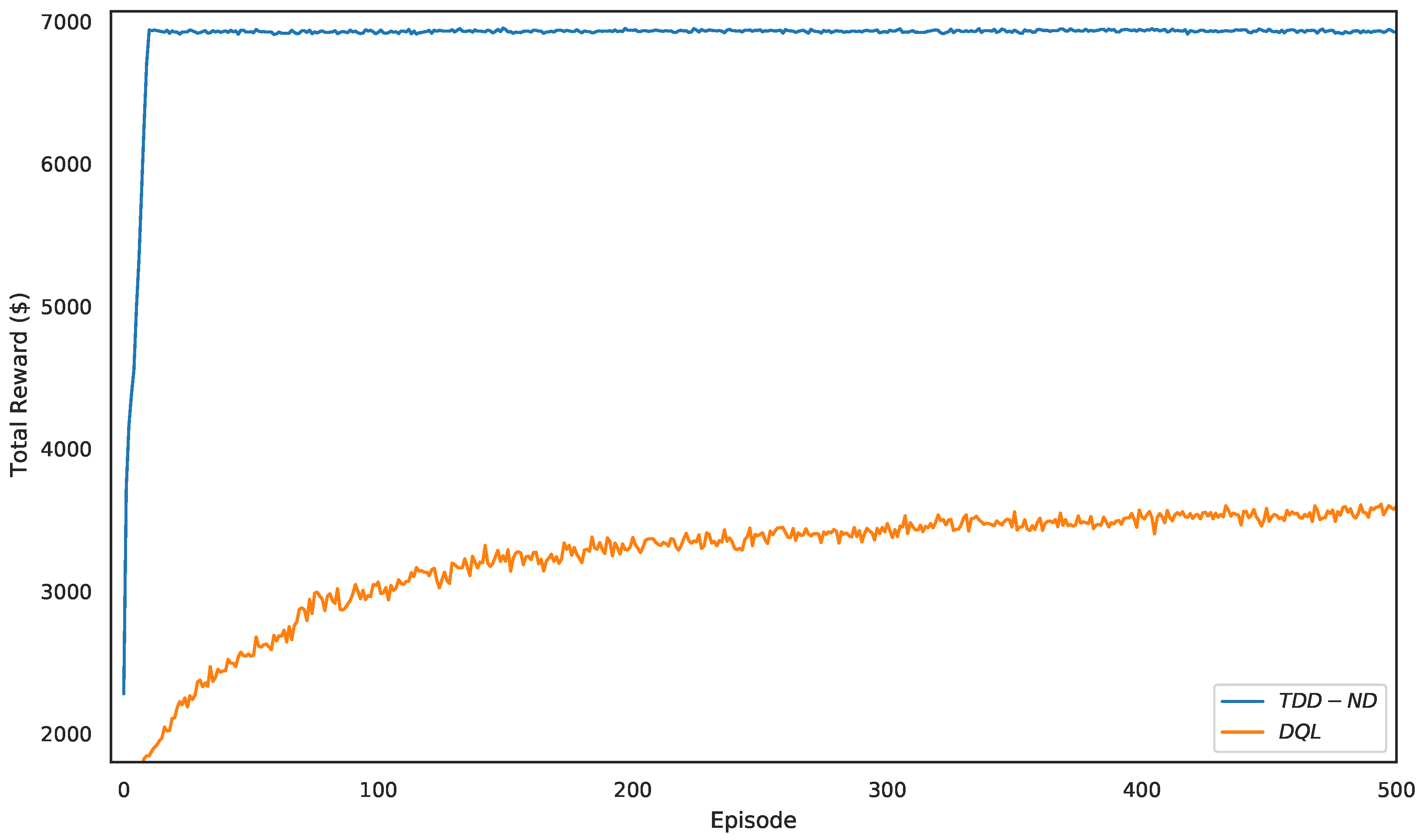
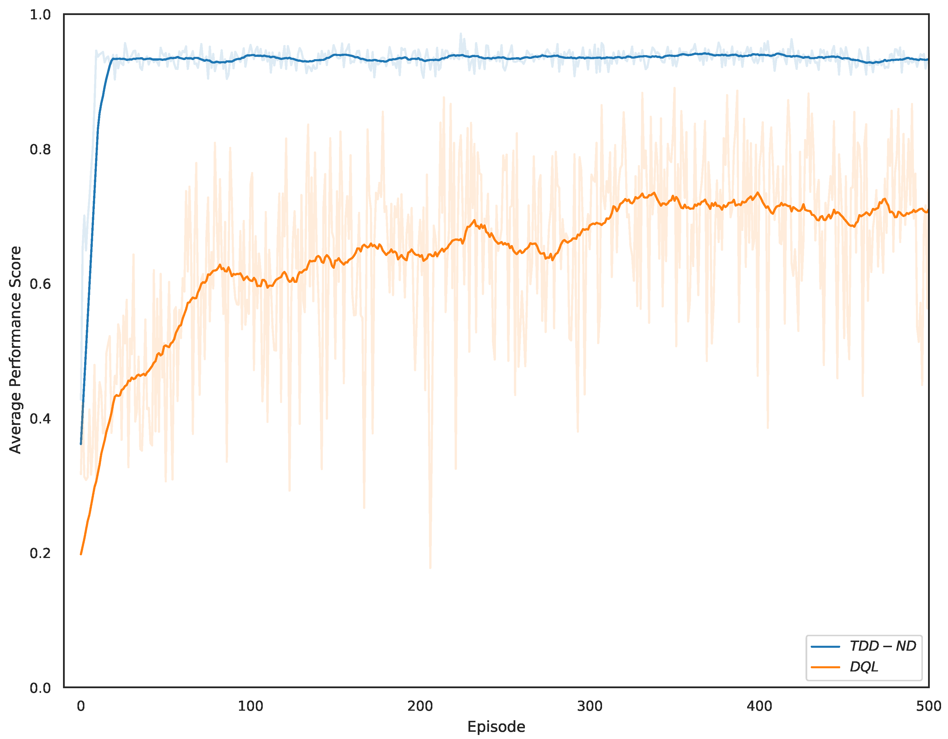
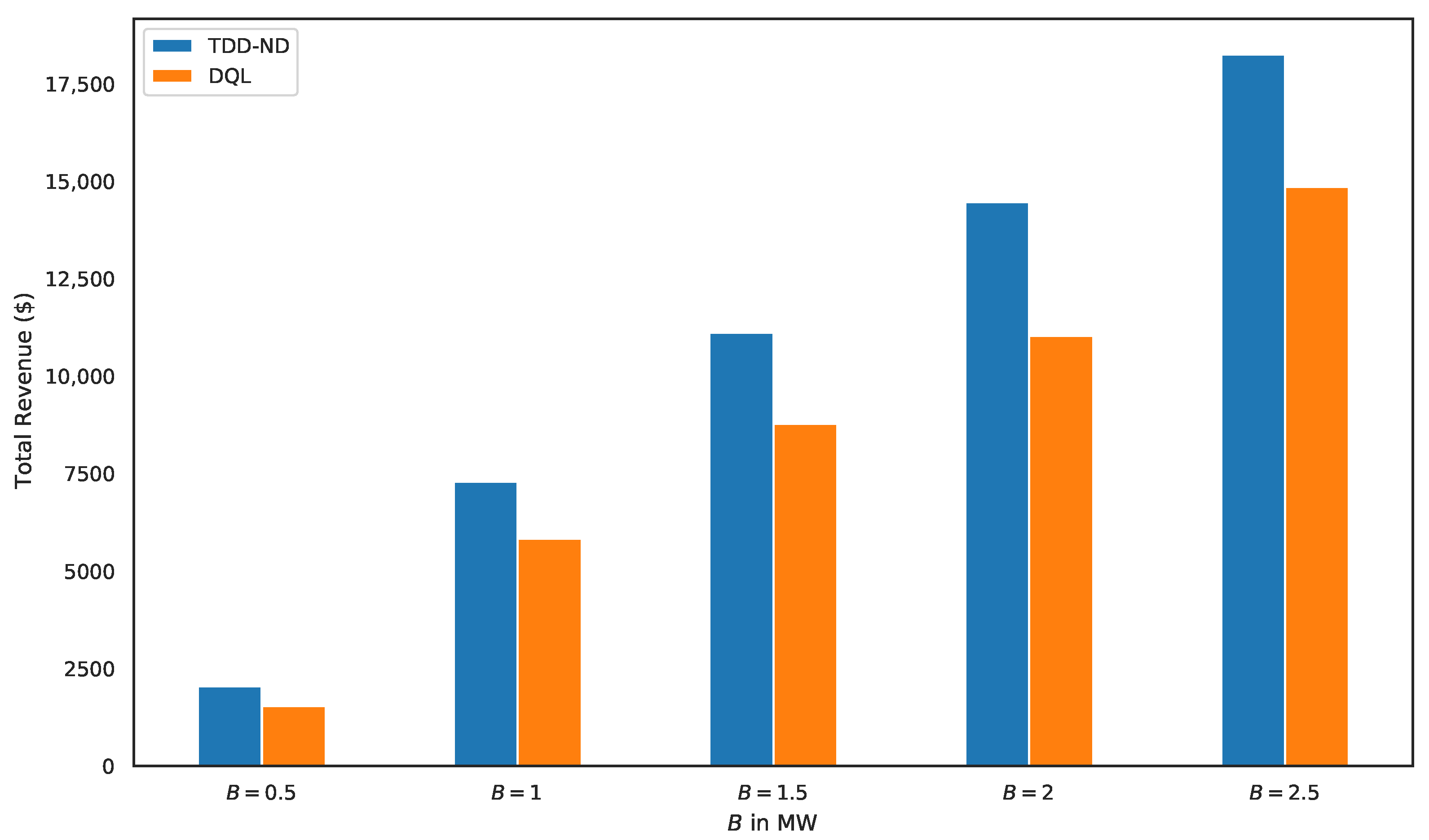
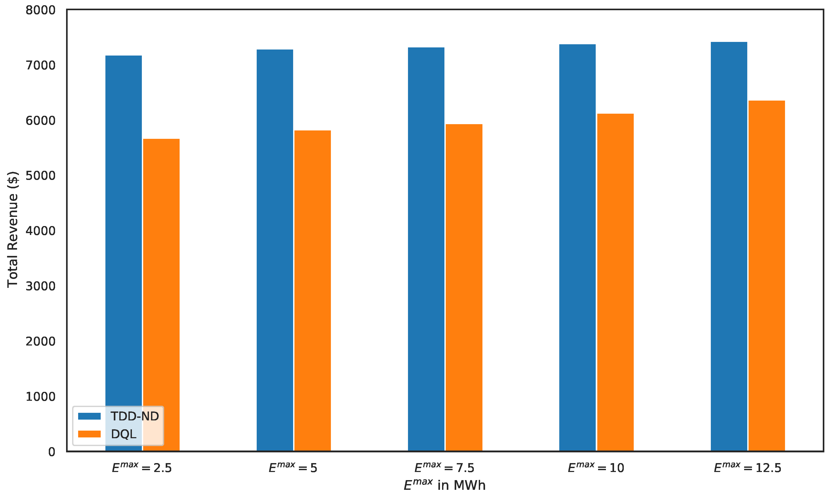
5.1. Performance Evaluation of the Proposed TDD–ND Algorithm

Based on the principle of EA, the BESS charges at low electricity prices and discharges at high electricity prices. The average price works as a simple indicator to determine whether the price P T A is low or high compared to the historical values. The operations of the BESS in a day are illustrated in Figure 4. The figure shows that when the P T A is lower than the average price, the BESS actions are mainly larger than 0, which means the BESS is charging. However, when the P T A is higher than the average price, the BESS operations are discharging to gain profits. The figure matches well with the principle of EA.
The performance of the TDD–ND algorithm for co-optimizing EA and FR is studied by comparing it with another widely-used DRL algorithm, the deep Q-learning (DQL) algorithm. TDD–ND and DQL algorithms were used to train the five-minute and two-second submodels for 500 times (500 episodes). During the training using TDD–ND, the total revenue of a day was validated after every 10 episodes without adding exploration noise ϵ to see whether the results were close to the training results. The learning curves of the TDD–ND algorithm and the DQL algorithm are illustrated in Figure 5 and Figure 6, respectively. These two figures show that the TDD–ND algorithm has a much better performance than the DQL algorithm in terms of the average performance score and the total reward. The reason is that the TDD–ND algorithm can choose more accurate continuous actions rather than using discretized actions in DQL, and can thus obtain a higher average performance score and total reward.
The impact of different levels of power capacity B and energy capacity E max on the performance of the TDD–ND algorithm and the DQL algorithm are studied. After training, the TDD–ND test results are slightly higher than their training values without the exploration noise. Figure 7 shows that the proposed TDD–ND algorithm always performs better than the DQL algorithm. The reason is that the DQL algorithm chooses discretized actions rather than continuous actions to take, and thus negatively impacts the total revenue. The figure also shows that the total revenue using both algorithms increases with power capacity B in the similar trend. For both algorithms, the total revenue increases sharply with B when B is between 0.5 and 1.0. The reason is that when B is 0.5, the S C t is smaller than 0.4 in most time slots, and thus the regulation settlement reward R t F becomes 0. When B increases to 1, the S C t is greater than 0.4 in many more time slots. Therefore, the total revenue is significantly increased. Between B = 1 and B = 2.5 , the improvement in total revenue approximately follows the increase of B, since R t F is the dominant factor in the total revenue, and is a linear function of B.
How energy capacity E max impacts the total revenue using the proposed TDD–ND algorithm and the DQL algorithm is shown in Figure 8. The figure shows that the TDD–ND algorithm generates more total revenue than the DQL algorithm under each of the E max settings. Compared to the impact of power capacity B, the increase of energy capacity E max only makes a slight change to the total revenue. For both algorithms, the total revenue rises slowly with the increase of E max between E max = 2.5 and 12.5, as the energy capacity increasing only improves R t A but R t F dominates the total revenue in Equation (11) when B = 1 MW. Compared to the TDD–ND algorithm, the DQL algorithm has a slightly higher improvement rate of the total reward with the increase of E max , since higher E max allows the DQL algorithm to choose better discretized actions for EA, and thus a higher improvement rate of R t A compared to the TDD–ND algorithm with continuous actions.

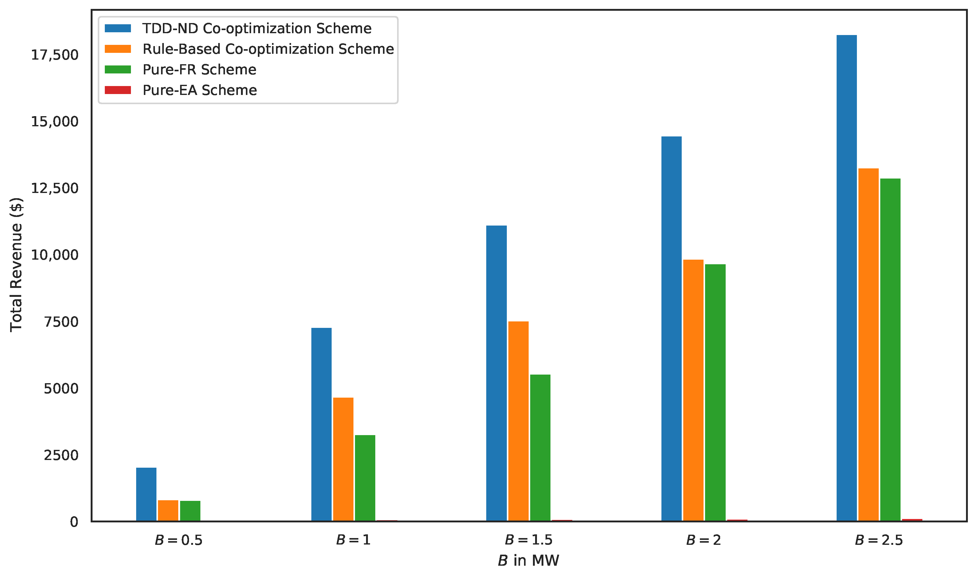
5.2. Performance Comparison of Various Schemes

To demonstrate the effectiveness of our proposed TDD–ND co-optimization scheme, the following methods are compared: (1) Pure-EA scheme, in which the BESS only provides the EA service; (2) Pure-FR scheme, in which the BESS only provides the FR service; (3) Rule-based co-optimization scheme, in which the BESS provides the EA and FR services. The rule is as follows: The action λ t is set to λ T * to maximize the reward due to the total amount of energy change caused by both EA and FR; (4) TDD–ND co-optimization scheme is our proposed TDD–ND algorithm and co-optimization scheme.
The total revenue using each scheme with different settings of B and E max is illustrated in Figure 9 and Figure 10, respectively. Figure 9 shows that the TDD–ND co-optimization scheme generates much more total revenue than the other three schemes at every setting of B, as the TDD–ND co-optimization scheme tries to maximize the total accumulated reward. The total revenue using the pure-EA scheme is very small, since FR is much more profitable than EA. For the TDD–ND scheme, the rule-based scheme and the pure-FR scheme, the regulation settlement reward R t F increases with B, and thus the total revenue increases with B. For the pure-EA scheme, the higher B allows the BESS to charge more when P T A is low and discharge more when P T A is high. The increasing rates of the total revenue using the TDD–ND co-optimization scheme and the rule-based co-optimization scheme from B = 0.5 to B = 1 are higher than those from B = 1 to B = 2.5. The reason is that when B = 0.5, the performance score is smaller than 0.4 in most time slots, and thus the regulation settlement reward becomes 0. Therefore, the total revenue of the rule-based co-optimization scheme is close to that of the pure-FR scheme. When B increases to 1, the performance score is greater than 0.4 in many more time slots, and with the coordination of EA, the total revenue is significantly increased. When B is between 1 and 1.5, the total revenue of the pure-FR scheme is much lower than that of the rule-based co-optimization scheme and that of the TDD–ND cop-optimization scheme. The reason is that the pure-FR scheme cannot follow r d t signals closely due to the limitations of the energy capacity, while the rule-based scheme can coordinate the energy capacity for EA and FR. When B reaches 2 or higher, the rule-based scheme has similar total revenue to the pure-FR scheme, as the setting of B allows the rule-based scheme to follow r d t signal closely.
The total revenue of each of the four schemes under different settings of energy capacities E max is presented in Figure 10. The total revenue of the proposed TDD–ND co-optimization scheme is much higher than those of the other three schemes. FR is much more profitable than EA under all of the E max settings. The total revenue of the TDD–ND scheme and the rule-based scheme increases slightly with E max , because the increase of E max only improves the value of R t A , which is a small portion of the total revenue R t . For the pure-EA scheme, the total revenue increases with energy capacity E max , as higher energy capacity allows the BESS to charge more when P T A is low and discharge more when P T A is high.

6. Conclusions

A battery energy storage system (BESS) providing both energy arbitrage (EA) and frequency regulation (FR) services simultaneously to maximize its total revenue within a day was considered. The BESS takes an EA action every five minutes and an FR action every two seconds. The multitimescale co-optimization problem was formulated as two nested Markov decision process (MDP) submodels. A novel co-optimization scheme was proposed to handle the multitimescale problem and to coordinate the EA and FR services to maximize the total revenue. The novel deep reinforcement learning (DRL) algorithm, triplet deep deterministic policy gradient with exploration noise decay (TDD–ND), was proposed to determine the best actions to take to maximize the accumulated reward within the one-day horizon. The proposed TDD–ND algorithm achieved 22.8% to 32.9% higher total revenue than the deep Q-learning (DQL) algorithm under various power capacity settings of the BESS when its energy capacity was 5 MWh, and achieved 16.7% to 26.6% higher total revenue under various energy capacity settings when the power capacity was 1 MW. Additionally, our proposed TDD–ND co-optimization scheme achieved 37.7% to 148.8%, 41.8% to 156.3%, and 3507.8% to 15,583.2% higher total revenues compared to the rule-based co-optimization scheme, the pure-FR scheme, and the pure-EA scheme, respectively, under various power capacity settings when the energy capacity of the BESS was 5 MWh. When the power capacity was set to 1 MW, the proposed TDD–ND co-optimization scheme achieved total revenues 49.6% to 56.2%, 51.0% to 198.4%, and 7156.2% to 12,777.0% higher than the rule-based co-optimization scheme, the pure-FR scheme, and the pure-EA scheme, respectively, under the various energy capacity settings. In the future, investigation can be carried out on the use of the co-optimization methods in multivector energy systems considering different timescales.

Author Contributions

Conceptualization, Y.M.; methodology, Y.M., T.C. and S.B.; software, Y.M., and T.C.; simulation, Y.M.; validation, Y.M.; formal analysis, Y.M.; investigation, Y.M., T.C. and S.B.; resources, Y.M. and S.B.; data curation, Y.M.; writing—original draft preparation, Y.M.; writing—review and editing, Y.M., S.B., H.L. and Z.H.; visualization, Y.M.; supervision, S.B.; project administration, Y.M., T.C. and S.B. All authors have read and agreed to the published version of the manuscript.

Funding

This work was supported by start-up funds provided by Brock University, NSF CNS-2128368, CNS-2107216, Toyota and Amazon.

Conflicts of Interest

The authors declare no conflict of interest.

Nomenclature

a r The maximum regulation capacity in MW assigned by PJM
BThe maximum power capacity of the BESS in MW
c b The linearized battery degradation cost co-efficient
E T Energy level of the BESS in MWh at time T in five-minute submodel
E t Energy level of the BESS in MWh at time t in two-second submodel
E m a x The maximum energy capacity of the BESS in MWh
f ( b ) The degradation cost
mThe mini-batch size
NThe number of cycles that the BESS
P T A The real-time electricity price at time T
P ¯ A The average value of electricity prices in the past day
P c e l l The price of the battery cell in the BESS
RegD Dynamic signal for fast regulation, which is a measure of the imbalance between
sources and uses of power in MW in the grid
r d t The regulation signal (RegD) sent by PJM at time t to the BESS to provide
regulation service
R C The five-minute regulation settlement
R T A The reward for performing an action λ T state S T A in five-minute submodel
R t The reward for performing action λ t F at state S t F in two-second submodel
R t F The real-time regulation settlement reward within the two-second interval
S C Average performance score within a five-minute period indicating the
performance of FR
S C t The two-second performance score at time t
S T A The state of five-minute submodel at time T
S t F The state of two-second submodel at time t
TThe time indicator in five-minute submodel
tThe time indicator in two-second submodel
T A The one-day horizon of five-minute submodel
T F The one-day horizon of two-second submodel
Δ T The five-minute time interval
Δ t The two-second time interval
λ T The action of the total amount of power change in MW due to EA and FR
at time T in five-minute submodel
λ t F The action in MW of BESS response to the RegD signal at time t in two-second
submodel
λ T * The optimal action of five-minute submodel at time T
λ t The total amount of power change at time t due to EA and FR in two-second
submodel
η c The charging efficiency of the BESS
η d The discharging efficiency of the BESS,
α a c t o r learning rate for actor
α c r i t i c learning rate for critic
σ m a x The maximum standard deviation value in the exploration noise
σ m i n The minimum standard deviation value in the exploration noise
σ d e c a y The decay of standard deviation value in the exploration noise decay policy
γ The discount factor for future rewards
R Replay buffer
RThe size of replay buffer
ϵ Clipped Gaussian noise
π ϕ The actor network in TDD–ND
π ϕ The actor target network in TDD–ND
Q θ Critic networks in TDD–ND
Q θ Target networks in TDD–ND

References

  1. Chatzinikolaou, E.; Rogers, D.J. A comparison of grid-connected battery energy storage system designs. IEEE Trans. Power Electron. 2017, 32, 6913–6923. [Google Scholar] [CrossRef]
  2. He, G.; Chen, Q.; Kang, C.; Pinson, P.; Xia, Q. Optimal bidding strategy of battery storage in power markets considering performance-based regulation and battery cycle life. IEEE Trans. Smart Grid 2016, 7, 2359–2367. [Google Scholar] [CrossRef] [Green Version]
  3. Rosewater, D.; Baldick, R.; Santoso, S. Risk-Averse Model Predictive Control Design for Battery Energy Storage Systems. IEEE Trans. Smart Grid 2020, 11, 2014–2022. [Google Scholar] [CrossRef]
  4. Shi, Y.; Xu, B.; Wang, D.; Zhang, B. Using battery storage for peak shaving and frequency regulation: Joint optimization for superlinear gains. IEEE Trans. Power Syst. 2018, 33, 2882–2894. [Google Scholar] [CrossRef] [Green Version]
  5. Meng, L.; Zafar, J.; Khadem, S.K.; Collinson, A.; Murchie, K.C.; Coffele, F.; Burt, G.M. Fast Frequency Response from Energy Storage Systems—A Review of Grid Standards, Projects and Technical Issues. IEEE Trans. Smart Grid 2020, 11, 1566–1581. [Google Scholar] [CrossRef] [Green Version]
  6. Arévalo, P.; Tostado-Véliz, M.; Jurado, F. A novel methodology for comprehensive planning of battery storage systems. J. Energy Storage 2021, 37, 102456. [Google Scholar] [CrossRef]
  7. Mohamed, N.; Aymen, F.; Ben Hamed, M.; Lassaad, S. Analysis of battery-EV state of charge for a dynamic wireless charging system. Energy Storage 2020, 2, 1–10. [Google Scholar] [CrossRef] [Green Version]
  8. Antoniadou-Plytaria, K.; Steen, D.; Tuan, L.A.; Carlson, O.; Fotouhi Ghazvini, M.A. Market-Based Energy Management Model of a Building Microgrid Considering Battery Degradation. IEEE Trans. Smart Grid 2021, 12, 1794–1804. [Google Scholar] [CrossRef]
  9. Avula, R.R.; Chin, J.X.; Oechtering, T.J.; Hug, G.; Mansson, D. Design Framework for Privacy-Aware Demand-Side Management with Realistic Energy Storage Model. IEEE Trans. Smart Grid 2021, 12, 3503–3513. [Google Scholar] [CrossRef]
  10. Arias, N.B.; Lopez, J.C.; Hashemi, S.; Franco, J.F.; Rider, M.J. Multi-Objective Sizing of Battery Energy Storage Systems for Stackable Grid Applications. IEEE Trans. Smart Grid 2020, 3053, 1–14. [Google Scholar] [CrossRef]
  11. Sioshansi, R.; Denholm, P.; Jenkin, T.; Weiss, J. Estimating the value of electricity storage in PJM: Arbitrage and some welfare effects. Energy Econ. 2009, 31, 269–277. [Google Scholar] [CrossRef]
  12. Cao, J.; Harrold, D.; Fan, Z.; Morstyn, T.; Healey, D.; Li, K. Deep Reinforcement Learning-Based Energy Storage Arbitrage with Accurate Lithium-Ion Battery Degradation Model. IEEE Trans. Smart Grid 2020, 11, 4513–4521. [Google Scholar] [CrossRef]
  13. Eyer, J.M.; Iannucci, J.J.; Corey, G.P.; SANDIA. Energy storage benefits and markets analysis handbook. In A Study for DOE Energy Storage Systems Program; Sandia National Laboratories: Albuquerque, NM, USA; Livermore, CA, USA, 2004; p. 105. [Google Scholar]
  14. Wang, H.; Zhang, B. Energy storage arbitrage in real-time markets via reinforcement learning. In Proceedings of the IEEE Power and Energy Society General Meeting, Portland, OR, USA, 5–9 August 2018; pp. 1–5. [Google Scholar]
  15. Abdulla, K.; De Hoog, J.; Muenzel, V.; Suits, F.; Steer, K.; Wirth, A.; Halgamuge, S. Optimal operation of energy storage systems considering forecasts and battery degradation. IEEE Trans. Smart Grid 2018, 9, 2086–2096. [Google Scholar] [CrossRef]
  16. Chen, Y.; Hashmi, M.U.; Deka, D.; Chertkov, M. Stochastic Battery Operations using Deep Neural Networks. In Proceedings of the 2019 IEEE Power and Energy Society Innovative Smart Grid Technologies Conference, ISGT 2019, Washington, DC, USA, 18–21 February 2019; pp. 7–11. [Google Scholar]
  17. Krishnamurthy, D.; Uckun, C.; Zhou, Z.; Thimmapuram, P.R.; Botterud, A. Energy storage arbitrage under day-ahead and real-time price uncertainty. IEEE Trans. Power Syst. 2017, 33, 84–93. [Google Scholar] [CrossRef]
  18. Grid Energy Storage; Tech. Rep.; Dept. Energy: Washington, DC, USA, 2013.
  19. Cheng, B.; Powell, W.B. Co-optimizing battery storage for the frequency regulation and energy arbitrage using multi-scale dynamic programming. IEEE Trans. Smart Grid 2018, 9, 1997–2005. [Google Scholar] [CrossRef]
  20. Cheng, B.; Asamov, T.; Powell, W.B. Low-rank value function approximation for co-optimization of battery storage. IEEE Trans. Smart Grid 2018, 9, 6590–6598. [Google Scholar] [CrossRef]
  21. Walawalkar, R.; Apt, J.; Mancini, R. Economics of electric energy storage for energy arbitrage and regulation in New York. Energy Policy 2007, 35, 2558–2568. [Google Scholar] [CrossRef]
  22. Perekhodtsev, D. Two Essays on Problems of Deregulated Electricity Markets. Ph.D. Thesis, Carnegie Mellon University, Pittsburgh, PA, USA, 2004; p. 94. [Google Scholar]
  23. Engels, J.; Claessens, B.; Deconinck, G. Optimal Combination of Frequency Control and Peak Shaving with Battery Storage Systems. IEEE Trans. Smart Grid 2019, 11, 3270–3279. [Google Scholar] [CrossRef] [Green Version]
  24. Sun, Y.; Bahrami, S.; Wong, V.W.; Lampe, L. Chance-constrained frequency regulation with energy storage systems in distribution networks. IEEE Trans. Smart Grid 2020, 11, 215–228. [Google Scholar] [CrossRef]
  25. Jiang, T.; Ju, P.; Wang, C.; Li, H.; Liu, J. Coordinated Control of Air-Conditioning Loads for System Frequency Regulation. IEEE Trans. Smart Grid 2021, 12, 548–560. [Google Scholar] [CrossRef]
  26. Tian, Y.; Bera, A.; Benidris, M.; Mitra, J. Stacked Revenue and Technical Benefits of a Grid-Connected Energy Storage System. IEEE Trans. Ind. Appl. 2018, 54, 3034–3043. [Google Scholar] [CrossRef]
  27. Nguyen, T.T.; Nguyen, N.D.; Nahavandi, S. Deep reinforcement learning for multi-agent systems: A review of challenges, solutions and applications. IEEE Trans. Cybern. 2018, 50, 3826–3839. [Google Scholar] [CrossRef] [PubMed] [Green Version]
  28. Chen, T.; Bu, S.; Liu, X.; Kang, J.; Yu, F.R.; Han, Z. Peer-to-Peer Energy Trading and Energy Conversion in Interconnected Multi-Energy Microgrids Using Multi-Agent Deep Reinforcement Learning. IEEE Trans. Smart Grid 2021. [Google Scholar] [CrossRef]
  29. Wang, B.; Li, Y.; Ming, W.; Wang, S. Deep Reinforcement Learning Method for Demand Response Management of Interruptible Load. IEEE Trans. Smart Grid 2020, 11, 3146–3155. [Google Scholar] [CrossRef]
  30. Wu, J.; Wei, Z.; Li, W.; Wang, Y.; Li, Y.; Sauer, D.U. Battery Thermal-and Health-Constrained Energy Management for Hybrid Electric Bus Based on Soft Actor-Critic DRL Algorithm. IEEE Trans. Ind. Inform. 2021, 17, 3751–3761. [Google Scholar] [CrossRef]
  31. Wu, J.; Wei, Z.; Liu, K.; Quan, Z.; Li, Y. Battery-Involved Energy Management for Hybrid Electric Bus Based on Expert-Assistance Deep Deterministic Policy Gradient Algorithm. IEEE Trans. Veh. Technol. 2020, 69, 12786–12796. [Google Scholar] [CrossRef]
  32. Wei, Z.; Quan, Z.; Wu, J.; Li, Y.; Pou, J.; Zhong, H. Deep Deterministic Policy Gradient-DRL Enabled Multiphysics-Constrained Fast Charging of Lithium-Ion Battery. IEEE Trans. Ind. Electron. 2021. [Google Scholar] [CrossRef]
  33. Fujimoto, S.; Van Hoof, H.; Meger, D. Addressing Function Approximation Error in Actor-Critic Methods. In Proceedings of the 35th International Conference on Machine Learning, ICML 2018, Stockholm, Sweden, 10–15 July 2018; Volume 4, pp. 2587–2601. [Google Scholar]
  34. Wu, D.; Dong, X.; Shen, J.; Hoi, S.C. Reducing Estimation Bias via Triplet-Average Deep Deterministic Policy Gradient. IEEE Trans. Neural Netw. Learn. Syst. 2020, 31, 4933–4945. [Google Scholar] [CrossRef]
  35. Lillicrap, T.P.; Hunt, J.J.; Pritzel, A.; Heess, N.; Erez, T.; Tassa, Y.; Silver, D.; Wierstra, D. Continuous control with deep reinforcement learning. In Proceedings of the 4th International Conference on Learning Representations, ICLR 2016—Conference Track Proceedings, San Juan, PR, USA, 2–4 May 2016. [Google Scholar]
  36. Shi, Q.; Lam, H.K.; Xuan, C.; Chen, M. Adaptive neuro-fuzzy PID controller based on twin delayed deep deterministic policy gradient algorithm. Neurocomputing 2020, 402, 183–194. [Google Scholar] [CrossRef]
  37. PJM. PJM Manual 11: Services, Ancillary Operations, Market Operations, Real-Time Market; PJM: Valley Forge, PA, USA, 2019. [Google Scholar]
  38. Croop, D. PJM—Performance Scoring, Regulation Market Issues Senior Task Force; PJM: Valley Forge, PA, USA, 2016. [Google Scholar]
  39. Operations, B.; Pilong, C. PJM Manual 12: Regulation; PJM: Valley Forge, PA, USA, 2016. [Google Scholar]
  40. PJM. Real-Time Five Minute LMPs; PJM: Valley Forge, PA, USA, 2019. [Google Scholar]
  41. PJM. Ancillary Services; PJM: Valley Forge, PA, USA, 2019. [Google Scholar]
Figure 1. The configuration of the system model.
Energies 14 08365 g001
Figure 2. The nested timescales in a day.
Energies 14 08365 g002
Figure 3. The TDD–ND approach for the proposed co-optimization scheme.
Energies 14 08365 g003
Figure 4. The BESS operation in a one-day period after five-minute submodel optimization.
Energies 14 08365 g004
Figure 5. The learning curve of the average performance score of the day trained by TDD–ND and DQL.
Energies 14 08365 g005
Figure 6. The learning curves of TDD–ND and DQL of the total revenue within a day.
Energies 14 08365 g006
Figure 7. The total revenue of the day with different levels of power capacity B.
Energies 14 08365 g007
Figure 8. The total revenue of the day with different levels of energy capacity E max .
Energies 14 08365 g008
Figure 9. The comparison of the total revenues between using our proposed TDD–ND co-optimization scheme, rule-based co-optimization scheme, pure-FR scheme, and pure-EA scheme under different levels of power capacity B.
Energies 14 08365 g009
Figure 10. The comparison of the revenues between following the proposed TDD–ND co-optimization, rule-based co-optimization, and pure-FR and pure-EA schemes under different settings of energy capacity E max .
Energies 14 08365 g010
Table 1. The value of the parameters used in the simulation.
ParametersValue
P T A PJM historical real-time LMP from 00:00:00 AM
to 11:55:00 PM, 30 July 2021 [40]
P C PJM historical real-time clearance price for FR from 00:00:00 AM to
11:55:00 PM, 30 July 2021 [40]
r d t Historical real-time RegD signal from 00:00:00 AM to
11:59:58 PM, 30 July 2021 [41]
E max 5 MWh
B, a r 1 MW
P c e l l 8 × 10 4 $ / MWh
C b 4/MWh
Table 2. TDD–ND parameter settings.
ParametersValue
α a c t o r 8 × 10 4
α c r i t i c 8 × 10 5
γ 0.99
σ m a x 1
σ m i n 0.01
σ d e c a y 3 × 10 3
R 1 × 10 6
m 1 × 100
Publisher’s Note: MDPI stays neutral with regard to jurisdictional claims in published maps and institutional affiliations.

