Nonlinear Moving Boundary Model of Low-Permeability Reservoir

Abstract

At present, there are two main methods for solving oil and gas seepage equations: analytical and numerical methods. In most cases, it is difficult to find the analytical solution, and the numerical solution process is complex with limited accuracy. Based on the mass conservation equation and the steady-state sequential substitution method, the moving boundary nonlinear equations of radial flow under different outer boundary conditions are derived. The quasi-Newton method is used to solve the nonlinear equations. The solutions of the nonlinear equations with an infinite outer boundary, constant pressure outer boundary and closed outer boundary are compared with the analytical solutions. The calculation results show that it is reliable to solve the oil-gas seepage equation with the moving boundary nonlinear equation. To deal with the difficulty in solving analytical solutions for low-permeability reservoirs and numerical solutions of moving boundaries, a quasi-linear model and a nonlinear moving boundary model were proposed based on the characteristics of low-permeability reservoirs. The production decline curve chart of the quasi-linear model and the recovery factor calculation chart were drawn, and the sweep radius calculation formula was also established. The research results can provide a theoretical reference for the policy-making of development technology in low-permeability reservoirs.

1. Introduction

Classical Darcy’s law [1] has been widely used to describe seepage mechanics and numerical simulation for a long time. However, in recent years, the experimental monitoring data of pore seepage in tight oil and gas reservoirs, such as shale oil and gas, low-permeability oil and gas reservoirs and weak permeable layers, confirm that the fluid seepage in low-permeability tight media does not follow Darcy’s law, and the seepage velocity and pressure gradient reflected from the seepage characteristic curve is not linear. The study of nonlinear seepage in tight media has important guiding significance and application value for the effective development of tight oil and gas reservoirs.

Bear [2] proposed the concept of starting pressure gradient and gave the non-Darcy seepage equation of low-permeability formation during the process of studying the seepage mechanism of low-permeability formation through a laboratory test with a one-dimensional core in 1972. Prada [3] and Civan [3,4] found that the linear fitting curve of seepage velocity and pressure gradient experimental data had obviously deviated from the origin in the experimental study of rock fluid flow in different low-permeability porous media, and they developed the quasi-linear motion equation by modifying the Darcy equation.

$$q=A\frac{k}{\mu }(J-J_0)$$

(1)

When J ≤ J₀, q = 0; and J > J₀, fluid flow occurs in the porous media.

Ding [5] carried out new experiments to determine threshold pressure gradient (TPG) by designing a specially core-flooding system under reservoir conditions; the experimental result indicates that TPG is not constant during the reservoir developing process and varies with the change of pore pressure.

Huang Yanzhang [6] studied the causes of the fluid flow and pressure gradient deviating from Darcy’s law in dense media through a seepage experiment at a rather early stage. The causes of the non-Darcy seepage phenomenon can be summarized as follows: On the one hand, the dense porous media has narrow pores and a large surface area, the interface between rock and fluid is strong, and the micro-scale effect is severe; surface active substances will adsorb on the inner surface of the rock to form a boundary layer, which hinders fluid flow. On the other hand, due to the different throat radius of dense porous media, strong rock heterogeneity, and the small driving pressure gradient, the fluid can only flow along the central part of the large throat. With the increase in the driving pressure gradient, the thickness of the boundary layer gradually becomes thinner, and more fluid can participate in the flow at the middle and edge of small and large channels, so that the effective permeability of the rock gradually increases to the maximum, that is, the absolute permeability of the rock. As a result, the fluid seepage law in dense porous media does not follow the traditional linear Darcy’s law and will present strong nonlinear flow characteristics.

Dou H E [7] stated that the experiment conditions, the experiment process and the core sample preparation process are the three main reasons for the obvious TPG measured from the low permeability core experiments.

This is necessary to determine the starting pressure gradient when the quasi-linear seepage model is used. Huang Yanzhang used the capillary flow formula to obtain the theoretical calculation formula of the starting pressure gradient.

$$\lambda ={\tau }_{\mathrm{o}}\sqrt{\frac{8\varphi }{9K}}$$

(2)

where λ is the start-up pressure gradient, MPa/cm; τ_o is the ultimate shear stress, N; K is the core air permeability, 10⁻³μm²; ϕ is the porosity.

For the convenience of calculation, many experts and scholars have conducted laboratory experiments to obtain an empirical formula for calculating the starting pressure gradient. Chengyuan Lu [8] selected sandstone reservoir cores from 10 oilfields in the Shengli Oilfield in 2002 to represent low-permeability sandstone reservoirs in the Shengli Oilfield. The start-up pressure gradient of single-phase oil phase percolation and the air permeability of the sample were measured by the capillary balance method, and the empirical formula for the start-up pressure gradient was established by the linear regression method, which would be a better way to meet the requirements of engineering calculations.

The commercial reservoir numerical simulator represented by Eclipse is developed based on the linear Darcy flow law, which cannot accurately describe the nonlinear flow characteristics existing in the developing process of low-permeability reservoirs. Even with the simplest quasi-linear non-Darcy flow model, the common reservoir numerical simulators can produce significant errors in the optimization design of reservoir development parameters, such as well pattern and spacing and recovery factors. For low-permeability reservoirs, when the oil and water seepage occurs in the formation during production, the area where the formation pressure gradient is greater than the start-up pressure gradient is the pressure drop sweep area; the area where the formation pressure gradient is less than the starting pressure gradient is the non-sweep area; and the formation pressure in this area remains as the original formation pressure. On the boundary between the two regions, the formation pressure gradient is equal to the starting pressure gradient. As the seepage process in the reservoir is unstable, the pressure gradient in the low-permeability formation also changes, resulting in the boundary between the two regions moving with time and space. The mathematical expression that characterizes the moving boundary in mathematical modeling is called the moving boundary condition. The model based on the quasi-linear seepage equation is actually a moving boundary problem. In 1981, H. Pascal [9] first studied the one-dimensional unsteady seepage flow boundary model in porous media with a start-up pressure gradient, solved the model by an approximate analytical method and numerical method, and then analyzed the influence of the start-up pressure gradient on pressure and flow distribution in the flow system. In 1992, WuY.S. [10,11] used the law of flow continuity and conservation of mass to obtain the approximate analytical solution of the control partial differential equation in the sense of an average integral using the integration method and established the corresponding reservoir test interpretation method. In 2008, Feng [12] studied the unstable radial seepage model in a low-permeability gas reservoir considering the start-up pressure gradient through the numerical approximate Green function method; the results show that the moving boundary can characterize the control radius of a single well. Chen [13] used pore scale network modeling to study the seepage and displacement of porous media with the starting pressure gradient or yield stress. Lu J. [14,15] presented a boundary-dominated flow model in radial shape geometry and developed the analytical solutions. Yun [16,17] proposed a fractal model of starting pressure gradient in the flow process of non-Newtonian Bingham fluid in porous media. In 2010, Xie K. H [18] obtained a general approximate analytical solution for a one-dimensional clay soil consolidation moving boundary model considering the starting pressure gradient. Liu et al. [19] discussed analytical and numerical solutions of a semi-infinite low permeability reservoir under one-dimensional flow with a moving boundary and TPG. However, their solutions, which are processed by similarity transformations, are complicated and difficult, and the influence of the TPGs is not obvious. Wang Xiao-dong [20] proposed the analytical solutions under fixed-borehole-rate and fixed-borehole-pressure by applying Green’s function. Two transcendental equations for the moving boundary model were obtained and solved by using the Newton–Raphson iteration. Huang Y [21] presented a new unsteady production decline model of dual-porosity medium (matrix and fracture) and composite gas reservoir, proposed a complex mathematical solution, and discussed the influence of different reservoir parameters on the production decline regularity of composite reservoirs.

The approximate analytical solution, numerical solution, Bundle of capillary tube modeling (BCTM), direct pore scale modeling (DPSM) and Pore Network Modeling (PNM) are the main research methods and tools; however, the exact analytical solution of a porous media seepage flow boundary model with the starting pressure gradient, the proof of the existence of the solution and the moving law of the moving boundary are rarely studied. Various nonlinear seepage models based on laboratory experiments and theoretical derivation enrich the seepage theory of low-permeability reservoirs, but most models greatly increase the difficulty of calculation and are difficult to use in engineering. From the perspective of engineering calculation and calculation error, the quasi-linear model can better simulate the seepage mechanism of low-permeability reservoirs, and it is the mainstream of seepage theory research on a low-permeability reservoir.

When the steady-state sequential replacement method is used to solve the unstable seepage problems, it often regards each instantaneous state of the unstable seepage process as stable, and this can transform the unstable seepage partial differential equation into an ordinary differential equation without time. Numerous researchers are inclined to apply it to solve the flow radius of different reservoir models.

The quasi-linear seepage model of a low-permeability reservoir is used within the moving boundary, and the fluid flow does not occur outside the moving boundary. Based on this idea, this paper deduces and establishes the nonlinear moving boundary equation based on the steady-state sequential replacement method, which can be accurately and simply used to solve the quasi-linear model of a low-permeability reservoir. By solving the model, the calculation chart of recovery factor, sweep radius and other parameters of low permeability reservoirs under different starting pressure gradients can be obtained. In our model, only a nonlinear formula needs to be solved at each time-step, which achieves the same result with low-permeability reservoir numerical simulation. Therefore, smaller errors according to the analytic solution and fewer calculations compared to a routine numerical simulation method are the two maximum advantages of our model. This research provides a new idea for nonhomogeneous partial differential equations as well. The results can provide a theoretical reference for low-permeability reservoir development technology policy formulation and numerical simulation of low-permeability reservoirs.

2. Moving Boundary Nonlinear Equation

2.1. Darcy Flow of Conventional Reservoir

2.1.1. Mathematical Model

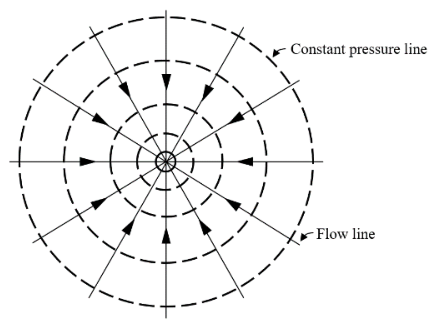
To facilitate the derivation, take the simplest plane radial flow model as an example (Figure 1).

Basic assumptions are as follows:

①

The reservoir is isotropic homogeneous and has a circular shape with equal thickness, closed top and bottom, and uniform original formation pressure;

②

The fluid is single-phase and micro-compressible, seepage flow is under constant temperature without physical and chemical changes and satisfies Darcy’s law;

③

Permeability, porosity, compressibility, and viscosity, etc., are all constants and do not change with time or pressure;

④

The influence of gravity is not considered, and the pressure gradient is small.

Considering a constant pressure production well in the center of a circular homogeneous area, the seepage equation is as follows:

$$\frac{1}{r}\frac{\partial }{\partial r}(r\frac{\partial p}{\partial r})=\frac{\mu \varphi C_t}{k}\frac{\partial p}{\partial t}$$

(3)

Constant pressure inner boundary conditions:

$$p{\left|\right.}_{r_w}=p_w$$

(4)

Infinite boundary:

$$\underset{r\to \infty }{\lim }p=p_i$$

(5)

Stable boundary:

$$p{\left|\right.}_{r_e}=p_i$$

(6)

Closed boundary:

$$p\prime {\left|\right.}_{r_e}=0$$

(7)

2.1.2. Moving Boundary Nonlinear Equation

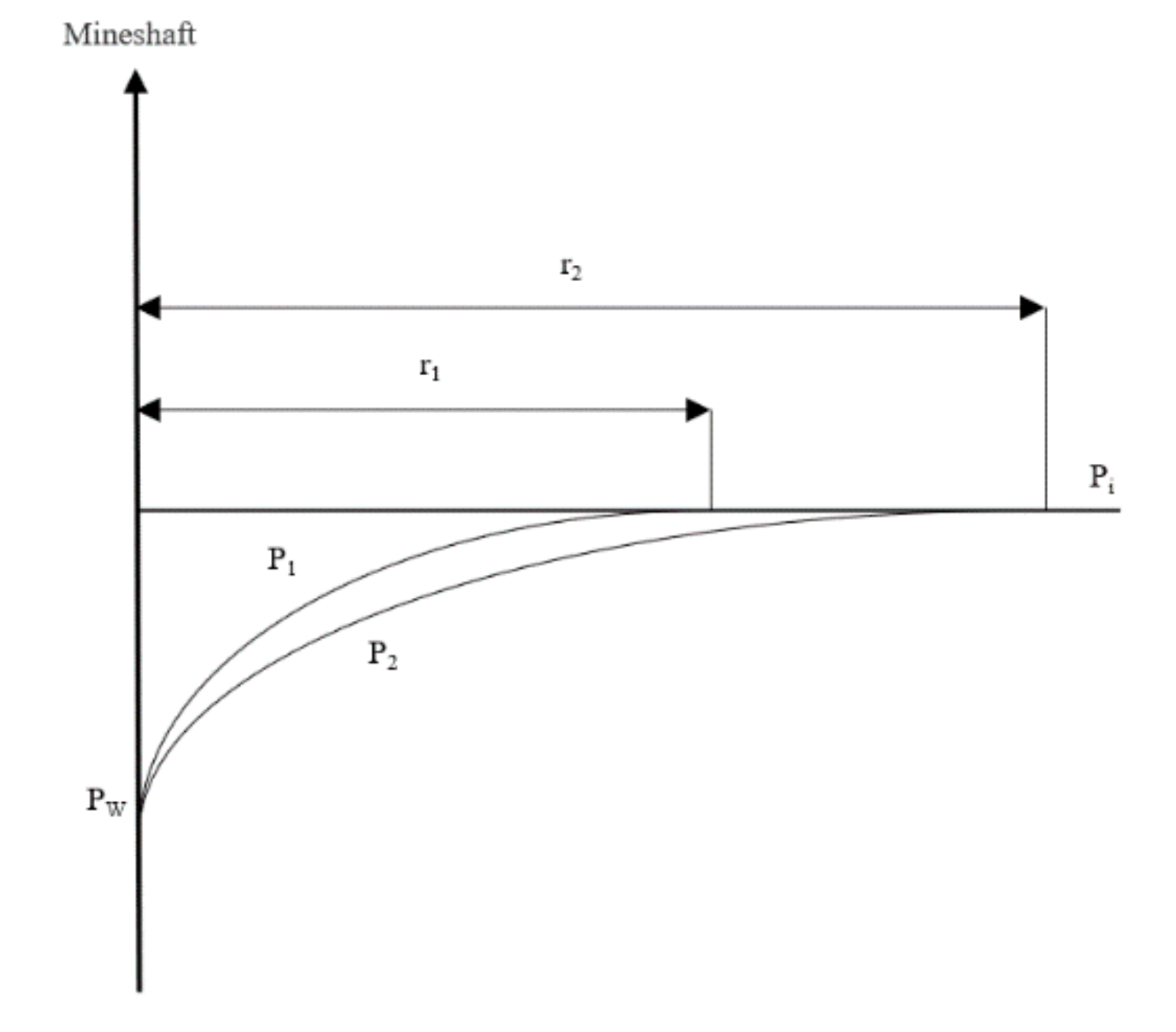
Steady state sequential replacement method [22]: when solving a series of problems related to the unstable seepage, each instantaneous state of the unstable seepage process is often regarded as stable. Considering the time period t₁→t₁ + Δt, the pressure sweep radius is from r₁→r₂ (see Figure 2).

Steady state pressure equation:

$$\frac{1}{r}\frac{\partial }{\partial r}(r\frac{\partial p}{\partial r})=0$$

(8)

The formation pressure P₁ distribution at time t is obtained by an integral solution:

$$p_1=\frac{p_i-p_w}{\ln \frac{r_1}{r_w}}\ln r+\frac{p_w\ln r_1-p_i\ln r_w}{\ln \frac{r_1}{r_w}}$$

(9)

The formation pressure P₂ distribution at time t + Δt can be obtained similarly.

$$p_2=\frac{p_i-p_w}{\ln \frac{r_2}{r_w}}\ln r+\frac{p_w\ln r_2-p_i\ln r_w}{\ln \frac{r_2}{r_w}}$$

(10)

Dimensionless bottom-hole production calculation formula:

$$q_D=\frac{\mu q}{2\pi kh(p_i-p_w)}=\frac{1}{\ln r_{iD}}$$

(11)

Among them:

t_D is dimensionless time, dimensionless, $t_{\mathrm{D}}=\frac{3.6kt}{\varphi \mu C{r}_{\mathrm{w}}^2}$;

r_i is dimensionless radius, dimensionless, $r_{iD}=\frac{r_i}{r_w},i=1,2$;

p_D is dimensionless pressure, dimensionless, $p_D=\frac{p_i-p}{p_i-p_w}$ ;

q_D is dimensionless flowrate, dimensionless, $q_D=\frac{\mu q}{2\pi kh\left(p_i-p_w\right)}$;

The same is shown below.

With the increase in r_iD, the yield decreased gradually.

Mass conservation equation of the stratum in Δt time:

$$q_1\Delta t={{\displaystyle \sum \{\pi h[(r+\Delta r)}}^2-r^2]\varphi C_t\Delta p\}=2\pi h\varphi C_t{\displaystyle {\int }_{r_1}^{r_{i1}}r(p_i-p_1)dr}$$

(12)

Among them:

$${\displaystyle {\int }_{r_w}^{r_1}r(p_{\mathrm{i}}-p_1)dr}=\frac{p_{\mathrm{i}}-p_w}{\ln \frac{r_1}{r_w}}(\ln r_1\cdot {\displaystyle {\int }_{r_w}^{r_1}rdr}-{\displaystyle {\int }_{r_w}^{r_1}r\cdot \ln rdr})$$

(13)

Meanwhile,

$${\displaystyle {\int }_{r_w}^{r_1}r\ln rdr}=\frac{1}{2}(r_1^2\ln r_1-r_w^2\ln r_w)-\frac{1}{4}(r_1^2-r_w^2)$$

(14)

$${\displaystyle {\int }_{r_w}^{r_1}rdr}=\frac{1}{2}(r_1^2-r_w^2)$$

(15)

Substituting (14) and (15) into (13),we can obtain:

$$4\mathsf{\Delta }{\mathrm{t}}_D=\left(r_{1D}^2-1\right)-2ln{r}_{1D}$$

(16)

Equation (16) gave the initial value of the pressure sweep radius.

(2) Considering the time period t₁→t₁ + Δt, the pressure sweep radius is from r₁→r₂ (require r₂ < r_e).

The formation pressure P₂ distribution at time t₁→t₁ + Δt can be obtained similarly.

$$p_2=\frac{p_i-p_w}{\ln \frac{r_2}{r_w}}\ln r+\frac{p_w\ln r_2-p_i\ln r_w}{\ln \frac{r_2}{r_w}}$$

(17)

Dimensionless bottom- hole production calculation formula:

$$q_{2D}=\frac{\mu q_2}{2\pi kh(p_i-p_w)}=\frac{1}{\ln r_{2D}}$$

(18)

The same is shown below.

With the increase in r_iD, the yield decreased gradually.

Mass conservation equation of the stratum in Δt time:

$$q_1\mathsf{\Delta }t={\displaystyle \sum \left\{\pi h\right[}{\left(r+\mathsf{\Delta }r\right)}^2-r^2]\varphi C_t\mathsf{\Delta }p\}=2\pi h\varphi C_t[{\displaystyle {\int }_{r_w}^{r_{i2}}r\left(p_1-p_2\right)dr+}{\displaystyle {\int }_{r_1}^{r_{i2}}r\left(p_i-p_2\right)dr]}$$

(19)

Among them,

$${\displaystyle {\int }_{r_w}^{r_1}r\left(p_i-p_2\right)dr=\frac{\left(p_i-p_w\right)\ln \frac{r_1}{r_2}}{\ln \frac{r_1}{r_w}\ln \frac{r_2}{r_w}}}\left({\displaystyle {\int }_{r_w}^{r_1}r\ln rdr}-\ln r_w{\displaystyle {\int }_{r_w}^{r_1}rdr}\right)$$

(20)

$${\displaystyle {\int }_{r_1}^{r_2}r\left(p_i-p_2\right)dr\text{=}\frac{p_i-p_w}{\ln \frac{r_2}{r_w}}}\left(\ln r_2{\displaystyle {\int }_{r_1}^{r_2}rdr}-{\displaystyle {\int }_{r_1}^{r_2}r\ln rdr}\right)$$

(21)

Substituting (20) and (21) into (19),we can obtain:

$$\mathsf{\Delta }{t}_D=\frac{\ln \frac{r_2}{r_1}}{\ln \frac{r_1}{r_w}}\left({\displaystyle {\int }_{r_w}^{r_1}r\ln rdr}-\ln r_w{\displaystyle {\int }_{r_w}^{r_1}rdr}\right)+\ln r_2{\displaystyle {\int }_{r_1}^{r_2}rdr}-{\displaystyle {\int }_{r_1}^{r_2}r\ln rdr}$$

(22)

Simplify and then obtain the infinite boundary ripple radius r_1D, r_2D calculation formula:

$$4\mathsf{\Delta }{t}_D=\left(r_{2D}^2-1\right)ln{r}_{1D}-\left(r_{1D}^2-1\right)ln{r}_{2D}$$

(23)

Equation (23) is the iterative formula of r_2D, which can be solved by the quasi-Newton method [16].

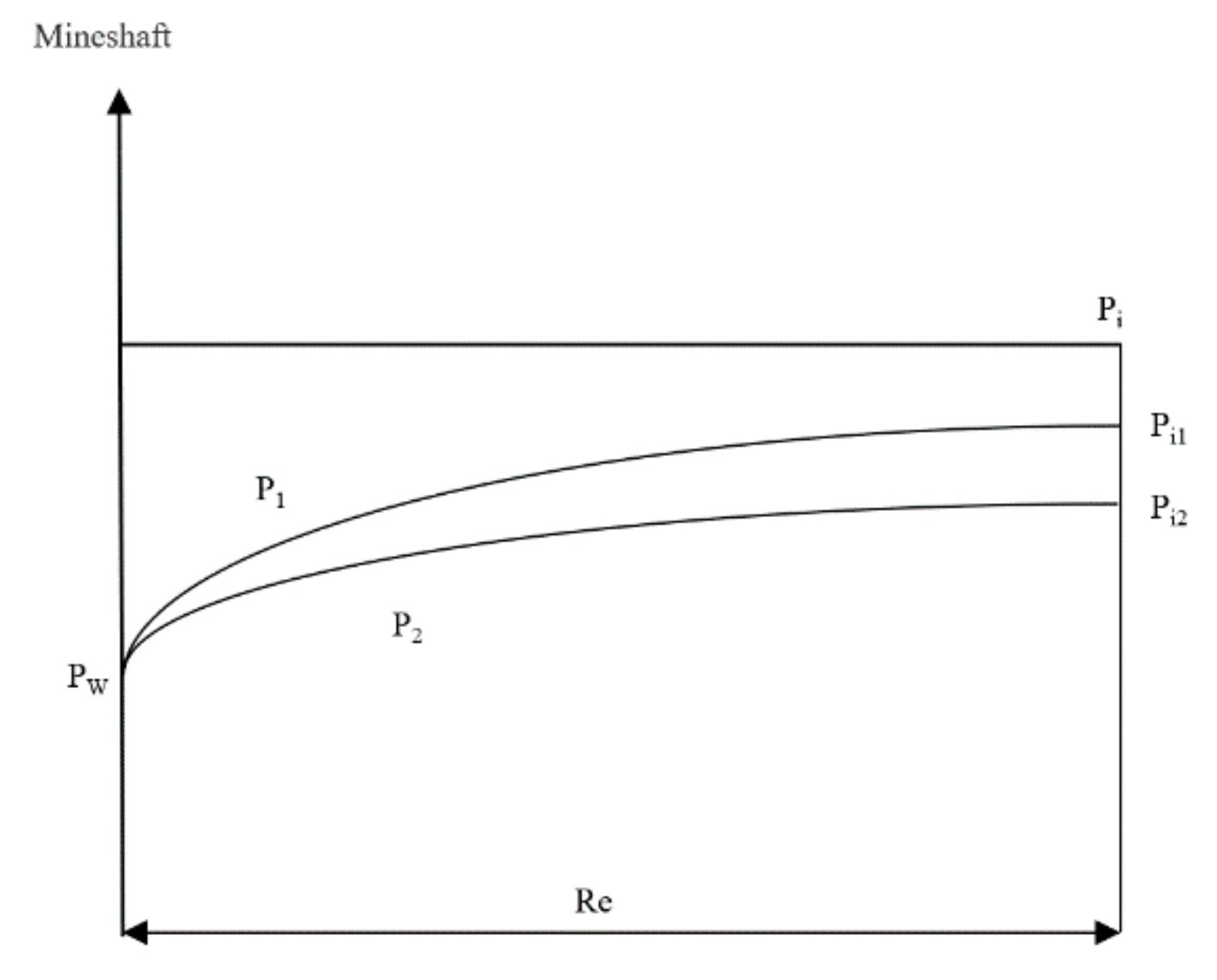
(3) After the pressure reaches the outer boundary, consider the t_2:+Δt time period, and the pressure at the outer boundary changes from P_i1→P_i2 (see Figure 3).

Formation pressure P₁ distribution at time t_2::

$$p_1=\frac{p_{i1}-p_w}{\ln \frac{r_e}{r_w}}\ln r+\frac{p_w\ln r_e-p_{i1}\ln r_w}{\ln \frac{r_e}{r_w}}$$

(24)

Distribution of formation pressure P₂ at time t_2:+Δt:

$$p_2=\frac{p_{i2}-p_w}{\ln \frac{r_e}{r_w}}\ln r+\frac{p_w\ln r_e-p_{i2}\ln r_w}{\ln \frac{r_e}{r_w}}$$

(25)

The yield calculation formula becomes:

$$q_2=\frac{2\pi kh(p_{i2}-p_w)}{\mu \ln \frac{r_e}{r_w}}=\frac{1-p_{i2D}}{\ln r_{eD}}$$

(26)

The mass conservation equation after the pressure wave reaches the boundary:

$$q_2\Delta t={{\displaystyle \sum \{\pi h[(r+\Delta r)}}^2-r^2]\varphi C_t\Delta p\}=2\pi h\varphi C_t{\displaystyle {\int }_{r_w}^{r_e}r(p_1-p_2)dr}$$

(27)

Substitute (24)–(26) into (27) to solve P_i2 (the initial value of P_i1 is P_i):

$$p_{i2D}=\frac{\Delta t_D+[\frac{1}{2}{r}_{eD}^2\ln r_{eD}-\frac{1}{4}(r_{eD}^2-1)]p_{i1D}}{\Delta t_D+\frac{1}{2}{r}_{eD}^2\ln r_{eD}-\frac{1}{4}(r_{eD}^2-1)}$$

(28)

Equation (28) gave the outer dimensionless boundary pressure. Equation (26) gave the dimensionless wellbore production. They comprised a nonlinear solution of the moving boundary nonlinear equation.

For the constant pressure outer boundary, if the sweep radius is greater than the outer boundary radius, the sweep radius is taken as the outer boundary radius.

For the closed boundary, if the sweep radius is greater than the outer boundary radius, the outer boundary radius will not change, but the pressure at the outer boundary will change.

2.2. Non-Darcy Flow of Low-Permeability Reservoir

2.2.1. Mathematical Model

①

The oil reservoir is isotropic and homogeneous with circular, uniform thickness, closed top and bottom, and uniform original formation pressure;

②

The fluid is single-phase and micro-compressible, and the seepage flow is under constant temperature without physical and chemical changes and satisfies Darcy’s law; permeability, porosity, compressibility, and viscosity, etc., are all constants and do not change with time or pressure;

③

The influence of gravity is ignored, and the pressure gradient is small.

Considering a constant pressure production well in the center of a circular homogeneous area, the flow equation of the flow zone in a low-permeability reservoir is as follows:

$$\frac{1}{r}\frac{\partial }{\partial r}[r(\frac{\partial p}{\partial r}-G)]=\frac{\mu \varphi C_t}{k}\frac{\partial p}{\partial t}$$

(29)

Internal boundary conditions of constant pressure:

$$p{\left|\right.}_{r_w}=p_w$$

(30)

Infinite outer boundary:

$$\underset{r\to \infty }{\lim }p=p_i$$

(31)

Constant pressure outer boundary:

$$p{\left|\right.}_{r_e}=p_i$$

(32)

Closed outer boundary:

$$p\prime {\left|\right.}_{r_e}=0$$

(33)

2.2.2. Moving Boundary Nonlinear Equation

The steady-state pressure equation in the flow zone:

$$\frac{1}{r}\frac{\partial }{\partial r}[r(\frac{\partial p}{\partial r}-G)]=0$$

(34)

Integral solution to obtain the formation pressure distribution:

$$p=c_1\ln r+Gr+c_2$$

(35)

c₁, c₂ is the integral constant.

Formation pressure P₁ within the range of moving boundary r₁ at time t:

$$p_1=\frac{p_i-p_w-G(r_1-r_w)}{\ln \frac{r_1}{r_w}}\ln r+Gr+\frac{(p_w-G{r}_w)\ln r_1-(p_i-G{r}_1)\ln r_w}{\ln \frac{r_1}{r_w}}$$

(36)

Formation pressure P₂ in the range of moving boundary r₂ at time t_2:+Δt:

$$p_2=\frac{p_i-p_w-G(r_2-r_w)}{\ln \frac{r_2}{r_w}}\ln r+Gr+\frac{(p_w-G{r}_w)\ln r_2-(p_i-G{r}_2)\ln r_w}{\ln \frac{r_2}{r_w}}$$

(37)

Dimensionless bottom-hole production calculation formula:

$$q_D=\frac{\mu q}{172.8\pi kh(p_i-p_w)}=\frac{1+G_D-G_D\cdot r_{1D}}{\ln r_{1D}}$$

(38)

Among them: G_D is the dimensionless starting pressure gradient, dimensionless,

$$G_D=\frac{G{r}_w}{p_i-p_w}$$

As r increases, the yield gradually decreases.

Formation quality conservation equation in Δt time:

$$\begin{array}{l}{q}_1\Delta t={{\displaystyle \sum \{\pi h[(r+\Delta r)}}^2-r^2]\varphi C_t\Delta p\}\\ =172.8\pi h\varphi C_t[{\displaystyle {\int }_{r_w}^{r_1}r(p_1-p_2)dr}+{\displaystyle {\int }_{r_1}^{r_2}r(p_i-p_2)dr}]\end{array}$$

(39)

Of which:

$${\displaystyle {\int }_{r_w}^{r_1}r(p_1-p_2)dr}=A{\displaystyle {\int }_{r_w}^{r_1}r\ln rdr}-A\ln r_w{\displaystyle {\int }_{r_w}^{r_1}rdr}$$

(40)

$$\begin{array}{l}{\displaystyle {\int }_{r_1}^{r_2}r(p_i-p_2)dr}=\frac{(p_i-p_w+G{r}_w)\ln r_2-G{r}_2\ln r_w}{\ln \frac{r_2}{r_w}}{\displaystyle {\int }_{r_1}^{r_2}rdr}\\ -\frac{(p_i-p_w+G{r}_w)-G{r}_2}{\ln \frac{r_2}{r_w}}{\displaystyle {\int }_{r_1}^{r_2}r\ln rdr}-G{\displaystyle {\int }_{r_1}^{r_2}{r}^{2}dr}\end{array}$$

(41)

Substituting (40) and (41) into (39), we obtain:

$$4\frac{1+G_D-G_D\cdot r_{1D}}{\ln r_{1D}}\cdot \Delta t_D=\frac{r_{1D}^2-1}{\ln r_{1D}}-2+G_D[\frac{(r_{1D}^2-1)\cdot (1-r_{1D})}{\ln r_{1D}}+\frac{2}{3}(r_{1D}^3-1)]$$

(42)

$$\begin{array}{l}(r_{2D}^2-1)\ln r_{1D}-(r_{1D}^2-1)\ln r_{2D}+G_D[(r_{2D}^2-1)\cdot (1-r_{2D})\cdot \ln r_{1D}-(r_{1D}^2-1)\cdot (1-r_{1D})\cdot \ln r_{2D}]\\ +\frac{2}{3}{G}_D(r_{2D}^3-r_{1D}^3)\cdot \ln r_{1D}\cdot \ln r_{2D}=4(1+G_D-G_D{r}_{2D})\Delta t_D\cdot \ln r_{1D}\end{array}$$

(43)

After the pressure reaches the outer boundary, consider the time period t₂→t₂:+Δt, and the pressure at the outer boundary starts from P_i1→P_i2.

Distribution of formation pressure P₁ at time t₂:

$$p_1=\frac{p_{i1}-p_w-G(r_e-r_w)}{\ln \frac{r_e}{r_w}}\ln r+Gr+\frac{(p_w-G{r}_w)\ln r_e-(p_{i1}-G{r}_e)\ln r_w}{\ln \frac{r_e}{r_w}}$$

(44)

Distribution of formation pressure P₂ at time t₂:+Δt:

$$p_2=\frac{p_{i2}-p_w-G(r_e-r_w)}{\ln \frac{r_e}{r_w}}\ln r+Gr+\frac{(p_w-G{r}_w)\ln r_e-(p_{i2}-G{r}_e)\ln r_w}{\ln \frac{r_e}{r_w}}$$

(45)

The yield calculation formula becomes:

$$q_D=\frac{\mu q}{172.8\pi kh(p_i-p_w)}=\frac{1-p_{i2\mathrm{D}}-G_D(r_{eD}-1)}{\ln r_{eD}}$$

(46)

When the pressure wave reaches the boundary, the mass conservation equation can be expressed as:

$$q_1\Delta t={{\displaystyle \sum \{\pi h[(r+\Delta r)}}^2-r^2]\varphi C_t\Delta p\}=172.8\pi h\varphi C_t{\displaystyle {\int }_{r_w}^{r_{\mathrm{e}}}r(p_1-p_2)dr}$$

(47)

Substitute Equations (44)–(46) into Equation (47) to solve for p_i2D (p_i1D initial value is p_i).

$$p_{i2\mathrm{D}}=\frac{p_{i1\mathrm{D}}[\frac{1}{2}{r}_{eD}^2\ln r_{eD}-\frac{1}{4}(r_{eD}^2-1)]+[1-G_D(r_{eD}-1)]\Delta t_D}{\frac{1}{2}{r}_{eD}^2\ln r_{eD}-\frac{1}{4}(r_{eD}^2-1)+\Delta t_D}$$

(48)

Equations (42), (43) and (48) are made up of the nonlinear model of the low-permeability reservoir.

Similarly, for the external boundary with constant pressure, if the sweep radius is larger than the outer boundary radius, the sweep radius is taken as the outer boundary radius. For the closed boundary, if the sweep radius is greater than the outer boundary radius, the outer boundary radius will not change, but the pressure at the outer boundary will change. The nonlinear solution calculating process of the low-permeability reservoir is presented below.

Step1: Solving r_1D by Equation (42). Taking r_1D as the initial value, solving q_D by Equation (38).

①

If close boundary

Step2: Compared r_1D with r_eD.

If r_1D < r_eD, solving r_2D by Equation (42).Taking r_2D replace r_1D, solving q_D by Equation (37). Repeat step2.

If r_1D f r_eD, solving p_i2D by Equation (48). Solving q_D by Equation (46), calculation terminated.

②

If stable boundary

Step2: Compared r_1D with r_eD.

If r_1D < r_eD, solving r_2D by Equation (42).Taking r_2D replace r_1D, solving q_D by Equation (37). Repeat step2.

If r_1D f r_eD, taking p_i2D = 0(outer boundary pressure is pi). Solving q_D by Equation (46), calculation terminated.

③

If infinite boundary

Step2: Solving r_2D by Equation (42).Taking r_2D replace r_1D, solving q_D by Equation (38). Repeat step2.

3. Results and Error Analysis

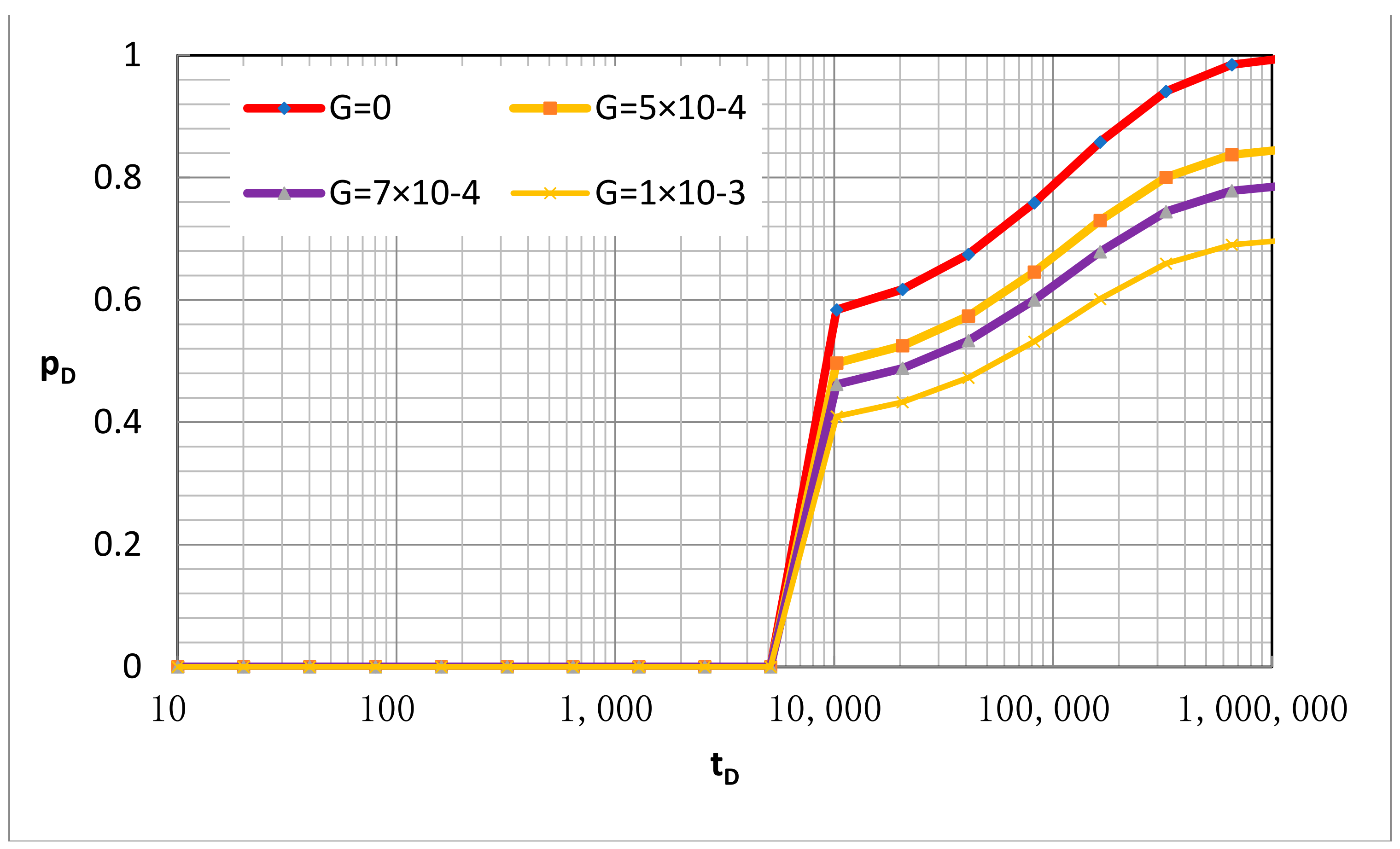
Figure 4 shows the variation curve of the outer boundary pressure of a closed reservoir under different start-up pressure gradients.

According to the established nonlinear calculation model of the outer boundary of the low-permeability reservoir, the production decline curve of the low-permeability reservoir with different outer boundary conditions under constant flow pressure can be obtained.

Based on the seepage theory, the analytical solution of the radial flow unstable seepage model in Laplace space is as follows:

Infinite outer boundary:

$$q_D=\frac{K_1(\sqrt{z})}{\sqrt{z}{K}_0(\sqrt{z})}$$

(49)

Closed outer boundary:

$$q_D=-\frac{1}{\sqrt{z}}\frac{K_1(\sqrt{z}\cdot r_{eD})I_1(\sqrt{z})-I_1(\sqrt{z}\cdot r_{eD})K_1(\sqrt{z})}{I_0(\sqrt{z})K_1(\sqrt{z}\cdot r_{eD})+I_1(\sqrt{z}\cdot r_{eD})K_0(\sqrt{z})}$$

(50)

Constant pressure outer boundary:

$$q_D=-\frac{1}{\sqrt{z}}\frac{K_0(\sqrt{z}\cdot r_{eD})I_1(\sqrt{z})-I_0(\sqrt{z}\cdot r_{eD})K_1(\sqrt{z})}{K_0(\sqrt{z}\cdot r_{eD})I_0(\sqrt{z})-I_0(\sqrt{z}\cdot r_{eD})K_0(\sqrt{z})}$$

(51)

The analytical solution could be solved by Stehfest’s numerical inversion [23]. Comparing the analytical solution with nonlinear solution, the relative error is calculated by the following formula.

$$\delta =\frac{q_{as}-q_{ns}}{q_{as}}\times 100\%$$

(52)

Among them:

q_as is an analytical solution, calculated by Equations (49)–(52);

q_ns is a nonlinear solution;

δ is relative error.

Table 1. Comparison of calculated results under infinite boundary.

Time	qas	qns	δ (%)	Time	qas	qns	δ (%)
10	0.534	0.526	1.48	384	0.284	0.292	–2.94
15	0.489	0.479	2.00	577	0.269	0.278	–3.45
23	0.450	0.443	1.74	865	0.255	0.265	–3.90
34	0.417	0.412	1.16	1297	0.243	0.254	–4.30
51	0.387	0.386	0.43	1946	0.232	0.243	–4.64
76	0.361	0.363	–0.32	2919	0.222	0.233	–4.95
114	0.339	0.342	–1.06	4379	0.213	0.224	–5.21
171	0.318	0.324	–1.75	6568	0.204	0.215	–5.45
256	0.300	0.307	–2.38	9853	0.196	0.207	–5.65

,

Table 2. Comparison of calculated results under stable boundary.

Time	qas	qns	δ (%)	Time	qas	qns	δ (%)
10	0.534	0.526	1.48	384	0.284	0.292	–2.94
15	0.489	0.479	2.00	577	0.269	0.278	–3.45
23	0.450	0.443	1.74	865	0.255	0.265	–3.90
34	0.417	0.412	1.16	1297	0.243	0.254	–4.28
51	0.387	0.386	0.43	1946	0.233	0.243	–4.44
76	0.361	0.363	–0.32	2919	0.224	0.233	–3.88
114	0.339	0.342	–1.06	4379	0.219	0.224	–2.01
171	0.318	0.324	–1.75	6568	0.218	0.217	0.18
256	0.300	0.307	–2.38	9853	0.217	0.217	0.00

and

Table 3. Comparison of calculated results under close boundary.

Time	qas	qns	δ (%)	Time	qas	qns	δ (%)
10	0.534	0.526	1.48	384	0.284	0.292	–2.94
15	0.489	0.479	2.00	577	0.269	0.278	–3.45
23	0.450	0.443	1.74	865	0.255	0.265	–3.90
34	0.417	0.412	1.16	1297	0.243	0.254	–4.31
51	0.387	0.386	0.43	1946	0.232	0.243	–4.88
76	0.361	0.363	–0.32	2919	0.219	0.233	–6.37
114	0.339	0.342	–1.06	4379	0.203	0.224	–10.23
171	0.318	0.324	–1.75	6568	0.181	0.161	11.06
256	0.300	0.307	–2.38	9853	0.153	0.151	1.51

show the comparison results of the nonlinear solution and the analytical solution under different external boundary conditions. The error of the nonlinear solution and the analytical solution is very small, which fully meets the calculation accuracy requirements.

4. Results and Discussion

4.1. Propagation Mechanism of Moving Boundary

The moving boundary propagation mechanism is a difficult point in the study of low-permeability reservoirs, and the pressure sweep radius is the core indicator of low-permeability reservoir development technology policy formulation. At present, mainstream commercial numerical simulation software uses the Darcy flow method to simulate the development of low-permeability reservoirs. Many experts and scholars adopt a step-by-step numerical simulation method, which firstly determines the flowable grid iteratively, and then performs the simulation calculation on the flowable grid. When the mainstream nonuniform grid is used to perform step-by-step simulation calculations, the calculation error will be significant if the grid is too large.

The model in this study can accurately calculate the low-permeability reservoir sweep radius, and the pressure sweep radius with different start-up pressure gradients was calculated. A convenient formula for calculating the swept radius under different starting pressure gradients must be established, and it can provide theoretical guidance for the formulation of low-permeability reservoir development technology policies.

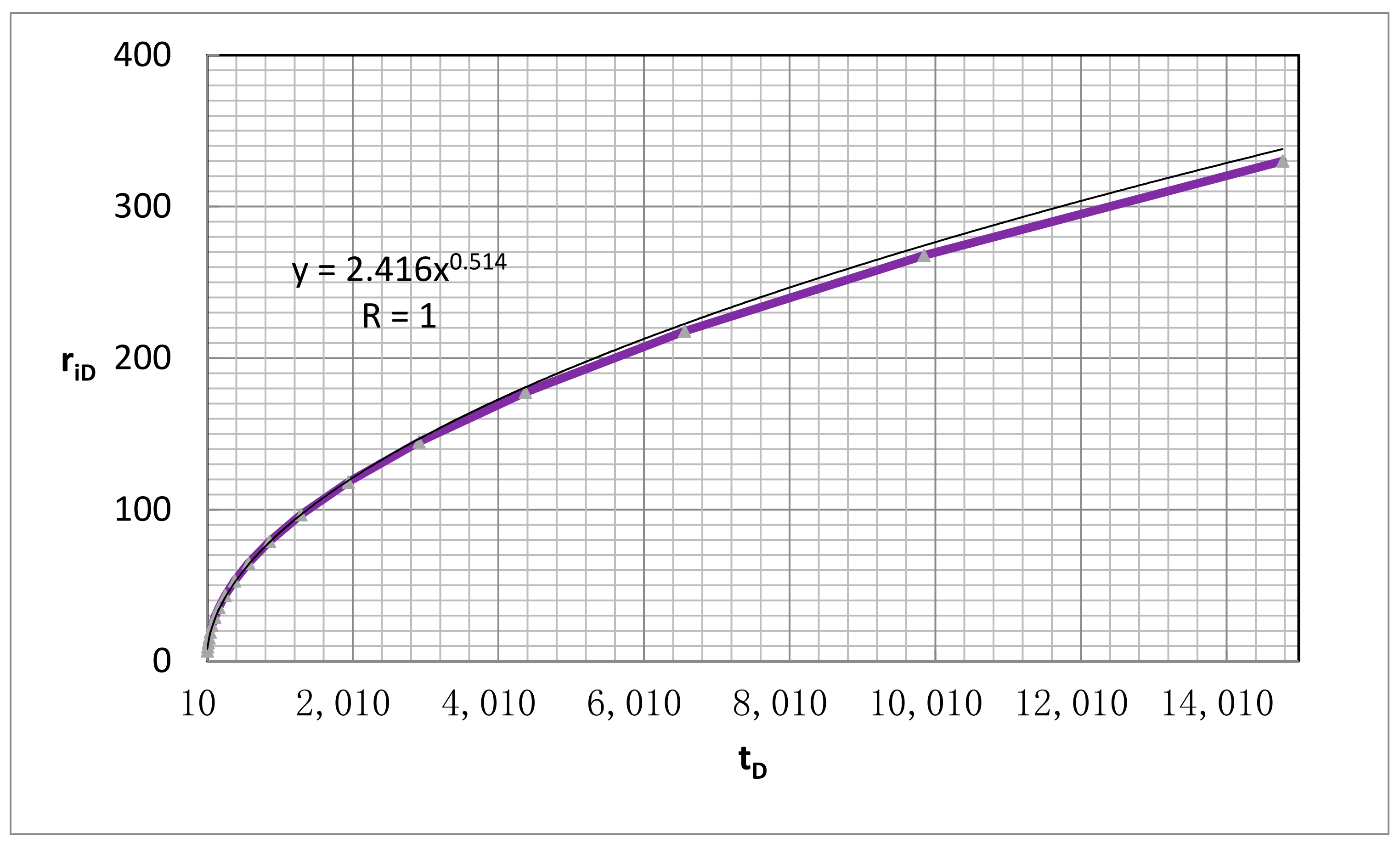
Different models are used for fitting. When a power function is used for fitting (Figure 5), the correlation coefficient is the greatest (R = 0.999). Therefore, it is reasonable to use the power function model to fit. Calculate the curve of the sweep radius versus time under different starting pressure gradients G_D, and, respectively, fit a and b under different starting pressure gradients.

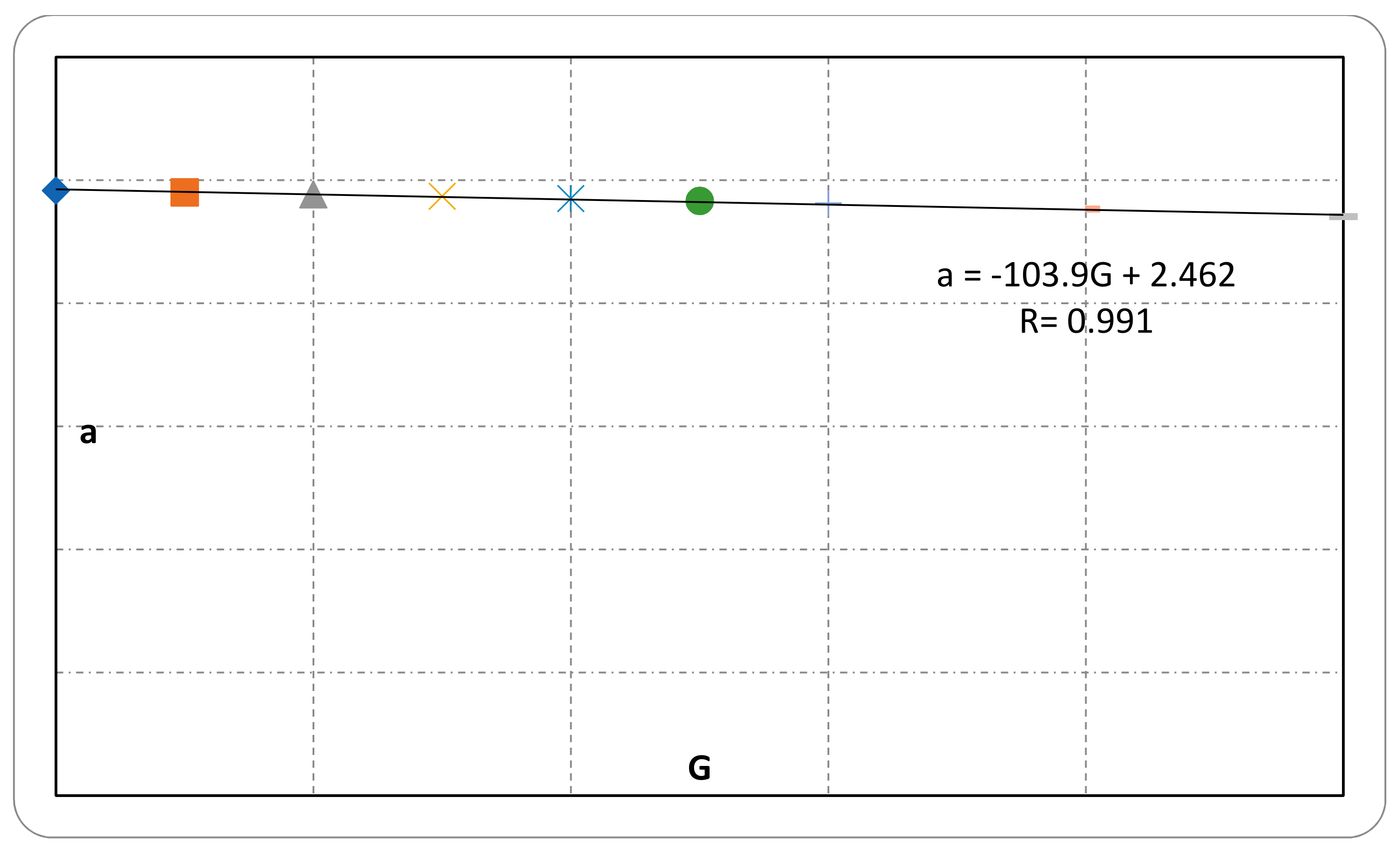
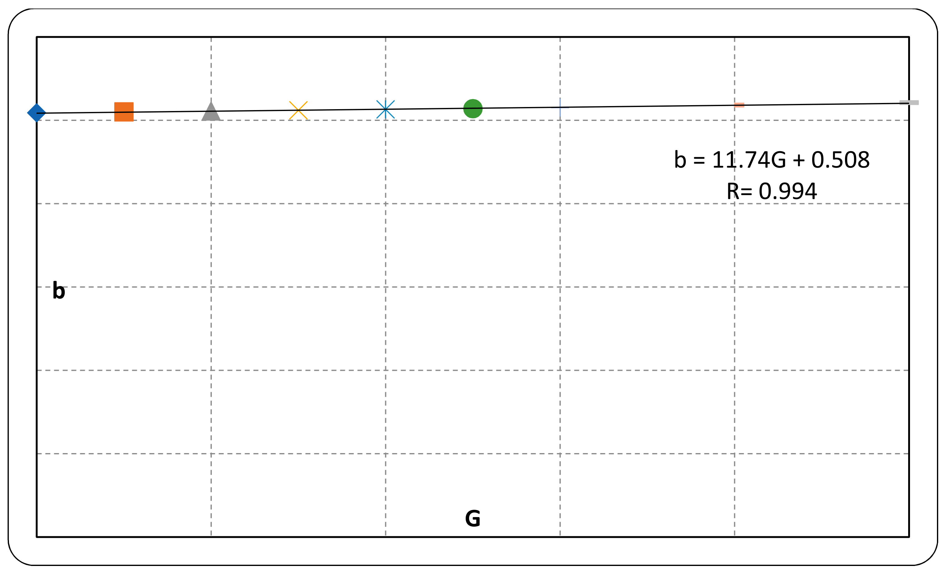
The coefficient a and exponent b linear fitting curves were drawn under different starting pressure gradients (Figure 6 and Figure 7). The fitting results indicate that the linear model can reach a higher fitting accuracy (

Table 4. Comparison of calculating results under a closed boundary.

Starting Pressure Gradient	a	b	Correlation Coefficient
0	2.457	0.509	0.998
0.0001	2.450	0.510	0.998
0.0002	2.442	0.511	0.998
0.0003	2.434	0.512	0.998
0.0004	2.425	0.513	0.998
0.0005	2.416	0.514	0.998
0.0006	2.405	0.515	0.998
0.0008	2.381	0.518	0.998
0.001	2.351	0.521	0.998

, R exceeds 0.998), and the linear model can be used for an approximate calculation.

By substituting the power function, the calculation formula of the sweep radius under constant flow pressure conditions of a low-permeability reservoir can be obtained:

$$r_{iD}=(2.462-103.9\cdot G_D)\cdot t_D^{11.74\cdot G_D+0.508}$$

(53)

The sweep radius is a function of a dimensionless start-up pressure gradient and dimensionless time. The propagation law of the sweep radius in a low-permeability reservoir can be determined through dimensionless formula conversion, which can provide theoretical guidance for well spacing and well pattern design in a low-permeability reservoir.

4.2. Analysis of Production Decline

The production decline curve reflects the stable production situation of the reservoir. Generally, the production decline curve generated by statistical field data is compared with the theoretical curve chart to evaluate the reservoir development effect. According to the established nonlinear calculation model of the outer boundary of a low-permeability reservoir, the production decline curve chart of a low-permeability reservoir with different outer boundary conditions under constant flow pressure can be obtained.

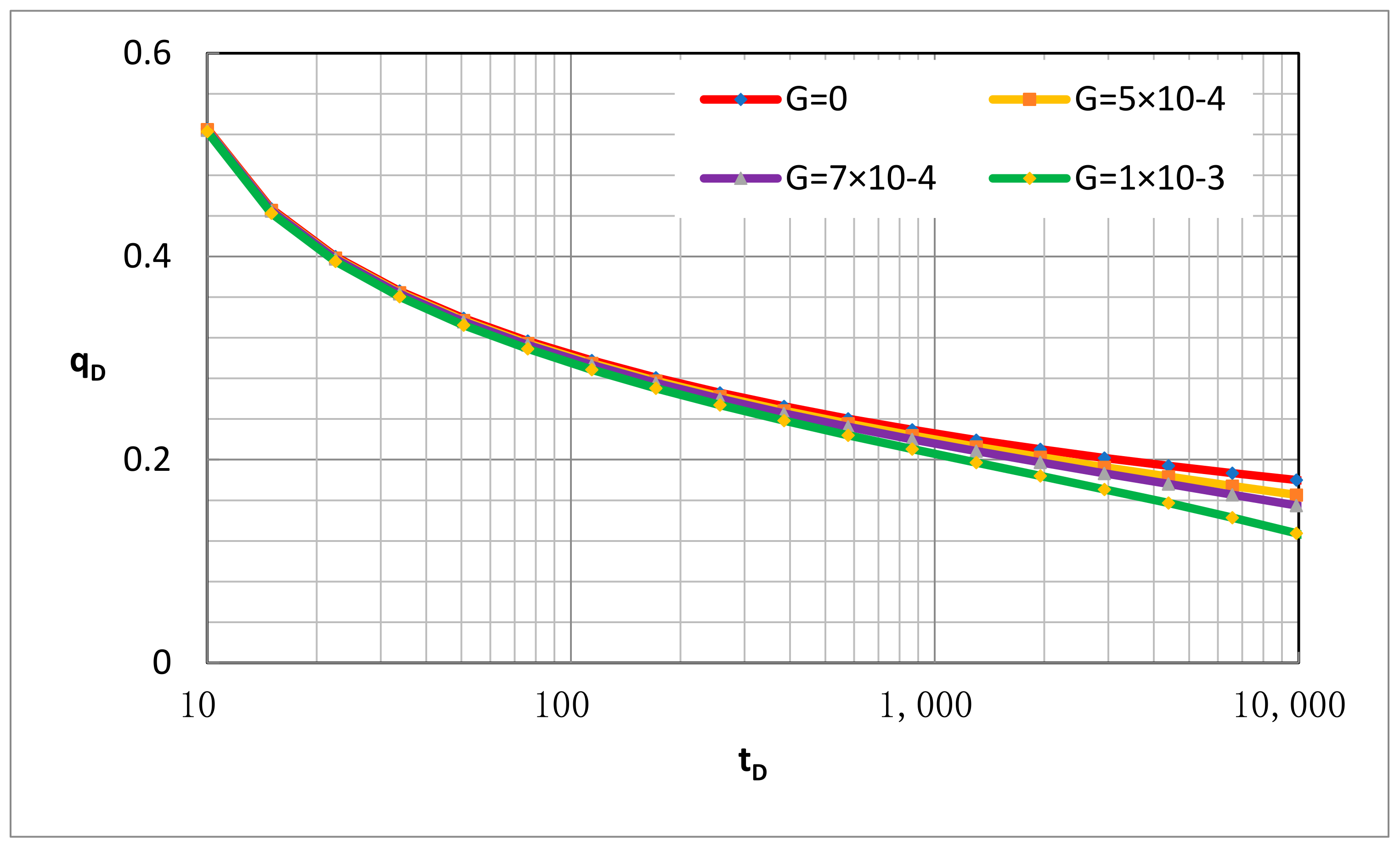
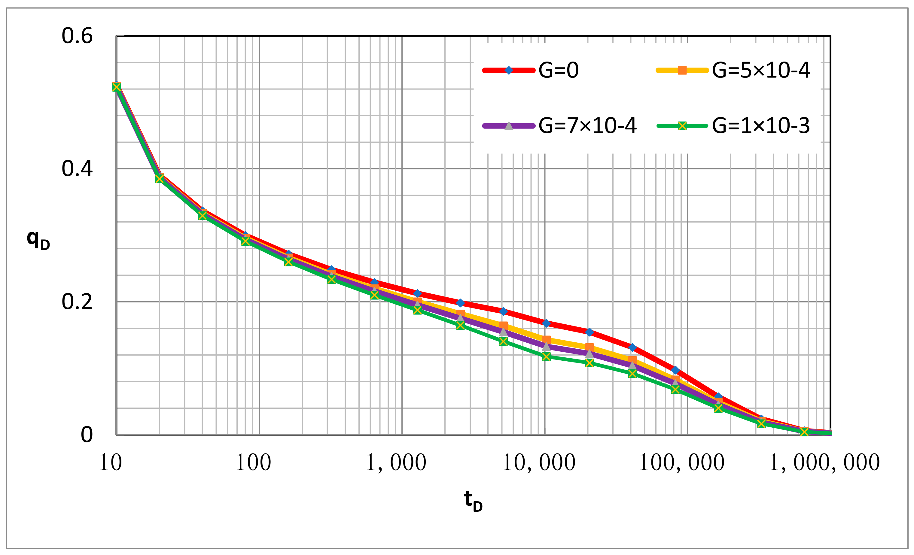
For infinite reservoirs, the boundary cannot be detected within the calculation time, so the key factor affecting the production decline curve is only the dimensionless start-up pressure gradient. For infinite reservoirs, the larger the start-up pressure gradient is, the faster the production will decline (Figure 8).

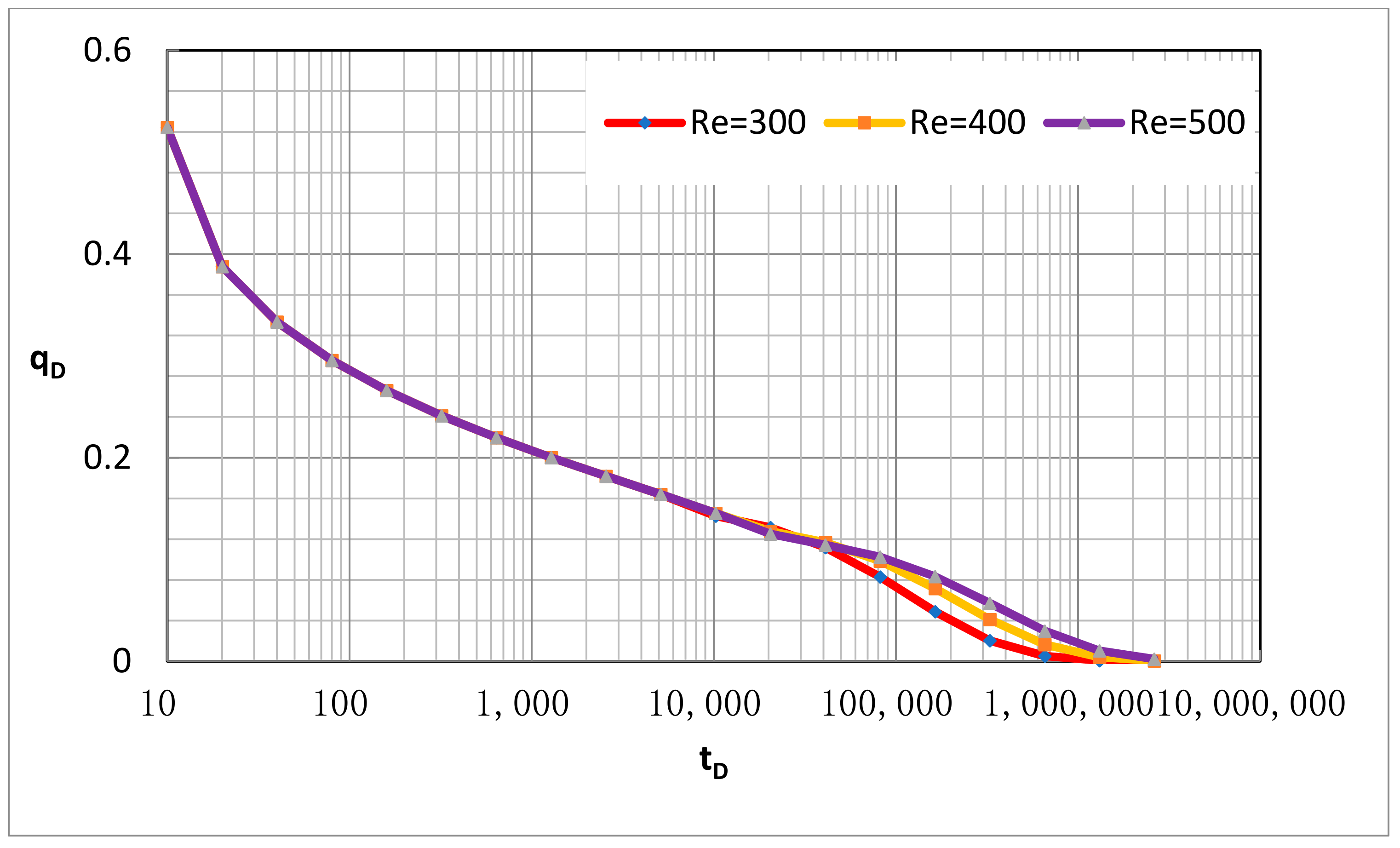
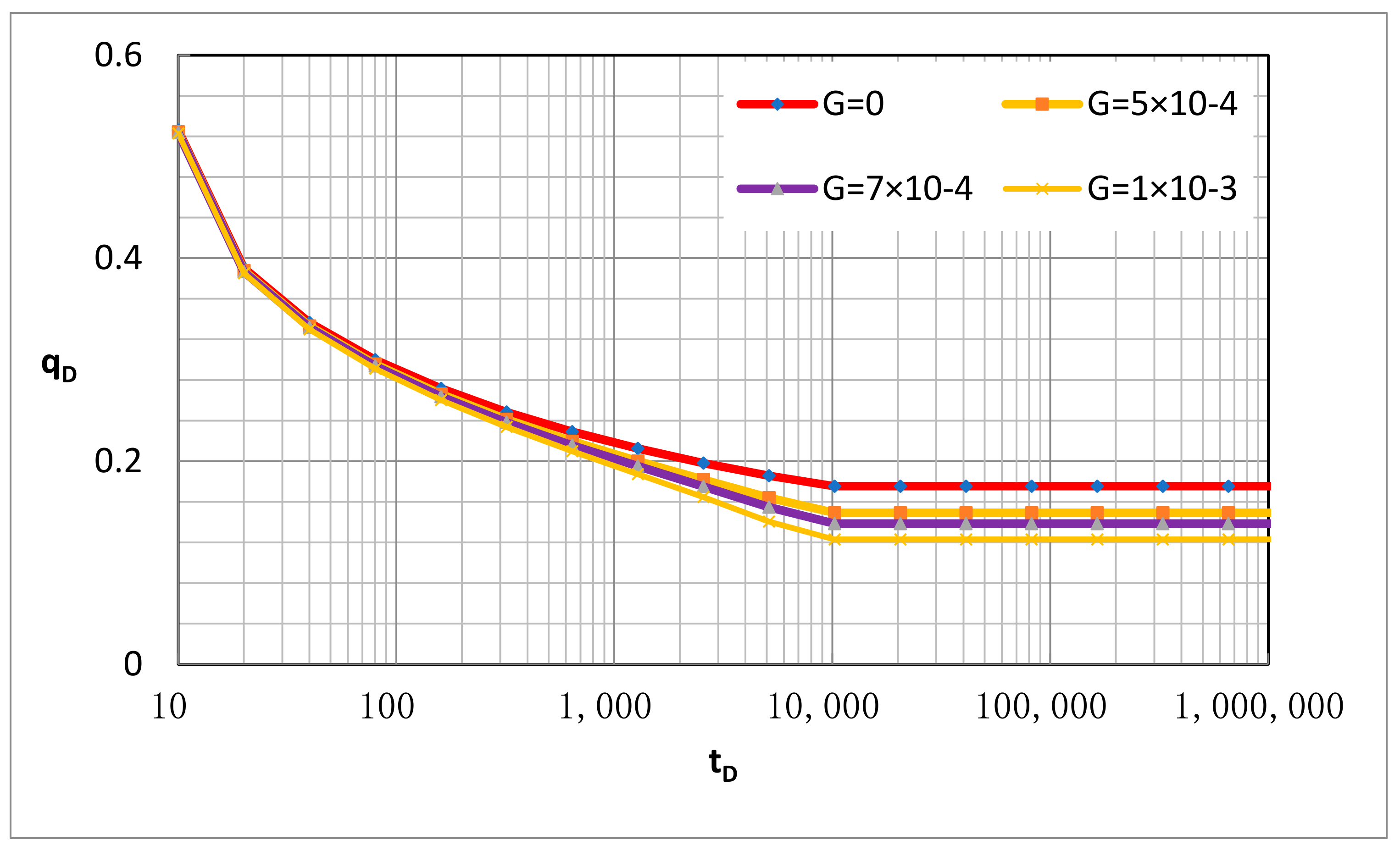
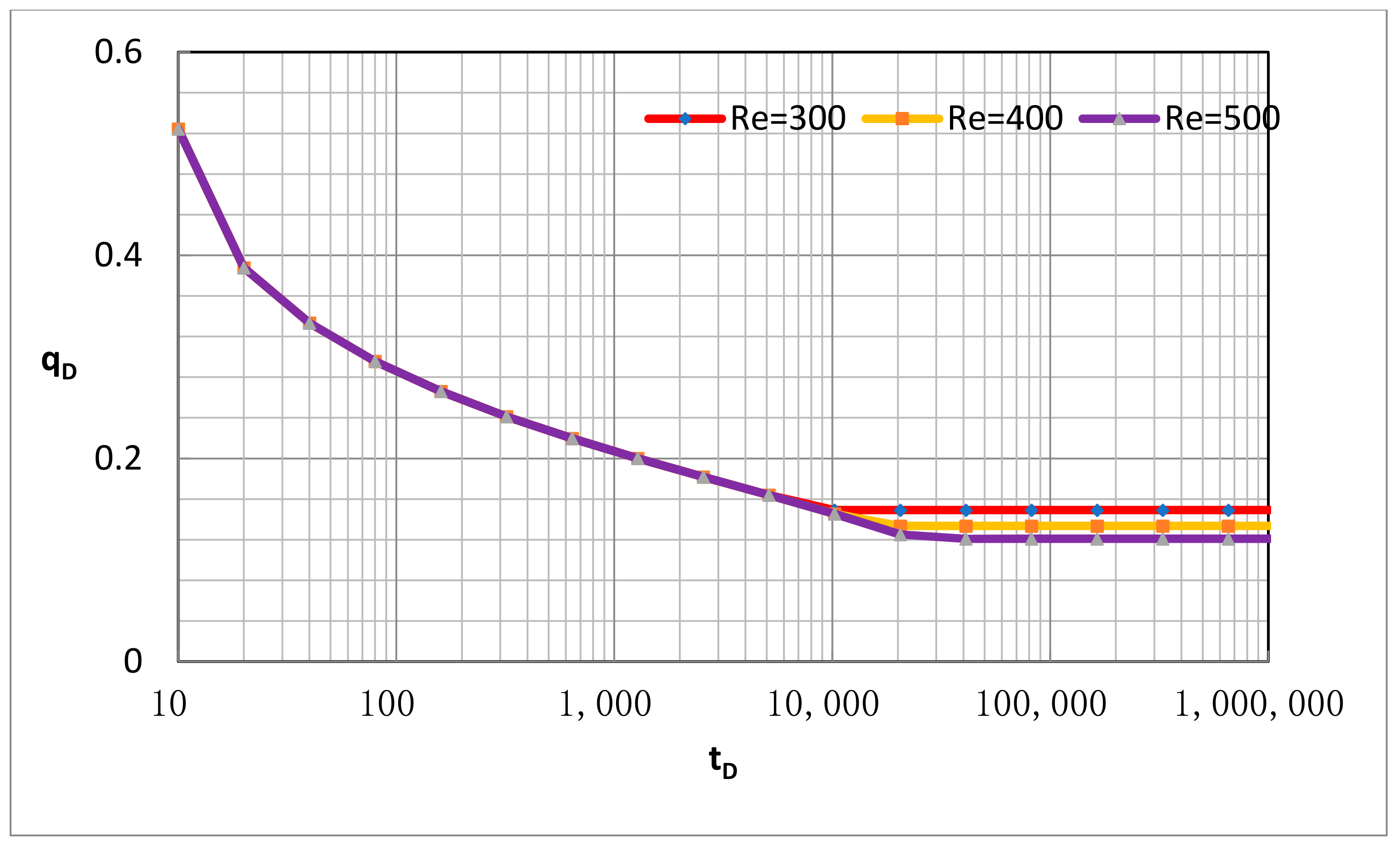
For closed outer boundary reservoirs, both dimensionless start-up pressure gradient and outer boundary radius will affect the shape of the production decline curve (Figure 9 and Figure 10). The starting pressure gradient affects the slope of the curve. The larger the dimensionless starting pressure gradient is, the faster the output will decline; the smaller the outer boundary radius is, the faster the output will be depleted.

For constant pressure boundary reservoirs, the larger the starting pressure gradient is, the faster the production will decline. After the final production is stable, the larger the starting pressure gradient, the lower the production (Figure 11 and Figure 12).

4.3. Recovery Factor of Low-Permeability Reservoir

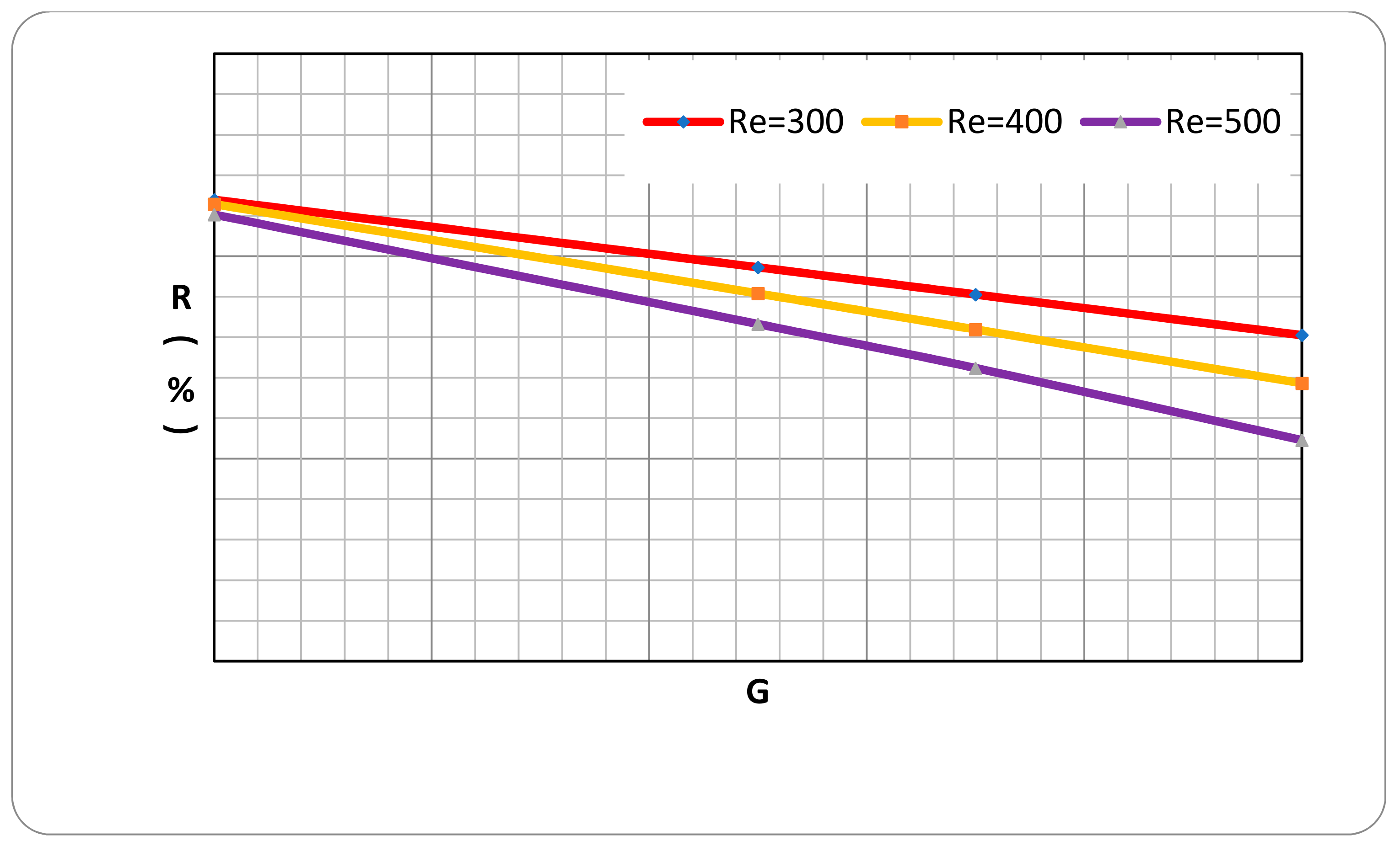
The recovery factor determines the economic and technical limits of low-permeability reservoirs and is the core indicator of the low-permeability reservoir development program.

At present, empirical formula methods, field statistics methods, numerical simulation methods, and theoretical derivation methods, etc., are mainly used for calculating the recovery factor of low-permeability oil reservoirs. In this study, the production curve chart of closed reservoirs under different starting pressure gradients has been established. Therefore, the cumulative production can be obtained by numerical calculation methods, and the recovery factor of low-permeability reservoirs can be calculated using the cumulative production. According to the closed-boundary production decline curve, the cumulative production is approximated by the numerical integration method.

$$N_p=\frac{q_1{t}_2-\frac{1}{2}(q_2+q_1)t_1}{t_2-t_1}{t}_1+{\displaystyle \sum _{i=2}^n[\frac{1}{2}(t_i-t_{i-1})\cdot (q_i+q_{i-1})]}+\frac{1}{2}{q}_n^2\frac{t_n-t_{n-1}}{q_{n-1}-q_n}$$

(54)

Among them, t_i and q_i are output decline curve data.

Then, the cumulative production and geology reserves can be used to calculate the recovery factor and the oil recovery factor under different outer boundary radii and start-up pressure gradients and draw the low-permeability reservoir recovery factor map (Figure 13).

For a given starting pressure gradient and well spacing, the oil recovery factor can be queried from the chart.

5. Conclusions

(1)

Based on the steady-state sequential substitution method of the seepage mechanics theory, the moving boundary nonlinear equations of the infinite outer boundary, constant pressure outer boundary and closed outer boundary in production with constant flow pressure of a homogeneous reservoir under Darcy‘s seepage condition are derived, respectively. The nonlinear equation is solved by the quasi-Newton method, and the obtained nonlinear solution is compared with the analytical solution. The comparison shows that the method has high accuracy and can be used to solve the problem of unstable seepage. The research in this paper provides a third method for solving the oil and gas seepage equation, which is different from the analytical solution and the numerical solution and provides a new method for the solution of linear partial differential equations.

(2)

Based on the quasi-linear flow equations of low-permeability reservoirs, the moving boundary nonlinear equations with an infinite outer boundary, constant pressure outer boundary, and closed outer boundary are deduced during production with constant flow pressure in low-permeability reservoirs, and production decline charts of different outer boundaries are established.

(3)

Based on the nonlinear equation of the moving boundary of the low-permeability reservoir, the calculation formula of the sweep radius of the low-permeability reservoir was established, and the calculation chart of the recovery factor was drawn, which can provide a theoretical reference for the formulation of low-permeability reservoir development technology policies.

References

- Darcy, H. Les Fontaines Publiques de La Ville de Dijon; Dalmont: Paris, France, 1865. [Google Scholar]
- Bear, J. Dynamic of Fluid in Porous Media; Elsevier: Alpharetta, GA, USA, 1972; pp. 127–128. [Google Scholar]
- Prada, A.; Civam, F. Modification of Darcy’s Law for the threshold pressure gradient. J. Pet. Sci. Eng. 1999, 22, 237–240. [Google Scholar] [CrossRef]
- Civan, F. Porous Media Transport Phenomena; John Wiley & Sons Press: Hoboken, NJ, USA, 2011. [Google Scholar]
- Ding, J.; Yang, S.; Cao, T.; Wu, J. Dynamic threshold pressure gradient in tight gas reservoir and its influence on well productivity. Arab. J. Geosci. 2018, 11, 783. [Google Scholar] [CrossRef]
- Huang, Y. Nonlinear percolation feature in low permeability reservoir. Spec. Oil Gas Reserv. 1997, 4, 9–14. [Google Scholar]
- Dou, H.; Ma, S.; Zou, C.; Yao, S. Threshold pressure gradient of fluid flow through multi-porous media in low and extra-low permeability reservoirs. Sci. China Earth Sci. 2014, 57, 2808–2818. [Google Scholar] [CrossRef]
- Lu, C.; Wang, J.; Sun, Z. An experimental study on starting pressure gradient of fluids flow in low permeability sandstone porous media. Pet. Explor. Dev. 2002, 29, 86–89. [Google Scholar]
- Pascal, H. Nonsteady flow through porous media in the presence of a threshold gradient. Acta Mech. 1981, 39, 207–224. [Google Scholar] [CrossRef]
- Wu, Y.-S. Theoretical Studies of Non-Newtonian and Newtonian Fluid Flow through Porous Media; University of California: Berkeley, CA, USA, 1990. [Google Scholar]
- Wu, Y.S.; Pruess, K.; Witherspoon, P.A. Flow and displacement of Bingham Non-Newtonian fluids in porous media. SPE Reserv. Eng. 1993, 7, 369–376. [Google Scholar] [CrossRef] [Green Version]
- Feng, G.Q.; Liu, Q.G.; Shi, G.Z.; Lin, Z.H. An unsteady seepage flow model considering kickoff pressure gradient for low-permeability gas reservoirs. Pet. Explor. Dev. 2008, 35, 457–461. [Google Scholar] [CrossRef]
- Chen, M.; Rossen, W.; Yortsos, Y.C. The flow and displacement in porous media of fluids with yield stress. Chem. Eng. Sci. 2005, 60, 4183–4202. [Google Scholar] [CrossRef]
- Lu, J.; Dai, F.; Rahman, M.M.; Escobar, F.H. Boundary Dominated Flow in Low Permeability Reservoir with Threshold Pressure Gradient. ARPN J. Eng. Appl. Sci. 2017, 12, 6834–6843. [Google Scholar]
- Lu, J.; Shi, S.; Rahman, M.M. New mathematical models for production performance of a well producing at constant bottom hole pressure. Porous Media 2018, 9, 261–278. [Google Scholar]
- Yun, M.; Yu, B.; Cai, J. A fractal model for the starting pressure gradient for Bingham fluids in porous media. Int. J. Heat Mass Transf. 2008, 51, 1402–1408. [Google Scholar] [CrossRef]
- Yun, M.; Yu, B.; Lu, J.; Zheng, W. Fractal analysis of Herschel-Bulkley fluid flow in porous media. Int. J. Heat Mass Transf. 2010, 53, 3570–3574. [Google Scholar] [CrossRef]
- Xie, K.H.; Wang, K.; Wang, Y.L.; Li, C.X. Analytical solution for one-dimensional consolidation of clayey soils with a threshold gradient. Comput. Geotech. 2010, 37, 487–493. [Google Scholar] [CrossRef]
- Liu, W.; Yao, J.; Wang, Y. Exact analytical solutions of moving boundary problems of one-dimensional flow in semi-infinite long porous media with threshold pressure gradient. Int. J. Heat Mass Transf. 2012, 55, 6017–6022. [Google Scholar] [CrossRef]
- Wang, X.; Zhu, G.; Wang, L. Exact analytical solutions for moving boundary problems of one-dimensional flow in semi-infinite porous media with consideration of threshold pressure gradient. J. Hydrodyn. 2015, 27, 542–547. [Google Scholar] [CrossRef]
- Huang, Y.; Liu, G. A Rate Decline Model of Composite Reservoir with Threshold Pressure Gradient. In International Field Exploration and Development Conference; Springer: Singapore, 2020. [Google Scholar] [CrossRef]
- Van Poollen, H.K. Radius of drainage and stabilization-time equations. Oil Gas J. 1964, 62, 138. [Google Scholar]
- Stehfest, H. Numerical inversion of Laplace transforms algorithm. J. Assoc. Comput. Mach. 1979, 13, 47–49. [Google Scholar]
Figure 1.
Radial flow model.
Figure 2.
Reservoir pressure distribution before pressure arrived at the outer boundary.
Figure 3.
Reservoir pressure distribution after pressure arrived at the closed boundary.
Figure 4.
The law of pressure change at the outer boundary of a closed reservoir.
Figure 5.
Relationship between sweep radius and time in low-permeability reservoirs (G = 5 × 10⁻⁴).
Figure 6.
Relationship between coefficient a and the starting pressure gradient.
Figure 7.
Relationship between exponent b and the starting pressure gradient.
Figure 8.
Production decline curve plate of an infinite low-permeability reservoir.
Figure 9.
Production decline curve plate of closed boundary low-permeability reservoir under different starting pressure gradients.
Figure 10.
Production decline curve plate of closed boundary low-permeability reservoir with different outer boundary radii.
Figure 11.
Production decline curve of stable boundary low-permeability reservoir with different starting pressure gradients.
Figure 12.
Production decline curve of stable boundary low-permeability reservoir with different outer boundary radius.
Figure 13.
Recovery of a low-permeability reservoir with different starting pressure gradients and outer boundary radii.