
A Novel Hybrid Feature Selection Method for Day-Ahead Electricity Price Forecasting

 , , ,
, , ,  and
and 
Abstract
:1. Introduction
- A novel hybrid method based on elitist GA and tree based method for input FS in price prediction,
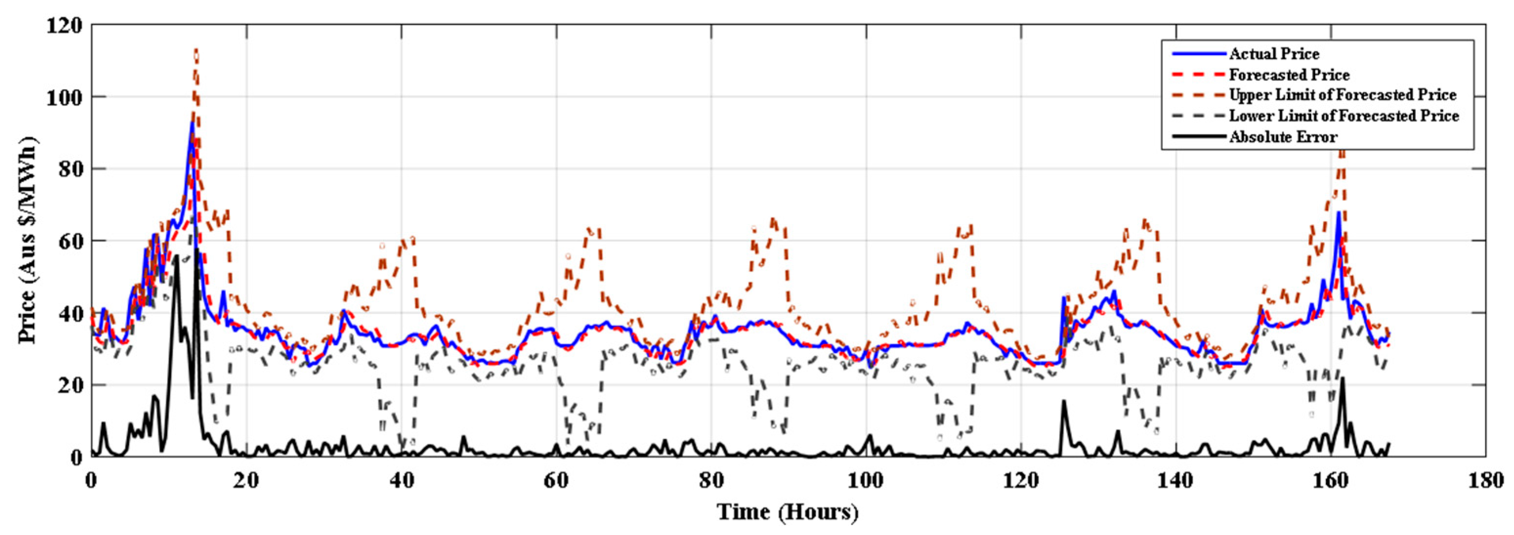
- Fixing the error margins during price prediction by applying the confidence interval, and
- Season-wise optimize FS to have a better forecasting accuracy.
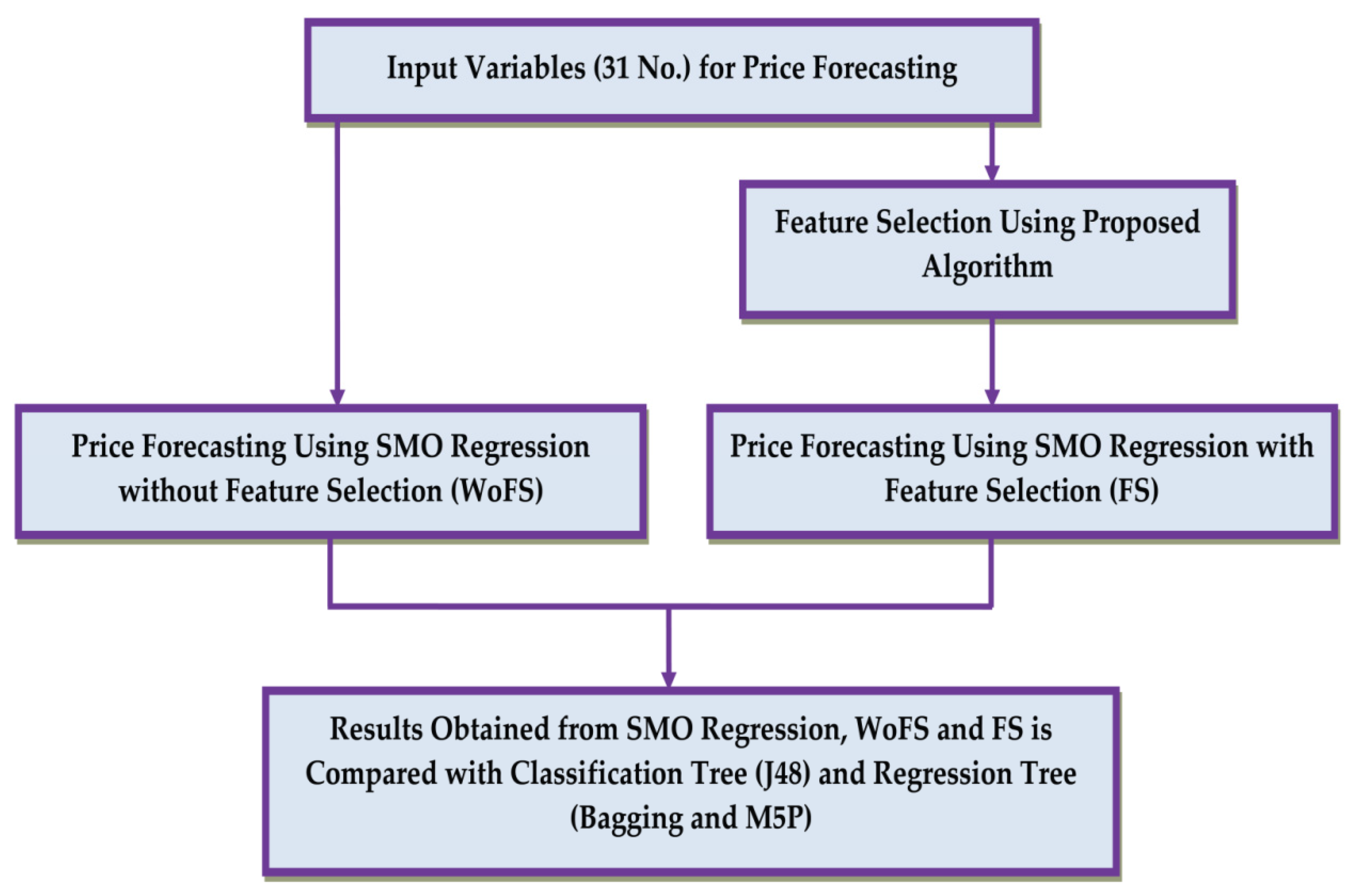
2. Proposed Methodology
3. Sequential Minimal Optimization (SMO) Regression Algorithm
3.1. Methodology
3.2. Calculation of SMO Regression
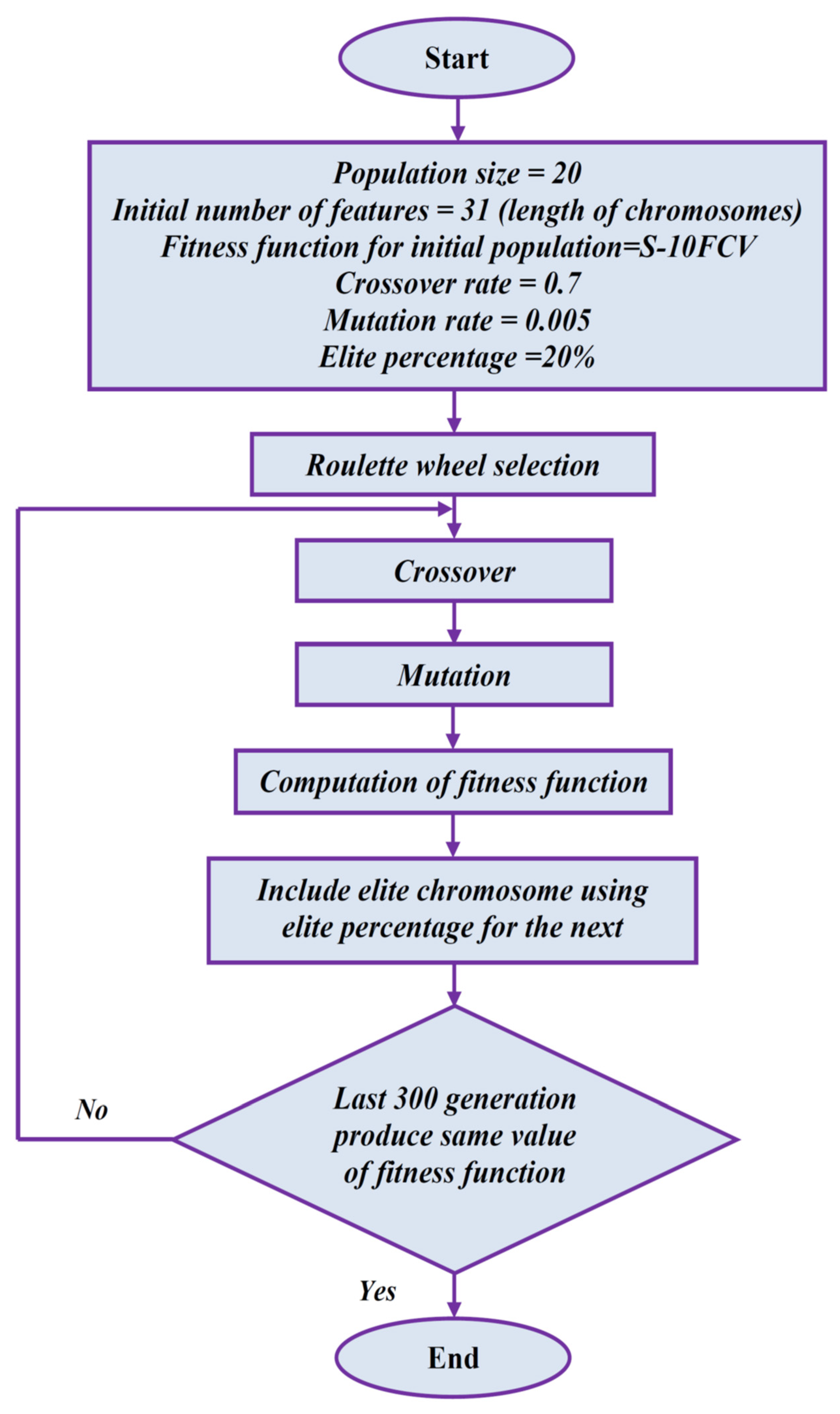
4. Input Feature Selection Using Proposed Algorithm
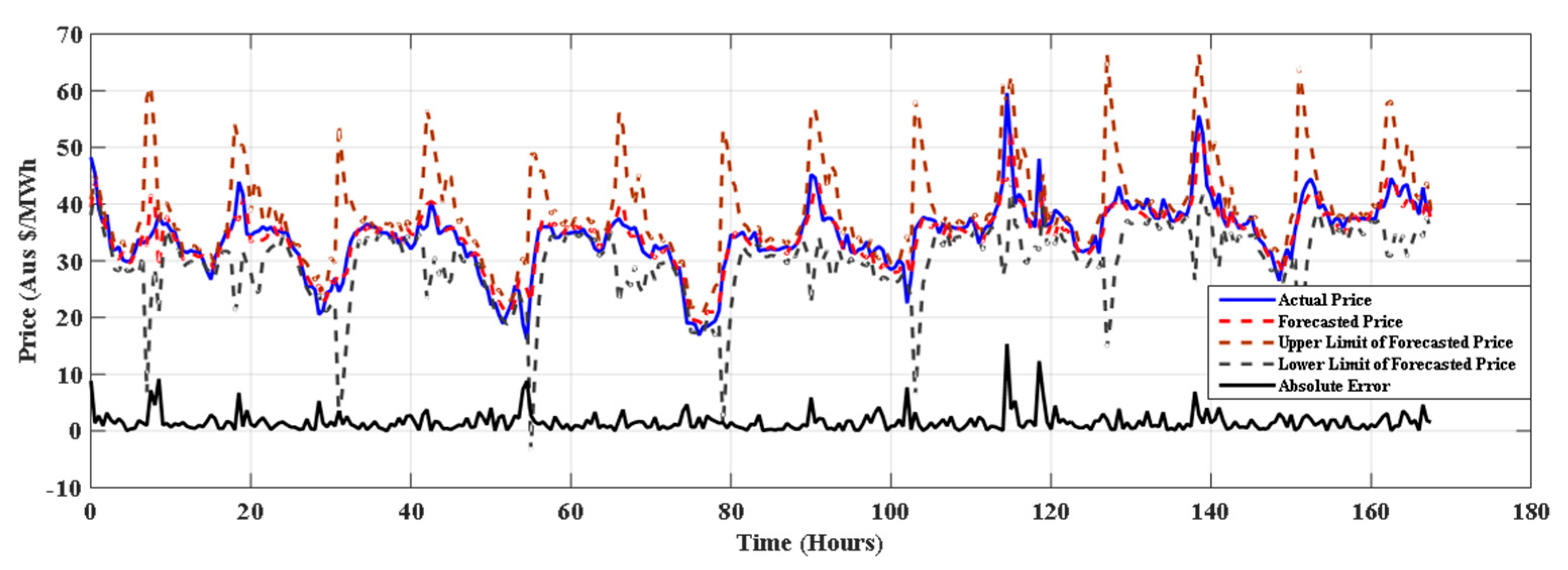
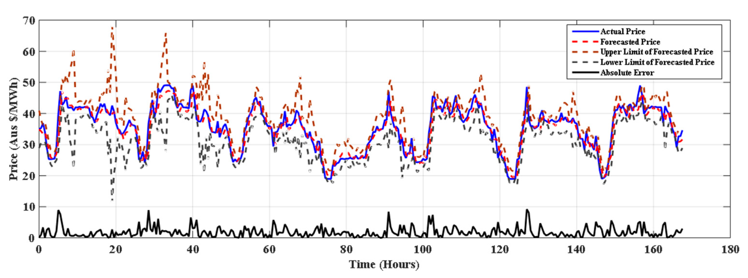
5. Result and Discussion
6. Conclusions
Author Contributions
Funding
Institutional Review Board Statement
Informed Consent Statement
Data Availability Statement
Conflicts of Interest
Abbreviations
| FS | Feature Selection |
| GA | Genetic Algorithm |
| MCP | Market Clearing Prices |
| ANN | Artificial Neural Network |
| SDA | Stacked Denoising Autoencoders |
| FFNN | Feed Forward Neural Networks |
| WT | Wavelet Transform: |
| FA-PSO | Fuzzy Adaptive Particle Swarm Optimization: |
| RF | Random Forest |
| SVM | Support Vector Machine |
| DE | Differential Evolution |
| MI | Mutual Information |
| SMO | Sequential Minimization Optimization |
| QP | Quadratic Programming |
| WoFS | Without Feature Selection |
| KKT | Karush–Kuhan–Tucker |
| 10-FCV | 10-Fold Cross Validation |
| AEMO | Australian Energy Market Operator |
| RMSE | Root-Mean Square Error |
| MAE | Mean Absolute Error |
| MAPE | Mean Absolute Percentage Error |
| EV | Error Variance |
Appendix A
References
- Tso, G.K.; Yau, K.K. Predicting electricity energy consumption: A comparison of regression analysis, decision tree and neural networks. Energy 2007, 32, 1761–1768. [Google Scholar] [CrossRef]
- Alghandoor, A.; Phelan, P.; Villalobos, R.; Phelan, B. US manufacturing aggregate energy intensity decomposition: The application of multivariate regression analysis. Int. J. Energy Res. 2008, 32, 91–106. [Google Scholar] [CrossRef]
- Zaza, F.; Paoletti, C.; LoPresti, R.; Simonetti, E.; Pasquali, M. Multiple regression analysis of hydrogen sulphide poisoning in molten carbonate fuel cells used for waste-to-energy conversions. Int. J. Hydrogen Energy 2011, 36, 8119–8125. [Google Scholar] [CrossRef]
- Kumar, U.; Jain, V. Time series models (Grey-Markov, Grey Model with rolling mechanism and singular spectrum analysis) to forecast energy consumption in India. Energy 2010, 35, 1709–1716. [Google Scholar] [CrossRef]
- Rumbayan, M.; Abudureyimu, A.; Nagasaka, K. Mapping of solar energy potential in Indonesia using artificial neural network and geographical information system. Renew. Sustain. Energy Rev. 2012, 16, 1437–1449. [Google Scholar] [CrossRef]
- Matallanas, E.; Castillo-Cagigal, M.; Gutiérrez, A.; Monasterio-Huelin, F.; Caamano-Martin, E.; Bote, D.M.; Jimenez-Leube, J. Neural network controller for active demand-side management with PV energy in the residential sector. Appl. Energy 2012, 91, 90–97. [Google Scholar] [CrossRef] [Green Version]
- Cheong, C.W. Parametric and non-parametric approaches in evaluating martingale hypothesis of energy spot markets. Math. Comput. Model. 2011, 54, 1499–1509. [Google Scholar] [CrossRef]
- Wesseh, P.K., Jr.; Zoumara, B. Causal independence between energy consumption and economic growth in Liberia: Evidence from a non-parametric bootstrapped causality test. Energy Policy 2012, 50, 518–527. [Google Scholar] [CrossRef]
- Hubicka, K.; Marcjasz, G.; Weron, R. A Note on Averaging Day-Ahead Electricity Price Forecasts across Calibration Windows. IEEE Trans. Sustain. Energy 2019, 10, 321–323. [Google Scholar] [CrossRef]
- Alanis, A.Y. Electricity prices forecasting using artificial neural networks. IEEE Lat. Am. Trans. 2018, 16, 105–111. [Google Scholar] [CrossRef]
- Wang, L.; Zhang, Z.; Chen, J. Short-term electricity price forecasting with stacked denoising autoencoders. IEEE Trans. Power Syst. 2017, 32, 2673–2681. [Google Scholar] [CrossRef]
- Mosbah, H.; El-Hawary, M. Hourly electricity price forecasting for the next month using multilayer neural network. Can. J. Electr. Comput. Eng. 2016, 39, 283–291. [Google Scholar] [CrossRef]
- Sarikprueck, P.; Lee, W.; Kulvanitchaiyanunt, A.; Chen, V.C.P.; Rosenberger, J. Novel Hybrid Market Price Forecasting Method With Data Clustering Techniques for EV Charging Station Application. IEEE Trans. Ind. Appl. 2015, 51, 1987–1996. [Google Scholar] [CrossRef]
- González, J.P.; San Roque, A.M.; Perez, E.A. Forecasting functional time series with a new Hilbertian ARMAX model: Applica-tion to electricity price forecasting. IEEE Trans. Power Syst. 2017, 33, 545–556. [Google Scholar] [CrossRef]
- Anamika; Peesapati, R.; Kumar, N. Electricity Price Forecasting and Classification Through Wavelet–Dynamic Weighted PSO–FFNN Approach. IEEE Syst. J. 2018, 12, 3075–3084. [Google Scholar] [CrossRef]
- Wang, K.; Xu, C.; Zhang, Y.; Guo, S.; Zomaya, A.Y. Robust Big Data Analytics for Electricity Price Forecasting in the Smart Grid. IEEE Trans. Big Data 2019, 5, 34–45. [Google Scholar] [CrossRef]
- Li, P.; Zhang, J.; Li, C.; Zhou, B.; Zhang, Y.; Zhu, M.; Ning, A. Dynamic Similar Sub-Series Selection Method for Time Series Forecasting. IEEE Access 2018, 6, 32532–32542. [Google Scholar] [CrossRef]
- Tahmasebifar, R.; Sheikh-El-Eslami, M.K.; Kheirollahi, R. Point and interval forecasting of real-time and day-ahead electricity prices by a novel hybrid approach. IET Gener. Transm. Distrib. 2017, 11, 2173–2183. [Google Scholar] [CrossRef]
- Abedinia, O.; Amjady, N.; Zareipour, H. A New Feature Selection Technique for Load and Price Forecast of Electrical Power Systems. IEEE Trans. Power Syst. 2017, 32, 62–74. [Google Scholar] [CrossRef]
- González, C.; Mira-McWilliams, J.; Juárez, I. Important variable assessment and electricity price forecasting based on regression tree models: Classification and regression trees, Bagging and Random Forests. IET Gener. Transm. Distrib. 2015, 9, 1120–1128. [Google Scholar] [CrossRef]
- Elattar, E.E.; Elsayed, S.K.; Farrag, T.A. Hybrid Local General Regression Neural Network and Harmony Search Algorithm for Electricity Price Forecasting. IEEE Access 2020, 9, 2044–2054. [Google Scholar] [CrossRef]
- Zhang, C.; Li, R.; Shi, H.; Li, F. Deep learning for day-ahead electricity price forecasting. IET Smart Grid 2020, 3, 462–469. [Google Scholar] [CrossRef]
- Zheng, K.; Wen, B.; Wang, Y.; Chen, Q. Impact of electricity price forecasting errors on bidding: A price-taker’s perspective. IET Gener. Transm. Distrib. 2020, 14, 6259–6266. [Google Scholar] [CrossRef]
- Zhang, D.; Li, Q.; Mugera, A.W.; Ling, L. A hybrid model considering cointegration for interval-valued pork price forecasting in China. J. Forecast. 2020, 39, 1324–1341. [Google Scholar] [CrossRef]
- Furqan, A.M.; Younis, S. Multi-Horizon Electricity Load and Price Forecasting using an Interpretable Multi-Head Self-Attention and EEMD-Based Framework. IEEE Access 2021, 9, 85918–85932. [Google Scholar]
- Huang, C.-J.; Shen, Y.; Chen, Y.-H.; Chen, H.-C. A novel hybrid deep neural network model for short-term electricity price forecasting. Int. J. Energy Res. 2021, 45, 2511–2532. [Google Scholar] [CrossRef]
- Srivastava, A.K.; Singh, D.; Pandey, A.S.; Maini, T. A Novel Feature Selection and Short-Term Price Forecasting Based on a Decision Tree (J48) Model. Energies 2019, 12, 3665. [Google Scholar] [CrossRef] [Green Version]
- Srivastava, A.K.; Singh, D.; Pandey, A.S. Short Term Load Forecasting Using Regression Trees: Ramdom Forest, Bagging & M5P. Int. J. Adv. Trends Comput. Sci. Eng. 2020, 9, 1898. [Google Scholar]


| Name of Variable | Name of Input | Timing of Variable |
|---|---|---|
| Load (Lo) | Lo6 | Lo(D-23:00) |
| Lo5 | Lo(D-23:30) | |
| Lo4 | Lo(D-24:00) | |
| Lo3 | Lo(D-01:30) | |
| Lo2 | Lo(D-01:00) | |
| Lo1 | Lo(D-00.30) | |
| Price (Pr) | Pr6 | Pr(D-23:00) |
| Pr5 | Pr(D-23:30) | |
| Pr4 | Pr(D-24:00) | |
| Pr3 | Pr(D-01:30) | |
| Pr2 | Pr(D-01:00) | |
| Pr1 | Pr(D-00.30) | |
| Wind Speed (Wi) | Wi6 | Wi(D-23:00) |
| Wi5 | Wi(D-23:30) | |
| Wi4 | Wi(D-24:00) | |
| Wi3 | Wi(D-01:30) | |
| Wi2 | Wi(D-01:00) | |
| Wi1 | Wi(D-00.30) | |
| Temperature (Te) | Te6 | Te(D-23:00) |
| Te5 | Te(D-23:30) | |
| Te4 | Te(D-24:00) | |
| Te3 | Te(D-01:30) | |
| Te2 | Te(D-01:00) | |
| Te1 | Te(D-00.30) | |
| Humidity (Hu) | Hu6 | Hu(D-23:00) |
| Hu5 | Hu(D-23:30) | |
| Hu4 | Hu(D-24:00) | |
| Hu3 | Hu(D-01:30) | |
| Hu2 | Hu(D-01:00) | |
| Hu1 | Hu(D-00.30) | |
| Day Timing (Hto) | Hto | Hto(D-00.00) |
| Feature Name | Number of Time Selected | Feature Name | Number of Time Selected |
|---|---|---|---|
| Lo6 | 16 | Wi2 | 20 |
| Lo5 | 10 | Wi1 | 17 |
| Lo4 | 23 | Te6 | 14 |
| Lo3 | 16 | Te5 | 19 |
| Lo2 | 18 | Te4 | 19 |
| Lo1 | 20 | Te3 | 11 |
| Pr6 | 15 | Te2 | 16 |
| Pr5 | 18 | Te1 | 21 |
| Pr4 | 22 | Hu6 | 23 |
| Pr3 | 17 | Hu5 | 20 |
| Pr2 | 18 | Hu4 | 15 |
| Pr1 | 36 | Hu3 | 10 |
| Wi6 | 21 | Hu2 | 18 |
| Wi5 | 13 | Hu1 | 18 |
| Wi4 | 18 | Hto | 24 |
| Wi3 | 15 |
| Feature Name | Winter | Spring | Summer |
|---|---|---|---|
| Lo6 | 8 | 4 | 4 |
| Lo5 | 3 | 4 | 3 |
| Lo4 | 5 | 8 | 10 |
| Lo3 | 4 | 6 | 6 |
| Lo2 | 3 | 7 | 8 |
| Lo1 | 9 | 5 | 6 |
| Pr6 | 3 | 6 | 6 |
| Pr5 | 4 | 8 | 6 |
| Pr4 | 9 | 7 | 6 |
| Pr3 | 7 | 5 | 5 |
| Pr2 | 5 | 7 | 6 |
| Pr1 | 12 | 12 | 12 |
| Wi6 | 7 | 7 | 7 |
| Wi5 | 4 | 5 | 4 |
| Wi4 | 7 | 6 | 5 |
| Wi3 | 6 | 4 | 5 |
| Wi2 | 5 | 7 | 8 |
| Wi1 | 5 | 7 | 5 |
| Te6 | 3 | 7 | 4 |
| Te5 | 6 | 5 | 8 |
| Te4 | 6 | 6 | 7 |
| Te3 | 4 | 2 | 5 |
| Te2 | 6 | 7 | 3 |
| Te1 | 6 | 7 | 8 |
| Hu6 | 6 | 10 | 7 |
| Hu5 | 6 | 7 | 6 |
| Hu4 | 6 | 3 | 6 |
| Hu3 | 4 | 3 | 3 |
| Hu2 | 6 | 5 | 7 |
| Hu1 | 7 | 6 | 5 |
| Hto | 7 | 9 | 8 |
| Sr. No. | Error Measures | Methods | Season | Average | ||
|---|---|---|---|---|---|---|
| Winter (22–28 August 2015) | Spring (22–28 October 2015) | Summer (22–28 January 2016) | ||||
| 1 | Mean Absolute Percentage Error (MAPE) | J48 | 12.45 | 9.30 | 10.42 | 10.72 |
| J48+ FS | 11.40 | 8.41 | 8.86 | 9.56 | ||
| Bagging | 7.86 | 7.67 | 8.61 | 8.05 | ||
| Bagging+ FS | 7.98 | 7.31 | 8.43 | 7.91 | ||
| M5P | 6.40 | 6.12 | 7.68 | 6.73 | ||
| M5P+ FS | 6.05 | 5.77 | 6.47 | 6.10 | ||
| SMO regression | 5.25 | 5.73 | 5.35 | 5.44 | ||
| SMO regression+ FS | 4.85 | 5.26 | 5.28 | 5.13 | ||
| 2 | Mean Absolute Error (MAE) | J48 | 4.09 | 3.34 | 3.88 | 3.77 |
| J48+ FS | 3.74 | 3.07 | 3.29 | 3.37 | ||
| Bagging | 2.62 | 2.76 | 3.24 | 2.87 | ||
| Bagging+ FS | 2.68 | 2.57 | 3.19 | 2.81 | ||
| M5P | 2.14 | 2.19 | 3.65 | 2.66 | ||
| M5P+ FS | 2.03 | 2.07 | 2.74 | 2.28 | ||
| SMO regression | 1.75 | 1.99 | 2.11 | 1.95 | ||
| SMO regression+ FS | 1.60 | 1.82 | 2.07 | 1.83 | ||
| 3 | Root Mean Square Error (RMSE) | J48 | 5.37 | 4.35 | 6.91 | 5.55 |
| J48+ FS | 4.96 | 4.05 | 5.20 | 4.74 | ||
| Bagging | 3.47 | 3.67 | 5.10 | 4.08 | ||
| Bagging+ FS | 3.55 | 3.54 | 5.12 | 4.07 | ||
| M5P | 3.56 | 2.96 | 13.06 | 6.53 | ||
| M5P+ FS | 3.04 | 2.86 | 6.83 | 4.24 | ||
| SMO regression | 2.62 | 2.75 | 4.07 | 3.15 | ||
| SMO regression+ FS | 2.39 | 2.49 | 4.00 | 2.96 | ||
4 | Error Variance (EV) | J48 | 0.0102 | 0.0062 | 0.0271 | 0.0145 |
| J48+ FS | 0.009 | 0.0055 | 0.0134 | 0.0093 | ||
| Bagging | 0.0044 | 0.0046 | 0.0129 | 0.0073 | ||
| Bagging+ FS | 0.0046 | 0.0047 | 0.0133 | 0.0075 | ||
| M5P | 0.0068 | 0.0032 | 0.1307 | 0.0469 | ||
| M5P+ FS | 0.0043 | 0.0031 | 0.0325 | 0.0133 | ||
| SMO regression | 0.0032 | 0.0029 | 0.01 | 0.0054 | ||
| SMO regression+ FS | 0.0027 | 0.0023 | 0.0097 | 0.0049 | ||
| Sr. No. | Method | Average MAPE | Improvement (%) |
| 1. | SMO regression+ FS | 5.13 | - |
| 2. | J48 | 10.72 | 52.16 |
| 3. | J48+ FS | 9.55 | 46.32 |
| 4. | Bagging | 8.086 | 36.27 |
| 5. | Bagging+ FS | 7.86 | 35.15 |
| 6. | M5P | 6.73 | 23.77 |
| 7. | M5P+ FS | 6.09 | 15.90 |
| 8. | SMO regression | 5.44 | 5.75 |
| Sr. No. | Method | Average MAE | Improvement (%) |
| 1. | SMO regression+ FS | 1.83 | - |
| 2. | J48 | 3.76 | 51.33 |
| 3. | J48+ FS | 3.36 | 45.54 |
| 4. | Bagging | 2.87 | 36.24 |
| 5. | Bagging+ FS | 2.81 | 34.89 |
| 6. | M5P | 2.66 | 31.20 |
| 7. | M5P+ FS | 2.28 | 19.74 |
| 8. | SMO regression | 1.95 | 6.15 |
| Sr. No. | Method | Average RMSE | Improvement (%) |
| 1. | SMO regression+ FS | 2.96 | - |
| 2. | M5P | 6.53 | 54.68 |
| 3. | J48 | 5.55 | 46.64 |
| 4. | J48+ FS | 4.74 | 37.51 |
| 5. | M5P+ FS | 4.24 | 30.23 |
| 6. | Bagging | 4.08 | 27.44 |
| 7. | Bagging+ FS | 4.07 | 27.29 |
| 8. | SMO regression | 3.15 | 5.97 |
| Sr. No. | Days | Winter (22–28 August 2015) | Spring (22–28 October 2015) | Summer (22–28 January 2016) | |||
|---|---|---|---|---|---|---|---|
| SMO Reg | SMO Reg+ FS | SMO Reg | SMO Reg+ FS | SMO Reg | SMO Reg+ FS | ||
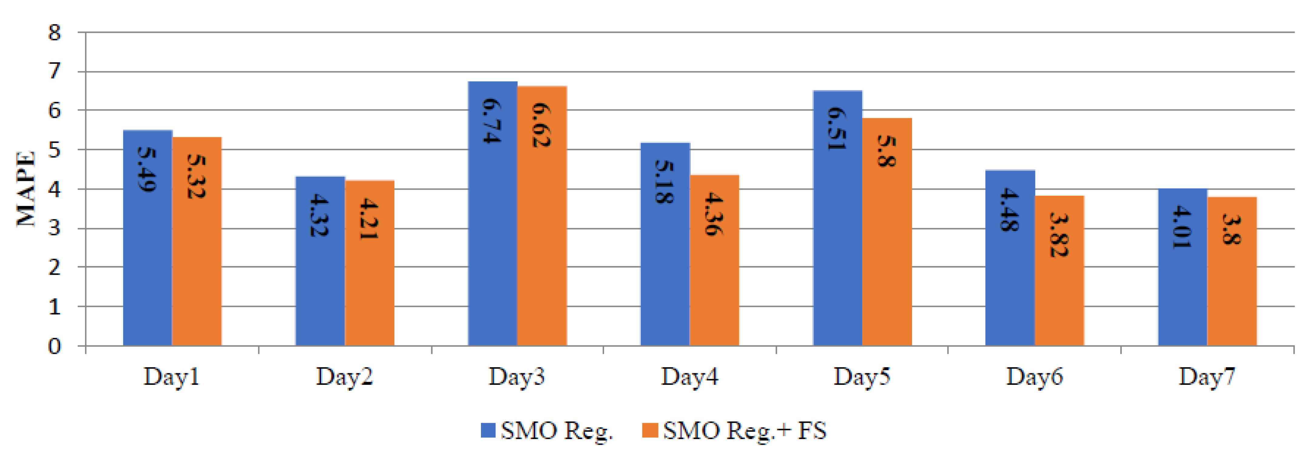
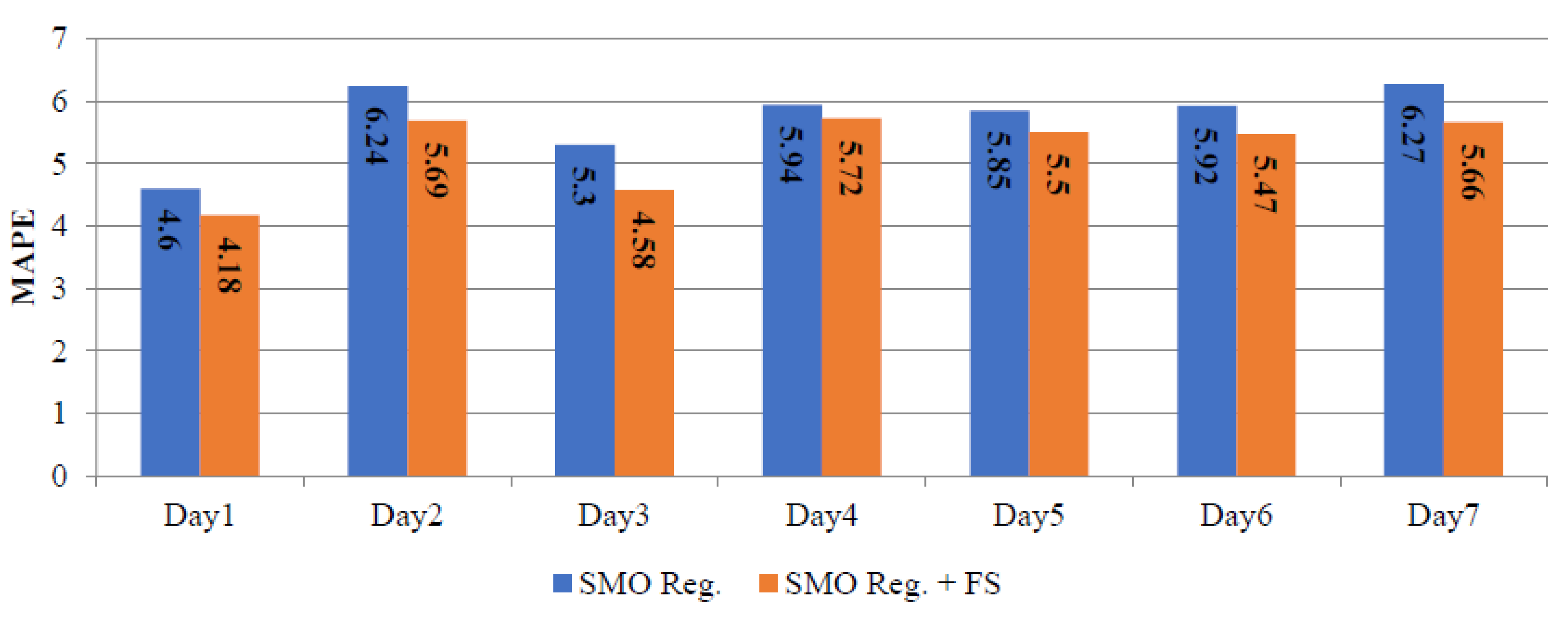
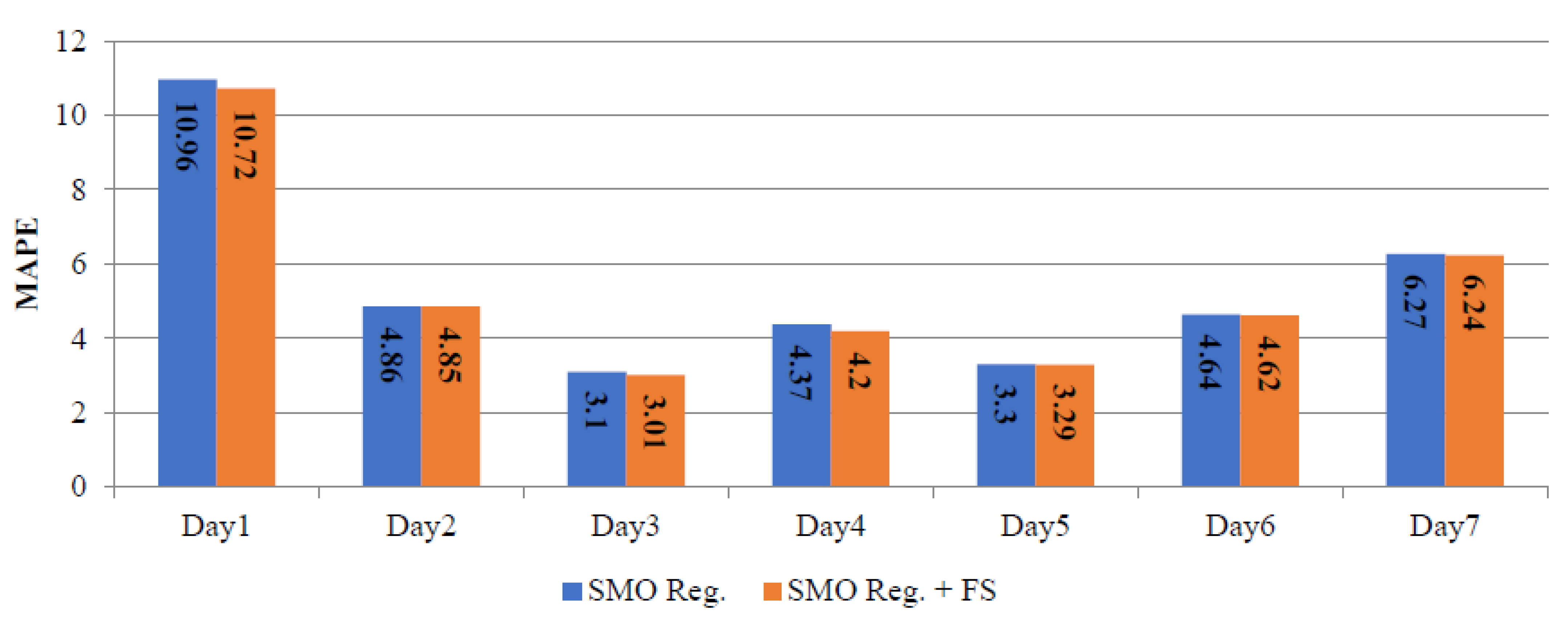
| 1 | Day1 | 5.49 | 5.32 | 4.60 | 4.18 | 10.96 | 10.72 |
| 2 | Day2 | 4.32 | 4.21 | 6.24 | 5.69 | 4.86 | 4.85 |
| 3 | Day3 | 6.74 | 6.62 | 5.30 | 4.58 | 3.1 | 3.01 |
| 4 | Day4 | 5.18 | 4.36 | 5.94 | 5.72 | 4.37 | 4.20 |
| 5 | Day5 | 6.51 | 5.80 | 5.85 | 5.50 | 3.3 | 3.29 |
| 6 | Day6 | 4.48 | 3.82 | 5.92 | 5.47 | 4.64 | 4.62 |
| 7 | Day7 | 4.01 | 3.80 | 6.27 | 5.66 | 6.27 | 6.24 |
| Average | 5.25 | 4.85 | 5.73 | 5.26 | 5.35 | 5.28 | |
Publisher’s Note: MDPI stays neutral with regard to jurisdictional claims in published maps and institutional affiliations. |
© 2021 by the authors. Licensee MDPI, Basel, Switzerland. This article is an open access article distributed under the terms and conditions of the Creative Commons Attribution (CC BY) license (https://creativecommons.org/licenses/by/4.0/).
Share and Cite
Srivastava, A.K.; Pandey, A.S.; Elavarasan, R.M.; Subramaniam, U.; Mekhilef, S.; Mihet-Popa, L. A Novel Hybrid Feature Selection Method for Day-Ahead Electricity Price Forecasting. Energies 2021, 14, 8455. https://0-doi-org.brum.beds.ac.uk/10.3390/en14248455
Srivastava AK, Pandey AS, Elavarasan RM, Subramaniam U, Mekhilef S, Mihet-Popa L. A Novel Hybrid Feature Selection Method for Day-Ahead Electricity Price Forecasting. Energies. 2021; 14(24):8455. https://0-doi-org.brum.beds.ac.uk/10.3390/en14248455
Chicago/Turabian StyleSrivastava, Ankit Kumar, Ajay Shekhar Pandey, Rajvikram Madurai Elavarasan, Umashankar Subramaniam, Saad Mekhilef, and Lucian Mihet-Popa. 2021. "A Novel Hybrid Feature Selection Method for Day-Ahead Electricity Price Forecasting" Energies 14, no. 24: 8455. https://0-doi-org.brum.beds.ac.uk/10.3390/en14248455