Self-Inductance Calculation of the Archimedean Spiral Coil

Abstract

In this paper, a new method to calculate the self-inductance of the Archimedean spiral coil is presented. The proposed method is derived by solving Neumann’s integral formula, and the numerical tool is used to calculate the inductance value. The calculation results are verified with several conventional formulas derived from the Wheeler formula or its modified form and 3D finite element analyses. The comparison with simulation results shows that the conventional formula has an error of above 40% compared to the proposed method, which has below 7% when the wire diameter is reduced. To further check the validity, different sizes of the spiral coil are fabricated by changing the geometrical parameters such as the number of turns, turn spacing, inner radius, outer radius, and wire diameter. Litz wire is chosen for making the spiral coil, and bobbins are made using a 3D printer. Finally, the calculation results are compared with the experimental result. The error between them is less than 2%. The comparison with the conventional formulas, simulation, and measurement results shows the accuracy of the proposed method. This method can be used to calculate the self-inductance of wireless power coils, inductors and antenna design.

1. Introduction

The spiral coil has been widely used in electromagnetic applications such as wireless power transfer, radio frequency identification, near field communication, and biomedical implant. There are many types of spiral coil such as the circular, rectangular, hexagonal, and octagonal spirals [1,2,3,4,5,6,7,8]. In this paper, the Archimedean spiral coil is chosen due to its simple geometry and high performance.

The Archimedean spiral is a circular spiral named after the mathematician Archimedes [9]. It is the locus of points corresponding to the locations over time of a point moving away from a fixed point with a constant speed along a line that rotates with an angular velocity.

To design the spiral coil, one of the main factors is self-inductance. It depends on geometrical parameters such as the number of turns, inner radius, turn spacing, wire diameter, and outer radius. In high-frequency application, the wire diameter is considered an important parameter.

To calculate the self-inductance of spiral coils, many studies have been conducted [10,11,12,13,14,15,16]. However, most of them adopted the Wheeler formula or its modified form, which is an empirical method and does not reflect the real physical phenomena. Moreover, the accuracy of the conventional formulas is limited, and the error increases when the wire diameter is changed. Further, all the parameters which influence the inductance are not included.

In [11], the self-inductance of the circular spiral coil is derived from the modified Wheeler’s formula. This formula is inaccurate for most structures when the wire diameter is just changed. In other words, this formula has not taken into account the wire diameter. The difference between the calculation result and 3D finite element method (FEM) is over 40%.

In [12], the self-inductance of the spiral coil is calculated using the Harold A. Wheeler approximation. It is applied at low frequency applications using an enameled copper wire. Therefore, it is not suitable for high frequency applications using Litz wire.

In [13,14], the self-inductance of a circular-spiral coil is approximated through modification of Wheeler formula. This formula is derived by using the average of the initial and final diameter of a spiral coil and taking their logarithm. The wire diameter has not been taken into account too in these formulas.

In [15], the effect on structural parameters of the spiral coil is studied on the self-inductance. The spiral coils are designed and developed in the FEM-based commercial software and verified experimentally. However, due to the absence of the analytical background, it is highly dependent on the simulation result.

In [16,17], the wire diameter is included in the calculation of the self-inductance. For Litz wire with a uniform wire diameter and an evenly distributed current density, a geometric mean distance method is proposed. In this method, the difference between the calculation result and the FE analysis increase as the number of turns increases.

Instead of the analytical method, the self-inductance of the spiral coil is approximated empirically [18,19,20] simplified the spiral into several concentric circular coils to estimate the self-inductance. This method increases the computational complexity. Therefore, there is some inconsistency between the approximated and measurement value.

The FEM is one of the best methods to calculate the self-inductance of the spiral coil with any geometry. However, it requires computational burden. To address this problem, we propose a new accurate method for the self-inductance of the Archimedean spiral coil. The proposed method is derived analytically by solving Neumann’s integral formula. The Archimedean general equation is used to decide the inner and outer radius of the spiral coil. Each derivation step is presented in detail. The spiral inductance of any configuration can be obtained by putting its parameter numerically in the final inductance equation.

The inductance of several spiral coils are calculated. The calculation results are verified by finite element method (FEM) ANSYS Maxwell software. For experimental validation, a 3D printer is used to construct special bobbins for winding the spiral coil. Finally, a comparison between the calculation and measurement results certify its correctness.

2. The Self-Inductance of the Archimedean Spiral Coil

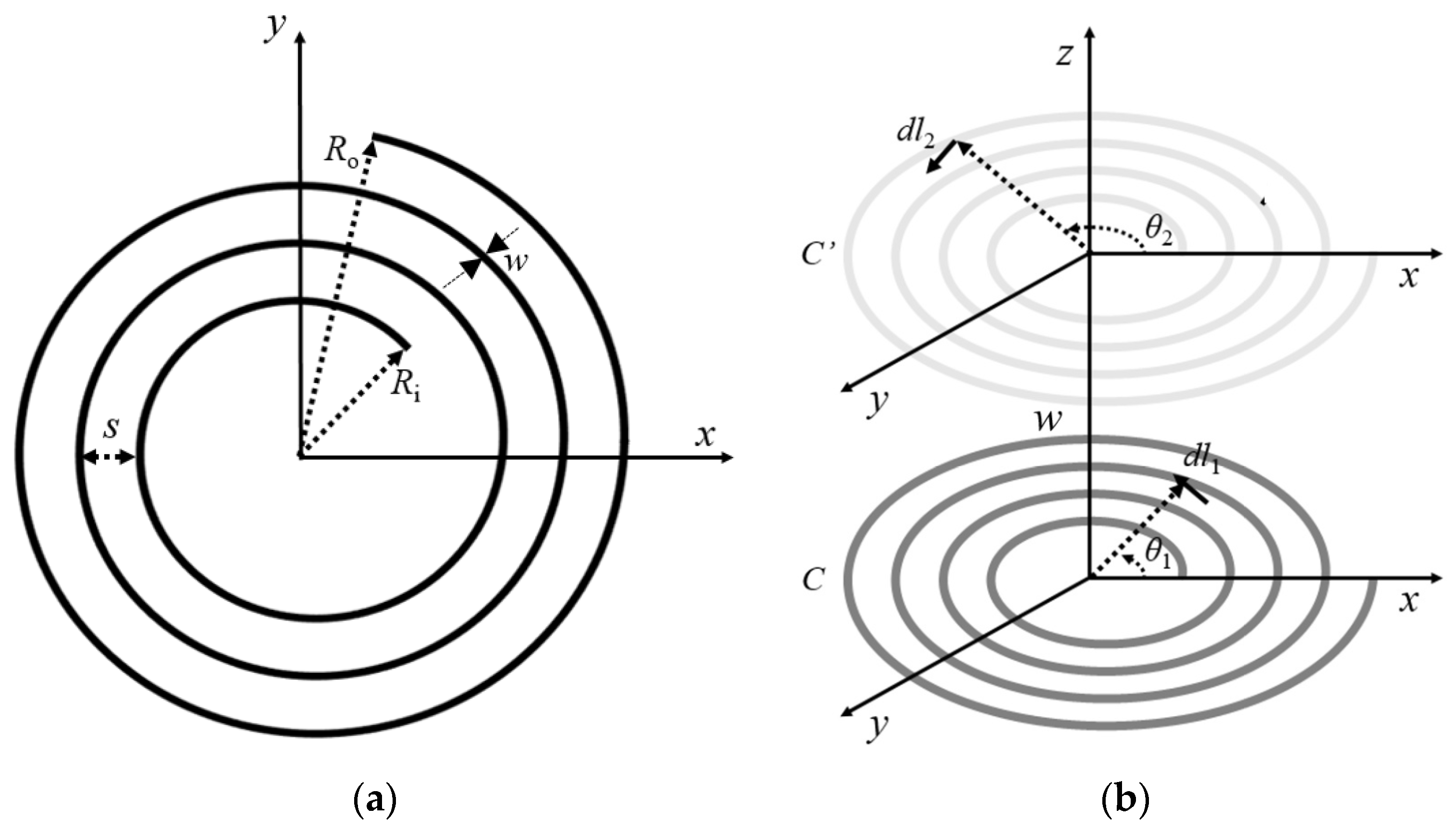
The self-inductance primarily depends on geometric parameters such as the number of turns, the gap between turns, the wire diameter, and the initial and final radius of the Archimedean spiral coil. Figure 1a shows the Archimedean spiral coil. In this paper, the self-inductance of the Archimedean spiral coil can be computed by Neumann’s formula as shown in Equation (1).

Neumann derived this formula for mutual inductance, but it can be used to find self-inductance [21].

$$L=\frac{{\mu }_0}{4\pi }{\displaystyle \underset{C_1}{\oint }{\displaystyle \underset{C_2}{\oint }\frac{d{l}_{1}d{l}_2}{R}}},$$

(1)

where μ₀ is the vacuum permeability, dl₁ and dl₂ are line elements, and R is the distance between dl₁ and dl₂. Eventually, the self-inductance of the Archimedean spiral coil can be determined by finding dl₁, dl₂ and R in Equation (1).

The Archimedean spiral coil can be described by

$$R=R_i+a\theta ,\hspace{1em}{\theta }_i\le \theta \le {\theta }_0,$$

(2)

$$\theta =2\pi N,$$

(3)

$$a=\frac{s+w}{2\pi },$$

(4)

where R_i is an initial radius, s is the gap between turns, a is the pitch factor, θ_i and θ_o are the initial and final angles of the Archimedean spiral coil, N is the number of turns, and w is the wire diameter. The pitch factor a affects the gap between turns. We assume that the spiral coil is placed on the x–y plane.

In Figure 1b, C is the Archimedean spiral coil and it has been moved by the distance of wire diameter w in the z-axis direction to get its duplicate C′. The duplicate coil C’ is exactly same and coaxial with the original coil, C. Now, C′ can be used as a secondary spiral coil. The self-inductance is due to the flux produced by the current in spiral C that links the C′. Thus, the self-inductance of the spiral coil C can be calculated by finding the mutual inductance between the original coil C and its duplicate coil C′.

In Figure 1b, line elements dl₁ and dl₂ are represented as follows:

$$d{l}_1=R_{1}d{\theta }_1,$$

(5)

$$R_1=R_i+a{\theta }_1,$$

(6)

$$d{l}_2=R_{2}d{\theta }_2,$$

(7)

$$R_2=R_i+a{\theta }_2,$$

(8)

The dot product of Equations (5) and (7) is shown in Equation (9)

$$d{l}_1·d{l}_2=\left(R_i+a{\theta }_1\right)\left(R_i+a{\theta }_2\right)\cos \left({\theta }_2-{\theta }_1\right)d{\theta }_{1}d{\theta }_2,$$

(9)

The distance R between R₁ and R₂ can be denoted using the law of cosines

$$\begin{array}{l}{R}^2={\left(R_i+a{\theta }_1\right)}^2+{\left(R_i+a{\theta }_2\right)}^2\\ -2\left(R_i+a{\theta }_1\right)\left(R_i+a{\theta }_2\right)\cos \left({\theta }_2-{\theta }_1\right)+w^2,\end{array}$$

(10)

Substituting Equations (9) and (10) in Equation (1), the self-inductance of Archimedean spiral coil is obtained in Equation (11)

$$\begin{array}{l}L=\frac{{\mu }_0}{4\pi }{\displaystyle \underset{2\pi N}{\iint }\frac{kd{\theta }_{1}d{\theta }_2}{\sqrt{{\left(R_i+a{\theta }_1\right)}^2+{\left(R_i+a{\theta }_2\right)}^2-2k+w^2}},}\\ \\ \hfill k=\left(R_i+a{\theta }_1\right)\left(R_i+a{\theta }_2\right)\cos \left({\theta }_2-{\theta }_1\right)\hfill \end{array}$$

(11)

Since Equation (11) is a double integral form, it cannot be represented by an elementary formula, and thus it is solved by a numerical tool. This is a disadvantage for the proposed method. However, maintaining the accuracy in various spiral coils is its powerful advantage.

3. Comparison Results

In order to compare the result of the proposed method with the FEM and conventional formulas results, the maximum size of the spiral coil is constrained to the maximum capability of the printer. Hence, the outer diameter of our big coil size is fixed to 170 mm. By considering this limitation, the inductance is calculated for several coils with a different number of turns, the gap between turns and wire diameter, inner radius, outer radius.

Regarding FEM simulation, it is performed in ANSYS Maxwell 15. The solution type is chosen as Magneto static, and mesh is assigned as length based. The maximum length of the element is selected as default value. For the purpose of simplicity, constant current is distributed at the cross section of the coil.

In [11], the modified Wheeler’s formula for a single-layer spiral coil is given by Equation (12)

$$L=\frac{N^2{\left(D_o-N\left(w+s\right)\right)}^2}{16D_o+28N\left(w+s\right)}\times \frac{39.37}{{10}^6},$$

(12)

where Do is the outer diameter of the spiral coil. Equation (12) shows that self-inductance will increase when the number of turns, outer diameter, the gap between turns, and wire diameter increase.

In the next case, the Equation (13) is considered, which was another modified Wheeler’s formula, similarly to Equation (12).

$$\begin{array}{l}L\left(\mu \mathrm{H}\right)=\frac{r^2{A}^2}{(30A-11D_i)},\\ A=\frac{\left(D_i+N\left(w+s\right)\right)}{2}\end{array}$$

(13)

where Di is the inner diameter, s is the gap between turns, w is the wire diameter, N is the number of turns. The unit of D_i, s and w is in inches. Equation (13) includes the inner diameter while Equation (12) has the outer diameter.

To further show the validity of the proposed method, it is compared to other self-inductance formulas. In Equation (14), the self-inductance is evaluated using the concepts of geometric mean distance, arithmetic mean distance, and arithmetic mean square distance [13]. The resulting expression is shown below.

$$\begin{array}{l}L=\frac{{\mu }_o{N}^2(\frac{d_{out}+d_{in}}{2})}{2}\left[\ln \left(\frac{2.46}{(\frac{d_{out}-d_{in}}{d_{out}+d_{in}})}\right)+0.2{\gamma }^2\right],\\ \hfill \gamma =\frac{\left(d_{out}-d_{in}\right)}{\left(d_{out}+d_{in}\right)}\hfill \end{array}$$

(14)

where d_in and d_out are the inner and outer diameter of the spiral coil, and γ is the fill ratio.

Equation (15) expresses the simplified inductance of the single-layer circular coil [14].

$$\begin{array}{l}L=\frac{{\mu }_o{N}^2{d}_{avg}{C}_1}{2}\left(\left(\ln \frac{C_2}{\sigma }\right)+C_3\gamma +C_4{\gamma }^2\right),\\ \hfill d_{avg}=\frac{d_{out}+d_{in}}{2}\hfill \end{array}$$

(15)

where d_avg is the mean diameter, and C is the layout dependent coefficient. For the circular coil, C₁ is1.0, C₂ is 2.45, C₃ is 0 and C₄ is 0.2.

Another self-inductance expression based on the geometric mean distance principle for a spiral coil is derived [16].

$$\begin{array}{l}L=\frac{{\mu }_o}{4\pi }{\displaystyle \underset{0}{\overset{\theta }{\int }}{\displaystyle \underset{0}{\overset{\theta }{\int }}\frac{1}{\sqrt{{\left(X_2-x_1\right)}^2+{\left(Y_2-y_1\right)}^2+{\left(g\right)}^2}}}}\\ \hfill \left[\left(a\cos {\theta }_1-y_1\right)\left(a\cos {\theta }_2-Y_2\right)\right.\hfill \\ \hfill \left.+\left(a\sin {\theta }_1+x_1\right)\left(a\sin {\theta }_2+X_2\right)\right]d{\theta }_{1}d{\theta }_2,\end{array}$$

(16)

where a = γ/(2π), θ = 2Nπ, x₁ = (R_i + aθ₁)cosθ₁, y₁ = (R_i + aθ₁)sinθ₁, X₂ = (R_i + aθ₂) cosθ₂, Y₂ = (R_i + aθ₂)sinθ₂, R_i is the inner radius, and g is the geometric mean distance of the cross section of the wire

$$g=\frac{e^{-\frac{1}{4}}w}{2}=0.3894w,$$

(17)

where w is the wire diameter. Equations (12)–(16) are well-known self-inductance formulas. Their results are presented in the following Tables.

3.1. Case 1

In

Table 1. Comparison results.

Parameters			Results
N	s (mm)	w (mm)	FEM (µH)	(11) (µH)	Error (%)	(12) (µH)	Error (%)	(13) (µH)	Error (%)
5	11.40	3.6	1.92	1.85	3.6	1.84	4.16	1.84	4.16
6	8.90	3.6	2.71	2.63	2.9	2.65	2.21	2.65	2.21
7	7.11	3.6	3.60	3.58	0.5	3.61	−0.27	3.61	−0.27
8	5.77	3.6	4.70	4.69	0.2	4.71	−0.21	4.71	−0.21
9	4.33	3.6	6.01	5.99	0.3	5.97	0.66	5.97	0.66
10	3.90	3.6	7.50	7.56	−0.8	7.37	1.73	7.37	1.73
11	3.21	3.6	9.14	9.09	0.54	8.96	1.96	8.91	2.51
12	2.65	3.6	10.55	10.50	0.47	10.61	−0.56	10.61	−0.56
13	2.16	3.6	12.34	12.28	0.48	12.98	−5.18	12.44	−0.81
14	1.75	3.6	14.49	14.46	0.20	14.48	0.06	14.43	0.41
15	1.40	3.6	16.47	16.38	0.54	16.58	−0.66	16.58	−0.66

, the inductances of different coil geometries are computed for constant wire diameter w, while in

Table 2. Comparison Results with changing wire diameters.

Parameters			Results
N	s (mm)	w (mm)	FEM (µH)	(11) (µH)	Error (%)	(12) (µH)	Error (%)
5	14	1	3.17	2.97	6.30	1.84	41.95
5	13	2	2.34	2.21	5.55	1.84	21.36
5	11.40	3.6	1.92	1.85	3.6	1.84	4.16
7	9.71	1	6.07	5.75	5.27	3.61	40.52
7	8.71	2	4.50	4.27	5.11	3.61	19.77
7	7.11	3.6	3.60	3.58	0.5	3.61	−0.27
10	6.50	1	12.92	12.07	6.57	7.37	42.95
10	5.50	2	9.51	9.03	5.04	7.37	22.50
10	3.90	3.6	7.50	7.56	−0.8	7.37	1.73
12	5.25	1	17.84	16.89	5.32	10.61	40.52
12	4.25	2	13.15	12.55	4.56	10.61	19.31
12	2.65	3.6	10.55	10.50	0.47	10.61	−0.56
14	4.35	1	24.18	23.18	6.07	14.48	41.32
14	3.35	2	18.16	17.27	4.90	14.48	20.26
14	1.75	3.6	14.49	14.46	0.20	14.48	0.06

, it is calculated when w is changed. The error of inductance of the proposed method, Equation (11), and other conventional formulas, Equations (12) and (13), are compared relative to FEM.

In Table 1, the simulation results using FEM are compared with the three different methods. Equation (11) is the proposed formula, Equation (12) is the modified Wheeler’s formula and Equation (13) is another modified Wheeler formula. It is deduced from the above comparison Tables that when the number of turns is increased, the error is generally decreased. For a larger number of turns, all cases have a similar difference. Therefore, the number of turns was limited to 15 turns. Table 1 shows the comparison results for when the wire diameter is fixed. Equations (11)–(13) have similar errors compared to FEM.

The wire diameter affects the self-inductance. Therefore, it is necessary to compare the self-inductance of the spiral for the changing wire diameter. Table 2 indicates that the error of the inductance values of the conventional formulas increases sharply when the wire diameter decreases. However, the accuracy of the conventional formula improves with the increase in wire diameter. On the other hand, the proposed method maintains reasonable accuracy for all cases. For a very small diameter wire, Maxwell 15 was unable to solve inductance. Therefore, we assume that the current approximation of the proposed method is good until 1 mm wire diameter.

In both, Equations (12) and (13), the error increases as the wire diameter decreases. However, the comparison Table of Equation (13) for changing w is not included due to avoidance of repetition.

The influence of wire diameter on the inductance of the coil can be explained by the high-frequency model of AC resistance. It states that when the wire diameter decreases, the AC resistance of the wire also decreases. The decrease in AC resistance will strengthen the magnetic field. The high magnetic field increases the flux linkage, and thus the inductance [22].

3.2. Case 2

Table 3. Comparison results with different conventional self-inductance formulas.

Parameters			Results
N	s (mm)	w (mm)	FEM (µH)	(11) (µH)	(14) (µH)	(15) (µH)	(16) (µH)
5	11.40	3.6	1.92	1.85	1.88	1.88	2.54
6	8.90	3.6	2.71	2.63	2.71	2.70	3.62
7	7.11	3.6	3.60	3.58	3.69	3.68	4.92
8	5.77	3.6	4.70	4.69	4.82	4.80	6.44
9	4.33	3.6	6.01	5.99	6.09	6.08	8.20
10	3.90	3.6	7.50	7.56	7.52	7.50	10.34
11	3.21	3.6	9.14	9.09	9.10	9.07	12.44
12	2.65	3.6	10.55	10.50	10.84	10.80	14.42
13	2.16	3.6	12.34	12.28	12.72	12.68	16.86
14	1.75	3.6	14.49	14.46	14.75	14.70	19.81
15	1.40	3.6	16.47	16.38	16.93	16.88	22.50

shows the comparison of the inductance of the proposed method with three different conventional formulas for the calculation of self-inductance of the spiral coil. Their errors are represented in

Table 4. Comparison results of Errors.

Parameters			Errors
N	s (mm)	w (mm)	(11) (%)	(14) (%)	(15) (%)	(16) (%)
5	11.40	3.6	3.6	2.08	2.08	−32.29
6	8.90	3.6	2.9	0	0.36	−33.57
7	7.11	3.6	0.5	−2.50	−2.22	−36.67
8	5.77	3.6	0.2	−2.55	−2.12	−37.02
9	4.33	3.6	0.3	−1.33	−1.16	−36.43
10	3.90	3.6	−0.8	−0.26	0	−37.60
11	3.21	3.6	0.54	0.43	0.76	−36.10
12	2.65	3.6	0.47	−2.74	−2.36	−36.68
13	2.16	3.6	0.48	−3.07	−2.75	−36.62
14	1.75	3.6	0.20	−1.79	−1.44	−36.71
15	1.40	3.6	0.54	−2.79	−2.48	−36.61

In Table 4, Equations (14) and (15) show relatively low errors and Equation (16) indicates relatively high errors for all cases. In Equations (14) and (15), wire diameter, which is one of the important parameters to determine self-inductance, is not considered. If the wire diameter is changed from a higher to a lower value, the results will be similar to the other conventional formulas, which is shown in Table 2.

Although Equation (16) applied a geometric mean distance in order to consider the wire diameter, it shows large errors compared to the FEM and other conventional formulas. In Equations (12)–(15), the errors decrease when the number of turns was increased. However, Equation (16) showed consistently large errors even if the number of turns was changed. However, the proposed method maintains an error below 7% for all cases. These results show the validity of the proposed method.

4. Experiment Process

4.1. Bobbin

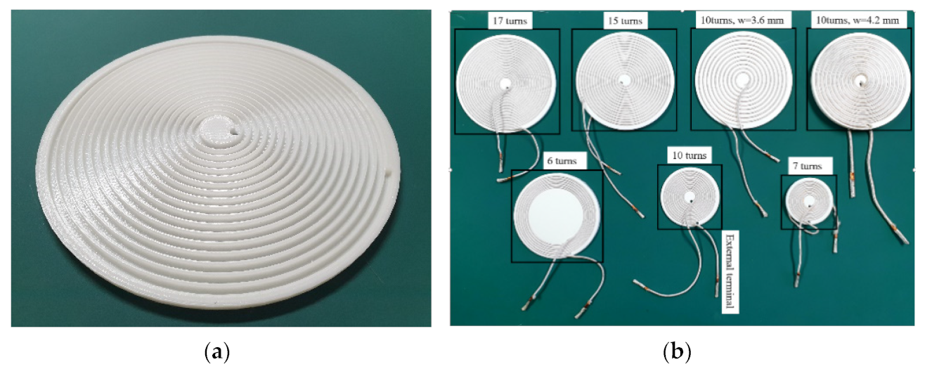
To validate the proposed method for the self-inductance of the spiral coil, seven different sizes of spiral coils are constructed for the experimental purpose. These are selected from the combination of the number of turns, inner radius, wire diameter, outer radius and the gap between turns. In order to hold the wire position in the spiral coil, a special bobbin is designed and printed using a 3D printer.

Two different sizes of Litz wire are selected for making the spiral coil. To make the bobbin, the total diameter of the Litz wire should be decided. The total diameter of the Litz wire is 3.6 mm and 4.2 mm. It is empirically decided by

$$D_e=1.6\left(\sqrt{{\left(\raisebox{1ex}{$D_s$}\!\left/ \!\raisebox{-1ex}{$2$}\right.\right)}^2{N}_s}\right)2,$$

(18)

where D_e is an estimated diameter of the Litz wire, D_s is the diameter of one strand of wire and N_s is the total number of strands. Due to the printing size of the 3D printer, the bobbin size is limited to 170 mm. The polylactic acid filament is used. Figure 2 shows spiral coils with the bobbin.

4.2. Selection of Wire

For the selection of the wire, the operating frequency and current are key components. The operating frequency not only influences the wire construction but is also used to determine the wire gauge. The eddy current loss occurs due to the high frequency effect. The eddy current loss increases with the operating frequency. The source of this loss is the skin effect and proximity effect, which can be reduced by using the Litz wire. Therefore, the Litz was chosen for the spiral coil [23].

The Litz wire has formed by combining many strands of thin insulated wire together side by side. It is used to carry the high frequency current as each insulated strands carry a part of the current and reduce the skin and proximity effect [24].

In this paper, the Litz wire with 500 strands and 0.12 mm diameter are used considering the operating frequency and current. The applied frequency is 10 kHz.

4.3. Total Length of Litz Wire

In order to calculate the resistance, it is necessary to accurately estimate the total length of the spiral coil. The total length is calculated by

$$\begin{array}{l}{L}_{tot}={\displaystyle \underset{{\theta }_i}{\overset{{\theta }_o}{\int }}\sqrt{R_o^2+{\left(\frac{d{R}_0}{d\theta }\right)}^{2}d\theta }}+extra length,\\ \\ \hfill R_o=R_i+a\theta \hfill \end{array}$$

(19)

In Figure 2b, an extra length can be added to the end of the spiral coil for measurement or connection purpose.

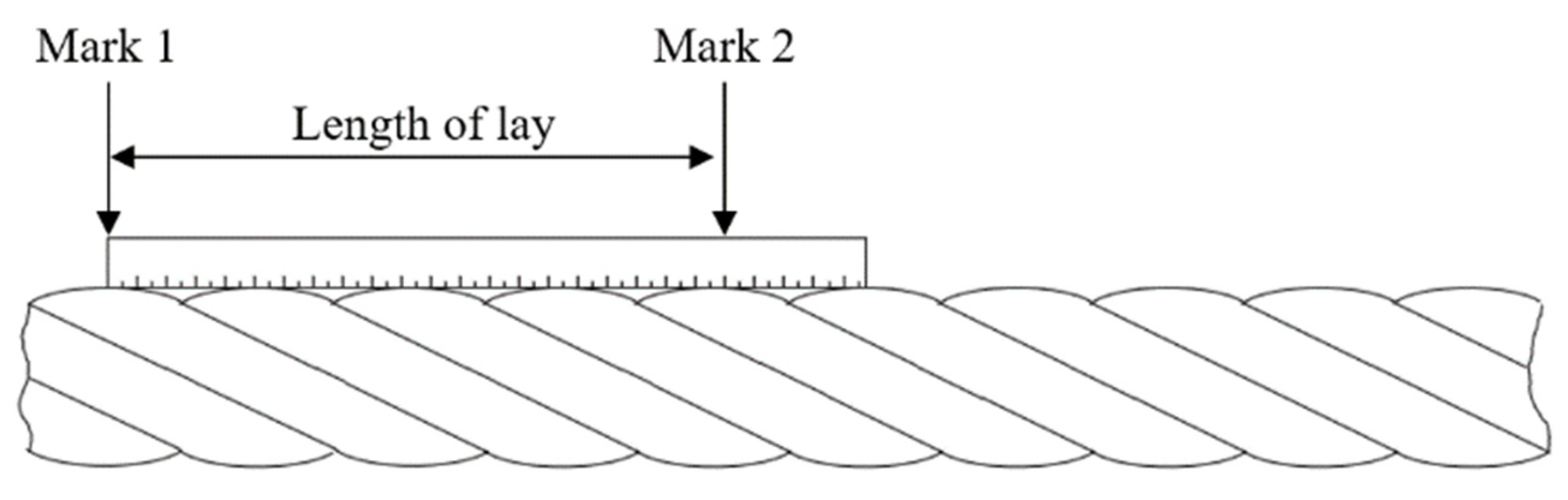
Because the Litz wire consists of many thin wire strands, individually insulated and twisted or woven together, the effective length of the spiral coil is longer than the calculated one in Equation (19). To perform the measurement, a strand is selected and marked on the surface, as shown in Figure 3. The next strand on the same side of the surface is also marked. Then, the distance between the marks is measured.

To increase accuracy, the measurement is taken over several lengths of lay. This method has disadvantages, for example, it takes a lot of time and must be repeated a large number of times to find the accurate value of the length of lay.

$$L_{eff}=L_{tot}{k}_{twist},$$

(20)

In Equation (20), twist effect k_twist depends on the lengths of lay and the twist pattern. The k_twist range of the Litz wire under 5000 strand is from 1.03 to 1.05.

Table 5. Comparison between the calculated and the measured length.

Number of Turns	Calculated Length (m)	Measured Length (m)	Difference (%)
6 (large Ri)	2.63	2.94	10.54
7	1.34	1.43	6.29
10 (small Ro)	2.19	2.35	6.80
10 (w = 4.2)	2.98	3.10	3.80
10	2.98	3.15	5.39
15	4.47	5	10.6
17	5.07	5.58	9.13

shows the comparison result between the calculated and the measures length of the spiral coil.

4.4. Calculation of the DC Resistance of a Coil

The length of the spiral coil also affects the resistance. Therefore, it is important to compute it accurately. It can be calculated by Equation (21).

$$R=\frac{l(mm)}{\sigma n\pi r^2},$$

(21)

where l the length of wire in millimeter is, σ is constant and its values is 58,000, n is the number of strands and r is the radius of a single strand.

The DC resistances of the above spiral coils are calculated and also verified by measurement with a Gwinstek LCR-6200. The comparison result and their differences are shown in

Table 6. Comparison between the calculated and the measured DC resistance of coil.

Number of Turns	Calculated DCR (mΩ)	Measured DCR (mΩ)	Difference (%)
6 (large Ri)	11.54	11.29	0.68
7	5.88	6.29	6.51
10 (small Ro)	9.61	9.94	3.42
10 (w = 4.2)	5.67	5.83	2.74
10	13.08	14.98	12.08
15	21.95	22.93	4.27
17	24.49	25.69	4.67

.

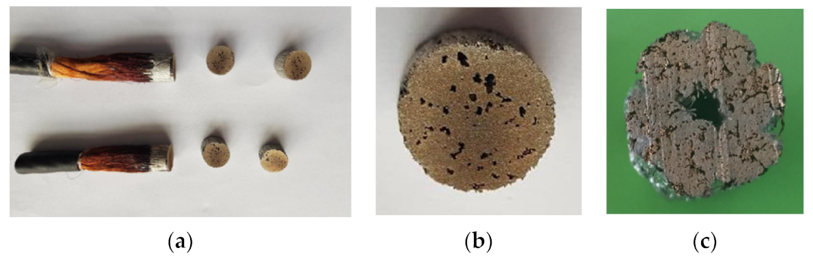
4.5. Soldering Quality

Several factors can be affected when calculating resistance and self-inductance. A soldering quality is one of them. From previous results, the wire diameter was an important factor for the self-inductance. Because actual wire diameter can be reduced due to the soldering, a sequential soldering process is required.

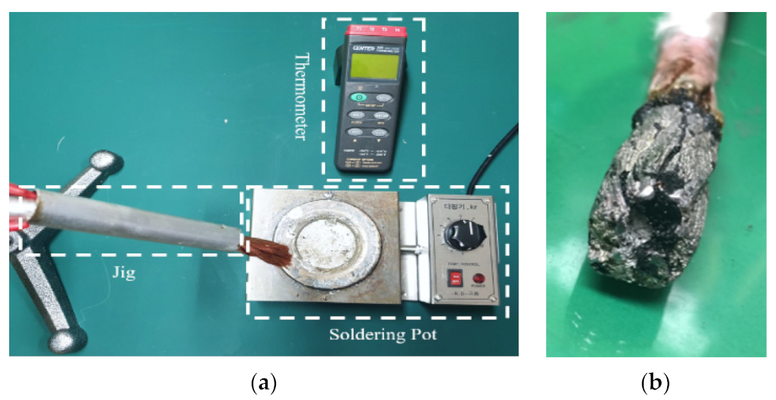
In some cases, the solder pot and solder temperature must be compatible. The soldering temperature varies with the type and the number of the strand of Litz wire being soldered. Therefore, an appropriate solder set and special jig should be prepared as shown in Figure 4a.

The high temperatures are used to remove the enamel from each insulated strand. However, too high a temperature will burn off not only the enamel but also the strands and it will leave a black dreg, as shown in Figure 4b. Inspection of a crosscut of the soldered end can be achieved to ensure a good solder termination, as indicated in Figure 5a.

With a properly soldered joint, strands will be visible with solder tightly surrounding them as shown in Figure 5b. However, in a poorly soldered joint, as shown in Figure 5c, the strands are still with the visible insulator, increasing the resistance. In that case, solder temperature or immersion time will need to be increased. The number of strands and the wire diameter should be considered when the solder pot and solder temperature are decided, empirically.

5. Experimental Results

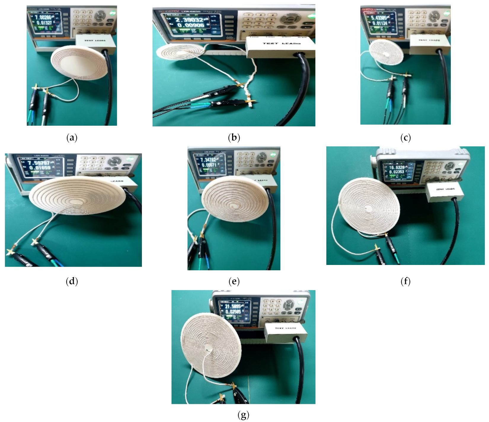
Finally, the calculation results are verified experimentally. The fabricated coils, shown in Figure 2a, are measured with the Gwinstek LCR-6200. Figure 6a–g indicate the measured results. The measured results are compared with the calculation result. The comparison detail is given in

Table 7. Comparison between the proposed and measured self-inductances.

Number of Turns	Calculated Self-Inductance (uH)	Measured Self-Inductance (uH)	Error (%)
6 (large Ri)	6.94	7.00	0.85
7	2.37	2.39	0.83
10 (small Ro)	5.39	5.43	0.73
10 (w = 4.2)	7.26	7.34	1.08
10 (w = 3.6)	7.56	7.59	0.39
15	16.38	16.63	1.50
17	21.46	21.58	0.55

. The calculation result shows a reasonable error below 2%.

There are several self-inductance formulas. Most of them are derived from the Wheeler formula or its modified form. These are obtained empirically in comparison to a proposed method which is derived analytically. Some cases are discussed in this paper.

A coil in Figure 6a has a large inductance value compared to Figure 6b,c, which relatively has a higher number of turns. This shows that inductance depends more on the size than the number of turns for the same turn gap. Moreover, the inductance of the hollow coil is higher than the full coil for a similar size spiral. Because inner turns lie near the center of the spiral coil in the Full coil, it contributes more negative mutual inductance than the positive mutual inductance. Therefore, the overall inductance is decreased.

For many reasons, some conventional formulas do not include the wire diameter parameter which affects the self-inductance. The comparison of Figure 6d,e proves that self-inductance is changed when the wire diameter is modified. The inductance will be larger for smaller wire diameters or vice versa.

In this paper, we assumed that the uniform current is flowing in the spiral coil. However, the self-inductance could be different for the nonuniform current distribution. In this regard, it requires further research. Moreover, the proposed method has a large error for a coil of very small turns and large turn spacing. However, such a coil is not used in most practical applications.

6. Conclusions

In this paper, a new accurate method to calculate the self-inductance of the Archimedean spiral coil is proposed. It is derived by solving the Neumann integral formula. The detailed mathematical derivation of the spiral is presented. The proposed method is solved numerically for several coil geometries considering all the parameters which influence the inductance, such as wire diameter, inner radius, number of turns, outer radius, and turn gap.

To verify its accuracy, it has been compared in three ways: 3D FEM, Wheeler inductance formulas, its modified form and another conventional formula, and finally, by measurement. Utilizing the Wheeler formula or its modified form to calculate the self-inductance, relative to the simulation result, the error increases gradually to more than 40% when the wire diameter decreases. The conventional formula Equation (16) has an exception in this regard. The error does not increase with the decrease in wire diameter. Yet, the error is increased to above 30% when the number of turns of spiral increases. However, the proposed method shows errors below 7% for all cases. Therefore, the validity of our method makes it a good candidate for applications where the self-inductance calculation and designing of spiral coils is required.

References

- Mutashar, S.; Mahammad, A.H.; Salina, A.S.; Hussain, A. Analysis and optimization of spiral circular inductive coupling link for bio-implanted applications on air and within human tissue. Sensors 2014, 14, 11522–11541. [Google Scholar] [CrossRef] [PubMed] [Green Version]
- Jow, U.-M.; Ghovanloo, M. Design and optimization of printed spiral coils for efficient transcutaneous inductive power transmission. IEEE Trans. Biomed. Circuits Syst. 2007, 1, 193–202. [Google Scholar] [CrossRef] [PubMed]
- Duong, T.P.; Lee, J.-W. A Dynamically Adaptable Impedance-Matching System for Midrange Wireless Power Transfer with Misalignment. Energies 2015, 8, 7593–7617. [Google Scholar] [CrossRef] [Green Version]
- Ellis, G.A. Application of the Wheeler Incremental Inductance Rule for Robust Design and Modeling of MMIC Spiral Inductors. ACES J. Appl. Comput. Electromagn. Soc. 2011, 26, 484. [Google Scholar]
- Faria, A.; Marques, L.; Ferreira, C.; Alves, F.; Cabral, J. A Fast and Precise Tool for Multi-Layer Planar Coil Self-Inductance Calculation. Sensors 2021, 21, 4864. [Google Scholar] [CrossRef] [PubMed]
- Nguyen, M.Q.; Hughes, Z.; Woods, P.; Seo, Y.-S.; Rao, S.; Chiao, J.-C. Field distribution models of spiral coil for misalignment analysis in wireless power transfer systems. IEEE Trans. Microw. Theory Tech. 2014, 62, 920–930. [Google Scholar] [CrossRef]
- Waters, B.H.; Mahoney, B.J.; Lee, G.; Smith, J.R. Optimal coil size ratios for wireless power transfer applications. In Proceedings of the 2014 IEEE International Symposium on Circuits and Systems (ISCAS), Melbourne, Australia, 1–5 June 2014; pp. 2045–2048. [Google Scholar]
- Raju, S.; Wu, R.; Chan, M.; Yue, C.P. Modeling of mutual coupling between planar inductors in wireless power applications. IEEE Trans. Power Electron. 2013, 29, 481–490. [Google Scholar] [CrossRef]
- Lockwood, E.H. Book of Curves; Cambridge University Press: Cambridge, UK, 2007. [Google Scholar]
- Wheeler, H. Formulas for the Skin Effect. Proc. IRE 1942, 30, 412–424. [Google Scholar] [CrossRef]
- Chatterjee, S.; Iyer, A.; Bharatiraja, C.; Vaghasia, I.; Rajesh, V. Design Optimisation for an Efficient Wireless Power Transfer System for Electric Vehicles. Energy Procedia 2017, 117, 1015–1023. [Google Scholar] [CrossRef]
- Mohan, S.S.; del Hershenson, M.M.; Boyd, S.P.; Lee, T.H. Simple accurate expressions for planar spiral inductances. IEEE J. Solid-State Circuits 1999, 34, 1419–1424. [Google Scholar] [CrossRef] [Green Version]
- Haerinia, M.; Afjei, E.S. Resonant inductive coupling as a potential means for wireless power transfer to printed spiral coil. J. Electr. Eng. 2016, 16, 68. [Google Scholar]
- Liu, T.; Wei, Z.; Chi, H.; Yin, B. Inductance Calculation of Multilayer Circular Printed Spiral Coils. J. Phys. Conf. Ser. 2019, 1176, 062045. [Google Scholar] [CrossRef]
- Kim, D.-H.; Kim, J.; Park, Y.-J. Optimization and design of small circular coils in a magnetically coupled wireless power transfer system in the megahertz frequency. IEEE Trans. Microw. Theory Tech. 2016, 64, 2652–2663. [Google Scholar] [CrossRef]
- Liu, S.; Su, J.; Lai, J.; Zhang, J.; Xu, H. Precise Modeling of Mutual Inductance for Planar Spiral Coils in Wireless Power Transfer and Its Application. IEEE Trans. Power Electron. 2021, 36, 9876–9885. [Google Scholar] [CrossRef]
- De Queiroz, A.; Carlos, M. Mutual Inductance and Inductance Calculations by Maxwell’s Method. Home Page of Dr. Antonio Carlos M. de Queiroz. 2005. Available online: https://studylib.net/doc/18237615/mutual-inductance-and-inductance-calculations-by-maxwell-s (accessed on 18 December 2021).
- Wheeler, H.A. Inductance formulas for circular and square coils. Proc. IEEE 1982, 70, 1449–1450. [Google Scholar] [CrossRef]
- Wheeler, H. Simple Inductance Formulas for Radio Coils. Proc. IRE 1928, 16, 1398–1400. [Google Scholar] [CrossRef]
- Chan, H.L.; Cheng, K.W.E.; Sutanto, D. A simplified Neumann’s formula for calculation of inductance of spiral coil. In Proceedings of the 2000 Eighth International Conference on Power Electronics and Variable Speed Drives (IEE Conf. Publ. No. 475), London, UK, 18–19 September 2000. [Google Scholar]
- Inan, U.S. Engineering Electromagnetics; Pearson Education India: Delhi, India, 1998. [Google Scholar]
- Wang, X.; Sun, P.; Deng, Q.; Wang, W. Evaluation of AC resistance in litz wire planar spiral coils for wireless power transfer. J. Power Electron. 2018, 18, 1268–1277. [Google Scholar]
- Rossmanith, H.; Doebroenti, M.; Albach, M.; Exner, D. Measurement and characterization of high frequency losses in nonideal litz wires. IEEE Trans. Power Electron. 2011, 26, 3386–3394. [Google Scholar] [CrossRef]
- Vaisanen, V.; Hiltunen, J.; Nerg, J.; Silventoinen, P. AC resistance calculation methods and practical design considerations when using litz wire. In Proceedings of the IECON 2013—39th Annual Conference of the IEEE Industrial Electronics Society, Vienna, Austria, 10–13 November 2013; pp. 368–375. [Google Scholar]
Figure 1.
(a) Archimedean spiral coil. (b) Archimedean spiral coil with its mirror coil.
Figure 2.
Spiral coil. (a) Bobbin (b) Spiral coil with bobbin.
Figure 3.
Measurement of the length of lay.
Figure 4.
(a) Soldering set. (b) Solder failure (solder pot temperature 500).
Figure 5.
Cross cut of the soldered end. (a) Cut of the soldered end. (b) Good soldering (3% difference between calculated and measured resistance). (c) Bad soldering (27% difference between calculated and measured resistance).
Figure 6.
Self-inductance. (a) Six-turn coil having parameters Ri = 85 mm, s + w = 5 mm, w = 3.6 mm. (b) Seven-turn coil, s + w = 5 mm, Ri = 13 mm, w = 3.6 mm. (c) Ten-turn coil, s + w = 5 mm, Ri = 10 mm, w = 3.6 mm. (d) Ten-turn coil, s + w = 7.5 mm, Ri = 10 mm, w = 3.6 mm. (e) Ten-turn coil, s + w = 7.5 mm, Ri = 10 mm, w = 4.2 mm. (f) Fifteen-turn coil, s + w = 5 mm, Ri = 10 mm, w = 3.6 mm. (g) Seventeen-turn coil s + w = 4.41 mm, Ri = 10 mm, w = 3.6 mm.