
Impact of Time-of-Use Demand Response Program on Optimal Operation of Afghanistan Real Power System

 , ,
, ,  , , ,
, , , 
Abstract
:1. Introduction
2. Literature Review
- Investigating the influences of the TOU-DR program on the optimal operation of a large practical power system from the economic and reliability points of view, which are vital issues for Afghanistan.
- Applying a novel two-stage programming on the proposed power system and simulating each stage programming with two cases.
- Making a complete and detailed analysis for the two cases to show the effectiveness and robustness of the proposed control scheme.
- Aiming to attract the attention of policymakers, energy planners, and designers to consider and apply DR programs in Afghanistan’s energy mix.
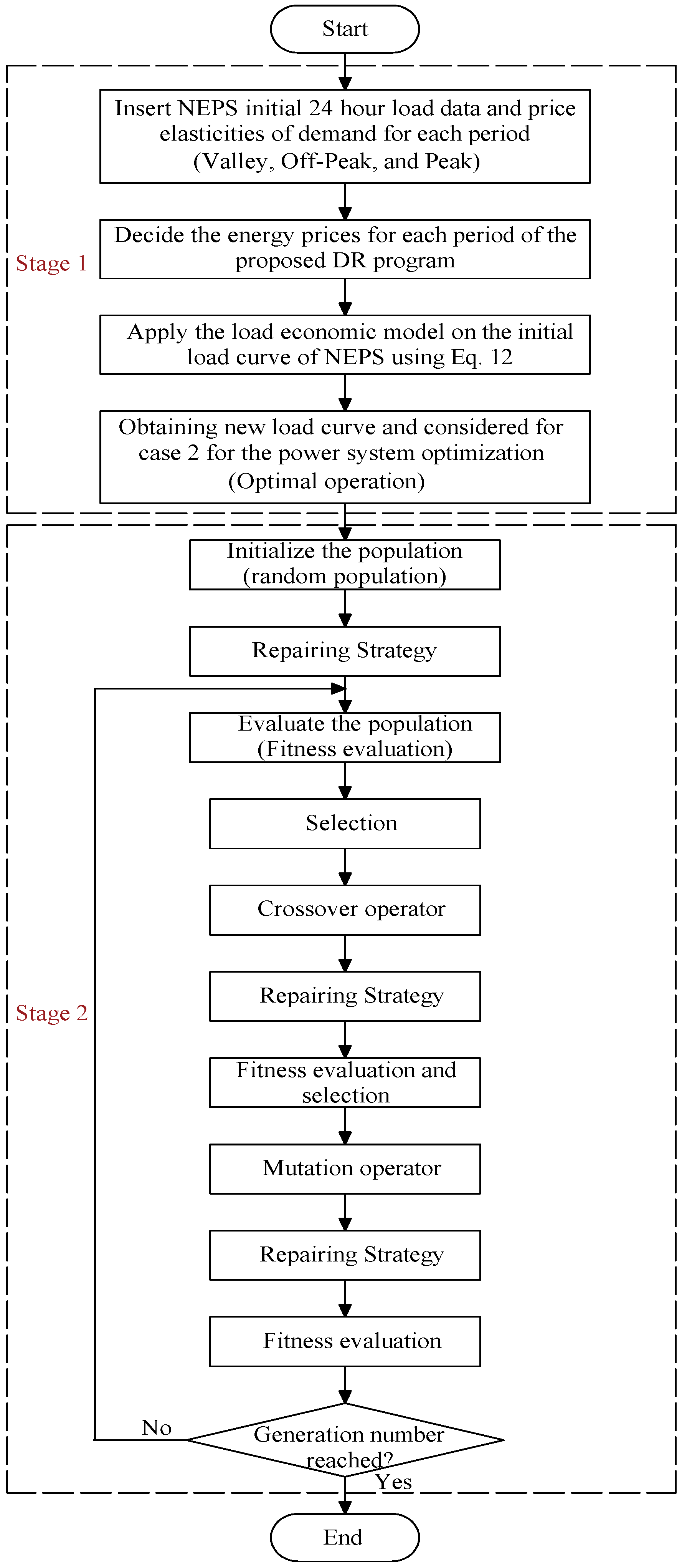
3. Methodology
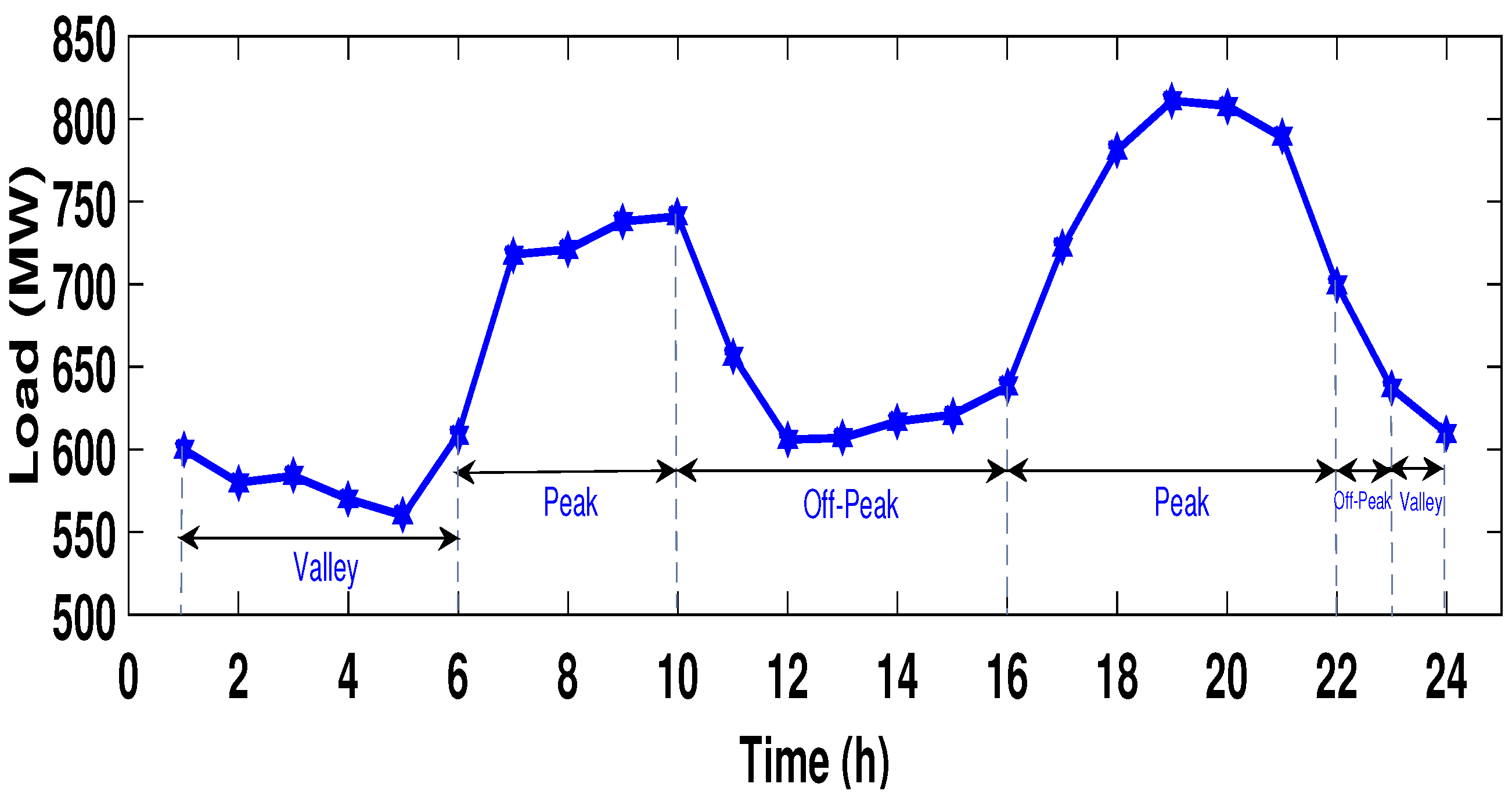
3.1. Stage 1: Modeling of TOU-DR Program
3.2. Stage 2: Power System Formulation and Optimization
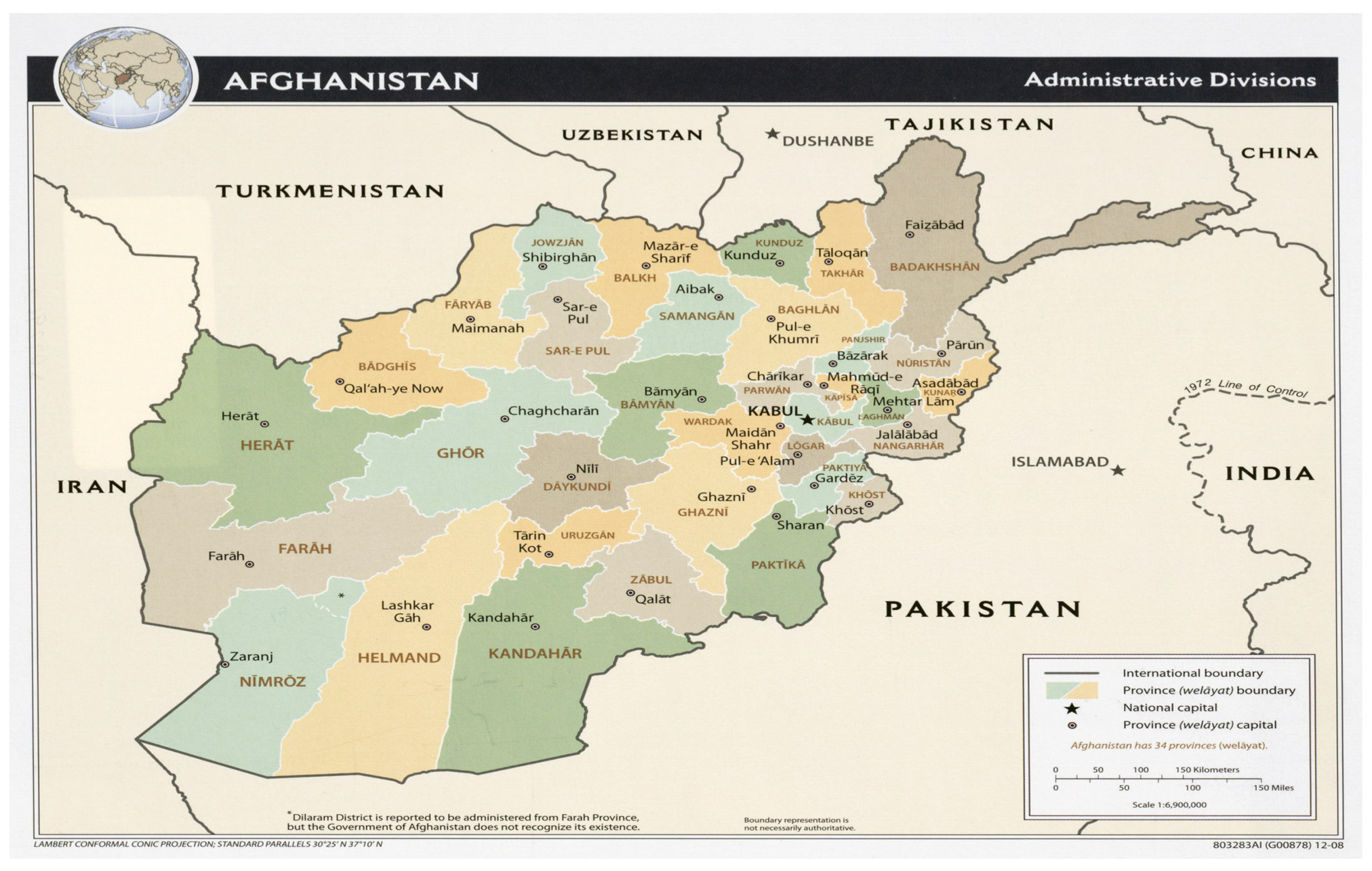
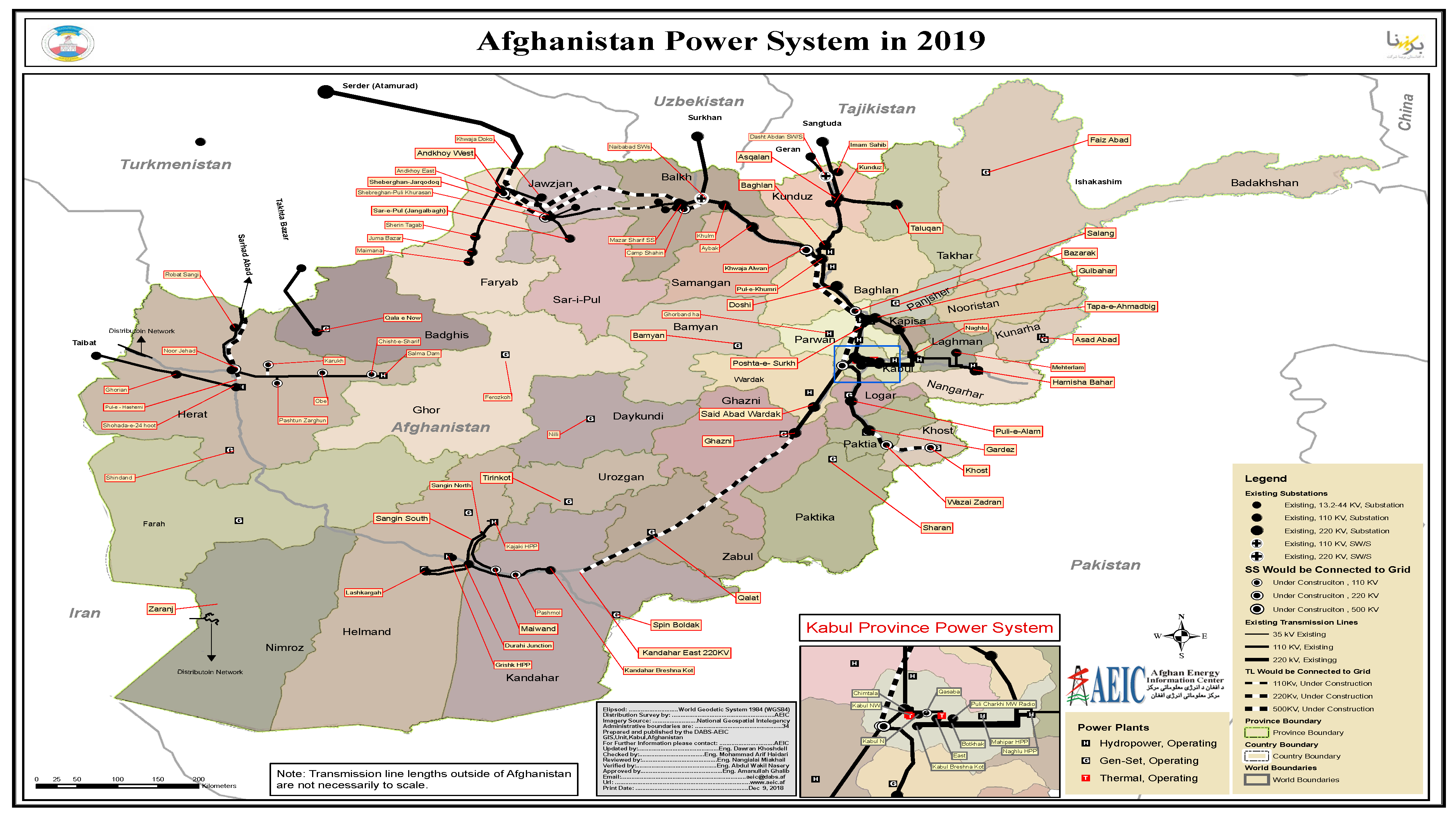
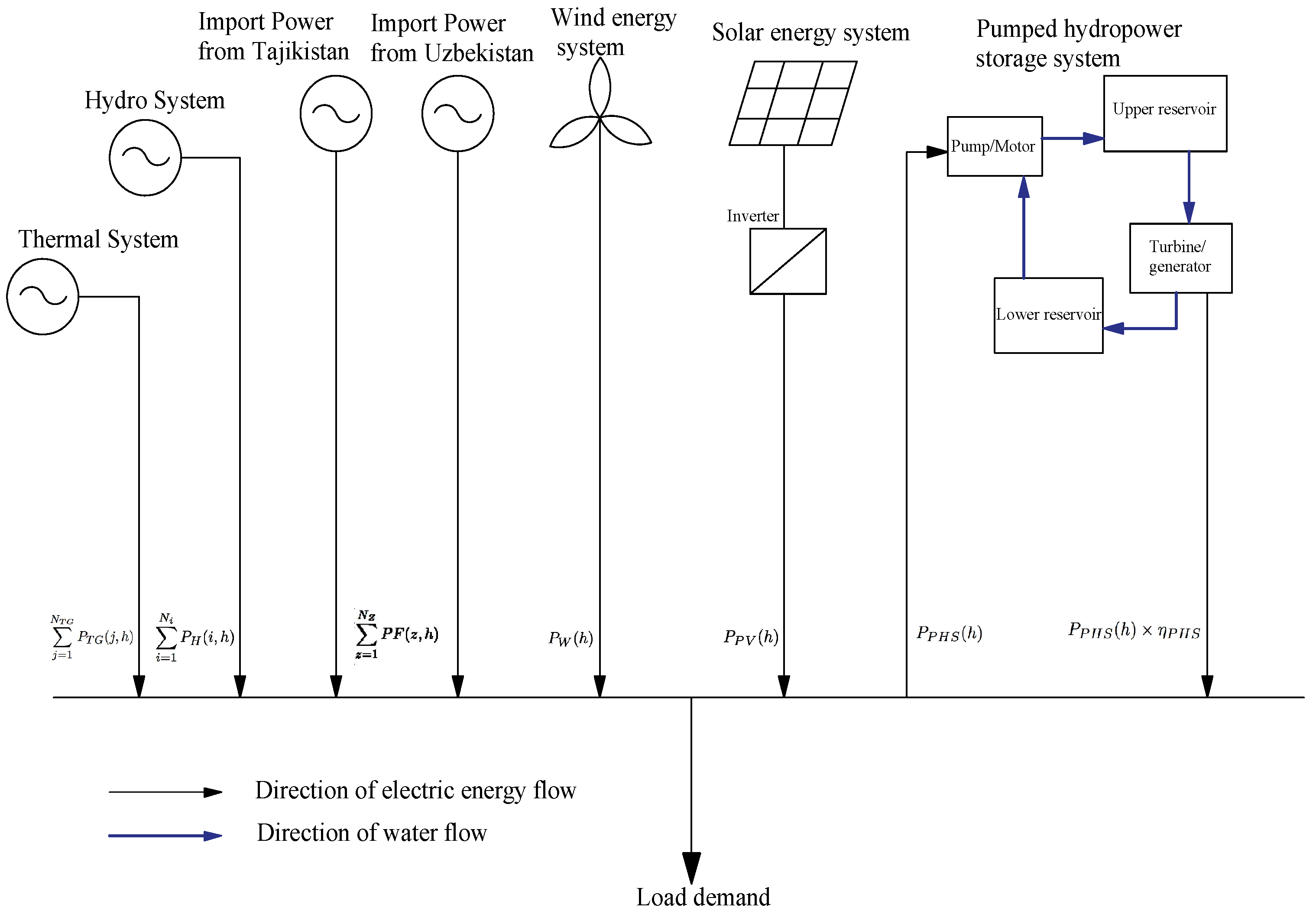
3.2.1. Afghanistan Power System and Its Power Trade with Neighboring Countries
3.2.2. Objective Function
3.2.3. Constraints
Power Balance Constraint
Thermal Units Constraints
Electricity Trading Constraint
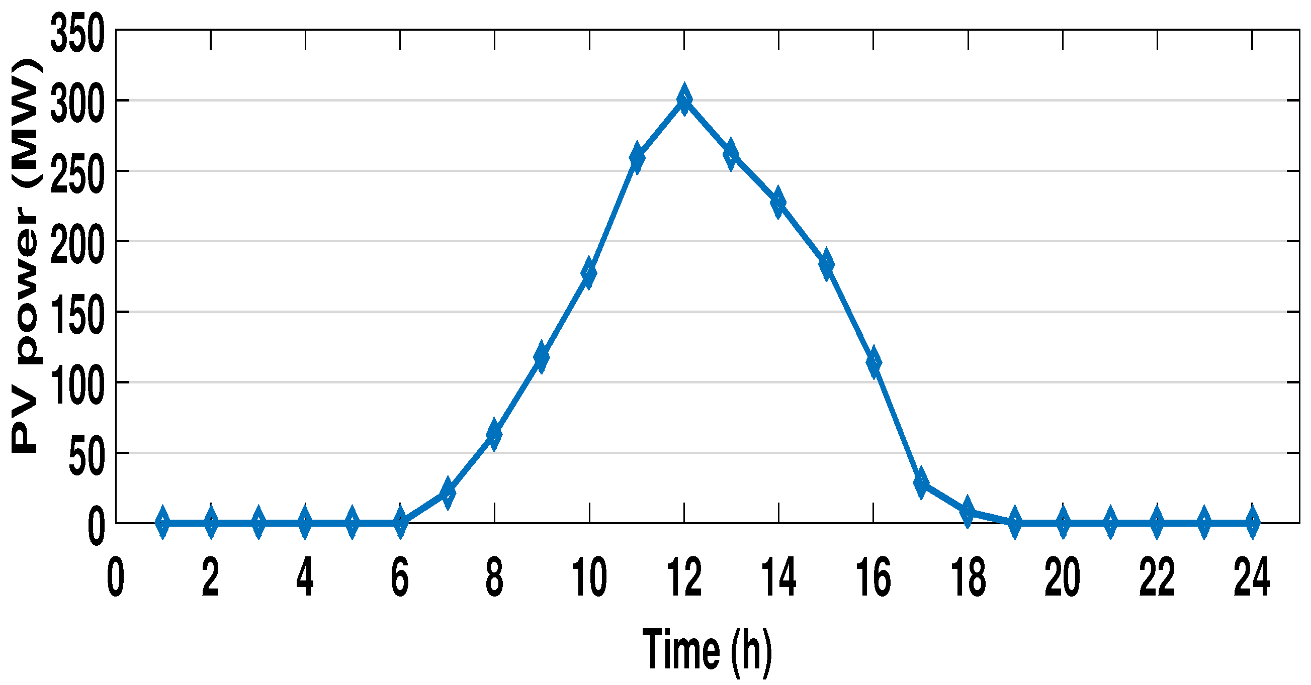
PV Panels Output Power
Wind Generator Output Power
Pumped Hydropower Storage (PHS) Model
4. Binary-Real Coded GA
5. Simulation Test Case
6. Results of TOU-DR Program Implementation and Analysis (Stage 1)
7. Results of Power System Optimization (Stage 2)
8. Results Analysis
9. Conclusions
Author Contributions
Funding
Conflicts of Interest
Abbreviations
| A/S | Ancillary Services |
| DB | Demand Bidding |
| CAP | Capacity Market Program |
| CPP | Critical-Peak-Pricing |
| CPPLC | Critical Peak Load Control |
| DLC | Direct Load Control |
| DR | Demand Response |
| EDRP | Emergency Demand Response Program |
| GA | Genetic Algorithm |
| GDP | Gross Domestic Product |
| GNI | Gross National Income |
| HDI | Human Development Index |
| I/C | Interruptible/Curtailable |
| ILC | Interruptible Load Contract |
| NEPS | Northeast Power System |
| NREL | National Renewable Energy Laboratory |
| PHS | Pumped hydropower storage |
| PV | Photovoltaic |
| Ref. | Reference |
| RESs | Renewable Energy Sources |
| RTP | Real-Time-Pricing |
| TOU-DR | Time-of-Use Demand Response |
| UC | Unit Commitment |
| UNEP | United Nations Environment Program |
| WTs | Wind Turbines |
| Symbol | Description |
| h | Time period, |
| i | Hydropower units, |
| j | Thermal generators, |
| z | Electricity exporting countries, |
| , , | Cost function coefficients of thermal unit j |
| Total area taken by PV array | |
| , | Binary variables [0,1] for pumping/generating modes of PHS |
| Customer benefit at hour h | |
| Exporting country z selling price | |
| Cost function for electric energy generation of jth thermal generator at time h | |
| Reserve deploying cost from jth thermal generator | |
| jth thermal generator’s start up cost at hour h | |
| Elasticity of demand of hth period versus hth period | |
| Customer’s income from the use of of electric energy during hth hour | |
| Load demand of the network at hour h | |
| Load demand of the network after employing DR program. | |
| Minimum uptime of unit j | |
| Minimum downtime of jth generator | |
| Power flow of zth country to Afghanistan at time h | |
| Minimum power flow of zth country to Afghanistan | |
| Maximum power flow of zth country to Afghanistan | |
| jth thermal unit’s power production at time h | |
| Maximum generation limit of jth thermal unit | |
| Minimum generation limit of jth thermal unit | |
| Electric power generation of ith hydropower plant at hour h | |
| Power production of PV at hour h | |
| Power generation of wind turbine at period h | |
| Electric energy supply of PHS plant | |
| Minimum energy supply of PHS plant | |
| Maximum energy supply of PHS plant | |
| Rated output power of wind turbine | |
| Scheduled reserve capacity of jth thermal unit at hour h | |
| Hourly solar insulation | |
| State of charge of the upper reservoir of PHS | |
| Minimum limit of the | |
| Maximum limit of the | |
| Start-up/shut down [0,1] states of jth thermal unit at time h | |
| Total uptime of jth unit | |
| Period of jth unit being continuously off | |
| Cut-in speed of wind generator | |
| Rated speed of wind generator | |
| Cut-off speed of wind generator | |
| Initial electricity price at hour h | |
| PHS overall efficiency |
References
- WorldData.info. Energy Consumption in Afghanistan. 2020. Available online: https://www.worlddata.info/asia/afghanistan/energy-consumption.php (accessed on 15 January 2020).
- Map of the World—Maps of Afghanistan. 2020. Available online: http://www.maps-of-the-world.net/maps-of-asia/maps-of-afghanistan/ (accessed on 1 February 2020).
- National Statistics and Information Authority (NSIA). Population Statistics. 2020. Available online: https://nsia.gov.af/services (accessed on 15 March 2020).
- NEPA & UN Environment. Afghanistan: Climate Change Science Perspectives. National Environmental Protection Agency & UN Environment. 2016. Available online: https://postconflict.unep.ch/publications/Afghanistan/UNEP_AFG_CC_Science_perspectives.pdf (accessed on 10 March 2020).
- Central Intelligence Agency (CIA). The World Fact Book: Afghanistan Economy. 2020. Available online: https://www.cia.gov/library/publications/the-world-factbook/geos/af.html (accessed on 5 February 2020).
- United Nations Development Programme (UNDP). Human Development Report: 2019 Human Development Index Ranking. 2020. Available online: http://hdr.undp.org/en/content/2019-human-development-index-ranking (accessed on 15 February 2020).
- The World Bank Data: Afghanistan. 2020. Available online: http://data.worldbank.org/country/afghanistan (accessed on 20 February 2020).
- The World Bank Data: GDP Per Capita-Afghanistan. 2020. Available online: http://data.worldbank.org/indicator/NY.GDP.PCAP.CD?locations=AF (accessed on 20 February 2020).
- Asian Development Bank (ADB). Proposed Multitranche Financing Facility, Islamic Republic of Afghanistan: Energy Supply Improvement Investment Program. 2015. Available online: https://www.adb.org/projects/47282-001/main (accessed on 25 March 2020).
- Call for Expression of Interest (EOI) for Implementation of 100 MW Grid Connected Renewable Energy Projects in Afghanistan. Ministry of Energy and Water of Afghanistan. 2016. Available online: https://docs.google.com/viewer?a=v&pid=sites&srcid=ZGVmYXVsdGRvbWFpbnxpY2VhZmdoYW5pc3RhbnxneDo2ZmMyZjIzNTcyMmJiZTAx (accessed on 20 March 2020).
- Inter-Ministerial Commission for Energy (ICE). Electricity Supply Yearly Trends. 2020. Available online: https://sites.google.com/site/iceafghanistan/electricity-supply (accessed on 20 January 2020).
- Inter-Ministerial Commission for Energy (ICE). Domestic Generation. 2020. Available online: https://sites.google.com/site/iceafghanistan/electricity-supply/domestic-generation-1 (accessed on 25 January 2020).
- Fichtner. Islamic Repulic of Afghanistan: Power Sector Master Plan. ADB. 2013. Available online: https://rise.esmap.org/data/files/library/afghanistan/Electricity%20Access/Afghanistan_Power%20Sector%20Master%20Plan.pdf (accessed on 5 March 2020).
- World Health Organization (WHO). Indoor Air Pollution. 2020. Available online: https://www.who.int/indoorair/health_impacts/burden_national/en/ (accessed on 10 January 2020).
- United Nations Environment Program (UNEP). 2020. Available online: http://www.unep.org/NEWSCENTRE/default.aspx?DocumentId=2667&ArticleId=9054 (accessed on 5 January 2020).
- Sediqi, M.M.; Furukakoi, M.; Lotfy, M.E.; Yona, A.; Senjyu, T. Optimal economical sizing of grid-connected hybrid renewable energy system. J. Energy Power Eng. 2017, 11, 244–253. [Google Scholar]
- Sediqi, M.M.; Furukakoi, M.; Lotfy, M.E.; Yona, A.; Senjyu, T. An optimization approach for unit commitment of a power system integrated with renewable energy sources: A case study of Afghanistan. J. Energy Power Eng. 2017, 11, 528–536. [Google Scholar]
- Sediqi, M.M.; Furukakoi, M.; Ibrahimi, A.M.; Senjyu, T.; Danish, M.S.S. Multi-objective optimal unit commitment scheme considering renewable energy sources. In Proceedings of the 60th Japan Joint Automatic Control Conference, Tokyo, Japan, 10–12 November 2017; pp. 1–8. [Google Scholar]
- Mohagheghi, S.; Yang, F.; Falahati, B. Impact of demand response on distribution system reliability. In Proceedings of the IEEE Power and Energy Society General Meeting, Detroit, MI, USA, 24–28 July 2011; pp. 1–7. [Google Scholar]
- Conteh, A.; Lotfy, M.E.; Kipngetich, K.M.; Senjyu, T.; Mandal, P.; Chakraborty, S. An economic analysis of demand side management considering interruptible load and renewable energy integration: A case study of Freetown Sierra Leone. Sustainability 2019, 11, 2828. [Google Scholar] [CrossRef] [Green Version]
- Albadi, M.H.; EL-Saadany, E.F. A summary of demand response in electricity markets. Electr. Power Syst. Res. 2008, 78, 1989–1996. [Google Scholar] [CrossRef]
- Baboli, P.T.; Moghaddam, M.P.; Eghbal, M. Present status and future trends in enabling demand response programs. In Proceedings of the IEEE Power and Energy Society General Meeting, Detroit, MI, USA, 24–28 July 2011; pp. 1–6. [Google Scholar]
- Falsafi, H.; Zakariazadeh, A.; Jadid, S. The role of demand response in single and multi-objective wind-thermal generation scheduling: A stochastic programming. Energy 2014, 64, 853–867. [Google Scholar] [CrossRef]
- Jordehi, A.R. Optimization of demand response in electric power systems, a review. Renew. Sustain. Energy Rev. 2019, 103, 308–319. [Google Scholar] [CrossRef]
- Oprea, S.; Bâra, A. Setting the Time-of-Use Tariff Rates with NoSQL and Machine Learning to a Sustainable Environment. IEEE Access 2020, 8, 25521–25530. [Google Scholar] [CrossRef]
- Oprea, S.; Bâra, A.; Ifrim, G. Flattening the electricity consumption peak and reducing the electricity payment for residential consumers in the context of smart grid by means of shifting optimization algorithm. Comput. Ind. Eng. 2018, 122, 125–139. [Google Scholar] [CrossRef]
- Geol, L.; Wu, Q.; Wang, P. Nodal price volatility reduction and reliability enhancement of restructured power systems considering demand-price elasticity. Electr. Power Syst. Res. 2008, 78, 1655–1663. [Google Scholar] [CrossRef]
- Aalami, H.A.; Moghaddam, M.P.; Yousefi, G.R. Modeling and prioritizing demand response programs in power markets. Electr. Power Syst. Res. 2010, 80, 426–435. [Google Scholar] [CrossRef]
- Aalami, H.A.; Moghaddam, M.P.; Yousefi, G.R. Demand response modeling considering interruptible/curtailable loads and capacity market programs. Appl. Energy 2010, 87, 243–250. [Google Scholar] [CrossRef]
- Aalami, H.A.; Moghaddam, M.P.; Yousefi, G.R. Evaluation of nonlinear models for time-based rates demand response programs. Electr. Power Energy Syst. 2015, 65, 282–290. [Google Scholar] [CrossRef]
- Andebili, M.R.; Abdollahi, A.; Moghaddam, M.P. An investigation of implementing emergency demand response program (EDRP) in unit commitment problem. In Proceedings of the IEEE Power and Energy Society General Meeting, Detroit, MI, USA, 24–28 July 2011; pp. 1–7. [Google Scholar]
- Sahebi, M.M.; Duki, E.A.; Kia, M.; Soroudi, A.; Ehsan, M. Simultaneous emergency demand response programming and unit commitment programming in comparison with interruptible load contracts. IET Gener. Transm. Distrib. 2012, 6, 605–611. [Google Scholar] [CrossRef]
- Nikzad, M.; Mozafari, B.; Bashirvand, M.; Solaymani, S.; Ranjbar, A.M. Designing time-of-use program based on stochastic security constrained unit commitment considering reliability index. Energy 2012, 41, 541–548. [Google Scholar] [CrossRef]
- Aghaei, J.; Alizadeh, M. Critical peak pricing with load control demand response program in unit commitment problem. IET Gener. Transm. Distrib. 2013, 7, 681–690. [Google Scholar] [CrossRef]
- Kirchen, D.S.; Strbac, G. Fundamentals of Power System Economics; John Wiley & Sons: Hoboken, NJ, USA, 2019; Available online: https://www.usb.ac.ir/FileStaff/7926_2019-4-10-12-27-43.pdf (accessed on 20 February 2020).
- Data Collected from Energy Engineering Department; Kabul University: Kabul, Afghanistan, 2020; Available online: https://ku.edu.af/energy-engineering-department-0 (accessed on 10 January 2020).
- Aminjonov, F. Afghanistan’s energy security: Tracing Central Asian countries’ contribution. Friedrich-Ebert-Stiftung 2016. Available online: https://library.fes.de/pdf-files/bueros/kabul/12790.pdf (accessed on 15 February 2020).
- Irving, J.; Meier, P. Afghanistan Resource Corridor Development: Power Sector Analysis. Aust. AID. 2012. Available online: https://documents1.worldbank.org/curated/en/161951467989550469/pdf/796990v20WP0P100Box037978900PUBLIC0.pdf (accessed on 10 March 2020).
- Sun, L.; Zhang, Y.; Jiang, C. A matrix real-coded genetic algorithm to the unit commitment problem. Electr. Power Syst. Res. 2006, 76, 716–728. [Google Scholar] [CrossRef]
- Kumar, V.S.; Mohan, M.R. Solution to security constrained unit commitment problem using genetic algorithm. Electr. Power Energy Syst. 2010, 32, 117–125. [Google Scholar] [CrossRef]
- Datta, D. Unit commitment problem with ramp rate constraint using a binary-real-coded genetic algorithm. Appl. Soft Comput. 2013, 13, 3873–3883. [Google Scholar] [CrossRef]
- Sediqi, M.M.; Ibrahimi, A.M.; Danish, M.S.S.; Senjyu, T.; Chakraborty, S.; Mandal, P. An optimization analysis of cross-border electricity trading between Afghanistan and its neighbor countries. IFAC PapersOnLine 2018, 51, 25–30. [Google Scholar] [CrossRef]
- Sediqi, M.M.; Lotfy, M.E.; Ibrahimi, A.M.; Senjyu, T.; Narayanan, K. Stochastic unit commitment and optimal power trading incorporating PV uncertainty. Sustainability 2019, 11, 4504. [Google Scholar] [CrossRef] [Green Version]


| Parameter | Numerical Value |
|---|---|
| Population size | 200 |
| Maximum iteration | 500 |
| Crossover Probability | 0.7 |
| Mutation Probability | 0.3 |
| TG1 | TG2 | TG3 | |
|---|---|---|---|
| [MW] | 105 | 22 | 23 |
| [MW] | 15 | 5 | 5 |
| a [$/h] | 680 | 660 | 665 |
| b [$/MWh] | 16.5 | 25.92 | 27.27 |
| c [$/MW2h] | 0.00211 | 0.00413 | 0.00222 |
| [h] | 4 | 1 | 1 |
| [h] | 4 | 1 | 1 |
| [$] | 560 | 30 | 30 |
| [h] | 4 | 1 | −1 |
| Parameters | Tajikistan | Uzbekistan |
|---|---|---|
| [MW] | 300 | 300 |
| [MW] | 0 | 0 |
| c ($/MWh) | 20 | 60 |
| Hour | (24–6) | (11–16, 23–24) | (7–10, 17–22) |
|---|---|---|---|
| (24–6) | −0.1 | 0.01 | 0.012 |
| (11–16, 23–24) | 0.01 | −0.1 | 0.016 |
| (7–10, 17–22) | 0.012 | 0.016 | −0.1 |
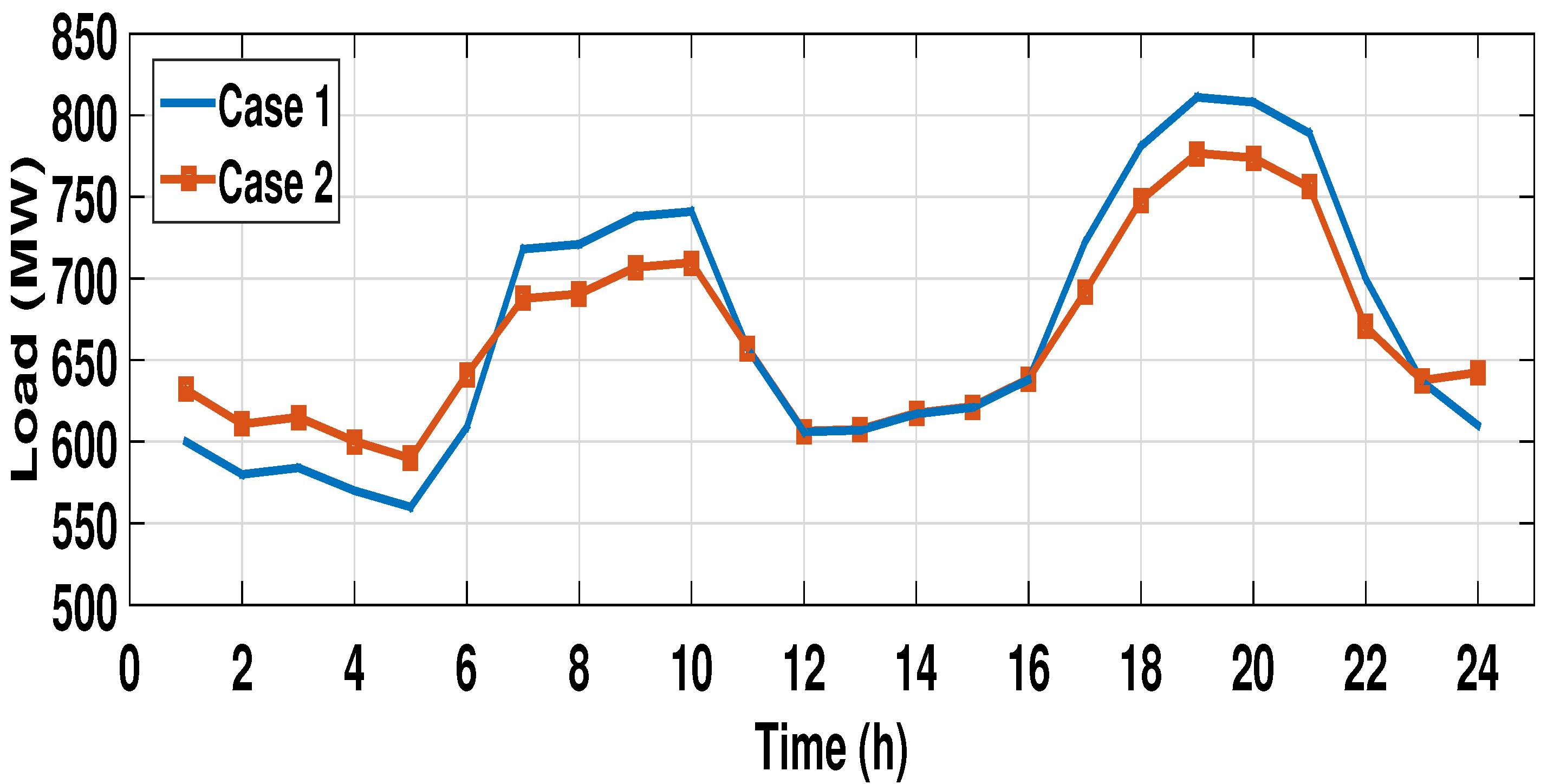
| Parameters | Case 1 (without TOU-DR) | Case 2 (with TOU-DR) |
|---|---|---|
| Energy Consumption (MWh) | 16,025 | 15,930 |
| Customer bill ($) | 528,825 | 512,590 |
| Peak Load (MW) | 811 | 776 |
| Load Factor (%) | 82.33 | 85.53 |
| Customer benefit ($) | 0 | 16,235 |
| Energy reduction (%) | 0 | 0.59 |
| Peak reduction (%) | 0 | 4.31 |
| Peak to valley distance (MW) | 251 | 187 |
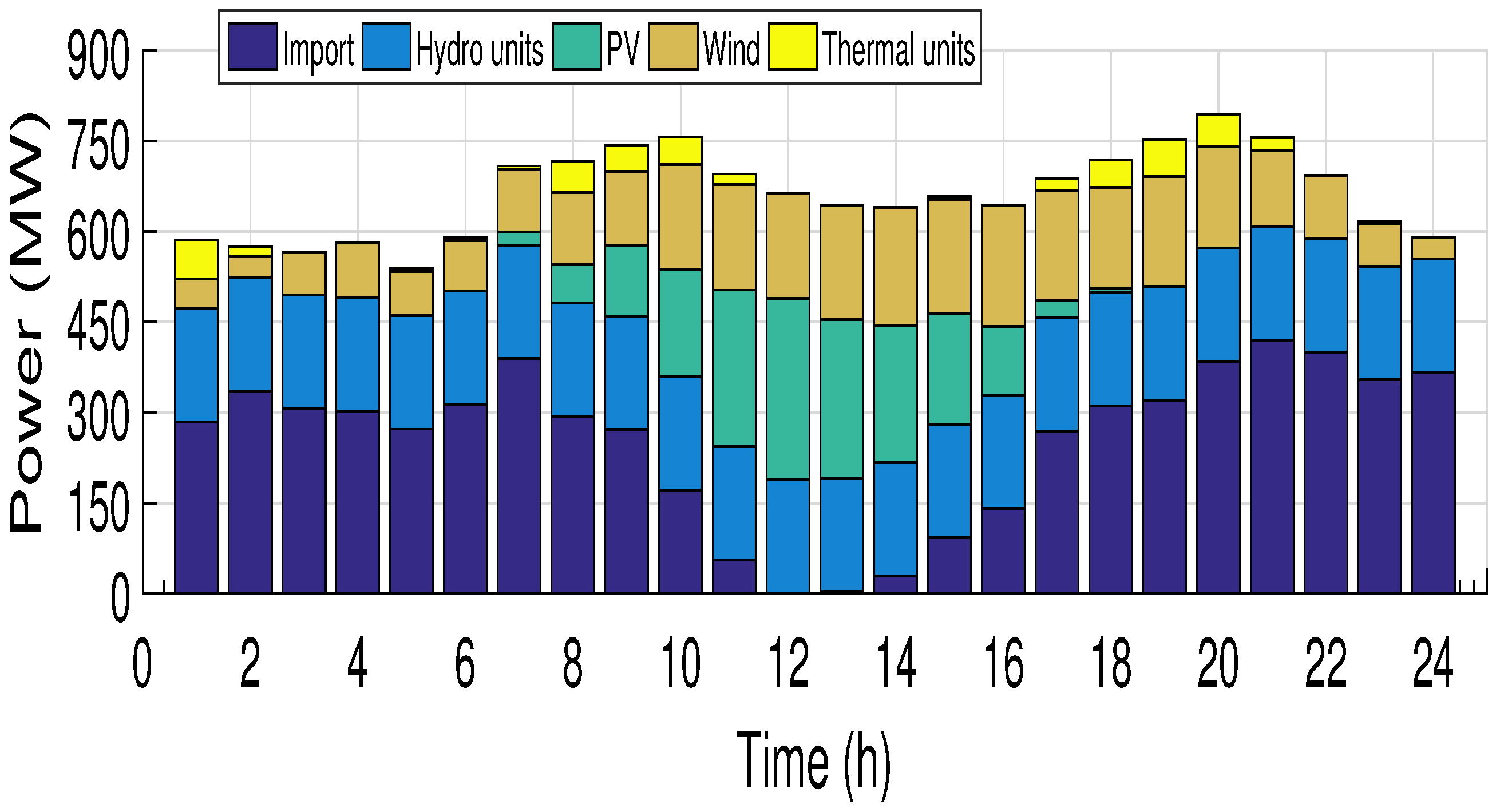
| Parameters | Case 1 (without TOU-DR) | Case 2 (with TOU-DR) |
|---|---|---|
| Total cost ($) | 317,880 | 302,750 |
| Thermal units operation cost ($) | 23,059 | 20,024 |
| Import power tariffs ($) | 238,970 | 228,090 |
| Reserve cost ($) | 55,850 | 54,644 |
Publisher’s Note: MDPI stays neutral with regard to jurisdictional claims in published maps and institutional affiliations. |
© 2022 by the authors. Licensee MDPI, Basel, Switzerland. This article is an open access article distributed under the terms and conditions of the Creative Commons Attribution (CC BY) license (https://creativecommons.org/licenses/by/4.0/).
Share and Cite
Sediqi, M.M.; Nakadomari, A.; Mikhaylov, A.; Krishnan, N.; Lotfy, M.E.; Yona, A.; Senjyu, T. Impact of Time-of-Use Demand Response Program on Optimal Operation of Afghanistan Real Power System. Energies 2022, 15, 296. https://0-doi-org.brum.beds.ac.uk/10.3390/en15010296
Sediqi MM, Nakadomari A, Mikhaylov A, Krishnan N, Lotfy ME, Yona A, Senjyu T. Impact of Time-of-Use Demand Response Program on Optimal Operation of Afghanistan Real Power System. Energies. 2022; 15(1):296. https://0-doi-org.brum.beds.ac.uk/10.3390/en15010296
Chicago/Turabian StyleSediqi, Mohammad Masih, Akito Nakadomari, Alexey Mikhaylov, Narayanan Krishnan, Mohammed Elsayed Lotfy, Atsushi Yona, and Tomonobu Senjyu. 2022. "Impact of Time-of-Use Demand Response Program on Optimal Operation of Afghanistan Real Power System" Energies 15, no. 1: 296. https://0-doi-org.brum.beds.ac.uk/10.3390/en15010296