
Towards a Powerful Hardware-in-the-Loop System for Virtual Calibration of an Off-Road Diesel Engine


1
Energy Department, Politecnico di Torino, Corso Duca degli Abruzzi, 24, 10129 Torino, Italy
2
R&D Department, Lombardini S.r.l.—Kohler Engines, Via Cavaliere del Lavoro Adelmo Lombardini, 2, 42124 Reggio Emilia, Italy
*
Author to whom correspondence should be addressed.
Energies 2022, 15(2), 646; https://0-doi-org.brum.beds.ac.uk/10.3390/en15020646
Submission received: 30 October 2021
/
Revised: 5 January 2022
/
Accepted: 11 January 2022
/
Published: 17 January 2022
(This article belongs to the Special Issue Advanced Calibration Methodologies for a New Generation of Engines and Powertrains)
Abstract
:A common challenge among internal combustion engine (ICE) manufacturers is shortening the development time while facing requirements and specifications that are becoming more complex and border in scope. Virtual simulation and calibration are effective instruments in the face of these demands. This article presents the development of zero-dimensional (0D)—real-time engine and exhaust after-treatment system (EAS) models and their deployment on a Virtual test bench (VTB). The models are created using a series of measurements acquired in a real test bench, carefully performed in view of ensuring the highest reliability of the models themselves. A zero-dimensional approach was chosen to guarantee that models could be run in real-time and interfaced to the real engine Electronic Control Unit (ECU). Being physically based models, they react to changes in the ECU calibration parameters. Once the models are validated, they are then integrated into a Simulink® based architecture with all the Inputs/Outputs connections to the ECU. This Simulink® model is then deployed on a Hardware in the Loop (HiL) machine for ECU testing and calibration. The results for engine and EAS performance and emissions align with both steady-state and transient measurements. Finally, two different applications of the HiL system are presented to explain the opportunities and advantages of this tool integrated within the standard engine development. Examples cited refer to altitude calibration activities and soot loading investigation on vehicle duty cycles. The cases described in this work are part of the actual development of one of the latest engines developed by Kohler Engines: the KDI 1903 TCR Stage V. The application of this methodology reveals a great potential for engine development and may become an essential tool for calibration engineers.
1. Introduction
Modern off-road diesel engines have to meet many different requirements, including high performance, low fuel consumption and low pollutant emissions, good durability and low total cost of ownership. New legislation framework has extended the emission compliance test to critical areas of the engine operating map, also including extreme ambient conditions, such as very low or high temperatures or high altitudes [1]. The need to comply with these more stringent legislation targets, while achieving at the same time the high-performance goals which are essential for customer acceptance, has significantly increased the system complexity and made the development of the new generation of powertrain extremely challenging. In fact, in recent years, different and innovative technologies such as variable compression ratio [2], variable valve timing [3], multistage boosting systems [4], advanced combustion systems [5,6], high-injection pressure systems [7], advanced injection strategies [8,9] and innovative Exhaust Aftertreatment Systems (EASs) [10] are being developed to improve diesel internal combustion engines (ICEs) efficiency and to reduce pollutants. Therefore, modern diesel ICEs feature very complex control strategies and hardware solutions. Thus, defining an engine’s calibration is an extremely challenging task since it requires the definition of a large number of control parameters to fulfill competing targets such as emissions and fuel consumption. The situation is even more complex for off-road applications of diesel engines because the multiplicity of the customers’ product ranges requires customization of the calibration to optimize the control of the great variety of vehicle variants (excavators, tractors, skid steer loaders, etc.) that leads to a rising number of prototypes for validation and calibration works. The goal of a current development process is to reduce development time and costs by averting time-consuming development loops and exploiting synergies between the derivative developments as far as possible. Nowadays, modern products need to be brought to market cost-effective, with the necessary quality, and within a short development time [11].
Therefore, to have time and cost-effective solutions to deal with the above-mentioned challenges, virtualization becomes mandatory throughout the development process. Several authors have shown that frontloading through detailed and fast virtualization of a powertrain permits a massive reduction of the required test loops on prototype engines [12,13]. Thus, expensive, and time-consuming experimental testing can be easily reduced.
In this context, X-in-the-Loop (XiL) based approaches represent a good solution to move the assessment of design choice and the tuning and calibration process much earlier in the development process. The term “XiL” covers different in-the-loop applications, including, but not limited to, hardware-in-the-loop (HiL), model-in-the-loop (MiL), and software-in-the-loop (SiL). HiL simulation is used commonly in the ICEs industry for different applications; several studies have already highlighted the profit from utilizing HiL based virtualization especially in the automotive field [14,15,16,17]. The key advantage derives from the connection between real systems and physical-based models. The simulative approach by itself has obstacles for seamless system level validation in real duty cycles and extended environmental conditions. The MiL simulation of the Electronic Control Unit (ECU) algorithms in a virtual environment could be a good solution for some development use cases [18], but it needs important effort to set up the control and diagnostic models. Otherwise, a simplified ECU model, which includes generic control logic, may be applied for certain development use cases. The other applicable XiL approaches are the SiL simulation [19] and the virtual ECU based method using the chip simulation [20]. The latter two approaches, however, need an extended exchange of fundamental information (for example c-code or map file) between an Original Equipment Manufacturer (OEM) and participating suppliers (function and software (SW) developers). The HiL system provides a strong solution for an ECU calibration platform [21] and, compared to other X in the loop applications, it grants an excellent trade-off between the effort for testing set-up and the reproducibility of testing conditions [22].
To enhance the system-level understanding of ECU software and complex powertrain at different development steps, the HiL-based virtual calibration approaches are a solution for parametrization of ECU functions and integration of calibration and functional updates. The HiL environment helps to manage hardware changes, requirement changes, software releases as well as complex interactions of many control functions and to validate powertrains derivatives as reported in [22]. The authors have transferred these advanced, future-oriented virtual calibration methods into the standard calibration process and this article will provide, through different case studies, an overview of the key success factors and experiences made along the way.
To support the above tasks, it is necessary to accomplish the real time constraints in the hardware in the loop system: this means that the mean computational time must be less than the system physical time and also that each time step must complete in the given time frame [23]. According to [23], to enable adequate time for the data exchange, the Central Processing Unit (CPU) time of each time step should be shorter than half of the time step itself; thus, Mean Value Engine Model (MVEM) methods are nowadays used [24,25,26,27]. Basically, these approaches combine gas path models based on physics with alternative methods to model the ICE cylinders block. In the MVEMs, the cylinder operation is characterized by a cycle averaged process for enthalpy, mass and species through the cylinders [28]. This is achieved with the introduction of a mean value surrogate engine block model [29,30]. Since MVEMs are not able to capture wave propagation in the manifolds [30,31], special inputs are commonly introduced to consider non-modelled unsteady effects in order to predict more accurate mean flows.
When dealing with HiL applications, explicit methods are generally used to integrate the system of ordinary differential equations which characterizes the system, as they are able to meet the real-time speed of execution constraints when applied together with the proper modeling depth and a suitable set-up of the model. The model stability can be reinforced through the utilization of a transient momentum balance equation in the mean value engine model transfer elements [32]. The MVEM modelling approach needs lower computational effort than the crank-angle resolved model [33]. The combination of MVEMs with a few essential experimental parameters and a high degree of physical principles is used to accomplish acceptable precision while fulfilling the strong real-time constraints. Few examples of the application of such kinds of models for virtual calibration are available in the literature [12,34] and often they are limited to the single subsystem (engine) not considering the interaction with exhaust after-treatment system as shown in this article.
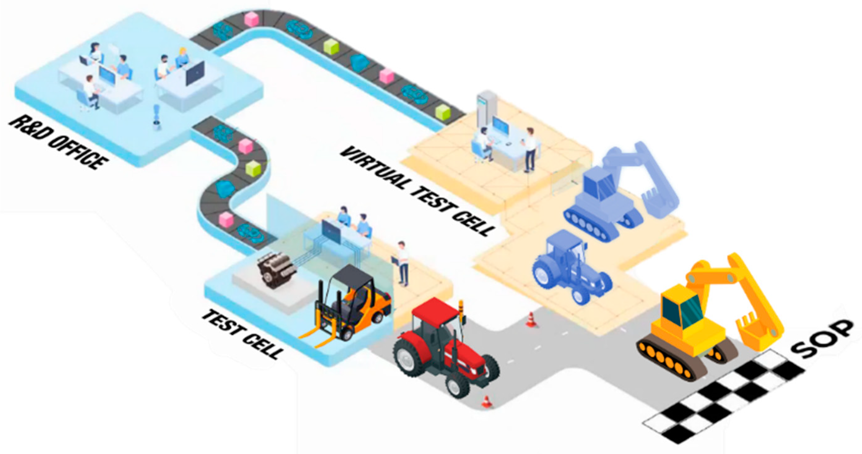
This research aims to prove the support that the HiL system gives during the engine calibration development and to describe its impact on a standard development process. During the calibration development process, the exploitation of simulation tools is not new, but in the case reported in this article an ICE and EAS simulation is regularly applied along with the standard development process. The purpose is to create a development setting that enables the shifting of major development tasks away from the pricey real to the low-cost virtual ICE and EAS testing (Figure 1). In more detail, the authors will show how, exploiting the predictive capabilities of a real-time diesel engine and after-treatment models integrated within the HiL system, it is possible to optimize engine calibration over different ambient conditions and different duty cycles, moving engine calibration much earlier in the engine development process.
2. Materials and Methods
2.1. Virtual Test Bed
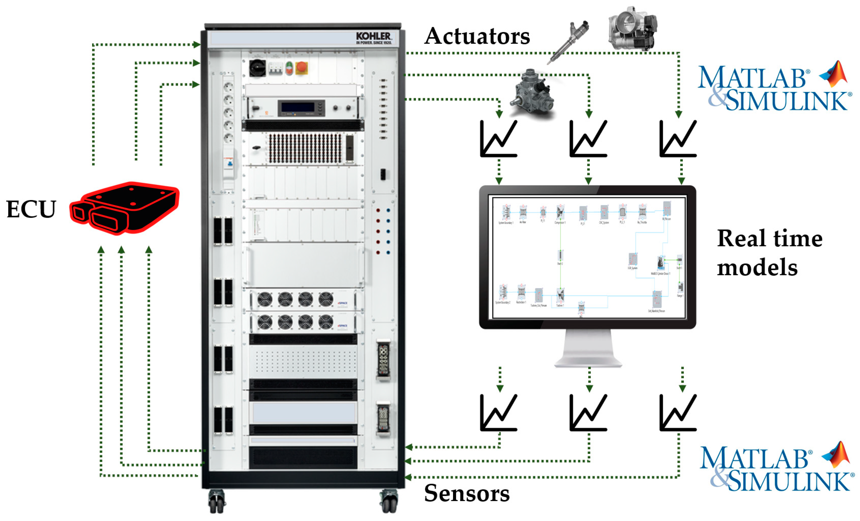
Virtual calibration is a relatively new concept used in the ICEs industry. It is accomplished by using a simulation model and then integrating it with hardware components in a virtual test bed (VTB) (Figure 2). The hardware controller sends actuators’ signals to the simulation model and receives back from the latter the sensor signals, creating a closed-loop environment. Some actuators (e.g., common rail injectors) can be integrated as real components into the HiL simulator and located in a load drawer, since they are quite difficult to be modeled. In this study, the real hardware (HW) components which are contained in the HiL system are listed in Table 1:
The virtual test bench has been developed as a digital twin of a real test bench. This ensures to calibration engineers an easy shift from the real engine testing environment to the virtual testing environment.
The most important keys to performing successful model-based calibration are engine and exhaust after treatment simulation models that must be integrated within the VTB.
2.2. Reference Engine
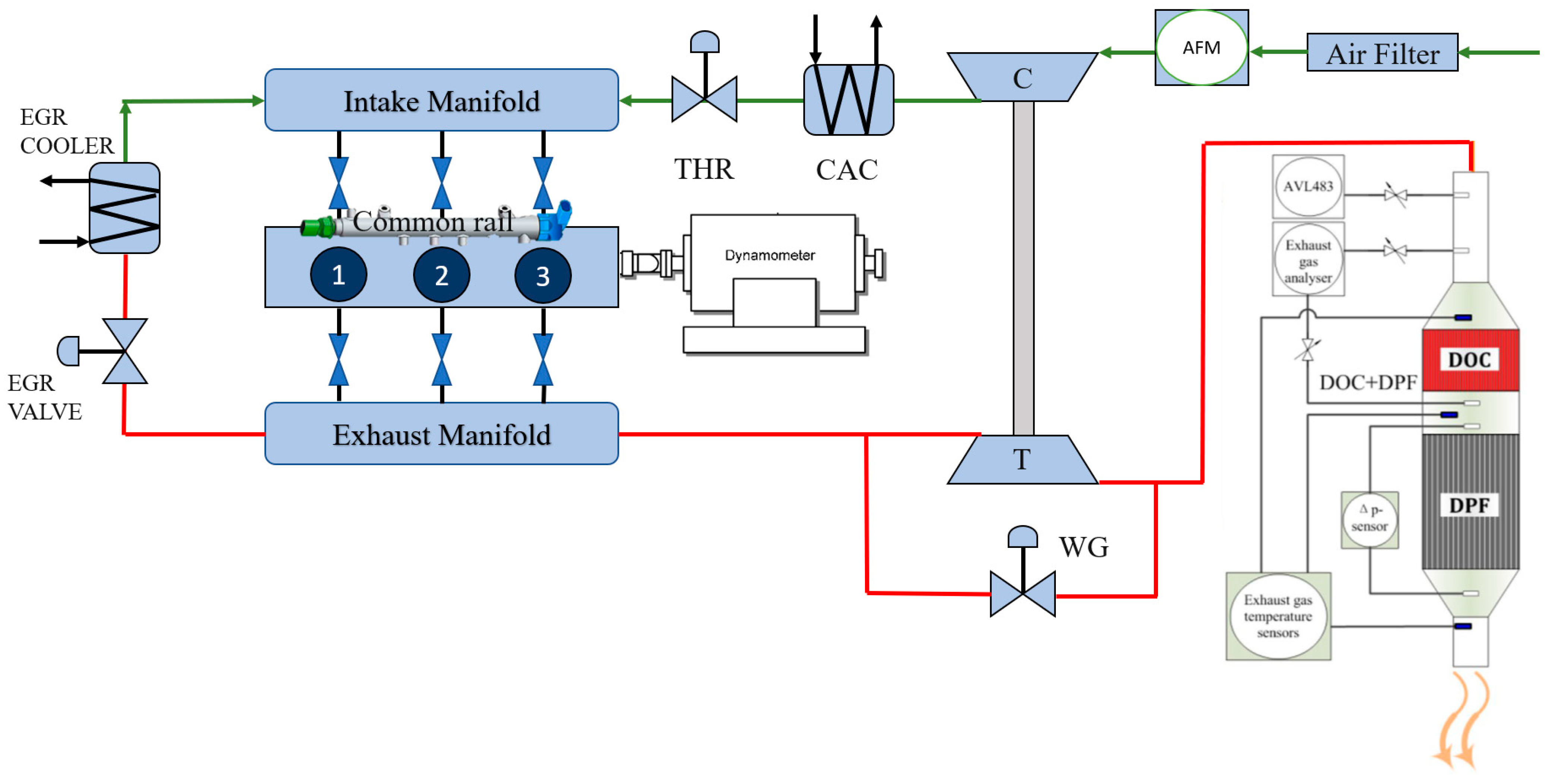
For the given research, a KDI 1903 TCR has been used: a state-of-the-art 1861 cm3 intercooled, turbocharged, three-cylinder, direct injection (DI) diesel engine with Exhaust Gas Recirculation (high-pressure EGR circuit) (Figure 3), developed and manufactured by Kohler Engines.
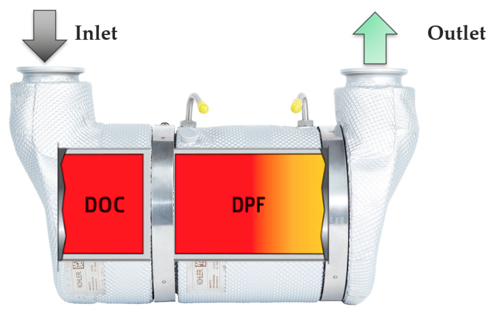
This engine has been developed for Off-Road applications and it is Stage V emission regulations compliant [35]. The engine is equipped with a dedicated EAS composed of a Diesel Oxidation Catalyst (DOC) and a coated Diesel Particulate Filter (cDPF). Engine and EAS specifications are listed in Table 2 [36].
Table 3 contains the specifications of the experimental measurement facility used in the dynamometer test bed for models’ validation.
The raw engine-out gaseous emissions such as HC, CO, CO2, O2, and NOx/NO are measured using an AVL AMA i60 SII. A Mettler-Toledo KA32s bench scale is used for the measurement of the soot mass trapped in the DPF; this instrument has an accuracy of ±0.1 g and a maximum weighing capacity of 30 kg. An AVL 483 micro soot sensor is instead adopted as a measurement system for soot emission concentrations in the exhaust gas coming from the ICE. A representation of the experimental setup used for this article is shown in Figure 3. The tested ICE is instrumented with three thermocouples and a delta pressure sensor in the EAS to record exhaust gas temperature and pressure signals at the highlighted positions.
2.3. Real-Time Engine Model
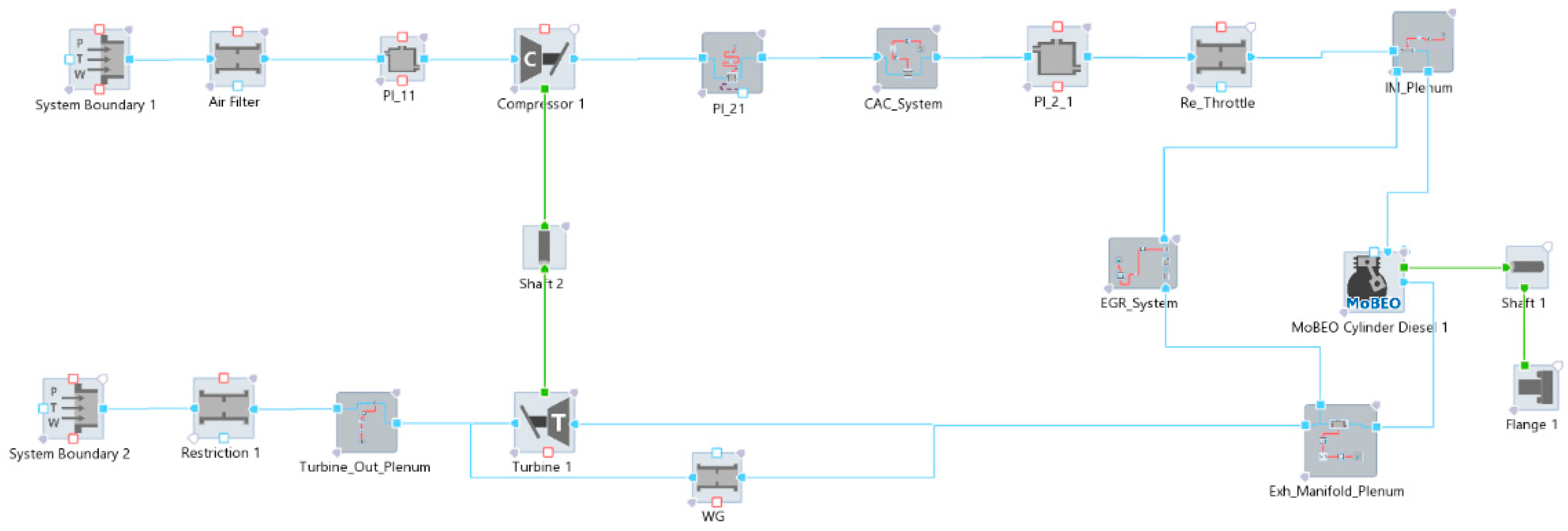
The engine is modelled using a zero-dimensional (0D) mean value approach [37] within the commercially available software AVL CRUISE M™ with MoBEO (model-based engine optimization) libraries, which integrates physical and empirical models (Figure 4): the airpath of the modeled ICE was totally physical, while the cylinder model was based on a semi-physical modeling approach. MoBEO allows concept model capability instead of complex cylinder configurations: the in-cylinder processes are tuned using fit parameters based on a huge amount of engine test bed data. Then, MoBEO demands basic cylinder and fueling parameters coming from the test bench to perform the combustion refinement based on previously embedded measurements. An additional part of this semi-physical approach is made of the engine-out emission models.
Therefore, in order to take into account the effect of different engine calibration parameters such as rail pressure, Start of Injection (SOI), pilot injection, EGR rates and operating conditions on combustion, MoBEO combustion libraries were applied. The MoBEO model divides the in-cylinder content into three thermodynamic zones, each with its own composition and temperature. The main unburned zone is made of all trapped mass at intake valve closure. The spray is separated into two main parts, i.e., burned and unburned zones. The former contains the product of the combustion process, and the latter includes the fuel and entrained gas. The model considers fuel evaporation, mixing, and burning process. The sub-model defining the combustion contains three calibration multipliers:
- Pressure at start of injection correction (PSOIC).
- Combustion delay correction (CDC).
- MFB (mass fraction burned) 50% correction (MFBC).
The following measurements were carried out at Engine Test Bed (ETB) to find the optimum calibration parameters to minimize the Root Mean Squared (RMS) error between experimental and simulated combustion results:
- One engine map using only main injection and without Exhaust Gas Recirculation (EGR) to better estimate the injection delay and engine volumetric efficiency.
- One engine map with standard calibration for overall model parametrization.
Optimized values of the above calibration parameters (PSOIC, CDC, MFBC) are revealed in Table 4.
The NOx calculation is based on the extended Zeldovich mechanism, and it is embedded in the MoBEO cylinder code. Two calibration parameters are used to tune the NOx emissions:
The second step for calibrating the engine model is to parametrize the restrictions and the plenums. Restrictions are transfer components and they have been modelled using basically orifice equations [28] considering a nominal reference area (Aref) and parametrizing the flow coefficient (FC) with test bed data; mass flow () depends on the conditions upstream the restriction (temperature Tin and pressure pin) and pressure downstream the restriction (pout):
In Equation (1), Rin is the upstream specific gas constant. β is a flow function depending on the gas specific heat ratio (k) and on the pressure ratio (pout/pin) across the restriction and it changes for subsonic or sonic flow conditions as:
for subsonic flow and:
for sonic flow.
In similar manner, the velocity in the orifice (uor) is evaluated as:
where “v” is obtained by Equation (5):
for subsonic flow and by:
for sonic flow.
The dependency of the flow coefficient on the pressure ratio or mass flow throughout the resistive component itself is generally parametrized knowing both the mass flow rate at different stationary engine points and the condition upstream and downstream the restriction.
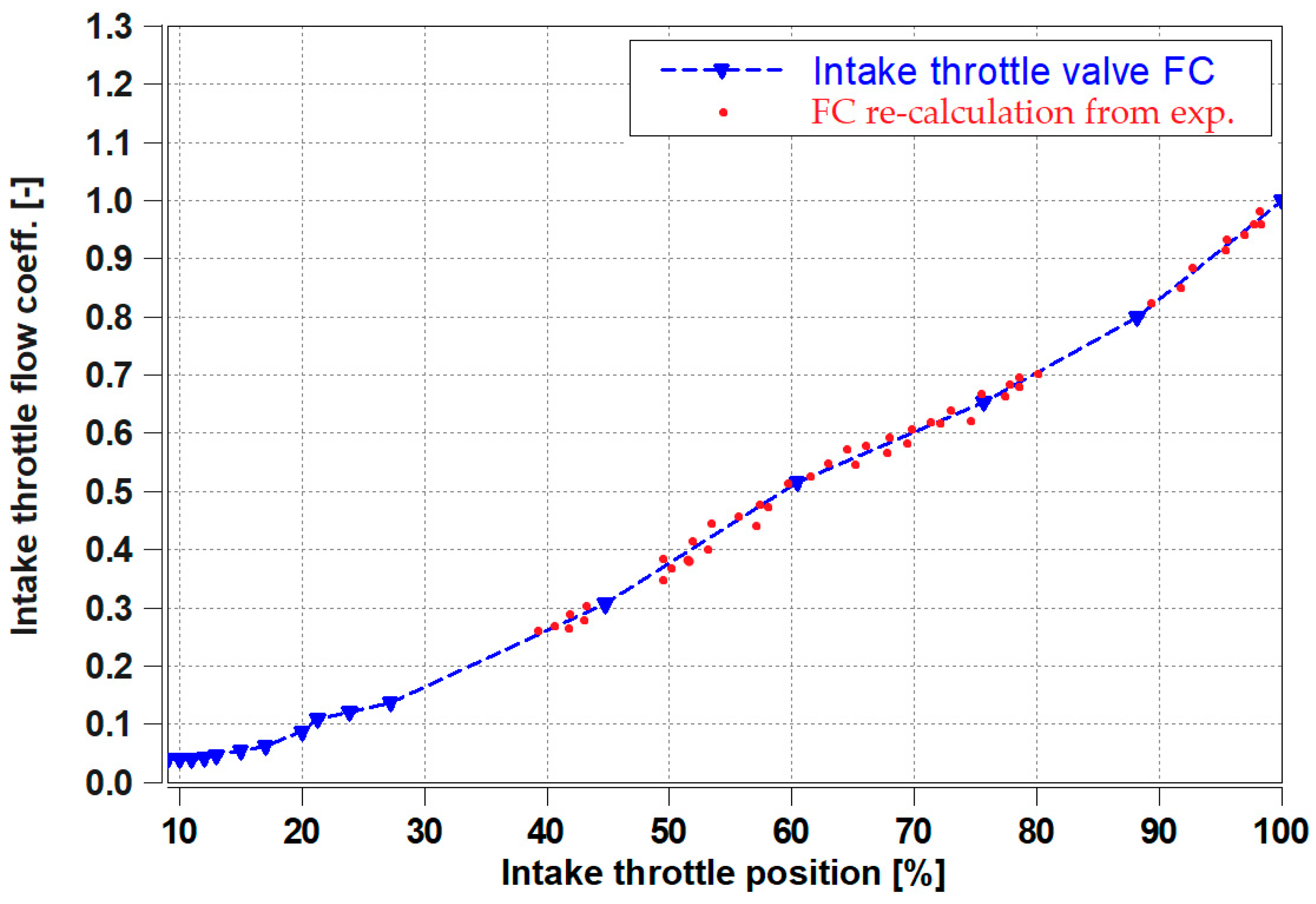
Elements with a variable flow area (for example intake throttle valve and EGR valve) were modeled as restrictions as well, with a fixed nominal area (equal to the maximum nominal area) and a flow coefficient function of the valve opening angle. Figure 5 shows the flow coefficient parametrized on measured data and used for the intake throttle valve in the engine model. The blue curve represents the flow coefficient used to parametrize the intake throttle valve pressure drop. On the other hand, the red points in the chart represent the punctual values of the flow coefficient, recalculated in each stationary engine operating point. Furthermore, the blue curve has been extended to lower and higher values of the throttle valve opening percentage than those available experimentally, to avoid numerical instabilities during simulations.
A plenum, instead, is a volume component that contains gas. During the engine simulation process, it is filled up and emptied with fresh air or exhaust gases thanks to mass balance equation, energy and species concentration, and state equation calculation. The classic species balance equations [38] are considered to reproduce the influence of the gas composition on the fluid physical properties for the whole ICE operating map such as different exhaust gas recirculation and different exhaust gas temperatures: this method is necessary to model the states in the storage elements and the flow through the transfer elements. As described in [39], the classic species approach is useful to reduce the computational cost. Thus, conservation equations for combustion products and fuel vapor are solved. The air mass fraction (µair) is linked to the fuel vapor mass fraction (µfv), the combustion products mass fraction (µcp) and the burned fuel mass fraction (µfb) through the following equation:
The air to fuel ratio (AFCP) is a characteristic quantity that describes the composition and the properties of the combustion products, and it is evaluated by the Equation (8):
The combustion gases composition is calculated from the chemical equilibrium considering dissociation at the high temperatures inside the cylinder. The heat transfer towards the environment was modelled, starting from each plenum, by building a thermal path. This path structure consists of two parts: a convective heat exchange between the solid wall and the gas within the volume, and a convective heat transfer between the environment and the solid wall. The Heat Transfer Coefficient (HTC) between the environment and the solid wall was estimated according to literature values and in particular to [39], whereas the convective heat transfer () between the solid wall and the gas in the plenum, is calculated from the convective law, assuming a constant wall temperature (Tw) and a constant gas temperature (Tgas), according to Equation (9):
where represents a heat transfer multiplier, is the heat transfer surface and HTC represents the convective heat transfer coefficient. This latter is evaluated through the Reynolds analogy [40] and finally tuned acting on the heat transfer multiplier .
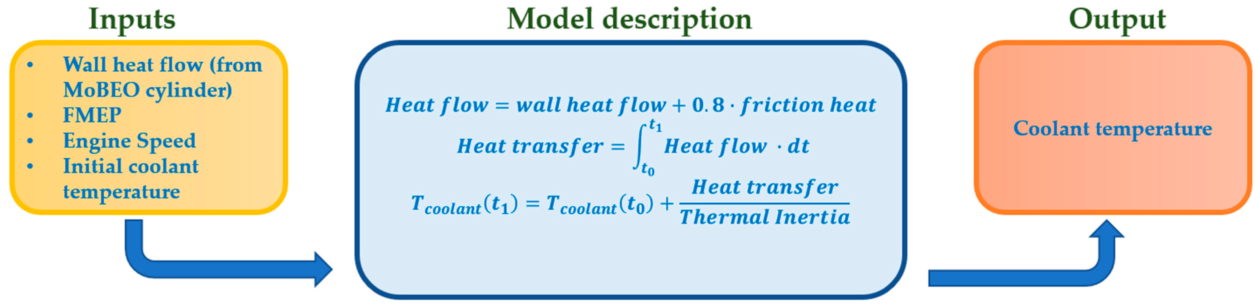
Another important aspect of the engine model is the prediction of the coolant temperature behavior during the warm-up phase because a lot of ECU strategies are based on that temperature. The transient evolution of the coolant temperature is evaluated taking into consideration that in the coolant circuit, the temperature derivative is proportional to the heat flux divided by systems thermal inertia (Figure 6) [39]. When the simulated temperature reaches the target thermostat temperature, a saturator signal is activated.
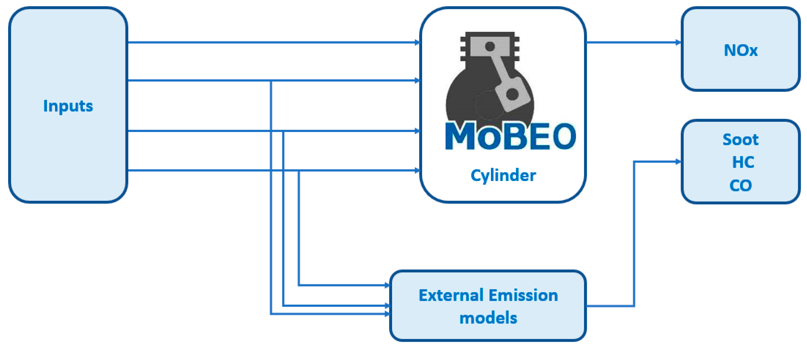
The last step of the ICE model calibration is represented by the engine out emission models. The engine-out nitrogen oxides (NOx) emissions are estimated by a semi-physical model implemented within the cylinder code and parametrized during the combustion process modelling. For Carbon monoxide (CO), Hydrocarbon (HC) and Soot emissions instead, no such models are present since they are strictly engine dependent. External emission models need to be added to the cylinder block (Figure 7).
Therefore, a specific design of experiments (DoE) program was delineated to create a user-defined emission models based on empirical correlations. Since the Soot, HC and CO models are built based on measurement data it is necessary to choose physical approach inputs and not measured parameters. In this way, models’ strength in extrapolation areas is guaranteed. For example, the EGR rate is not taken into account as a model input but the oxygen concentration on the intake mass flow to the cylinder is considered. Moreover, it is necessary to keep as few model inputs as possible without compromising the accuracy of the results to ensure real-time calculation.
For this reason, to implement such correlations two ways have been considered: neural networks and polynomials; neural networks promise a very good fit to measure points, they have very weak extrapolation capabilities, and need a very significant calculation effort (frequently not real-time capable) and must be treated as “black box” model unsuitable to being manipulated in order to replicate expected trends. On account of the above shortcomings, polynomial models were chosen instead, and they were generated using an optimization tool. The structure of each user-defined emission models consists of polynomials with terms up to fifth order and includes cross interactions up to fourth order as described in [39]. The output of these kinds of models is a function of the engine speed, the oxygen content in the cylinder, the rail pressure, the injections timing, the air to fuel ratio and the exhaust mass flow. Dependencies on other engine parameters were ignored since they were deemed less important in agreement with the significance method. An example of used polynomial function considering, for simplicity, only two inputs (x1, x2), is shown in Equation (10):
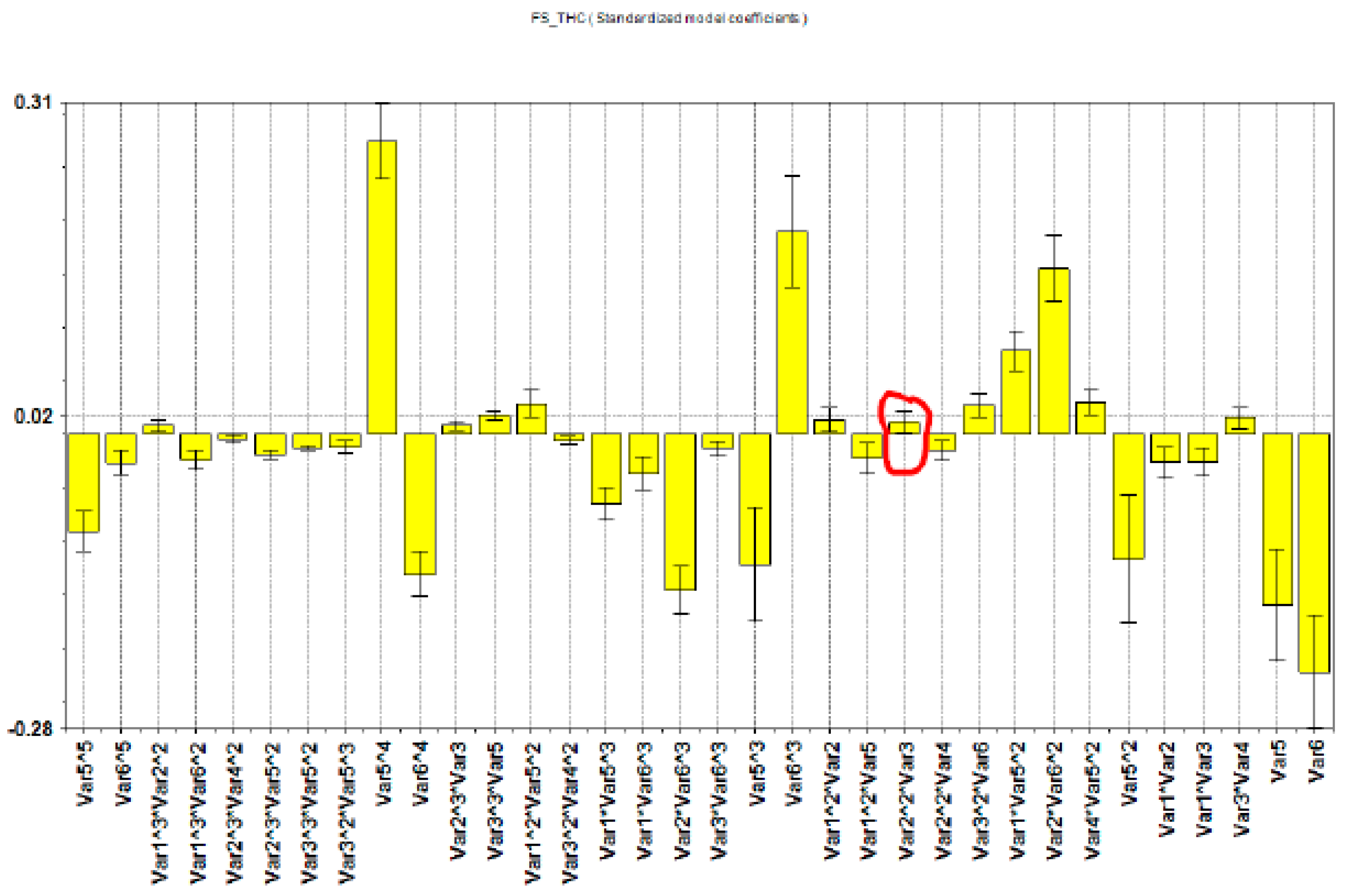
This way, a “grey box” model is obtained, where physical knowledge can be included. The terms within the Equation (10) can be reduced. This means that not all 15 regression coefficients c0, c1, …, c15 will be part of the final model. The model structure graphic in Figure 8 displays standardized HC model coefficients used in the engine model as yellow bars. Error bars of these coefficients describe the 95% confidence intervals. In other words, the graphic displays the influence of each model term on the selected response variable. Terms with a low value but high uncertainty (confidence interval) should be removed to increase the robustness and extrapolation capabilities of the models.
For instance, in Figure 8, the confidence interval for the term circled in red reaches down to near zero. Thus, the coefficient is not significantly different from zero and therefore does not contribute to the quality of the fit and it might even cause spurious behavior in extrapolation, therefore it should be removed.
2.4. Real-Time Exhaust After-Treatment Model
The EAS model has been created independently from the engine model. Finally, a unique model has been created that imports both the engine and EAS models as subsystems linked together. This methodology guarantees high flexibility so that each EAS model could be used for different engine models, maintaining its independence and avoiding useless proliferation. The EAS model is able to simulate the different after-treatment components such as DOC and DPF. Several parameters define the modules: geometry, Platinum Group Metal (PGM) loading, porosity, aging by which heat capacity and pressure losses are calculated. As the chemical reactions that happen in the after-treatment are strongly dependent on the concentration and they change continuously along the flow direction, the mean value is no more effective for this model, while a 1D model is more reliable.
The EAS system of the KDI1903TCR is composed of a DOC and cDPF. Exhaust gas composition and temperature are tracked upstream and downstream of the two catalysts (Figure 9). In order to calibrate the DOC and cDPF models, the following measurements have been performed at the synthetic gas bench (SGB):
- DOC: Light off temperature test (Oxidation of CO, HC and NO)
- DPF: Light off temperature test (Oxidation of CO, HC and NO)
The characteristic time of the EAS model is higher than the engine model so a different and, as mentioned, separate model has been created with a different time-step (1 ms for engine and 100 ms for after-treatment system) and then coupled with the engine model. The EAS is modelled as a sequence of after-treatment component sub-models (e.g., pipes, catalysts and filters). Pipes, catalysts and filters are modeled as systems with one-dimensional (1-D) discretization along the flow direction. Therefore, every system state is calculated and internally cell-wise stored. The aforementioned states include the exhaust gas and the component material temperatures, the gaseous species concentration in the exhausts, the soot loading within the filters and the storage level of absorbed or otherwise non-moving species.
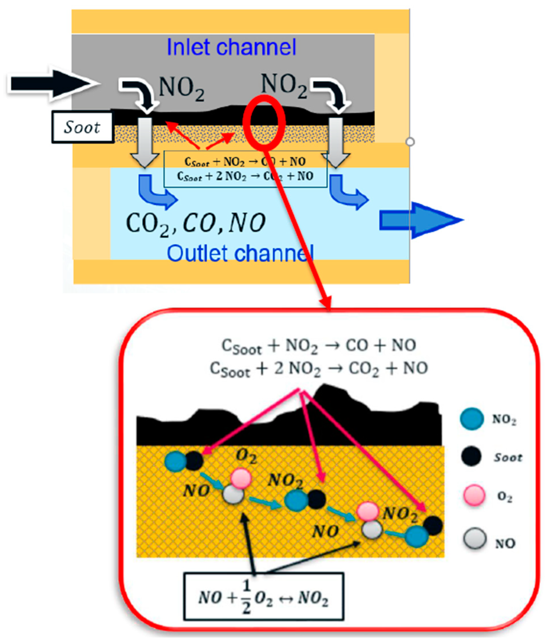
The models for material and gas temperatures contain the heat conduction in the direction of the gas flow in the material and the convective heat transport by the exhaust gas mass flow. Heat exchange between material and gas is evaluated based on Nusselt correlations, whereas heat transfer to the environment considers radiation and convection. Catalyst reactions are modelled based on extended Arrhenius equations and calculated cell-wise. The extensions include inhibition terms and other cross sensitivities. Particulate filter elements (DPF) model individually the exhaust gas flow in inlet and outlet channels. These flow models are connected by a wall-flow model. Mass flow distribution along the channel is used to estimate the amount of soot deposited in the filter. This is calculated depending on soot loading in the individual cell, temperature distribution and pressure loss. In addition, the wall-flow model includes the reaction of deposited soot with oxygen O2 and nitrogen dioxide (NO2), based on an Arrhenius approach. These reactions are paired with the catalytic reaction modelled in the catalyst models (DOC reactions in the cDPF) [41].
2.4.1. Diesel Oxidation Catalyst Model
In this subsection, the methodology for calibrating the global kinetic DOC model is presented. An experimental campaign has been carried out on a reactor-scale sample on an SGB to fully characterize the after-treatment element. These measurements were used to calibrate the global kinetic model.
The experimental activity has been carried out using SGB tests with controlled species concentrations, mass flowrate and inlet temperature by dosing specific species in the inlet batch to minimize the interaction of each reaction on the others and thus facilitating the kinetic model calibration. An isothermal furnace was used to oven age the DOC sample, at 700 °C for 20 h, in an air mixture containing 12% of water vapor. Table 6 reports the main characteristics of the sample:
Concentrations of species including CO, CO2, O2, C3H6, NO, NO2 were acquired at the outlet of the sample by means of Horiba MEXA motor exhaust gas analyzers and Fourier Transform Infra-red spectroscopy (FTIR). K-type thermocouples with a sensitivity of approximately 41 µV/°C, were used to measure inlet and outlet gas temperatures. The experimental test protocol can be categorized into one main group constituted by light-off tests. They were carried out at different levels of standard space velocity (SV), on a temperature ramp from 373 K to 773 K with a constant rate of 15 K/min. The inlet feed gas composition was changed from single trace species to more complex tests, during which several trace species were included in the inlet gases volume. The standard feed composition contained 7.5% O2, 8.5% H2O, 0% CO2, balanced N2 and the trace species as reported in Table 7.
A global reaction model has been defined for the DOC and it is shown in Table 8. Reaction rates have been considered of first order with respect to each reactant concentration (Cxy) and expressed in an Arrhenius form, as can be seen in Table 8 where “Ei” is the activation energy, “Ai” is the pre-exponent multiplier, “T” the catalyst temperature and “R” the universal gas constant. Finally, inhibition term (I) has been defined as in Equation (11) and included in the reaction rate expressions, to fully model the DOC behavior.
with Arrhenius terms for K2…4. The inhibition term accounts for the negative interaction of different species on the same catalytic surface. Furthermore, the chemical reaction number 3 in Table 8 (NO oxidation reaction) has a parameter called “keq” that is the equilibrium term depending only on the catalyst temperature and given by Equation (12):
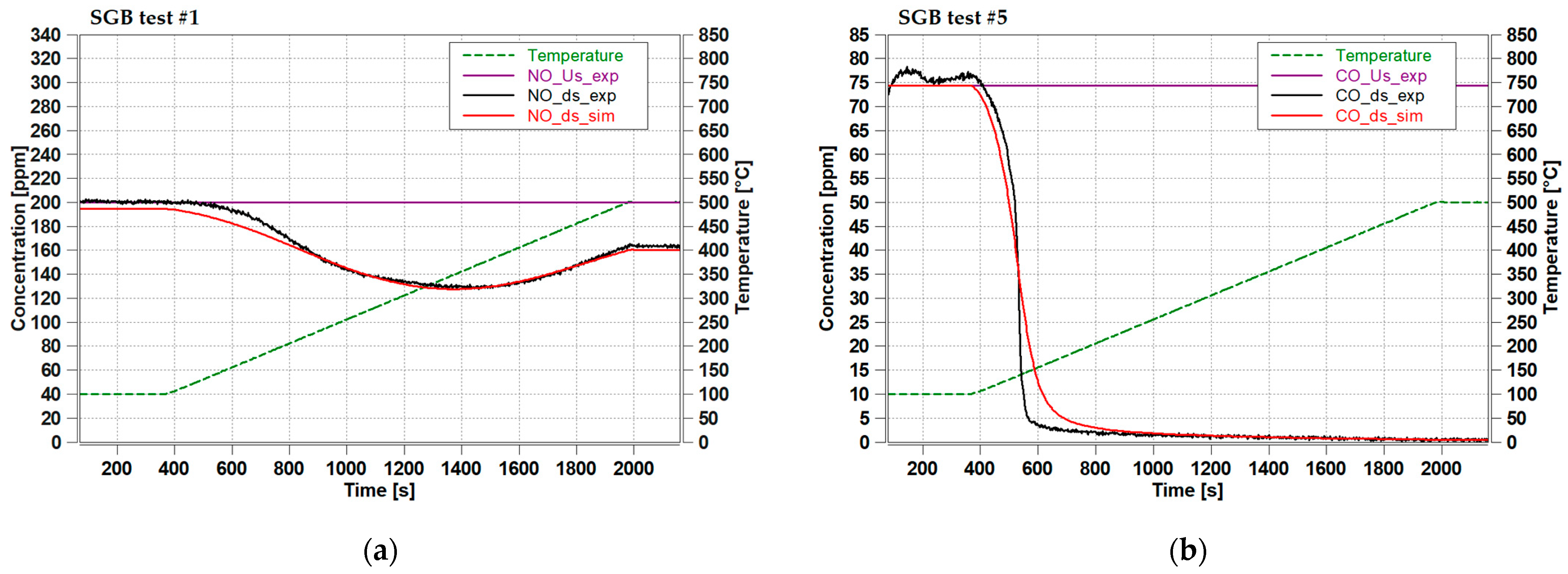
According to the test protocols, the reaction model has been categorized into different steps. In step 1, experimental data of test number 1, 2, 3 and 4 were used to calibrate NO oxidation parameters and inhibition term. This latter was defined after the calibration of oxidation reactions pre-exponent multipliers and activation energies, using data from tests with more than one trace species. In step 2, in addition to inhibition term, CO oxidation parameters were calibrated using test number 5, 6 and 8. In step 3, the calibration of C3H6 oxidation parameters was performed using experimental data of test number 7. To find the correct kinetic parameters, the optimizer embedded in AVL CRUISE M™ has been used to minimize the cumulative absolute error between simulated and measured outlet concentrations of different species. For each reaction defined in Table 8, pre-exponents multipliers and activation energies were tuned and reported in Table 9 while Figure 10a,b show the simulation results of two different SGB tests (#1 and #5) listed in Table 7.
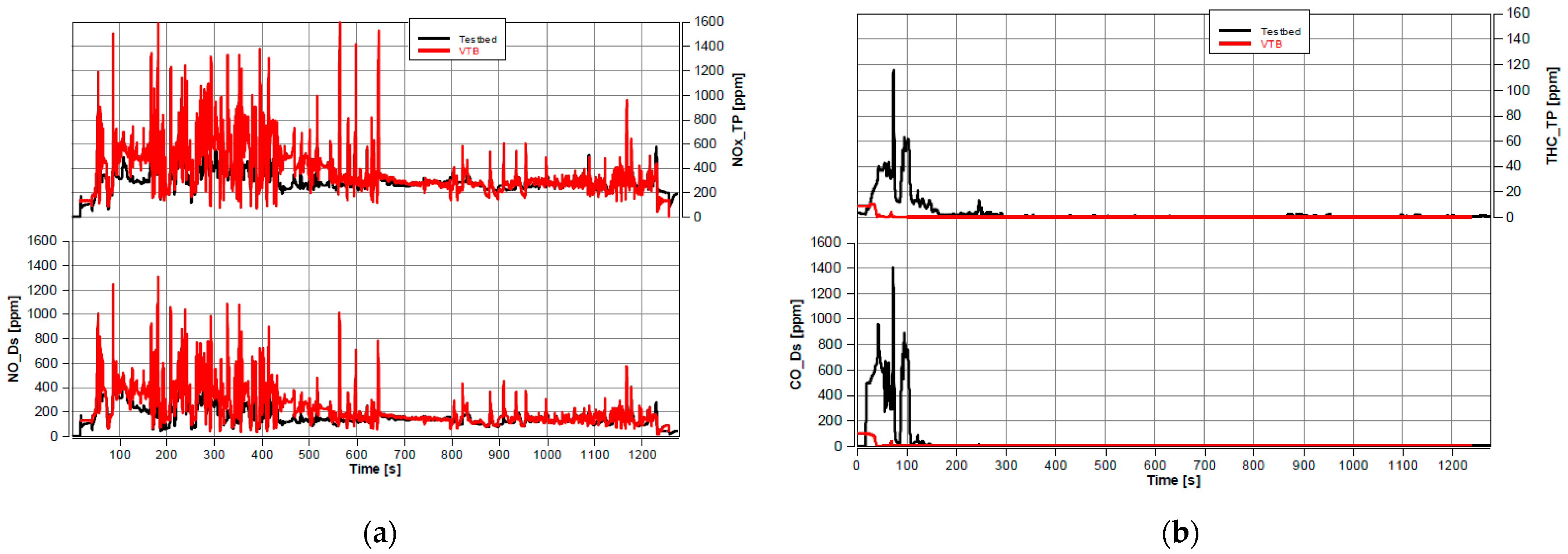
The calibrated kinetic scheme (using SGB data) was finally transferred to the full-size component model (characteristics in Table 6) for the validation over transient cycle data, to evaluate the DOC model accuracy with real exhaust gas conditions as input. The main results are shown in Figure 11.
The sources of different results between reactor-size and full-scale models are the following:
- Non-uniformity of flow and temperature field in full-size component → affecting kinetics.
- The engine exhaust gas includes a mixture of different gas species, especially hydrocarbons.
- Presence of external heat transfer in the full-size component.
- Different aging status of the catalyst components.
2.4.2. Diesel Particulate Filter Model
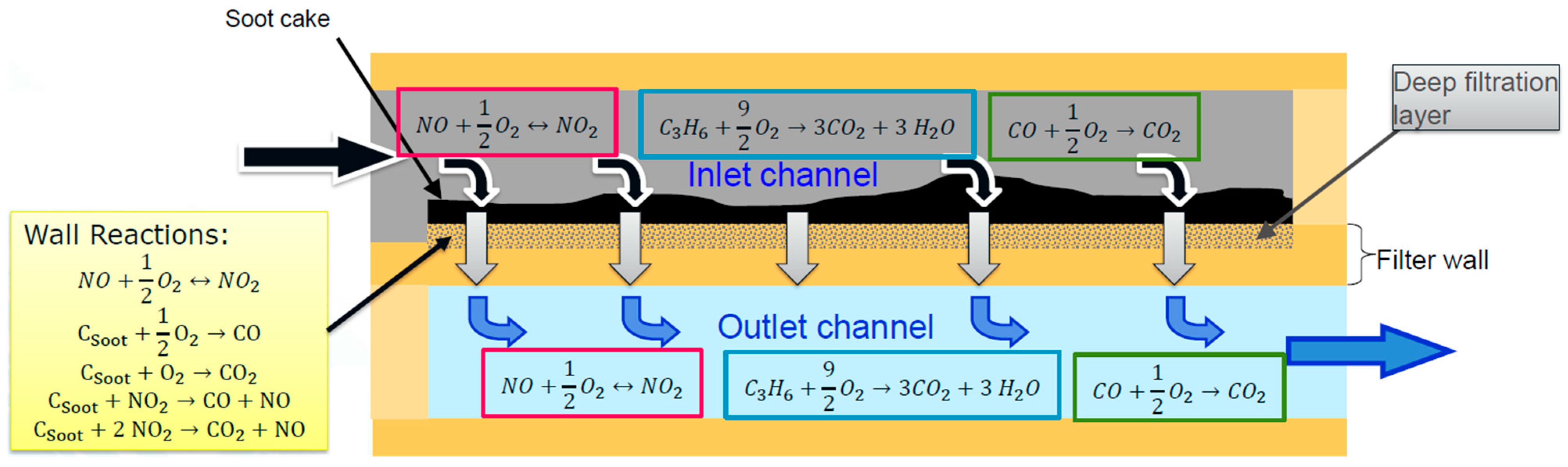
The DPF model is made of two one-dimensional flows, within inlet and outlet channels, coupled with a filtering wall (Figure 12). Inlet and outlet channel models are similar to the DOC model: they contain the three gas reactions for NO, CO and C3H6 as listed in Table 8 for DOC model.
The wall model is the DPF sub-model where soot filtration and oxidation take place. The wall is divided in two physical layers: deep filtration layer and soot cake. In each one of these layers the result of accumulation and oxidation processes are modeled: engine out produced soot is integrated to calculate the accumulation contribution and NO2 and O2 soot oxidation chemical reactions determine the oxidation process. Soot starts to accumulate in the soot cake only when deep filtration layer, which represents the porous part of the wall, is full of soot.
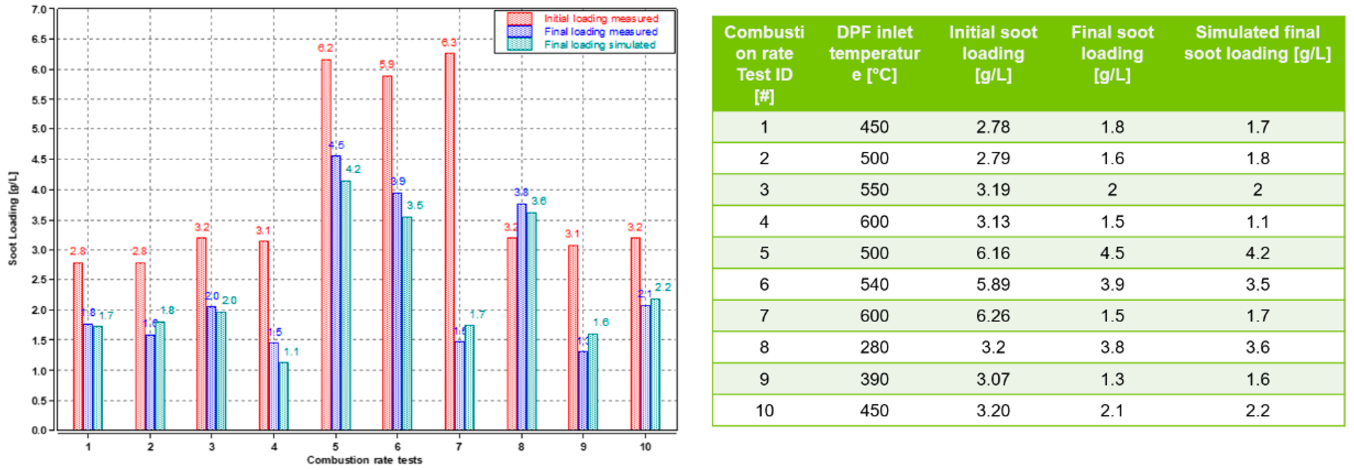
As for the DOC, an experimental campaign has been carried out on a reactor-scale sample on SGB to fully characterize the gas reactions of the filter and the procedure to calibrate the kinetic scheme was exactly the same as the DOC catalyst. After that, different tests at the real engine test bench (named combustion rate experiments) have been performed in order to parametrize the soot oxidation reactions that are the complex part of the DPF model. SGB tests on a reactor-scale sample are indeed not suitable to catch this aspect.
The soot mass in the DPF is reduced by regeneration reactions. These include:
The reaction rates of reactions #1 and #2 detailed in Table 10 contain the distribution factor “fCO” between CO and CO2 that is determined by:
with an exponent qf1 [-] that is dependent on the oxygen concentration and “XO2” that is the oxygen molar fraction. Similarly, in reactions 3 and 4, the distribution factor “gCO” between CO and CO2 is determined by:
In a DPF with PGM coating concurrently to the gas-soot reactions the following NO oxidation reaction takes place:
NO +0.5O2 ↔ NO2
This enables one NO2 molecule entering the wall to oxidize more than one C-atom of the soot layer (Figure 13). The additional NO-oxidation in the wall model leads to the fact that the NO-oxidation is modeled twice:
- as channel reaction (as in the DOC model)
- in the wall
Both NO-oxidation reactions describe the same physical process. The need of wall NO-oxidation reaction comes from details of gas convection and diffusion at the boundary of bulk channel flow and filtration wall not having been modeled explicitly, as a semplification.
2.5. Engine Model Validation on HiL System
Once the plant models are available offline, they are compiled as Functional Mockup Unit (FMU) for the virtual test bed architecture. Subsequently, the main focus becomes the closed loop between models and real hardware (HiL real actuators in Table 2 and engine ECU) to assure the software appropriate functioning within the virtual engine test bed as well as to check the simulation models accuracy before starting the calibration activities that are explained in the following sections.
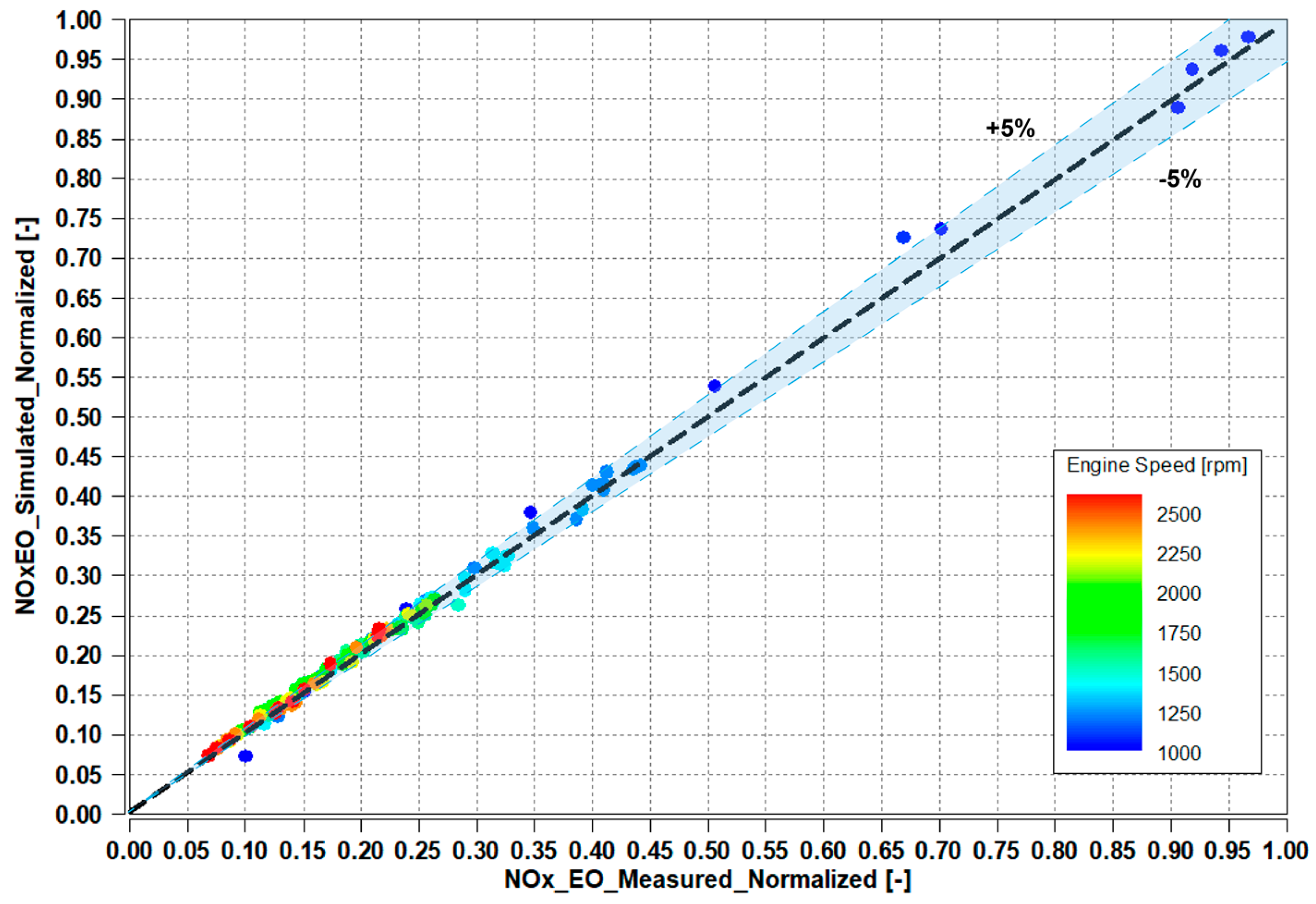
For this research, the engine model was correlated to both steady-state data, acquired in an ICE dynamometer test bench covering the part load and full load operating points across the ICE speed range, and to non-road transient cycle (NRTC), a test cycle required for certification/type approval of Stage V engines. Figure 15 and Figure 16 show a comparison of the NOx and Soot emissions outputs from the engine in the test bed (on the x-axis) and NOx and Soot emissions outputs from the HiL simulation (on y-axis). All the values were normalized with respect to the maximum value of each pollutant reached during the real test. The engine out emissions were used as main parameters for model correlation since they were input to the EAS model. For NOx emissions, the HiL simulation model matched the test bench data within ±5% in the 98% of the tested operating points. This satisfied the correlation criteria for the NOx emission model itself.
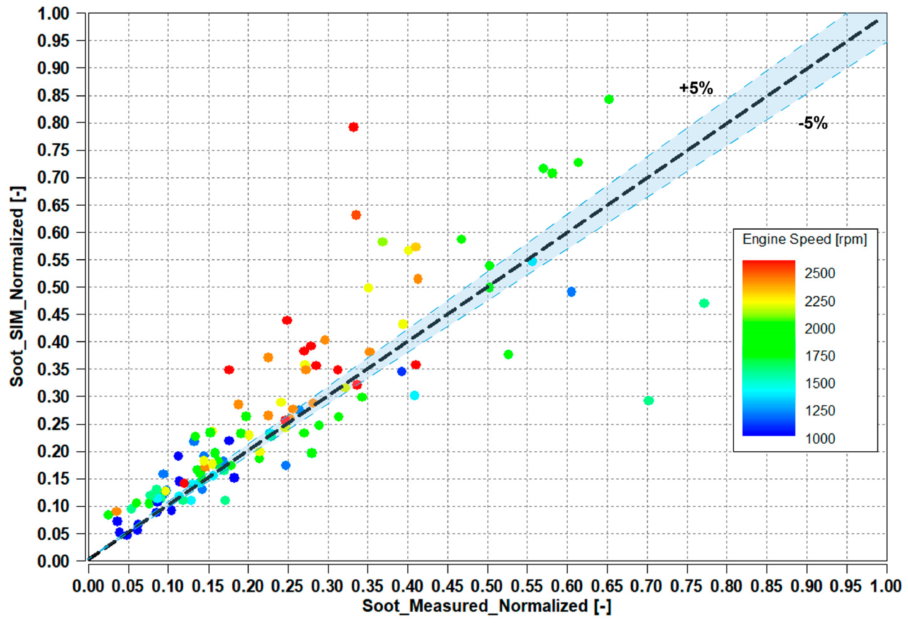
The higher dispersion on Soot (Figure 16), compared to NOx emissions, shows the difficulties in defining an accurate soot model since it depends, more than other emissions, on multiple factors subject to significant engine-to-engine variance. Moreover, local deviations can be explained by highly transient effects that are difficult to replicate on the HiL system.
However, even if the correlation between simulation and test is less satisfactory for soot than it is for other variables, the number of simulated points is in a “safety region” because the simulated soot overall overestimates the real one. Therefore, results have been considered viable.
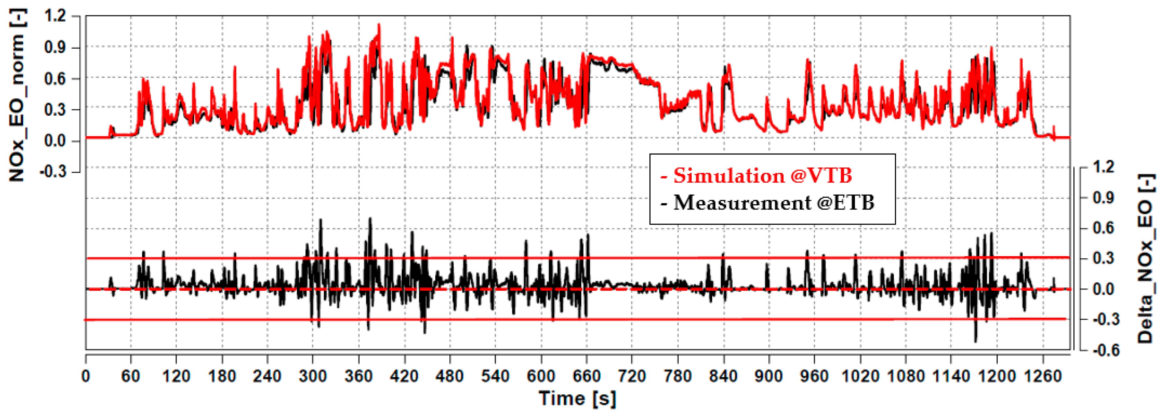
Figure 17 shows a comparison between NOx emissions measured at Engine Out (EO) over the transient cycle (NRTC) and NOx emissions at EO simulated at VTB. The signals are normalized with respect to the maximum NOx experimental value reached during the cycle. In the second row of Figure 17, a difference between simulated NOx trace and measured NOx signal has been reported to better visualize the instantaneous errors.
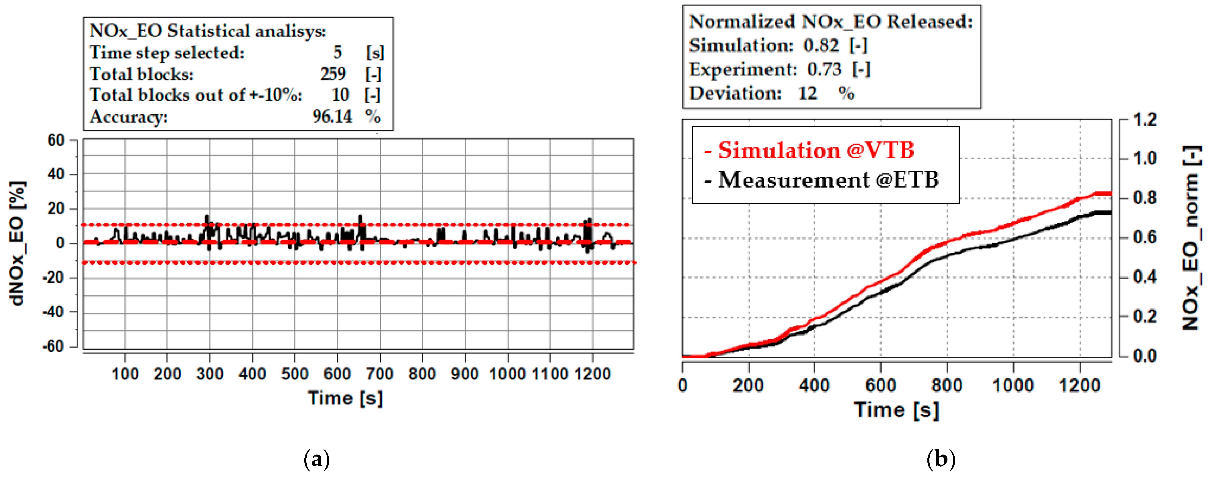
To estimate the accuracy of the engine model running over the NRTC, a statistical analysis has been carried out. In Figure 18a the transient cycle is divided into five seconds blocks. Each block is treated as an independent block and the integration of time-based values is performed. The weighted deviation “dNOx_EO” is calculated taking into account the final accumulated value at the end of the cycle (measurement) and the relative integrator time with respect to the end (Equation (16)):
An indicator of the simulation predictive reliability over the whole cycle can be arrived at counting the quota of blocks within the boundaries of a ±10% error interval (96.14%). Moreover, the accumulated NOx emission simulated over the NRTC (Figure 18b) shows a good agreement with respect accumulated NOx measured at ETB.
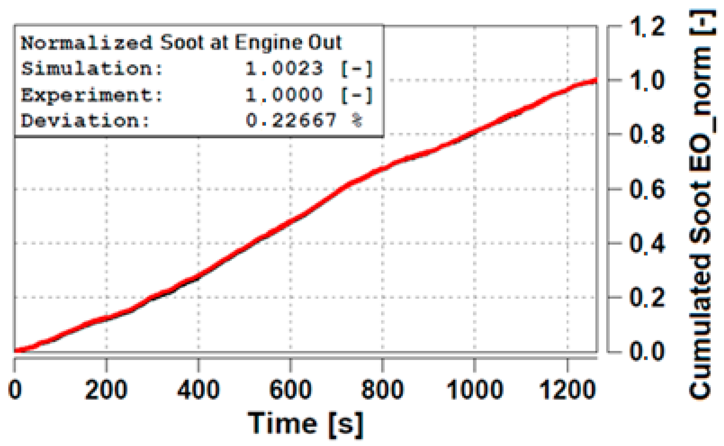
The same statistical analysis has been performed for soot emission. However, for the sake of brevity only the accuracy on the accumulated soot is being reported here. Figure 19 shows the accumulated soot at engine out over an NRTC cycle (normalized with respect to the maximum experimental value reached during the transient cycle), showing a very good agreement between test and simulation, and thereby proving the viability of the HiL system to simulate the soot loading.
Soot loading is certainly one of the most critical variables to be looked in off-road applications because it is directly linked to the cDPF regeneration strategy and so it directly impacts machine productivity. In fact, soot needs to be burned off to regenerate the cDPF, very often while the machine is at a standstill (active regeneration). Thanks to simulation accuracy achievable through the methodology hereby detailed, it is possible to optimize the ECU calibration strategy directly at VTB, so as to minimize the need for active regenerations, limiting downtime and keeping end-user machinery operational and profitable.
Similar validation work was carried out for the EAS model as well.
3. Results and Discussion
3.1. Applications of HiL System for Calibration Activities
After the HiL System validation, the virtual test bed has been widely used to perform the calibration activities. In the following subsections, two different examples are presented. The first one is a calibration activity for machine operation at altitude, finally verified on a vehicle during the fleet validation tests; the second one is a check of a particular duty cycle on a vehicle equipped with KDI 1903 TCR engine: thanks to the presented toolset, analysis of the DPF soot loading could be effectively performed in advance for the real vehicle test.
3.1.1. Altitude Conditions Calibration
During the calibration development, an important milestone is the calibration of non-standard conditions. As standard conditions are referred to sea level and 25 °C, the non-standard conditions refer to altitude, hot and cold conditions. Calibration shall introduce corrections in these particular environments to mitigate the drawbacks. There are engine structural limits that must be respected, e.g., exhaust temperature tends to increase in altitude since AFR (Air to Fuel Ratio) decreases as a consequence of the reduced air density. Moreover, emissions should comply with legislation limits for engine operation at altitudes up to 1680 m above sea level where the engine performance shall be as much as possible similar to those in standard condition.
Generally, this activity would require an extensive test trial with a special emission test bed able to replicate altitude conditions. Thanks to the HiL system, a preliminary calibration could be defined to comply with all the requirements, limiting the utilization of a specific engine test testbed only for a confirmatory final verification. Additionally, some checks can be carried out on the vehicle during specific fleet tests in altitude conditions.
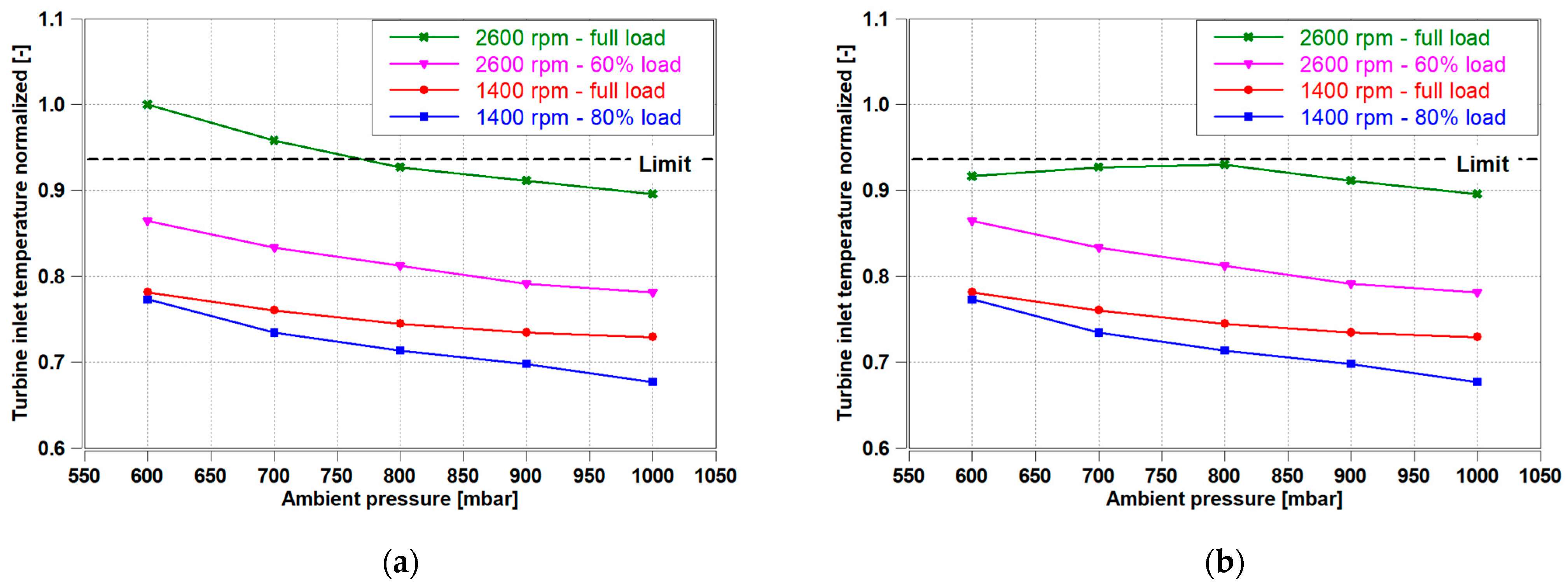
The ambient pressure has been varied at the HiL system in order to calibrate the first ECU dataset for the engine in altitude conditions. At low ambient pressure, the turbine inlet temperature increases together with turbo speed. Both must be kept below the limits to avoid turbocharger failure. The main ICE parameters to be monitored during this test are:
- Turbocharger maximum speed
- Max exhaust port temperature
- Turbine inlet temperature
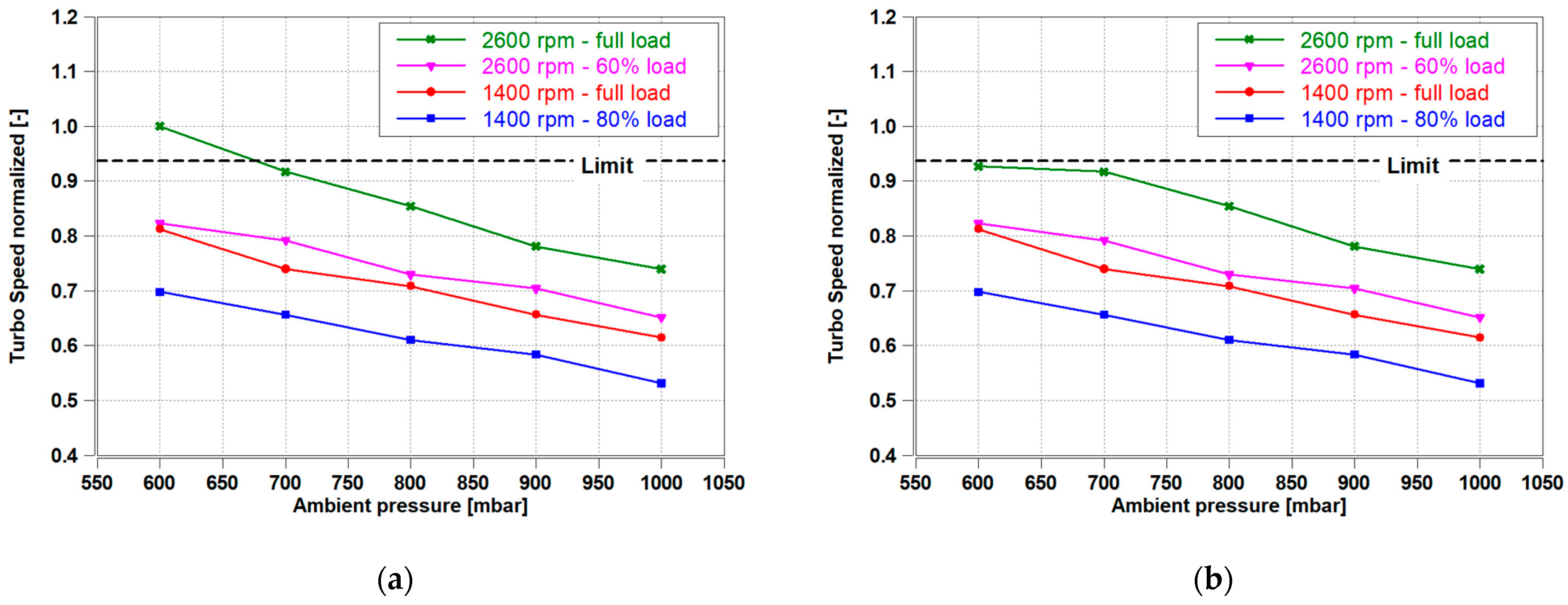
Exhaust temperature increases mainly because of the reduction of air mass flow. Turbocharger speed increases because the turbocharger operating point changes in pressure ratio and mass flow. These two effects (temperature and turbo speed) must be limited to avoid turbocharger damage mainly by applying some fuel limitation depending on ambient pressure. Figure 20a and Figure 21a detail results of the simulation in altitude condition where, below 700 mbar (~3000 m altitude) of ambient pressure, the normalized turbo speed and the normalized turbine inlet temperature for the engine operating point “2600 rpm—full load” are above the structural limits. Figure 20b and Figure 21b display the corresponding behavior after a calibration correction for altitude conditions was defined at VTB.
The engine has been tested at the HiL system at different operating points (the complete full load curve) at different altitudes and the fuel quantity has been reduced until turbo speed and exhaust temperature were below the limit in all the conditions. Thanks to the HiL these calibration adjustments could be provided for at altitudes up to 4000 m (~600 mbar of ambient pressure), a condition which would have been difficult to replicate on a physical test bed or on a vehicle.
Further development involved combustion in extreme conditions, notably focusing on throttle valve and EGR compensation to keep a sufficiently high lambda, fulfilling emissions regulations while delivering optimal performance. Even if above 1680 m emissions are not regulated, it is important to prevent an excessively fast DPF soot loading, which would lead to an increased frequency of active regenerations requests. In altitude, air mass flow is reduced, leading lambda to decrease and exhaust temperature to increase. If these trends were left unchecked, emissions would show an increase in soot and a reduction of NOx. As a countermeasure, the intake throttle valve was opened and EGR was progressively closed.
This activity enabled the definition of calibrations for altitude conditions, compensating the atmospheric pressure reduction, in order to respect component structural limits by appropriate control of actuators (EGR and Throttle Valves). Similar results could be also derived from 1D simulation, but thanks to the HiL System the process has become much more streamlined and less error-prone, as the task can be independently performed by a calibration engineer who directly defines the labels in the ECU.
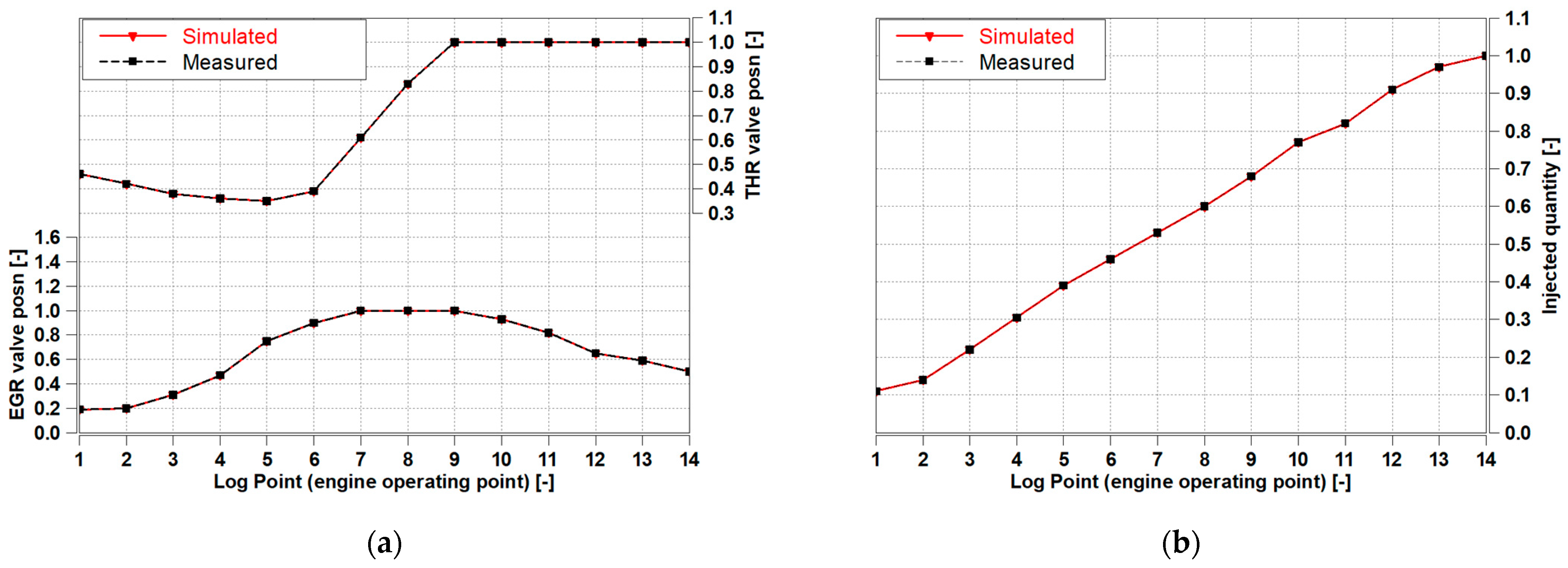
As development progressed, vehicle fleet tests were a useful opportunity to check the results obtained on the HiL System using the vehicle data recording. In the next example, measurements collected on a vehicle in altitude conditions have been compared with HiL simulation. The vehicle was an earthmover, tested at 1680 m over sea level, at the atmospheric pressure of 824 mbar. Some typical engine operating points (named in Figure 22, Figure 23 and Figure 24 “Log point”) have been recorded on the vehicle in altitude and lately have been replicated on the HiL system to check both the ECU outputs that drive the actuators (EGR, throttle valves, fueling) and the main values recorded by engine sensors (turbo speed, boost pressure, intake manifold temperature, exhaust temperatures, NOx).
In Figure 22a,b (normalized with respect to the maximum value reached during the test for each parameter) the inputs for the above-mentioned actuators are shown. The outputs of the ECU are the same on the vehicle and on the HiL System; it is expected but it is an important check and verification that the real altitude condition is well simulated.
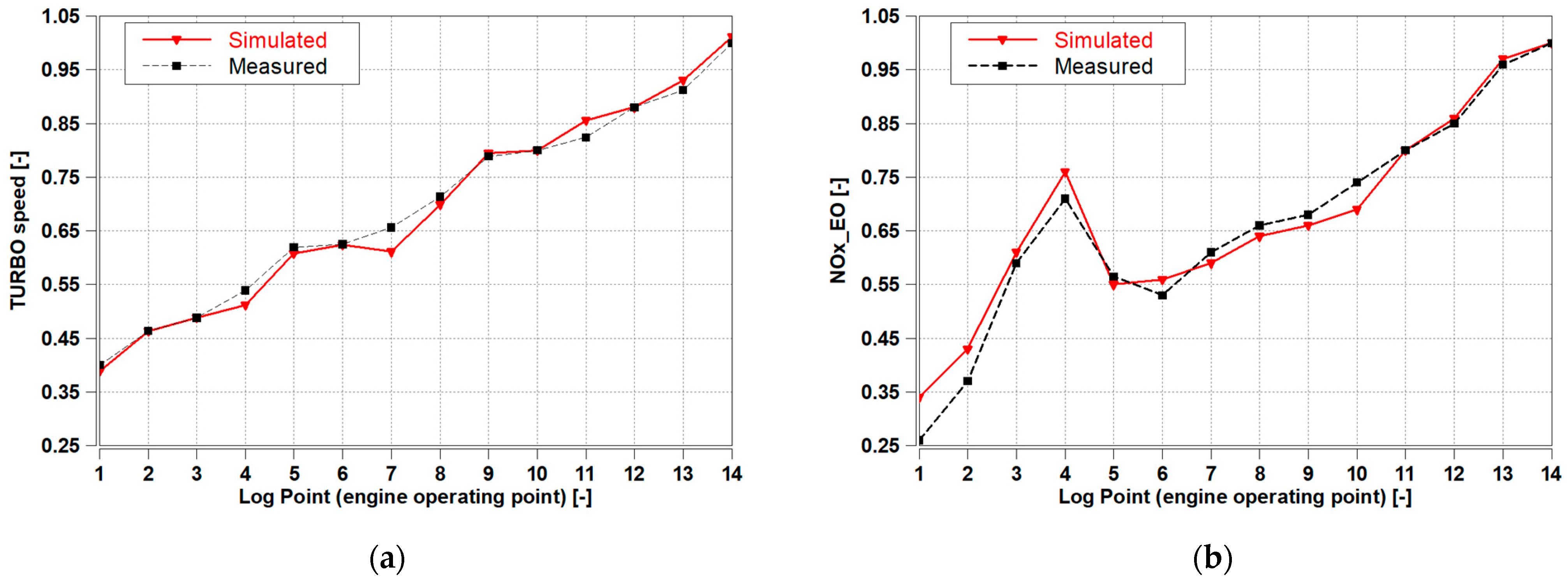
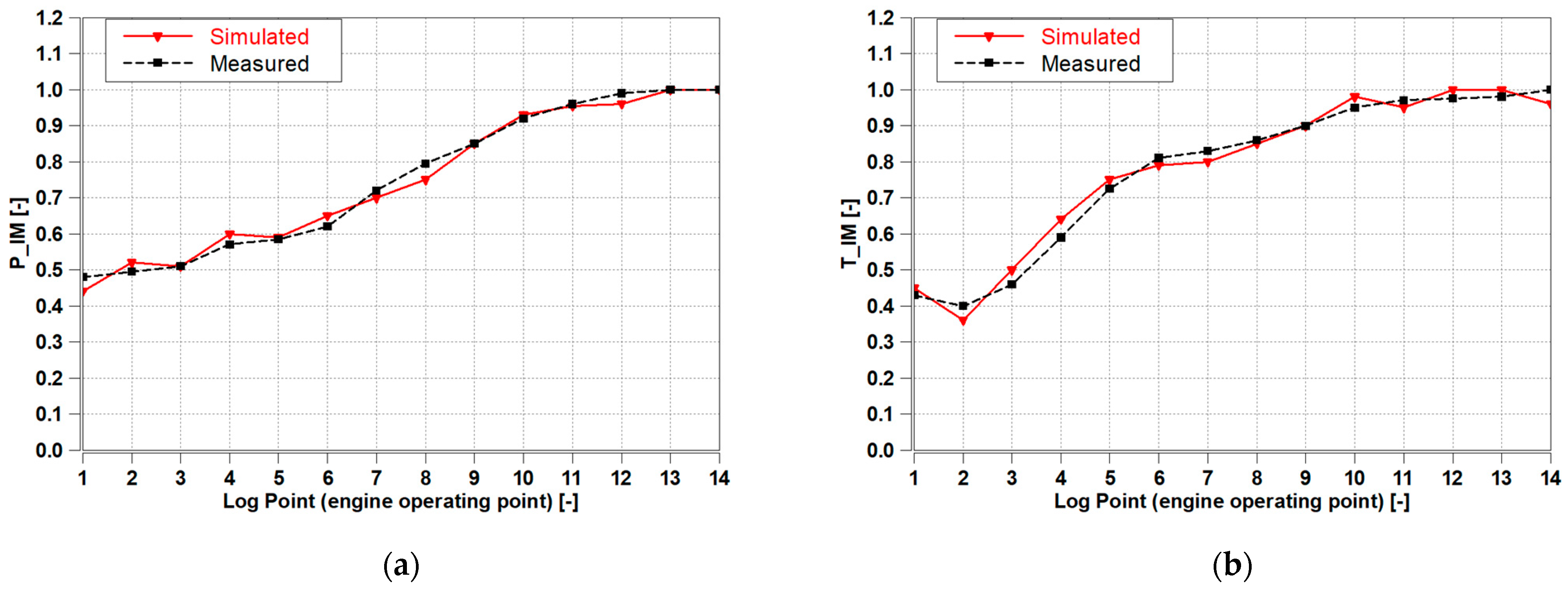
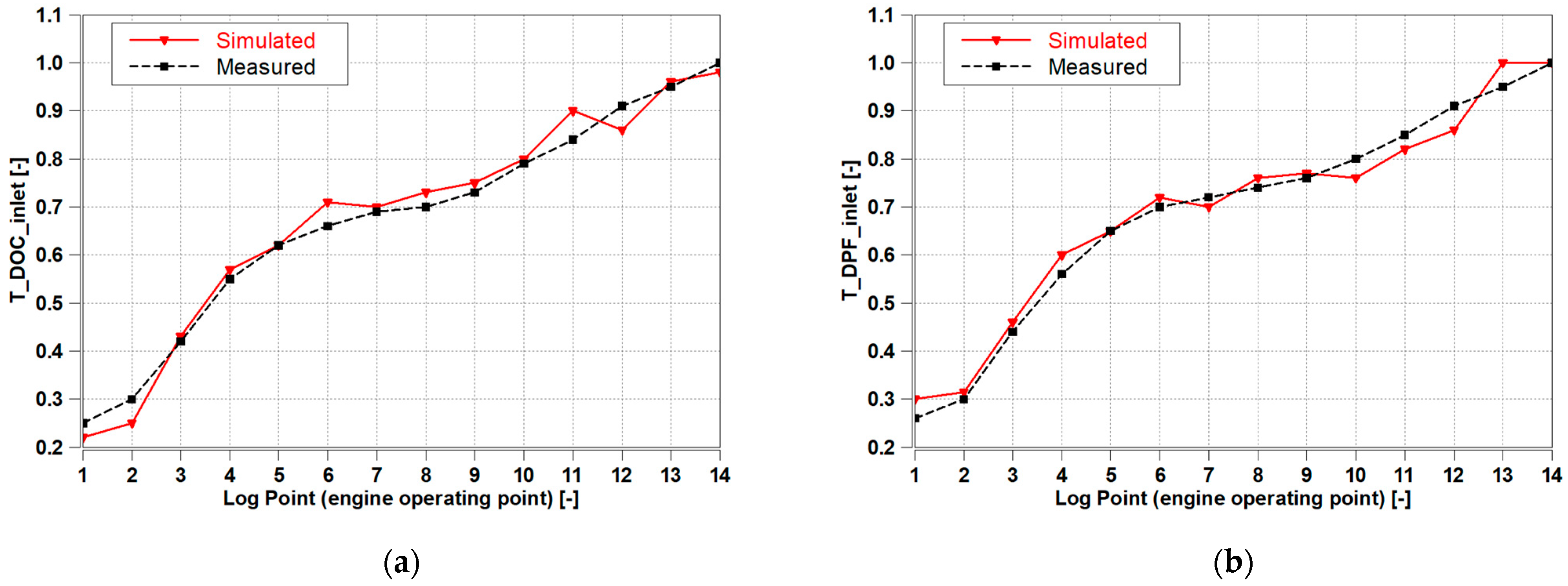
Figure 23, Figure 24 and Figure 25 show normalized data logged from vehicle sensors overlaid on top of data from HiL simulations. The chosen variables, only available on vehicle logs, show a good agreement between engine and simulation with special regard to airflow (turbo speed, pressure and temperature at intake manifold), combustion (NOx, DOC Upstream Temperature) and after-treatment (DOC Downstream Temperature). Figure 23a (normalized with respect to the maximum turbo speed) shows a good match of turbo speed, evidencing accurate Turbocharger modelling. Figure 24a,b intake manifold temperature and pressure show a good correlation between vehicle and simulation.
NOx emissions have been measured using a sensor installed in the exhaust gas flow downstream DPF, that measure NOx concentration at tailpipe; it is an additional sensor added on purpose for this altitude analysis. The good correlation in NOx emissions (Figure 23b) and DOC upstream temperature (Figure 25a) reveals a good matching of the combustion.
The matching in DOC downstream temperature (Figure 25b) suggests simulation of the Oxidation Catalyst has achieved a satisfactory accuracy, with special regard to thermal dynamics, heat exchange properties and exothermic reactions.
Completion of the extreme condition calibration brings the calibration to quite a high maturity level. By tackling these calibration tasks through the HiL platform, development costs and occupation of engine dynamometer resources could be reduced by 20% and 50%, respectively, with respect to a conventional approach.
3.1.2. Soot Loading Model Calibration
DPF system has been widely used today on off-road diesel engines and has been deemed an essential technology in order to meet the Stage V emission limits in terms of particulate matter (PM) and mostly particulate number (PN). PM in exhaust mass flow is made basically of soot coming from the incomplete combustion within the cylinder. The DPF traps these soot particles through different filtration mechanism such as soot-cake filtration and deep-bed filtration. Since the filter surface is coated with PGM to lower the soot ignition temperature, soot particles are also oxidized in the presence of nitrogen dioxide (NO2) in the exhaust when sufficient exhaust temperature is available (passive regeneration). However, once the soot oxidation rate is lower than the soot accumulation rate, the soot accumulation in DPF causes an increase of engine back pressure penalizing the fuel economy. This may even lead to DPF clogging and DPF damage due to uncontrollable thermal regenerations. To avoid these issues, it is necessary to perform a controlled DPF regeneration (active regeneration) through late post injections into the exhaust stream, upstream the DOC to heat up the exhaust gas temperature burning the accumulated soot. Therefore, it is evident how the soot loading amount is a critical parameter for DPF, quiring a dedicated calibration dataset into the ECU.
The KDI1903TCR DPF regeneration strategy is model-based and not time-based so the regeneration interval is managed by a model present in the ECU that estimates the actual soot loading in the DPF. The advantage is that the regeneration is requested only when really needed. As a drawback complex calibration of the soot model becomes necessary in order to adapt to all possible duty cycles and to all possible ambient conditions. An optimal model-driven regeneration interval is a key factor fulfilling customer usability requirements and is therefore, one of the most urgent performance parameters to be evaluated. In the early stages of the development of a new application, a representative duty cycle is generally the only information available to the engine manufacturer. This is enough to run a first soot accumulation test to evaluate the regeneration interval, either virtually within HiL or, with a greater expenditure of time and effort, on the engine test bed.
In the case study shown in this subsection both, virtual and real tests have been performed. The virtual test has been the preliminary one, while the real test has been carried out later to confirm the accuracy of the simulation at VTB.
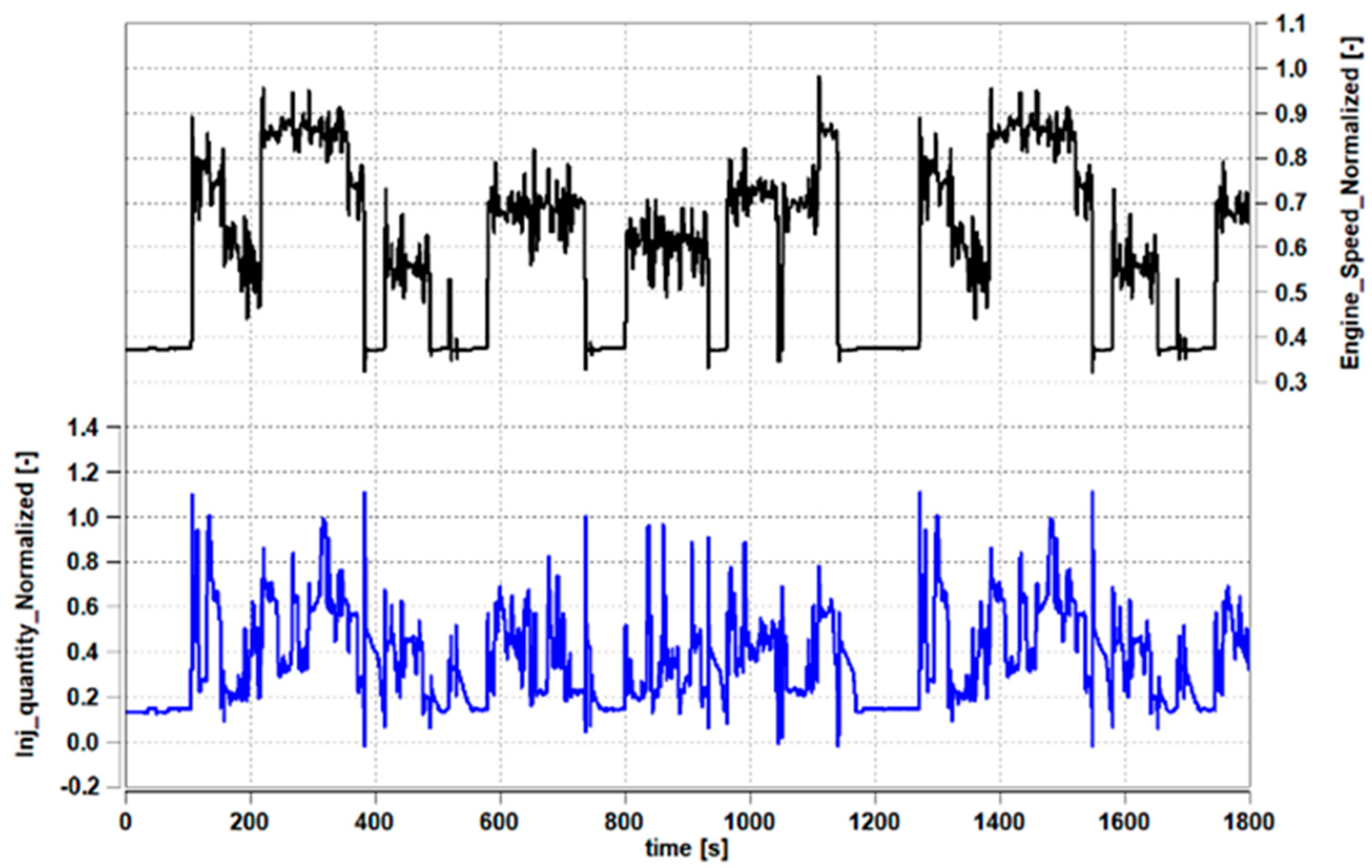
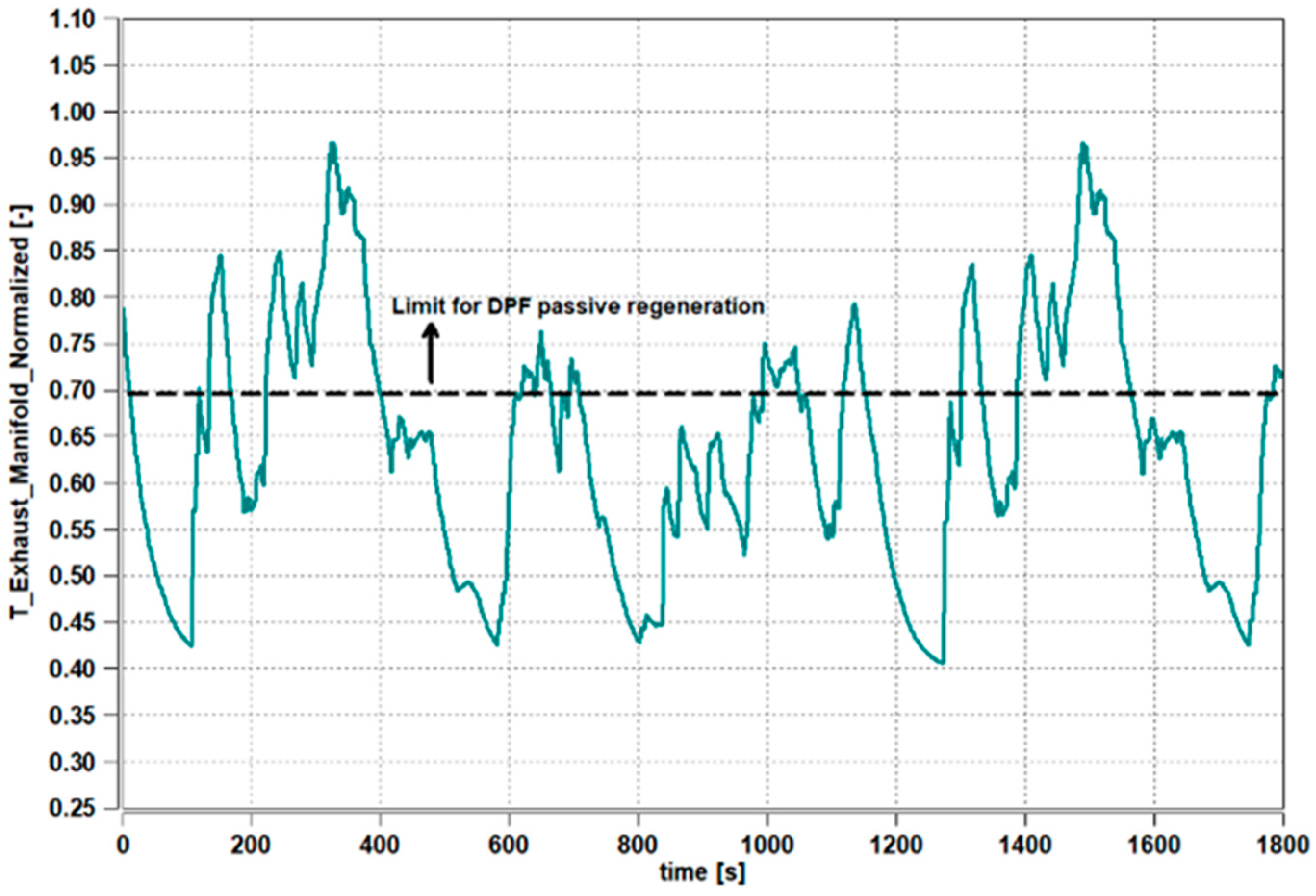
In Figure 26 the normalized duty cycle is shown in terms of engine speed and injected fuel of the specific application that has been simulated on the HiL System and lately on the engine test bed. It is characterized by sudden speed and load transients and some intervals at low idle. It could be classified as a medium-low load cycle. The normalized exhaust temperature (Figure 27) that is an output of the simulation, reflects these transient manoeuvres having some periods above the passive regeneration temperature.
Due to high temperatures, balance between the soot collected in the filter and the soot oxidized with the passive regeneration is to be achieved. It is important to have a confirmation of this trend and verify if an active regeneration is requested. While passive regeneration occurs during the normal cycles with normal combustion, active regeneration requests specific combustion strategies and is generally perceived negatively by customers.
The cycle has been repeated virtually using the HiL System for 70 h and the accumulated soot is shown with a red line in Figure 28. The chart shows that the soot load increases quickly at the beginning, later achieving horizontal asymptote confirming that a balance point is being reached. The same cycle has been run also on an engine test bed, for a confirmation test of the soot loading. This test lasted 30 h (108,000 s), and the accumulated soot has been weighted. The result is shown in Figure 28 with the yellow dot. The difference between simulation and engine testing is 7%, a value that guarantees a good approximation of the phenomenon and could depend on engine-to-engine variance and to different environment conditions: in fact, while on the HiL System the ambient conditions have been set constant, on the engine test stand they vary continuously during testing (e.g., day-night variation).
The result shows that a reliable 0D model of the engine and EAS allows simulating the soot loading behavior for specific duty cycles. This simulation is really powerful as this phenomenon is so complex that experimental results are still widely used for the soot loading evaluation. The advantage of using a virtual calibration approach is the greater flexibility to simulate a wide range of operating conditions, the shorter time to set up the system and no need for maintenance. Additionally, fewer resources (people and material) are required to run the test.
4. Conclusions
The increasing off-road diesel engines multiplicity, merged with a huge number of global emissions regulations and the future establishment of more stringent emission regulations is leading to a substantially growth of development efforts and requirements. Meeting these strict and rigorous demands with traditional methods normally requires the need of supplementary test facilities. Notably, ICE and EAS calibration under extreme environmental conditions such as high altitude and/or low or high temperatures (generally −40 to +50 °C) requires the adoption of costly climatic test cells. Thus, new methodologies are needed to assure reliability, effectiveness and flexibility in order to keep competitive development times and costs in spite of the increasing test needs and complexity.
A virtual calibration approach has been proven to be reliable and efficient in addressing the above-mentioned issues. This method enables to migrate calibration activity from the traditional real test bench to its digital twin, the HiL system or VTB, in which a real ECU and a virtual engine and after-treatment system are running on a virtual test setting.
This solution makes the model-based development and calibration approach more accessible and amenable to being streamlined into an established development process for the calibration engineer. The VTB gives a ready for use solution for virtual calibration.
For the importance of the cited advantages in the engine and EAS development, this activity represents a relevant contribution towards creating accurate models to be applied in optimizing future ICE and EAS operations adopting a model-based approach.
Author Contributions
Conceptualization, A.R.; methodology definition, A.R. and M.L.; software, F.M. and M.L.; validation, A.R. and M.L.; formal analysis, A.R., F.M. and M.L.; investigation, A.R., M.L.; writing—original draft preparation, A.R. and F.M.; writing—review and editing, A.R.; supervision, F.M.; project administration, A.R. and F.M.; funding acquisition, A.R. All authors have read and agreed to the published version of the manuscript.
Funding
This research received no external funding.
Institutional Review Board Statement
Not applicable.
Informed Consent Statement
Not applicable.
Data Availability Statement
No new data were created or analyzed in this study. Data sharing is not applicable to this article.
Conflicts of Interest
The authors declare no conflict of interest.
Abbreviations
| cDPF | Coated Diesel Particulate Filter |
| CPU | Central Processing Unit |
| DI | Direct Injection |
| DOC | Diesel Oxidation Catalyst |
| DPF | Diesel Particulate Filter |
| EAS | Exhaust After-Treatment System |
| ECU | Engine Control Unit |
| EGR | Exhaust Gas Recirculation |
| EO | Engine Out |
| ETB | Engine Test Bed |
| FMU | Functional Mockup Unit |
| FTIR | Fourier Transform Infrared spectroscopy |
| HiL | Hardware In the Loop |
| HTC | Heat Transfer Coefficient |
| HW | Hardware |
| ICE | Internal Combustion Engine |
| KDI | Kohler Direct Injection |
| MFB | Mass Fraction Burned |
| MiL | Model in the Loop |
| NRTC | Non-Road Transient Cycle |
| OEM | Original Equipment Manufacturer |
| PGM | Platinum Group Metals |
| PM | Particulate Matter |
| PN | Particulate Number |
| RMS | Root Mean Squared |
| SiL | Software in the Loop |
| SW | Software |
| VTB | Virtual Test Bench |
| 0D | Zero-Dimensional |
| 1D | One-dimensional |
References
- Onorati, A.; Montenegro, G. 1D and Multi-D Modeling Techniques for IC Engine Simulation; SAE International: Warrendale, PA, USA, 2020. [Google Scholar]
- Khan, D.; Gül, M.Z. Zero-Dimensional Modelling of a Four-Cylinder Turbocharged Diesel Engine with Variable Compression Ratio and Its Effects on Emissions. SN Appl. Sci. 2019, 1, 1162. [Google Scholar] [CrossRef] [Green Version]
- Deng, J.; Stobart, R. BSFC Investigation Using Variable Valve Timing in a Heavy Duty Diesel Engine. SAE Tech. Pap. 2009. [Google Scholar] [CrossRef]
- Galindo, J.; Lujan, J.M.; Climent, H.; Guardiola, C.; Varnier, O. A New Model for Matching Advanced Boosting Systems to Automotive Diesel Engines. SAE Int. J. Engines 2014, 7, 131–144. [Google Scholar] [CrossRef]
- Leach, F.; Ismail, R.; Davy, M.; Weall, A.; Cooper, B. The effect of a stepped lip piston design on performance and emissions from a high-speed diesel engine. Appl. Energy 2018, 215, 679–689. [Google Scholar] [CrossRef]
- Chase, A.; Miwa, J.; Abidin, Z.; Cung, K. Investigation of an Advanced Combustion System for Stoichiometric Diesel to Reduce Soot Emissions; SAE Technical Paper; SAE International: Warrendale, PA, USA, 2019. [Google Scholar] [CrossRef]
- Millo, F.; Boccardo, G.; Piano, A.; Arnone, L.; Manelli, S.; Tutore, G.; Marinoni, A. Numerical Simulation of the Combustion Process of a High EGR, High Injection Pressure, Heavy Duty Diesel Engine; SAE Technical Paper; SAE International: Warrendale, PA, USA, 2017. [Google Scholar] [CrossRef]
- Piano, A.; Millo, F.; Sapio, F.; Pesce, F.C. Multi-Objective Optimization of Fuel Injection Pattern for a Light-Duty Diesel Engine through Numerical Simulation. SAE Int. J. Engines 2018, 11, 1093–1107. [Google Scholar] [CrossRef]
- Millo, F.; Sapio, F.; Piano, A.; Pesce, F.C. Digital Shaping and Optimization of Fuel Injection Pattern for a Common Rail Automotive Diesel Engine through Numerical Simulation; SAE Technical Paper; SAE International: Warrendale, PA, USA, 2017. [Google Scholar] [CrossRef]
- Meda, L.; Shu, Y.; Romzek, M. Heavy Duty Diesel after-Treatment System Analysis Based Design: Fluid, Thermal and Structural Considerations; SAE Technical Paper; SAE International: Warrendale, PA, USA, 2009. [Google Scholar] [CrossRef]
- Diewald, R.; Cartus, T.; Schüßler, M.; Bachler, H. Model Based Calibration Methodology; SAE Technical Paper; SAE International: Warrendale, PA, USA, 2009. [Google Scholar] [CrossRef]
- Lee, S.-Y.; Andert, J.; Quérel, C.; Schaub, J.; Kötter, M.; Politsch, D.; Hadj-amor, H. X-in-the-Loop-Basierte Kalibrierung: HiL Simulation Eines Virtuellen Dieselantriebsstrangs. In Simulation und Test 2017; Liebl, J., Beidl, C., Eds.; Springer Fachmedien Wiesbaden: Wiesbaden, Germany, 2018; pp. 53–79. [Google Scholar]
- Trampert, S.; Nijs, M.; Huth, T.; Guse, D. Simulation von Realen Fahrszenarien Am Prüfstand. MTZextra 2017, 22, 12–19. [Google Scholar] [CrossRef]
- Wurzenberger, J.C.; Bardubitzki, S.; Kutschi, S.; Fairbrother, R.; Poetsch, C. Modeling of Catalyzed Particulate Filters—Concept Phase Simulation and Real-Time Plant Modeling on HiL. SAE Int. J. Engines 2016, 9, 1720–1734. [Google Scholar] [CrossRef]
- Patil, K.; Molla, S.K.; Schulze, T. Hybrid Vehicle Model Development Using ASM-AMESim-Simscape Co-Simulation for Real-Time HIL Applications; SAE Technical Paper; SAE International: Warrendale, PA, USA, 2012. [Google Scholar] [CrossRef] [Green Version]
- Tietze, N.; Konigorski, U.; Fleck, C.; Nguyen-Tuong, D. Model-Based Calibration of Engine Controller Using Automated Transient Design of Experiment. In 14. Internationales Stuttgarter Symposium; Bargende, M., Reuss, H.-C., Wiedemann, J., Eds.; Springer Fachmedien Wiesbaden: Wiesbaden, Germany, 2014; pp. 1587–1605. [Google Scholar]
- Mizuno, H.; Elbers, R.; Pfeilmaier, P.; Naono, T.; Oyobe, H.; Hanada, H.; Shirota, K.; De Smet, J. Development of Simulation Test Bench (HV-HIL) to Calibrate and Evaluate Hybrid Vehicle Components without Real Engine or Car. In 16. Internationales Stuttgarter Symposium; Bargende, M., Reuss, H.-C., Wiedemann, J., Eds.; Springer Fachmedien Wiesbaden: Wiesbaden, Germany, 2016; pp. 1117–1130. [Google Scholar]
- Blanco-Rodriguez, D.; Vagnoni, G.; Aktas, S.; Schaub, J. Model-Based Tool for the Efficient Calibration of Modern Diesel Powertrains. MTZ Worldw. 2016, 77, 54–59. [Google Scholar] [CrossRef]
- Schäuffele, J.; Zurawka, T. Automotive Software Engineering—Grundlagen, Prozesse, Methoden Und Werkzeuge Effizient Einsetzen (3. Aufl.); Vieweg & Sohn: Wiesbaden, Germany, 2006. [Google Scholar]
- Linssen, R.; Uphaus, F.; Mauss, J. Simulation Vernetzter Steuergeräte Für Die Fahrbarkeitsapplikation. ATZelektronik 2016, 11, 16–21. [Google Scholar] [CrossRef]
- Caraceni, A.; De Cristofaro, F.; Ferrara, F.; Scala, S.; Philipp, O. Benefits of Using a Real-Time Engine Model During Engine ECU Development; SAE Technical Paper; SAE International: Warrendale, PA, USA, 2003. [Google Scholar] [CrossRef]
- Lee, S.; Andert, J.; Neumann, D.; Querel, C.; Scheel, T.; Aktas, S.; Miccio, M.; Schaub, J.; Koetter, M.; Ehrly, M. Hardware-in-the-Loop-Based Virtual Calibration Approach to Meet Real Driving Emissions Requirements. SAE Int. J. Engines 2018, 11, 1479–1504. [Google Scholar] [CrossRef]
- Pfau, R.U.; Schaden, T. Real-Time Simulation of Extended Vehicle Drivetrain Dynamics. In Multibody Dynamics: Computational Methods and Applications; Arczewski, K., Blajer, W., Fraczek, J., Wojtyra, M., Eds.; Springer: Dordrecht, The Netherlands, 2011; pp. 195–214. ISBN 978-90-481-9971-6. [Google Scholar]
- Schernus, C.; Lütkemeyer, G.; Winsel, T.; Ayeb, M.; Theuerkauf, H.J.; Pischinger, S. HiL-Calibration of SI Engine Cold Start and Warm-Up Using Neural Real-Time Model; SAE Technical Paper; SAE International: Warrendale, PA, USA, 2004. [Google Scholar] [CrossRef]
- He, Y.; Lin, C.-C. Development and Validation of a Mean Value Engine Model for Integrated Engine and Control System Simulation; SAE Technical Paper; SAE International: Warrendale, PA, USA, 2007. [Google Scholar] [CrossRef] [Green Version]
- Canova, M.; Fiorani, P.; Gambarotta, A. A Real-Time Model of a Small Turbocharged Multijet Diesel Engine: Application and Validation; SAE Technical Paper; SAE International: Warrendale, PA, USA, 2005. [Google Scholar] [CrossRef]
- Katrašnik, T.; Heinzle, R.; Wurzenberger, J.C. Detailed Engine and Vehicle Plant Model to Support ECU Calibration. In Proceedings of the Powertrain Modeling Conference, Bradford, UK, 4–6 September 2012. [Google Scholar]
- Guzzella, L.; Onder, C. Introduction to Modeling and Control of Internal Combustion Engine Systems; Springer Science & Business Media: Berlin/Heidelberg, Germany, 2009; ISBN 3-642-10775-3. [Google Scholar]
- Fuchs, G.; Steindl, A.; Jakubek, S. Local Jacobian Based Galerkin Order Reduction for the Approximation of Large-Scale Nonlinear 664 Dynamical Systems. Int. J. Math. Model. Methods Appl. Sci. 2011, 5, 567–576. [Google Scholar]
- Müller, M.; Hendricks, E.; Chevalier, A. On the Validity of Mean Value Engine Models During Transient Operation; SAE Technical Paper; SAE International: Warrendale, PA, USA, 2000. [Google Scholar] [CrossRef]
- Pischinger, S.; Schernus, C.; Winsel, T.; Ayeb, M.; Wilhelm, C.; Theuerkauf, H.J.; Woermann, R. HiL-Based ECU-Calibration of SI Engine with Advanced Camshaft Variability; SAE Technical Paper; SAE International: Warrendale, PA, USA, 2006. [Google Scholar] [CrossRef]
- Katrašnik, T. Transient Momentum Balance—A Method for Improving the Performance of Mean-Value Engine Plant Models. Energies 2013, 6, 2892–2926. [Google Scholar] [CrossRef] [Green Version]
- Isermann, R. Engine Modeling and Control: Modeling and Electronic Management of Internal Combustion Engines; Springer: Berlin/Heidelberg, Germany, 2014; ISBN 978-3-642-39933-6. [Google Scholar]
- Lee, S.; Andert, J.; Pischinger, S.; Ehrly, M.; Schaub, J.; Koetter, M.; Ayhan, A.S. Scalable Mean Value Modeling for Real-Time Engine Simulations with Improved Consistency and Adaptability; SAE Technical Paper; SAE International: Warrendale, PA, USA, 2019. [Google Scholar] [CrossRef]
- Stage V Regulation (EU) 2016/1628. Available online: http://data.europa.eu/eli/reg/2016/1628/oj (accessed on 7 September 2021).
- KOHLER KDI 1903 TCR. Available online: https://kohlerpower.com/en/engines/product/kdi1903tcr (accessed on 7 September 2021).
- AVL CRUISETM M v2019 User Manual—Chapter 6.1.7; Hans-List-Platz 1, 8020 Graz, AVL List GmbH, MOBEOTM Cylinder; Mobicom Technologies Pvt Ltd.: Bengaluru, India, 2019.
- Oppenauer, K.; Alberer, D.; del Re, L. Simplified Calculation of Chemical Equilibrium and Thermodynamic Properties for Diesel Combustion. SAE Int. J. Engines 2011, 4, 2257–2277. [Google Scholar] [CrossRef]
- Riccio, A.; Di Iorio, F.; Siccardi, F.; Severi, D.; Lucchetti, G.; Karlon, A.; Valchev, P. Heavy Duty Diesel Engine and EAS Modelling and Validation for a Hardware-in-the-Loop Simulation System; SAE Technical Paper; SAE International: Warrendale, PA, USA, 2019. [Google Scholar] [CrossRef]
- Incropera, F.P. Fundamentals of Heat and Mass Transfer, 7th ed.; John Wiley: Hoboken, NJ, USA, 2011. [Google Scholar]
- Missen, R.W.; Mims, C.A.; Saville, B.A. Introduction to Chemical Reaction Engineering and Kinetics; John Wiley & Sons, Inc.: New York, NY, USA, 1999. [Google Scholar]
Figure 1.
Virtualization process to reduce ICE development cost and timing and to go faster to Start of Production (SOP) stage.
Figure 1.
Virtualization process to reduce ICE development cost and timing and to go faster to Start of Production (SOP) stage.

Figure 2.
Hardware in the Loop Simulator.

Figure 3.
Kohler KDI 1903 engine: experimental setup layout and engine schematic.

Figure 4.
Engine Model sketch in AVL CRUISE™ M environment.

Figure 5.
Parametrization of the flow coefficient of the intake throttle valve.

Figure 6.
Coolant temperature: model description.

Figure 7.
External emission models for CO, THC and Soot.

Figure 8.
HC Model Structure graphic.

Figure 9.
Exhaust after-treatment system of KDI 1903 TCR engine.

Figure 10.
(a) Simulated (red) vs. experimental (black) NOx emission downstream DOC. (b) Simulated (red) vs. experimental (black) HC emission downstream DOC.
Figure 10.
(a) Simulated (red) vs. experimental (black) NOx emission downstream DOC. (b) Simulated (red) vs. experimental (black) HC emission downstream DOC.

Figure 11.
(a) Top: Simulated (red) vs. experimental (black) NOx emission downstream DOC. Bottom: Simulated (red) vs. experimental (black) NO emission downstream DOC. (b) Top: Simulated (red) vs experimental (black) HC emission downstream DOC. Bottom: Simulated (red) vs experimental (black) CO emission downstream DOC.

Figure 12.
DPF model overview.

Figure 13.
DPF—NO2 recycling.

Figure 14.
DPF Combustion rate simulated tests.

Figure 15.
Measured (x-axis) vs. Simulated (y-axis) NOx emissions at Engine Out (normalized).

Figure 16.
Measured (x-axis) vs. Simulated (y-axis) Soot emission at Engine Out (normalized).

Figure 17.
Top: Simulated (red) vs. experimental (black) NOx Engine Out (normalized). Bottom: Difference between simulated and measured NOx Engine out signals (normalized).
Figure 17.
Top: Simulated (red) vs. experimental (black) NOx Engine Out (normalized). Bottom: Difference between simulated and measured NOx Engine out signals (normalized).

Figure 18.
(a) Statistical analysis of NOx Engine Out simulated at VTB to determine the model accuracy over the NRTC; (b) Simulated (red) vs experimental (black) of cumulated NOx engine Out emission normalized with respect reference value.
Figure 18.
(a) Statistical analysis of NOx Engine Out simulated at VTB to determine the model accuracy over the NRTC; (b) Simulated (red) vs experimental (black) of cumulated NOx engine Out emission normalized with respect reference value.

Figure 19.
Simulated (red) vs. Measured (black) cumulated soot over NRTC Cycle (normalized).

Figure 20.
(a) Turbo speed w/o Altitude Calibration normalized with respect to the maximum value reached in the test; (b) Turbo speed w/ Altitude Calibration normalized with respect to the maximum value reached in the test w/o altitude calibration.
Figure 20.
(a) Turbo speed w/o Altitude Calibration normalized with respect to the maximum value reached in the test; (b) Turbo speed w/ Altitude Calibration normalized with respect to the maximum value reached in the test w/o altitude calibration.

Figure 21.
(a) Turbine inlet temperature w/o Altitude Calibration normalized with respect to the maximum value reached in the test; (b) Turbine inlet temperature w/ Altitude Calibration normalized with respect to the maximum value reached in the test w/o altitude calibration.
Figure 21.
(a) Turbine inlet temperature w/o Altitude Calibration normalized with respect to the maximum value reached in the test; (b) Turbine inlet temperature w/ Altitude Calibration normalized with respect to the maximum value reached in the test w/o altitude calibration.

Figure 22.
(a) Simulated (red) vs measured (black) Intake throttle valve (top) and EGR valve (bottom) positions (normalized with respect to the maximum value reached in the test); (b) Simulated (red) vs measured (black) fuel injection (normalized with respect to the maximum value reached in the test).

Figure 23.
(a) Simulated (red) vs. measured (black) turbocharger speed (normalized with respect to the maximum value reached in the test); (b) Simulated (red) vs. measured (black) NOx engine out emission (normalized with respect to the maximum value reached in the test).
Figure 23.
(a) Simulated (red) vs. measured (black) turbocharger speed (normalized with respect to the maximum value reached in the test); (b) Simulated (red) vs. measured (black) NOx engine out emission (normalized with respect to the maximum value reached in the test).

Figure 24.
(a) Simulated (red) vs. measured (black) intake manifold pressure (normalized with respect to maximum value reached in the test); (b) Simulated (red) vs. measured (black) intake manifold temperature (normalized with respect to maximum value reached in the test).
Figure 24.
(a) Simulated (red) vs. measured (black) intake manifold pressure (normalized with respect to maximum value reached in the test); (b) Simulated (red) vs. measured (black) intake manifold temperature (normalized with respect to maximum value reached in the test).

Figure 25.
(a) Simulated (red) vs measured (black) DOC inlet temperature (normalized with respect to the maximum value reached in the test); (b) Simulated (red) vs measured (black) DPF inlet temperature (normalized with respect to the maximum value reached in the test).
Figure 25.
(a) Simulated (red) vs measured (black) DOC inlet temperature (normalized with respect to the maximum value reached in the test); (b) Simulated (red) vs measured (black) DPF inlet temperature (normalized with respect to the maximum value reached in the test).

Figure 26.
Top: engine speed (normalized with respect to the maximum value reached in the test) of vehicle duty cycle; Bottom: injected quantity of vehicle duty cycle (normalized with respect to the maximum value reached in the test).
Figure 26.
Top: engine speed (normalized with respect to the maximum value reached in the test) of vehicle duty cycle; Bottom: injected quantity of vehicle duty cycle (normalized with respect to the maximum value reached in the test).

Figure 27.
Exhaust Temperature over the Vehicle Duty Cycle (normalized with respect to the maximum value reached in the test).
Figure 27.
Exhaust Temperature over the Vehicle Duty Cycle (normalized with respect to the maximum value reached in the test).

Figure 28.
Soot Loading comparison between HiL simulation and real engine test bed (normalized with respect to the maximum value reached in the test).
Figure 28.
Soot Loading comparison between HiL simulation and real engine test bed (normalized with respect to the maximum value reached in the test).


Table 1.
Components available as real hardware in the HiL cabinet.
| Intake throttle valve |
| Diesel Common Rail Injectors |
| EGR valve |
| Fuel Pump |
Table 2.
Main features of the test engine “Kohler KDI 1903 TCR”.
| Engine type | DI turbocharged 1.9L diesel engine |
| Emission compliance | China 4, US Tier 4 Final, EU Stage V |
| Engine displacement | 1861 cm3 |
| Bore × Stroke | 88 mm × 102 mm |
| Turbocharger | Single stage turbo and mechanical wastegate |
| Fuel injection system | Common Rail |
| EGR path | High Pressure |
| Aftertreatment system | DOC + cDPF |
| Rated power | 42 kW @ 2600 rpm |
| Rated torque | 225 Nm @ 1500 rpm |
Table 3.
Measurement facility specifications.
| Measurement Equipment | Specification |
|---|---|
| Exhaust gas analyser | AVL AMA i60 SII |
| Smoke meter | AVL 483 micro soot sensor |
| DPF weighing scale | Mettler-Toledo KA32s |
| Air flow rate | AVL FLOWSONIX™ Air |
| Fuel flow rate | AVL FUEL MASS FLOW METER |
| Exhaust gas temperature | Sheathed thermocouples |
Table 4.
Combustion model calibration parameters: optimized values.
| Tuning Parameter | Value |
|---|---|
| PSOIC | 0.11 |
| CDC | 0.05 |
| MFBC | 0.46 |
Table 5.
Optimized values of the NOx model calibration parameters.
| Tuning Parameter | Value |
|---|---|
| NEM | 0.21 |
| NHC | 0.33 |
Table 6.
Characteristics of reactor scale DOC sample and DOC full-size catalyst.
| Characteristic | DOC Sample | DOC Full Size |
|---|---|---|
| Diameter [in] × length [in] | 1 × 3 | 2 × 3 |
| Wall thickness [mil] | 4 | 4 |
| Cell density [cpsi] | 400 | 400 |
| PGM loading [-] | Pt and Pd | Pt and Pd |
| Substrate material [-] | Cordierite | Cordierite |
Table 7.
Light off test (SGB): trace species composition.
| SGB Test ID | CO [ppm] | NO [ppm] | C3H6 [ppm] | SV [1/h] |
|---|---|---|---|---|
| 1 | - | 200 | - | 200,000 |
| 2 | - | 20 | - | 200,000 |
| 3 | - | 200 | - | 100,000 |
| 4 | - | 520 | - | 200,000 |
| 5 | 80 | - | - | 200,000 |
| 6 | 80 | - | 24 | 200,000 |
| 7 | - | - | 24 | 200,000 |
| 8 | 80 | 200 | - | 200,000 |
Table 8.
Reaction model for the DOC component; Ai: pre-exponent multiplier, Ei: activation energy, Cxy: concentration, I: inhibition term.
Table 8.
Reaction model for the DOC component; Ai: pre-exponent multiplier, Ei: activation energy, Cxy: concentration, I: inhibition term.
| # | Site | Reaction | Reaction Rate |
|---|---|---|---|
| 1 | PGM | CO + 0.5O2 → CO2 | A1 ·exp(−E1/RT) · CCO·CO2/I |
| 2 | PGM | C3H6 + 4.5O2 → 3CO2 + 3H2O | A2 ·exp(−E2/RT) · CC3H6·CO2/I |
| 3 | PGM | NO + 0.5O2 ↔ NO2 | A3·exp(−E3/RT) · (CNO·(CO2^0.5)−CNO2/keq)/I |
Table 9.
DOC kinetic model: values of reactions activation energies and pre-exponent multipliers.
| Reaction | Activation Energy Ei | Pre-Exponent Multiplier Ai |
|---|---|---|
| 1 | E1 = 72,383 [J/mol] | A1 = 1.18 × 10¹¹ [-] |
| 2 | E2 = 143,460 [J/mol] | A2 = 1.56 × 10¹⁹ [-] |
| 3 | E3 = 6864 [J/mol] | A3 = 1.12 × 10⁴ [-] |
Table 10.
Soot oxidation reactions.
| # | Reaction | Reaction Rate |
|---|---|---|
| 1 | Csoot + 0.5O2 → CO | R1 = fCO·k1·exp(−E1/RT)·CO2 |
| 2 | Csoot + O2 → CO2 | R2 = (1 − fCO)·k1·exp(−E1/RT)·CO2 |
| 3 | Csoot + NO2 → CO + NO | R3 = gCO·k3·exp(−E3/RT)·CNO2 |
| 4 | Csoot + 2NO2 → CO2 + NO | R4 = (1 − gCO)·k3·exp(−E3/RT)·CNO2 |
Table 11.
Optimized values of the DPF tuning parameters.
| Tuning Parameter | Value |
|---|---|
| E1 | 16,264 [J/mol] |
| k1 | 1.4 × 10⁶ [-] |
| E3 | 12,503 [J/mol] |
| k3 | 1.1 × 10¹¹ [-] |
| fCO | 0.1 [-] |
| gCO | 0.9 [-] |
Publisher’s Note: MDPI stays neutral with regard to jurisdictional claims in published maps and institutional affiliations. |
© 2022 by the authors. Licensee MDPI, Basel, Switzerland. This article is an open access article distributed under the terms and conditions of the Creative Commons Attribution (CC BY) license (https://creativecommons.org/licenses/by/4.0/).
Share and Cite
MDPI and ACS Style
Riccio, A.; Monzani, F.; Landi, M. Towards a Powerful Hardware-in-the-Loop System for Virtual Calibration of an Off-Road Diesel Engine. Energies 2022, 15, 646. https://0-doi-org.brum.beds.ac.uk/10.3390/en15020646
AMA Style
Riccio A, Monzani F, Landi M. Towards a Powerful Hardware-in-the-Loop System for Virtual Calibration of an Off-Road Diesel Engine. Energies. 2022; 15(2):646. https://0-doi-org.brum.beds.ac.uk/10.3390/en15020646
Chicago/Turabian StyleRiccio, Antonio, Filippo Monzani, and Maurizio Landi. 2022. "Towards a Powerful Hardware-in-the-Loop System for Virtual Calibration of an Off-Road Diesel Engine" Energies 15, no. 2: 646. https://0-doi-org.brum.beds.ac.uk/10.3390/en15020646
Note that from the first issue of 2016, this journal uses article numbers instead of page numbers. See further details here.