Design and Implementation of Input AC Filters and Predictive Control for Matrix-Converter Based PMSM Drive Systems

Abstract

Matrix converters have many advantages, including high-efficiency, single-stage AC/AC energy conversion, bidirectional power flow, a near-unity input power factor, sinusoidal three-phase input currents, and sinusoidal three-phase output currents. However, matrix converters have 360 Hz voltage pulsations at the virtual DC-bus, which produce input harmonic currents and output harmonic currents, which cause unsatisfactory responses. To solve the problem of the input harmonic currents, a systematic design of an input three-phase current modulation method and an input three-phase AC filter that uses two different design methods are proposed. In addition, to improve dynamic responses, two predictive speed controllers are investigated and compared, and a predictive current controller is studied to reduce the output harmonic currents. A digital signal processor and an FPGA are used to execute the control algorithms. Several experimental results validate the theoretical analysis and show that the proposed methods effectively improve the power quality of the PMSM drive system and its input power-source quality.

1. Introduction

Matrix converters have simple and compact power circuits, which provide bidirectional power flow, sinusoidal input currents, sinusoidal output currents, a unity input power factor, and regeneration capabilities [1]. Recently, matrix converters have gained a lot of attention from researchers, and several have focused on improving the input currents for matrix converters. For example, Lei et al. proposed a damping control of matrix converter via modifying input reference currents by injecting damping signals. By using this method, the oscillations in input currents could be suppressed directly [2]. Sahoo et al. systematically designed an input filter for matrix converters by using an analytical estimation of root-mean-square current ripples. A step-by-step procedure was shown to determine the inductance parameter and capacitance parameter from the specifications of allowable total harmonic distortion in the input currents and voltages. In addition, a resistance parameter was determined to ensure that the filter had a minimum ohmic loss and a reasonable damping factor [3]. Orser et al. investigated using input filter capacitors as an energy storage device when the matrix converter was ridden through [4]. Dasgupta proposed a filter design for direct matrix converters, which focused on dynamic performance and reliable commutation [5]. Kume et al. studied an integrated filter, which reduced common-mode currents, and provided near sinusoidal output voltages. By using that integrated filter, the traditional R-L-C filter was eliminated [6]. Liu et al. investigated a modeling analysis and parameters design of an LC-filter. Those experimental results showed that the LC-filter-integrated quasi-Z-source network provided the necessary functions. As a result, the traditional input filter was eliminated [7].

In this paper, we propose two different approaches for designing the input R-L-C filter of a matrix converter. First, we use a step-by-step procedure to determine the inductance parameter, capacitance parameter, and resistance parameter. This proposed method has some advantages when it is compared to previous papers [3,4]. In the previously published paper [3], three equations with three coupling coefficients were used. As a result, a numeric solution obtained by using a computer simulation was required. To solve this problem, in this paper, we propose three equations in the first method. Each equation is related to only one or two parameters. As a result, the capacitance parameter, inductance parameter, and resistance can be directly solved by using the three equations and simple algebra. In addition, we use a transfer function to determine the required parameters of the R-L-C filter in the second method. After that, we compare the advantages and disadvantages of these two methods. Finally, experimental results demonstrate the effectiveness of the two different filter designs.

Besides dealing with input harmonic currents, the performance of the motor is important as well. Several researchers have concentrated on modulation methods and controller design of matrix converter-based permanent magnet synchronous motor (PMSM) drive systems. For example, Deng et al. proposed a direct torque control for matrix converter-based PMSM drive systems with minimized common-mode voltages [8]. Zhang et al. proposed a modified PI controller and a proportional resonant (PR) controller for matrix converters and then compared their steady-state tracking performance. However, the output of the matrix converter was connected to a three-phase resistor but not a three-phase AC motor [9]. Mubarok et al. implemented a matrix-converter-based IPMSM position control system, in which a model-free predictive current controller was used [10]. Siami et al. proposed a simplified finite control for matrix converter-based PMSM drive systems. By using that simplified method, the computation of the digital signal processor (DSP) was reduced [11]. Xia et al. investigated direct torque control of matrix converter-based PMSM drives by using duty cycles to reduce 30% of torque pulsations [12]. Khiem et al. proposed improving matrix converter-based PMSM drive systems by using an online detection and fault-tolerant switching strategy [13]. Friedli et al. compared the detailed performance of a three-phase AC-AC matrix converter-based PMM drive system and a DC-link voltage back-to-back converter-based PMSM drive system [14]. Furthermore, Di et al. investigated a novel predictive control method with an optimal switching sequence for a two-stage matrix converter [15]. Li et al. implemented a finite set model predictive control strategy for an indirect matrix converter [16]. Di et al. proposed a continuous control (predictive model control) strategy for an indirect matrix converter [17]. Dendouga designed second-order sliding-mode controllers for a direct matrix converter-based PMSM drive system [18]. Bu et al. designed output filters for a GaN-based matrix converter drive system [19]. Feng et al. investigated an improved model predictive control for matrix converters [20]. Orcioni et al. proposed a driving technique for a direct matrix converter based on a sigma-delta modulation technique [21]. Tuyen et al. implemented the space-vector modulation for an indirect matrix converter [22]. He et al. proposed a step-by-step design for a low-pass input filter for a single-stage converter [23].

However, these previous papers, which focused on matrix converter-based PMSM drive systems, only investigated one-step predictive control [10,11,12,13]. The main reason is that the DSP of a matrix converter-based drive system has to execute a four-step commutation, current-loop control, speed-loop control, and coordinate transformation. To fill this research gap, in our paper, an FPGA is used to execute the four-step commutation. In addition, a DSP is used to execute predictive current-control, one-step predictive speed-control, as well as two-step speed-control. Compared to traditional one-step predictive speed-control, the proposed two-step predictive speed-control provides more flexibility in determining the control input of the PMSM drive system and also has fewer steady-state errors than the one-step predictive control. To the authors’ best knowledge, this comparison of the two methods to design the three-phase input filter of the matrix converter and the comparison of the two-step predictive speed-loop control and one-step predictive speed-loop control for a matrix converter PMSM drive system are original and have not been investigated by previously published papers [1,2,3,4,5,6,7,8,9,10,11,12,13,14,15,16,17,18,19,20,21,22,23]. These two methods and their comparison are the main contributions of this paper.

2. Indirect Matrix-Converter Control

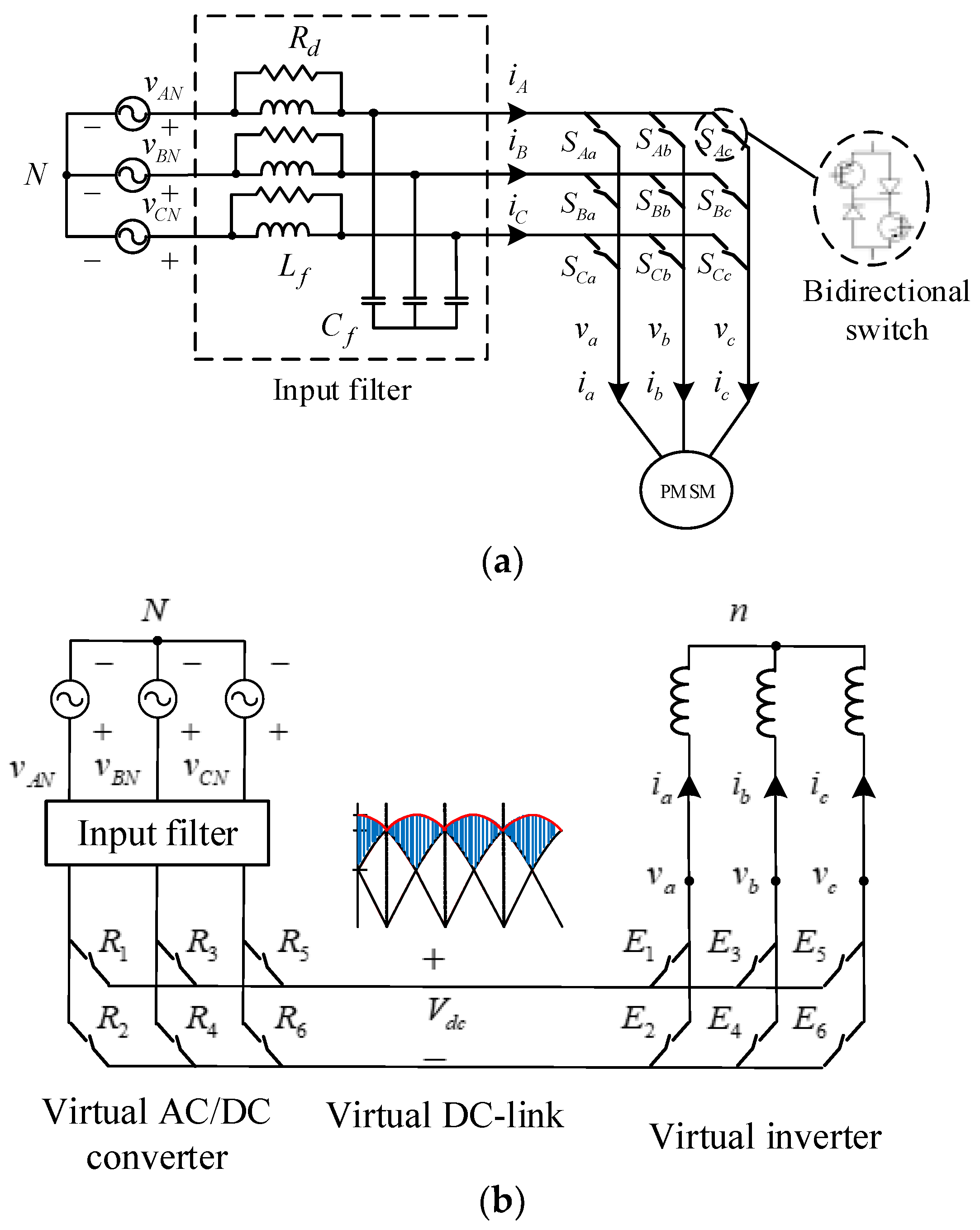
Figure 1a shows the main circuit of the matrix converter. The indirect control of the matrix converter in this paper includes a three-phase input current control and a virtual inverter voltage control, which is shown in Figure 1b. The details are discussed as follows:

The relationship between input voltage and output voltage of the matrix converter in Figure 1a can be shown as the following:

$$\left[\begin{array}{c}{v}_a\\ v_b\\ v_c\end{array}\right]=\left[\begin{array}{ccc}{S}_{Aa}& S_{Ab}& S_{Ac}\\ S_{Ba}& S_{Bb}& S_{Bc}\\ S_{Ca}& S_{Cb}& S_{Cc}\end{array}\right]\left[\begin{array}{c}{V}_{AN}\\ V_{BN}\\ V_{CN}\end{array}\right]$$

(1)

In addition, the switching states of the nine switches in Figure 1a and the equivalent switching states of the relative switches of the virtual AC/DC converter and inverter in Figure 1b are shown as follows:

$$\left[\begin{array}{ccc}{S}_{Aa}& S_{Ab}& S_{Ac}\\ S_{Ba}& S_{Bb}& S_{Bc}\\ S_{Ca}& S_{Cb}& S_{Cc}\end{array}\right]=\left[\begin{array}{cc}{E}_1& E_2\\ E_3& E_4\\ E_5& E_6\end{array}\right]\left[\begin{array}{ccc}{R}_1& R_3& R_5\\ R_2& R_4& R_6\end{array}\right]$$

(2)

2.1. Three-Phase Input Current Control

The desired three-phase input currents are shown as follows:

$$i_A=I_m\cos ({\omega }_{g}t)$$

(3)

$$i_B=I_m\cos ({\omega }_{g}t-\frac{2\pi }{3})$$

(4)

and,

$$i_C=I_m\cos ({\omega }_{g}t+\frac{2\pi }{3})$$

(5)

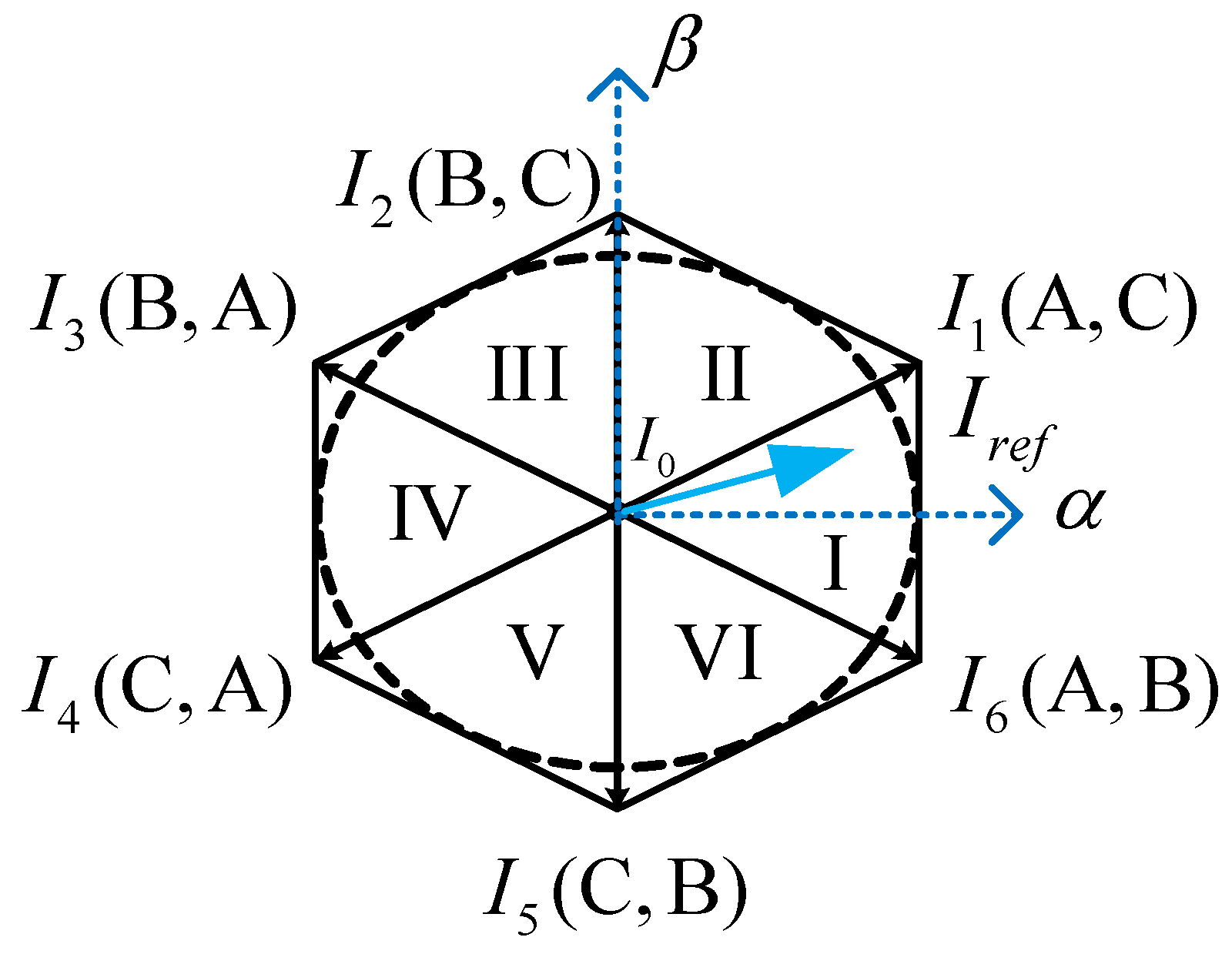
where $i_A$, $i_B$, and $i_C$ are input three-phase currents from the input three-phase voltage source, $I_m$ is the amplitude of the input three-phase currents, and ${\omega }_g{}_{}$ is the angular frequency of the input three-phase voltages or currents. Figure 2 illustrates the space vector of the input current vector, which includes six sections based on the $\alpha$-axis and $\beta$-axis coordinates. First, we assume the input current vector is $I_{ref}$ and is between $I_1$ and $I_6$, which is shown in Figure 2. Then, the input current vector $I_{ref}$ is expressed as follows:

$$\begin{array}{c}{I}_{ref}=\frac{t_{\mu }}{T_s}{I}_1+\frac{t_v}{T_s}{I}_6+\frac{t_0}{T_s}{I}_0\\ =d_{\mu }{I}_1+d_v{I}_6+d_0{I}_0\end{array}$$

(6)

and,

$$d_0=\frac{t_0}{T_s}=1-(d_{\mu }+d_{\nu })$$

(7)

where $I_0$ is the zero current vector; $I_1$ and $I_6$ are the active current vectors; $t_{\mu }$, $t_v$, and $t_0$ are the time intervals of $I_1,$, and $I_0$ individually; and $d_u$, $d_v$, and $d_0$ are the duty cycles of the current vectors $I_1$, $I_6$, and $I_0$ individually. In Figure 2, we can see that when the switches $R_1$ and $R_6$ from Figure 1 are turned on, the switching state of $I_1$(A, C) is created. The other switching states can be expressed in the same way.

Table 1. Relationship between input current vectors and switches.

Input Current Vectors	${\mathit{R}}_1$	${\mathit{R}}_2$	${\mathit{R}}_3$	${\mathit{R}}_4$	${\mathit{R}}_5$	${\mathit{R}}_6$
$I_1$	1	0	0	0	0	1
$I_2$	0	0	1	0	0	1
$I_3$	0	1	1	0	0	0
$I_4$	0	1	0	0	1	0
$I_5$	0	0	0	1	1	0
$I_6$	1	0	0	1	0	0
$I_0$	1	1	0	0	0	0
	0	0	1	1	0	0
	0	0	0	0	1	1

shows the relationship between the input current vectors and the switching states of the virtual AC/DC converter.

2.2. Output Voltage Control of Virtual Inverter

The desired three-phase output voltages are shown as follows:

$$v_a=V_{om}\cos ({\omega }_{o}t)$$

(8)

$$v_b=V_{om}\cos ({\omega }_{o}t-\frac{2\pi }{3})$$

(9)

and

$$v_c=V_{om}\cos ({\omega }_{o}t+\frac{2\pi }{3})$$

(10)

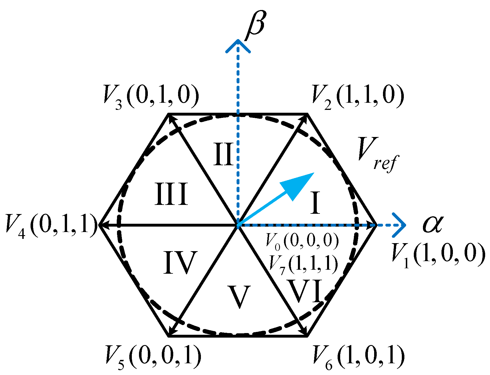
where $v_a$, $v_b$, and $v_c$ are output three-phase voltages, and ${\omega }_o{}_{}$ is the angular frequency of the output three-phase voltages of the virtual inverter. Figure 3 shows the eight space vectors of the output voltage vectors based on the $\alpha$-axis and $\beta$-axis coordinates. In Figure 3, when the output voltage vector is $v_{ref}$ and is located between $V_1$ and $V_2$, then the output voltage vector $v_{ref}$ is shown as follows:

$$\begin{array}{c}{v}_{ref}=\frac{t_1}{T_s}{V}_1+\frac{t_2}{T_s}{V}_2+\frac{t_0}{T_s}{V}_0\\ =d_1{}_{}{V}_1+d_2{}_{}{V}_2+d_0{}_{}{V}_0\end{array}$$

(11)

where $V_0$ is the zero voltage vector; $V_1$ and $V_2$ are the active voltage vectors; $t_1$, $t_2$, and $t_0$ are the time intervals of $V_1$, $V_2$, and $V_0$; and $d_1$, $d_2$, and $d_0$ are the duty cycles of the voltage vectors $V_1$, $V_2$, and $V_0$. The duty cycle of the zero vector is as follows:

$$d_0=\frac{t_0}{T_s}=1-(d_1+d_2)$$

(12)

The switching state of $V_1$ (1, 0, 0) means that when the switch of the virtual inverter $E_1$ turns on, $E_2$ turns off, and when $E_4$ turns on, $E_3$ turns off, and when $E_6$ turns on, $E_5$ turns off, all of which can be seen in Figure 1b. The other switching states can be expressed in the same way.

3. Input Filter Design

A systematic design procedure of the input filter for a matrix converter is described below.

3.1. Method 1

Several papers have investigated the optimal design method of input filters for AC/AC matrix converters [24]. In this paper, by using this systematic design procedure, the parameter ${\lambda }_1$ is used to determine the ratio of the input harmonic currents to the input fundamental currents. Then, the parameter ${\lambda }_2$ is used to determine the ratio of the input harmonic voltages to the input rms voltages. Finally, the ${\lambda }_3$ is used to determine the ratio of the power loss of the R-L-C filter to the rated output power of the matrix converter. The details are discussed as follows.

Step 1: Determine the input current harmonics

In the first step, the input harmonic currents are determined. Then, the input rms value of the fundamental currents of the matrix converter, which also includes $i_A$, $i_B$, and $i_C$, shown in Figure 1a, can be calculated as follows [3]:

$$I_{in1\_RMS}=\frac{3}{2}{m}_I\cdot m_V\cdot I_{o1\_RMS}\cdot \cos {\varphi }_o$$

(13)

where $I_{in1\_RMS}$ is the input rms value of the fundamental currents of the matrix converter, $m_I$ is the modulation index of the input current vectors of the matrix converter, $m_V$ is the voltage modulation index of the virtual inverter, $I_{o1\_RMS}$ is the output rms value of the fundamental current of the matrix converter that includes $i_a$, $i_b$, and $i_c$ shown in Figure 2a, and ${\varphi }_o$ is the phase angle between the output voltages and output currents. In Equation (13), the output rms currents of the fundamental currents of the matrix converter, $I_{o1\_RMS}$, can be expressed as follows:

$$I_{o1\_RMS}=\frac{P_o}{3V_{g\_RMS}\cos {\varphi }_o}$$

(14)

where $P_o$ is the rated output power of the matrix converter and $V_{g\_RMS}$ is the rms value of the fundamental voltages of the input voltage sources. After that, the value of parameter ${\lambda }_1$ can be determined by the designer and is shown as follows:

$${\lambda }_1=\frac{I_{gsw\_RMS}}{I_{in1\_RMS}}$$

(15)

where $I_{gSW\_RMS}$ is the rms value of the switching harmonic currents of the input currents, which includes $i_A$, $i_B$, and $i_C$, and $I_{in1\_RMS}$ is the input rms value of the fundamental currents of the input currents of the matrix converter. From Equation (15), we can obtain:

$$I_{gsw\_RMS}={\lambda }_1{I}_{in1\_RMS}$$

(16)

The ratio of the rms value of the switching harmonic currents of the input currents to the switching harmonic currents of the matrix converter, $I_{insw\_RMS}$, which is related to $I_{in1\_RMS}$, can be determined by the designer. Finally, the relationship between the input harmonic currents and output harmonic currents of the R-L-C filter can be shown as follows [6]:

$$\frac{I_{gSW\_RMS}}{I_{insw\_RMS}}=\frac{1}{\sqrt{1+\frac{{(1 - {\omega }_s{}^2{L}_f{C}_f)}^2 - 1}{(1 + \frac{{\omega }_s{}^2{L}_f{}^2}{R_d{}^2})}}}$$

(17)

where ${\omega }_s$ is the switching frequency, and $L_f$, $C_f$, and $R_d$ are the inductance, capacitance, and resistance of the R-L-C filter. In this paper, the parameters of $L_f$ and $R_d$ are directly obtained from Equations (17) and (21) by using an analytic method without a computer.

Step 2: Determine the input harmonic voltages

In the second step, the input harmonic voltages are determined. First, the ratio between the input harmonic voltages, $V_{in\_ripple}$, and the input rms line voltages, $V_{in\_line\_}{}_{rms}$, is described as follows:

$${\lambda }_2=\frac{V_{in\_ripple}}{V_{in\_line\_}{}_{rms}}$$

(18)

where $V_{in\_ripple}$ is the input harmonic voltages and $V_{in\_line\_}{}_{rms}$ is the input rms line voltages. After that, the capacitance of the input R-L-C filter, $C_f$, is shown as follows [7]:

$$C_f=\frac{I_o}{\pi {\omega }_s{V}_{ripple}}\sin \pi D$$

(19)

where D is the turned-on duty cycles of each switch in the matrix converter.

Step 3: Determine the ratio of the filter power loss to the rated output power

First, the ${\lambda }_3$ is determined by the designer to obtain the ratio of the filter power loss to the rated output power as follows:

$${\lambda }_3=\frac{P_{loss}}{P_o}$$

(20)

After doing some mathematical processes, one can obtain the following equation [6]:

$${\lambda }_3=\frac{I_{in1\_RMS}}{V_{g\_RMS}}(\frac{{\omega }_g{}^2{L}_f{}^2{R}_d}{{\omega }_g{}^2{L}_f{}^2+R_d})$$

(21)

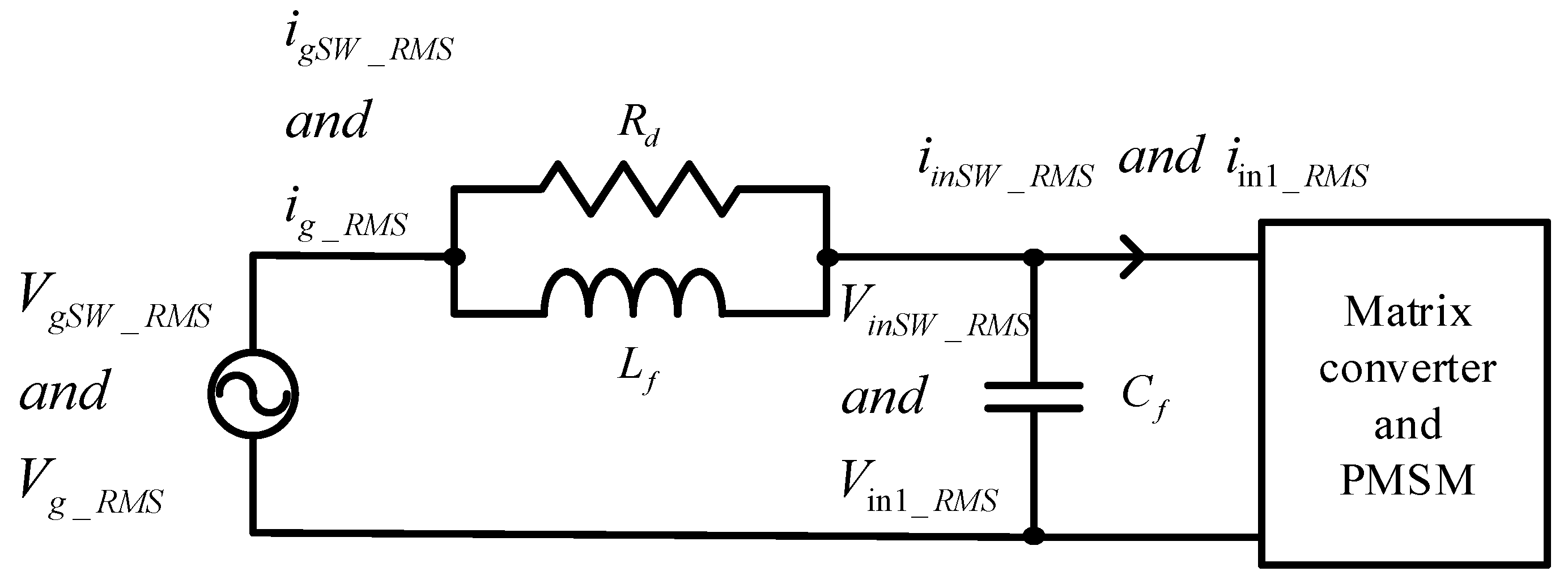
As a result, from Equations (16) and (21), one can obtain the unique solution of the $L_f$, which is the inductance of the R-L-C filter and the $R_d$, which is the resistance of the R-L-C filter. The single-phase equivalent R-L-C filter is shown in Figure 4, which includes the switching RMS voltages, the fundamental RMS voltages, the switching RMS currents, and the fundamental RMS currents.

3.2. Method 2

The second method uses a frequency domain to design the R-L-C filter. The details are described below.

Generally speaking, the R-L-C filter resonant frequency is less than 1/3 of the switching frequency of the matrix converter, and over 20 times greater than the fundamental frequency. The relationship is as follows:

$$20f_g\le f_{res}\le \frac{1}{3}{f}_s$$

(22)

where $f_g$ is the frequency of the input voltage source, $f_{res}$ is the resonant frequency of the filter, and $f_s$ is the switching frequency of the matrix converter. The capacitor $C_f$ of the filter causes a phase shift between the input currents and input voltages. Therefore, the capacitor $C_f$ has to be smaller than the allowed maximum capacitor that causes the allowed maximum phase angle ${\theta }_{\max }$. This relationship is expressed as follows [24]:

$$C_f{<}^{}{C}_f{}^{\max }$$

(23)

and,

$$C_f{}^{\max }=\frac{I_{in1\_RMS}}{V_{g\_RMS}{\omega }_g}\tan {\theta }_{\max }$$

(24)

where $C_f{}^{\max }$ is the allowed maximum capacitor, and ${\theta }_{\max }$ is the allowed maximum phase angle. The resonant frequency is then defined as:

$$f_{res}=\frac{1}{2\pi \sqrt{L_f{C}_f}}$$

(25)

From Equation (25), one can derive the following equation:

$$L_f=\frac{1}{C_f\cdot {\left(2\pi f_{res}\right)}^2}$$

(26)

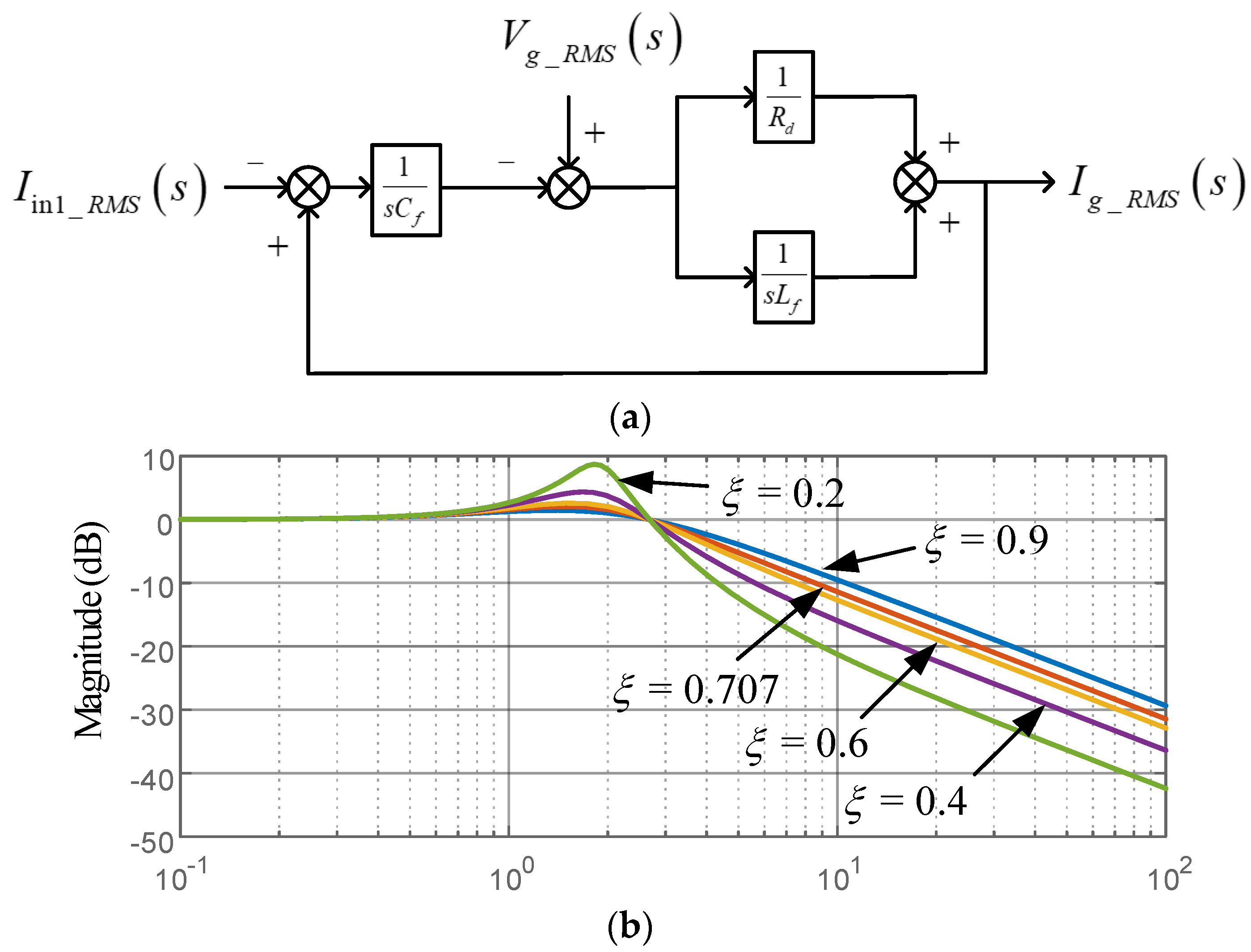
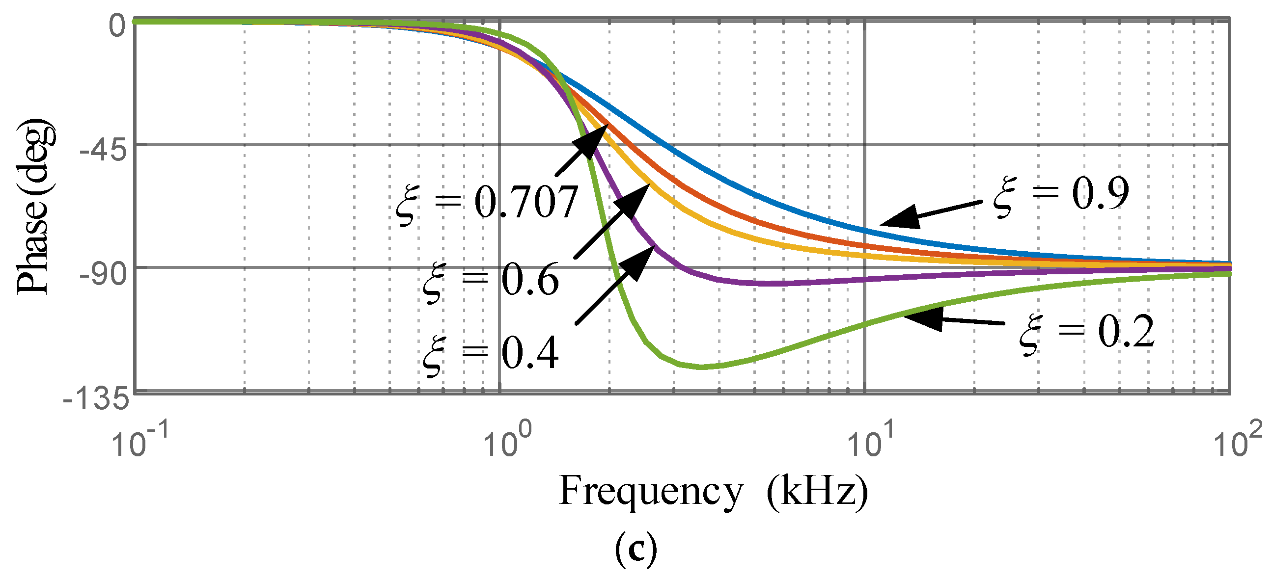
In this paper, the resistance is in parallel with the inductance. The transfer function of the second-order system is shown in Figure 5a and is as follows:

$$\begin{array}{c}\frac{I_{g\_RMS}\left(s\right)}{I_{in1\_RMS}\left(s\right)}=\frac{s\frac{L_f}{R_d}+1}{s^2{L}_f{C}_f+s\frac{L_f}{R_d}+1}\\ =\frac{s\frac{{\omega }_{res}}{Q_{res}}+{\omega }_{res}^2}{s^2+2\xi {\omega }_{res}s+{\omega }_{res}^2}\end{array}$$

(27)

In Equation (27), the related parameters are as follows:

$${\omega }_{res}=\frac{1}{\sqrt{L_f{C}_f}}$$

(28)

$$Q_{res}=R_d\sqrt{\frac{C_f}{L_f}}$$

(29)

and,

$$\xi =\frac{1}{2R_d}\sqrt{\frac{L_f}{C_f}}$$

(30)

where ${\omega }_{res}$ is the resonant frequency in rad/s, $Q_{res}$ is the quality factor, and $\xi$ is the damping ratio. Figure 5b illustrates the relationship of magnitude and frequency in a Bode diagram, and Figure 5c illustrates the relationship of the phase angle and frequency in a Bode diagram for a typical R-L-C filter.

Although the first method requires more complicated computation processes, it obtains the parameters of the R-L-C filter via the THD of the real currents and voltages. The second method quickly determines the parameters of the R-L-C filter; however, it is difficult to estimate the THD of the input current. The major reason is that the second method focuses on frequency-domain responses but not harmonic current or voltage constraints.

4. Predictive Controller Design

4.1. One-Step Predictive Speed Controller Design

The discrete form of the dynamic speed equation for a PMSM is shown as follows [25]:

$${\widehat{\omega }}_m(k+1)=e^{-\frac{B_m{T}_s}{J_m}}{\omega }_m(k) + \frac{1}{B_m}(1-e^{-\frac{B_m{T}_s}{J_m}})T_e(k)$$

(31)

where ${\widehat{\omega }}_m(k+1)$ is the predictive speed at the $\left(k+1\right)$th sampling interval, $T_s$ is the sampling interval of the speed-loop control, $J_m$ is the inertia, $B_m$ is the viscous coefficient, and $T_e$ is the electromagnetic torque. The electromagnetic torque is calculated as follows:

$$T_e(k)=\frac{3}{2}\frac{P}{2}{\lambda }_m{}_{}{i}_q(k)=K_T{}_{}{i}_q(k)$$

(32)

where P is the pole number, ${\lambda }_m{}_{}$ is the flux linkage from the permanent magnet of each pole on the rotor, $K_T$ is the torque constant, and $i_q(k)$ is the q-axis current. To simplify the dynamic speed equation of the PMSM, Equation (31) can be rewritten as follows:

$${\widehat{\omega }}_m(k+1)=a_m{}_{}{\omega }_m(k)+b_m{}_{}{i}_q(k)$$

(33)

The parameters $a_m$ and $b_m$ in Equation (33) are expressed as follows:

$$a_m=e^{-\frac{B_m{T}_s}{J_m}}$$

(34)

and,

$$b_m=\frac{K_T}{B_m}{(1-e^{-\frac{B_m{T}_s}{J_m}})}_{}$$

(35)

From Equation (33), one can derive the following equation:

$${\omega }_m(k)=a_m{}_{}{\omega }_m(k-1)+b_m{}_{}{i}_q(k-1)$$

(36)

Subtracting (36) from (33), one can obtain:

$$\Delta {\omega }_m(k+1)=a_m\Delta {\omega }_m(k)+b_m\Delta i_q(k)$$

(37)

and then the estimated speed of the (k + 1)th interval is:

$$\begin{array}{ll}{\widehat{\omega }}_m(k+1)& ={\omega }_m(k)+\Delta {\omega }_m(k+1)\\ & ={\omega }_m(k)+a_m\Delta {\omega }_m(k)+b_m\Delta i_q(k)\end{array}$$

(38)

Then the performance index is defined as follows [25]:

$$J_s={\left({\omega }_m^{*}\left(k+1\right)-{\widehat{\omega }}_m\left(k+1\right)\right)}^2+q_{}\Delta i_q{}^2\left(k\right)$$

(39)

where ${\stackrel{{\displaystyle ⌢}}{\omega }}_m\left(k+1\right)$ is the predictive speed at the (k + 1)th sampling interval and $q$ is the weighting factor. By taking $\frac{\partial J_p(k)}{\partial i_q(k)}=0$, one can obtain the following:

$$\Delta i_q{}^{*}\left(k\right)=\frac{b_s{\omega }_m^{*}\left(k+1\right)-a_s{b}_s\Delta {\omega }_m\left(k\right)-b_s{\omega }_m\left(k\right)}{b_s^2+q}$$

(40)

Finally, the q-axis current command can be shown as follows:

$$i_q^{*}\left(k\right)=i_q\left(k-1\right)+\Delta i_q^{*}\left(k\right)$$

(41)

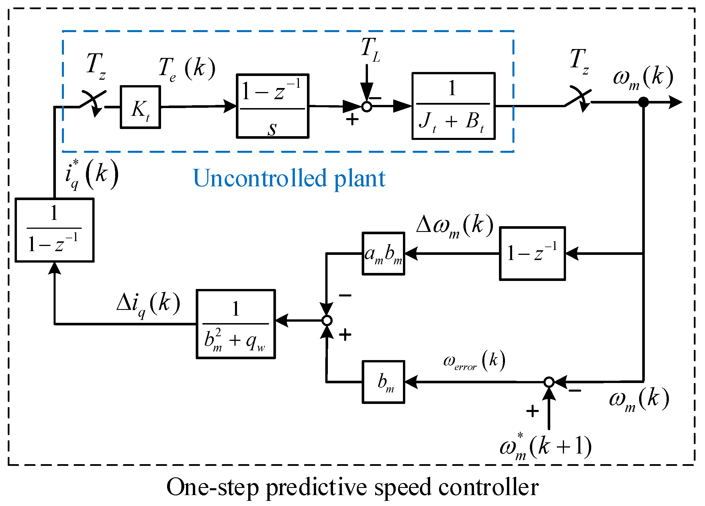
From Equations (40) and (41), one can obtain the block diagram of the one-step predictive speed control which is shown in Figure 6. In this paper, a more complicated two-step predictive speed control has been investigated and compared to the one-step predictive speed control, which is discussed in Equation (31) to (41). The particulars of the two-step predictive speed controller are as follows:

4.2. Two-Step Predictive Speed Controller Design

For a deeper investigation, a two-step predictive speed controller is also investigated in this paper. When we discuss the two-step predictive speed controller, the predictive speed ${\widehat{\omega }}_m(k+1)$ and the predictive speed ${\widehat{\omega }}_m(k+2)$ are both considered.

First, from Equation (38), the predictive speed ${\widehat{\omega }}_m(k+1)$ is developed. Then, one can develop the predictive speed ${\widehat{\omega }}_m(k+2)$ as follows:

$$\begin{gathered} \Delta {\omega }_m(k+2)=a_m\Delta {\omega }_m(k+1)+b_m\Delta i_q(k+1) \\ =a_m[a_m\Delta {\omega }_m(k)+b_m\Delta i_q(k)]+b_m\Delta i_q(k+1) \\ =a_m{}^2\Delta {\omega }_m(k)+a_m{b}_m\Delta i_q(k)+b_m\Delta i_q(k+1) \end{gathered}$$

(42)

Then, the estimated (k + 2)th speed is as follows:

$$\begin{gathered} {\stackrel{{\displaystyle ⌢}}{\omega }}_m(k+2)={\stackrel{{\displaystyle ⌢}}{\omega }}_m(k+1)+\Delta {\omega }_m(k+2) \\ ={\stackrel{{\displaystyle ⌢}}{\omega }}_m(k+1)+a_m{}^2\Delta {\omega }_m(k)+a_m{b}_m\Delta i_q(k)+b_m\Delta i_q(k+1) \\ ={\omega }_m(k)+a_m\Delta {\omega }_m(k)+b_m\Delta i_q(k)+a_m{}^2\Delta {\omega }_m(k)+a_m{b}_m\Delta i_q(k)+b_m\Delta i_q(k+1) \end{gathered}$$

(43)

Combing Equations (42) and (43), we can derive the following equation:

$$\begin{gathered} Y_{sm}=\left[\begin{array}{c}{\stackrel{{\displaystyle ⌢}}{\omega }}_m(k+1)\\ \\ {\stackrel{{\displaystyle ⌢}}{\omega }}_m(k+2)\end{array}\right] \\ =\left[\begin{array}{ccc}{a}_m& & 1\\ & & \\ a_m+a_m{}^2& & 1\end{array}\right]\left[\begin{array}{c}\Delta {\omega }_m(k)\\ \\ {\omega }_m(k)\end{array}\right]+\left[\begin{array}{ccc}{b}_m& & 0\\ & & \\ b_m(1+a_m)& & b_m\end{array}\right]\left[\begin{array}{c}\Delta i_q\left(k\right)\\ \\ \Delta i_q(k+1)\end{array}\right] \\ =F_{sm}{}_{}{X}_{sm}+{\theta }_{sm}\Delta U_{sm} \end{gathered}$$

(44)

with,

$$F_{sm}{}_{}=\left[\begin{array}{ccc}{a}_m& & 1\\ & & \\ a_m+a_m{}^2& & 1\end{array}\right]$$

(45)

and,

$${\theta }_{sm}=\left[\begin{array}{ccc}{b}_m& & 0\\ & & \\ b_m(1+a_m)& & b_m\end{array}\right]$$

(46)

Next, the performance index is defined as follows:

$$J_{sp}={\left[Y_{sm}{}^{*}-Y_{sm}\right]}^T[Y_{sm}{}^{*}-Y_{sm}]+\Delta U_{sm}{}^T\eta \Delta U_{sm}$$

(47)

where $Y_{sm}{}^{*}$, $\eta$, and $\Delta U_{sm}$ are defined as follows:

$$Y_{sm}{}^{*}=\left[\begin{array}{c}{\omega }_m{}^{*}(k+1)\\ \\ {\omega }_m{}^{*}(k+2)\end{array}\right]$$

(48)

In Equation (48), $Y_{sm}{}^{*}$ is the vector that includes the first-step speed command and the second-step speed command. The weighting matrix $\eta$ is:

$$\eta =\left[\begin{array}{ccc}{\eta }_w& & 0\\ & & \\ 0& & {\eta }_w\end{array}\right]$$

(49)

where $\eta$ is the weighting matrix and ${\eta }_w$ is the weighting factor for the first and second q-axis predictive difference-currents. The control input currents at sampling intervals k and k + 1 are:

$$\Delta U_{sm}=\left[\begin{array}{c}\Delta i_q(k)\\ \\ \Delta i_q(k+1)\end{array}\right]$$

(50)

where $\Delta U_{sm}$ are the control input currents at sampling intervals k and k + 1. After that, by taking the partial difference, one can obtain the following equation:

$$\frac{\partial J_{sp}}{\partial \Delta U_{sm}}=(-2{\theta }_{sm}{}^T(Y_m{}^{*}-F_{sm}{X}_{sm}(k))+2{({\theta }_{sm}{}^T{\theta }_{sm}+\eta )}_{}\Delta U_{sm}(k))=0$$

(51)

From (51), the optimal predictive control input can be expressed as follows:

$$\Delta U_{sm}={({\theta }_{sm}{}^T{\theta }_{sm}+\eta )}^{-1}({\theta }_{sm}{}^T{Y}_{sm}{}^{*}(k)-{\theta }_{sm}{}^T{F}_{sm}{X}_{sm}(k))$$

(52)

The relative results are as follows:

$${\theta }_{sm}{}^T{\theta }_{sm}+\eta =\left[\begin{array}{ccc}{a}_m^2{b}_m^2+2a_m{b}_m^2+2b_m^2+{\eta }_w& & a_m{b}_m{}^2+b_m{}^2\\ & & \\ a_m{b}_m{}^2+b_m{}^2& & b_m{}^2+{\eta }_w\end{array}\right]$$

(53)

$$\begin{gathered} {\theta }_{sm}{}^T{Y}_m{}^{*}=\left[\begin{array}{ccc}{b}_m& & b_m(1+a_m)\\ & & \\ 0& & b_m\end{array}\right]\left[\begin{array}{c}{\omega }_m{}^{*}(k+1)\\ \\ {\omega }_m{}^{*}(k+2)\end{array}\right] \\ =\left[\begin{array}{c}{b}_m{\omega }_m{}^{*}(k+1)+b_m(1+a_m){\omega }_m{}^{*}(k+2)\\ \\ b_m{\omega }_m{}^{*}(k+2)\end{array}\right] \end{gathered}$$

(54)

and,

$$\begin{gathered} {\theta }_{sm}{}^T{F}_{sm}{X}_{sm}(k)=\left[\begin{array}{ccc}{b}_m& & b_m(1+a_m)\\ & & \\ 0& & b_m\end{array}\right]\left[\begin{array}{ccc}{a}_m& & 1\\ & & \\ a_m+a_m{}^2& & 1\end{array}\right]\left[\begin{array}{c}\Delta {\omega }_m(k)\\ \\ {\omega }_m(k)\end{array}\right] \\ =\left[\begin{array}{c}[2\left(a_m{b}_m+a_m^2{b}_m\right)\Delta {\omega }_m(k)+\left[b_m+b_m{(1+a_m)}_{}\right]{\omega }_m(k)\\ \\ b_m(a_m+a_m{}^2)\Delta {\omega }_m(k)+b_m{\omega }_m(k)\end{array}\right] \end{gathered}$$

(55)

Substituting (53), (54), and (55) into (52), one can derive the following equations:

$$\begin{gathered} \Delta U_{sm}(\mathrm{k})=\left[\begin{array}{c}\Delta i_q(k)\\ \\ \Delta i_q(k+1)\end{array}\right]=\frac{\left[\begin{array}{ccc}2b_m{}^2+{\eta }_w& & -a_m{b}_m{}^2-b_m^2\\ & & \\ -a_m{b}_m{}^2-b_m^2& & a_m^2{b}_m^2+2a_m^2{b}_m^2+2b_s^2+{\eta }_w\end{array}\right]}{b_m{}^4+{\eta }_w{}^2+b_m^2{\eta }_w\left(a_m^2+2a_m+3\right)} \\ \left[\begin{array}{c}{b}_m{\omega }_m{}^{*}(k+1)+b_m(1+a_m){\omega }_m{}^{*}(k+2)-2\left(a_m{b}_m+a_m^2{b}_m\right)\Delta {\omega }_m(k)-\left[b_m+b_m(1+a_m)\right]{\omega }_m(k)\\ \\ b_m{\omega }_m{}^{*}(k+2)-[b_m(a_m+a_m{}^2)]\Delta {\omega }_m(k)-b_m{\omega }_m(k)\end{array}\right] \\ =\frac{1}{Z}\left[\begin{array}{c}\Psi +\Theta \\ \\ \Phi +{\rm N}\end{array}\right] \end{gathered}$$

(56)

and,

$$Z=b_m{}^4+{\eta }_w{}^2+b_m^2{\eta }_w\left(a_m^2+2a_m+3\right)$$

(57)

$$\begin{array}{ll}\Psi & =\left(2b_m^2+{\eta }_w\right)\{b_m{\omega }_m{}^{*}(k+1)+b_m(1+a_m){\omega }_m{}^{*}(k+2)\\ & -2\left(b_m{a}_m+b_m{a}_m{}^2\right)\Delta {\omega }_m(k)-\left[b_m+b_m(1+a_m)\right]{\omega }_m(k)\}\end{array}$$

(58)

$$\Theta =\left[-a_m{b}_m{}^2-b_m^2\right]\{b_m{\omega }_m{}^{*}(k+2)-b_m(a_m+a_m{}^2)\Delta {\omega }_m(k)-b_m{\omega }_m(k)\}$$

(59)

$$\begin{array}{ll}\Phi & =\left[-a_m{b}_m{}^2-b_m^2\right]\{b_m{\omega }_m{}^{*}(k+1)+b_m(1+a_m){\omega }_m{}^{*}(k+2)\\ & -2\left(b_m{a}_m+b_m{a}_m{}^2\right)\Delta {\omega }_m(k)-\left[b_m+b_m(1+a_m)\right]{\omega }_m(k)\}\end{array}$$

(60)

and,

$${\rm N}=\left[a_m{}^2{b}_m{}^2+2b_m^2+2a_m{b}_m{}^2+{\eta }_w\right]\{b_m{\omega }_m{}^{*}(k+2)-b_m(a_m+a_m{}^2)\Delta {\omega }_m(k)-b_m{\omega }_m(k)\}$$

(61)

Next, the q-axis current command at the k-th sampling interval is as follows:

$$i_q^{*}(k)=i_q^{*}(k-1)+\Delta i_q(k)$$

(62)

By using the same method, the (k + 1)th q-axis current command is shown in the following equation:

$$i_q^{*}(k+1)=i_q^{*}(k)+\Delta i_q(k+1)$$

(63)

The output q-axis current command sends out only one value for each sampling interval. As a result, we can combine Equations (62) and (63). Then, the final q-axis current using the two-step predictive speed controller is defined as follows:

$$i_q{}^{*}{(k)}_{-2step}=\rho i_q{}^{*}(k)+{(1-\rho )}_{}{i}_q{}^{*}(k+1)$$

(64)

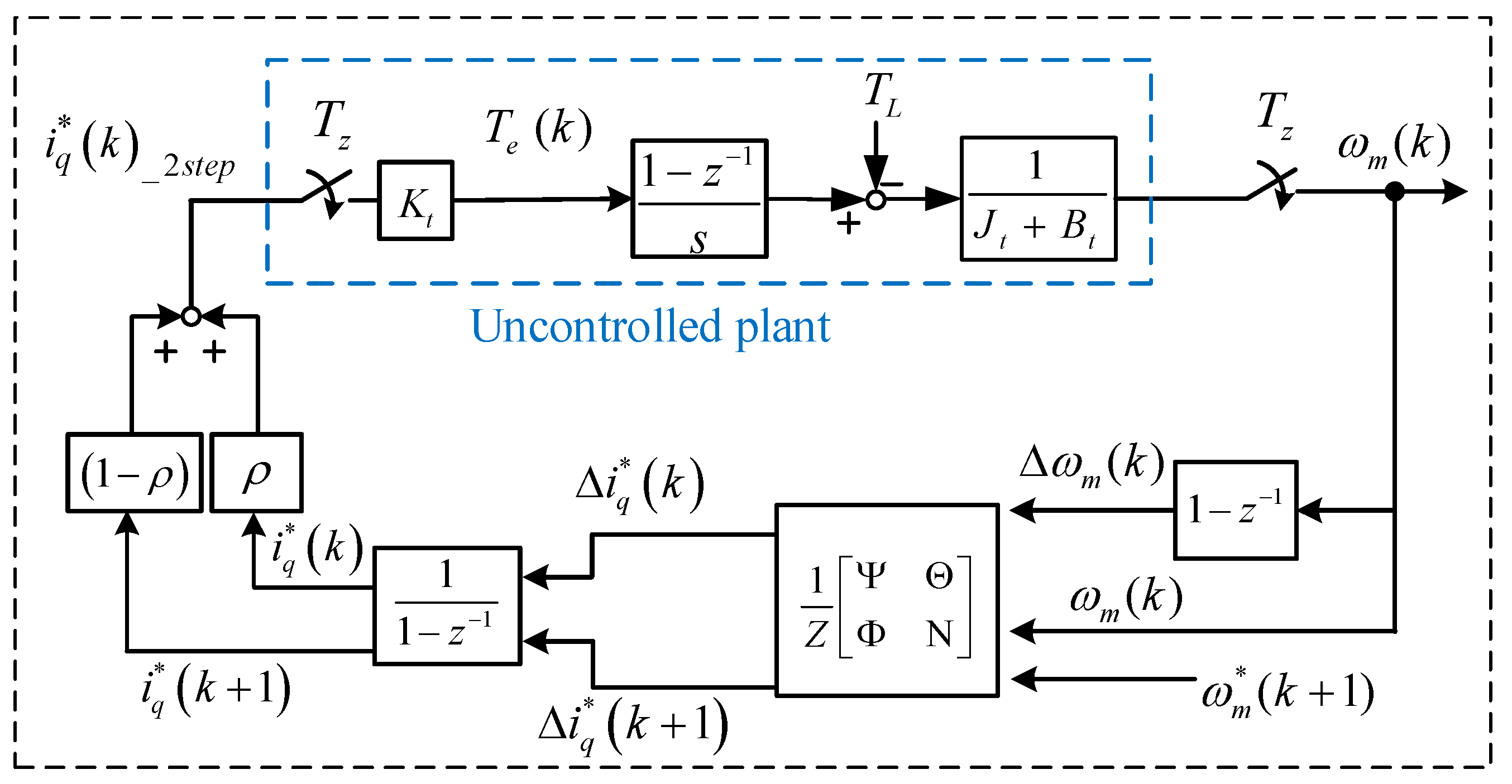
From Equation (56) to (64), we can obtain the block diagram of the two-step predictive speed control. Figure 7 shows the block diagram of two-step predictive speed control system.

5. Predictive Current Controller Design

The predictive current controller is developed by using a similar method as the predictive speed controller. First, the differential equations of the d-axis and q-axis currents are as follows:

$$\frac{d}{dt}{i}_d=\frac{1}{L_d}\left(v_d-r_s{i}_d+{\omega }_e{L}_q{i}_q\right)$$

(65)

and,

$$\frac{d}{dt}{i}_q=\frac{1}{L_q}\left(v_q-r_s{i}_q+{\omega }_e(L_d{i}_d+{\lambda }_m)\right)$$

(66)

By inserting these two zero-order hold devices into the d-q axis currents and then taking the z-transformation, we obtain the following equation:

$$\left[\begin{array}{c}{i}_d\left(k+1\right)\\ i_q\left(k+1\right)\end{array}\right]=\left[\begin{array}{cc}{a}_d& 0\\ 0& a_q\end{array}\right]\left[\begin{array}{c}{i}_d\left(k\right)\\ i_q\left(k\right)\end{array}\right]+\left[\begin{array}{cc}{b}_d& 0\\ 0& b_q\end{array}\right]\left[\begin{array}{c}{v}_d\left(k\right)+{\omega }_e\left(k\right)L_q{i}_q\left(k\right)\\ v_q\left(k\right)-{\omega }_e\left(k\right)\left(L_d{i}_d\left(k\right)+{\lambda }_m\right)\end{array}\right]$$

(67)

The parameters $a_d$, $a_q$, $b_d$, and $b_q$ are as follows:

$$a_d=e^{-\frac{r_s{T}_c}{L_d}}$$

(68)

$$b_d=\frac{1}{r_s}(1-e^{-\frac{r_s}{L_d}{T}_c})$$

(69)

$$a_q=e^{-\frac{r_s{T}_c}{L_q}}$$

(70)

and,

$$b_q=\frac{1}{r_s}(1-e^{-\frac{r_s}{L_q}{T}_c})$$

(71)

Next, we can define the control input $u_d(k)$ and $u_q(k)$ as the following two equations:

$$u_d(k)=v_d(k)+{\omega }_e{(k)}_{}{L}_q{}_{}{i}_q(k)$$

(72)

and,

$$u_q(k)=v_q(k)-{\omega }_e{(k)}_{}(L_d{i}_d(k)+{\lambda }_m(k))$$

(73)

Substituting Equations (72) and (73) into (67), we can obtain a new and simplified state-variable presentation equation as follows:

$$\left[\begin{array}{c}{x}_d\left(k+1\right)\\ x_q\left(k+1\right)\end{array}\right]=\left[\begin{array}{cc}{a}_d& 0\\ 0& a_q\end{array}\right]\left[\begin{array}{c}{x}_d\left(k\right)\\ x_q\left(k\right)\end{array}\right]+\left[\begin{array}{cc}{b}_d& 0\\ 0& b_q\end{array}\right]\left[\begin{array}{c}{u}_d(k)\\ u_q(k)\end{array}\right]$$

(74)

where $x_d\left(k\right)$ is the new state variable of $i_d\left(k\right)$, and $x_q\left(k\right)$ is the new state variable of $i_q\left(k\right)$. Equation (74) can then be rewritten as the new state-variable vector presentation as the following equations:

$$X_{cm}\left(k+1\right)=A_{cm}{X}_{cm}\left(k\right)+B_{cm}{U}_{cm}\left(k\right)$$

(75)

and,

$$X_{cm}\left(k\right)=\left[\begin{array}{c}{x}_d\left(k\right)\\ x_q\left(k\right)\end{array}\right]$$

(76)

$$A_{cm}=\left[\begin{array}{cc}{a}_d& 0\\ 0& a_q\end{array}\right]$$

(77)

$$B_{cm}=\left[\begin{array}{cc}{b}_d& 0\\ 0& b_q\end{array}\right]$$

(78)

and,

$$U_{cm}\left(k\right)=\left[\begin{array}{c}{u}_d(k)\\ u_q(k)\end{array}\right]$$

(79)

The new output equation of the state-variable vector presentation is as follows:

$$Y_{cm}=\left[\begin{array}{c}{y}_d\left(k\right)\\ y_q\left(k\right)\end{array}\right]=\left[\begin{array}{cc}1& 0\\ 0& 1\end{array}\right]\left[\begin{array}{c}{x}_d\left(k\right)\\ x_q\left(k\right)\end{array}\right]$$

(80)

Then, we can define the difference of the state variable as follows:

$$\begin{array}{ll}\Delta X_{cm}(k+1)& =X_{cm}(k+1)-X_{cm}(k)\\ & =A_{cm}\Delta X_{cm}(k)+B_{cm}\Delta U_{cm}(k)\end{array}$$

(81)

where $\Delta X_{cm}\left(k\right)$ is the difference of the state variables, and $\Delta U_{cm}\left(k\right)$ is the difference of the output variables. After that, we can define the augmented state variables as follows:

$$\begin{array}{l}{X}_m(k+1)=\left[\begin{array}{c}\Delta X_{cm}(k+1)\\ Y_{cm}(k+1)\end{array}\right]=A_m{X}_m(k)+B_m\Delta U_{cm}(k)\\ \end{array}$$

(82)

with:

$$A_m=\left[\begin{array}{cc}{A}_{cm}& 0_{cm}^T\\ A_{cm}& 1\end{array}\right]$$

(83)

$$X_m(k)=\left[\begin{array}{c}\Delta X_{cm}(k)\\ Y_{cm}(k)\end{array}\right]$$

(84)

and,

$$B_m=\left[\begin{array}{c}{B}_{cm}\\ B_{cm}\end{array}\right]$$

(85)

Next, we can define the output $Y_m(k+1)$ of the augmented model as follows:

$$\begin{array}{ll}{Y}_m(k+1)& =\left[\begin{array}{cc}{0}_{cm}^T& 1\end{array}\right]X_m(k+1)\\ & =C_m{X}_m(k+1)\end{array}$$

(86)

The performance index of the current-loop controllers is defined as follows [26]:

$$J_c={\left(X_{cm}^{*}\left(k+1\right)-Y_m\left(k+1\right)\right)}^2+q\Delta U_{cm}^2\left(k\right)$$

(87)

where $q$ is the weighting factor. By taking the differential of the performance index to $\Delta U_{cm}\left(k\right)$, and then by assuming the result to be zero, one can derive the following optimal difference control input $\Delta U_{cm}^{*}\left(k\right)$ as follows:

$$\begin{array}{l}\Delta U_{cm}^{*}\left(k\right)={\left(B_{cm}^2+q\right)}^{-1}[B_{cm}{X}_{cm}^{*}\left(k+1\right)\\ -A_{cm}{B}_{cm}\Delta X_{cm}\left(k\right)-B_{cm}{Y}_{cm}\left(k\right)]\end{array}$$

(88)

From Equation (88), the $\Delta v_d^{*}\left(k\right)$ and $\Delta v_q^{*}\left(k\right)$ can be expressed as the following equations:

$$\begin{array}{ll}\Delta v_d^{*}\left(k\right)& =\frac{b_d\left(i_d^{*}\left(k+1\right)-i_d\left(k\right)\right)-a_d{b}_d\Delta i_d\left(k\right)}{b_d^2+q}\\ & -\Delta {\omega }_e\left(k\right)L_q\Delta i_q\left(k\right)\end{array}$$

(89)

and,

$$\begin{array}{ll}\Delta v_q^{*}\left(k\right)& =\frac{b_q\left(i_q^{*}\left(k+1\right)-i_q\left(k\right)\right)-a_q{b}_q\Delta i_q\left(k\right)}{b_q^2+q}\\ & -\Delta {\omega }_e\left(k\right)\left(L_d\Delta i_d\left(k\right)+{\lambda }_m\right)\end{array}$$

(90)

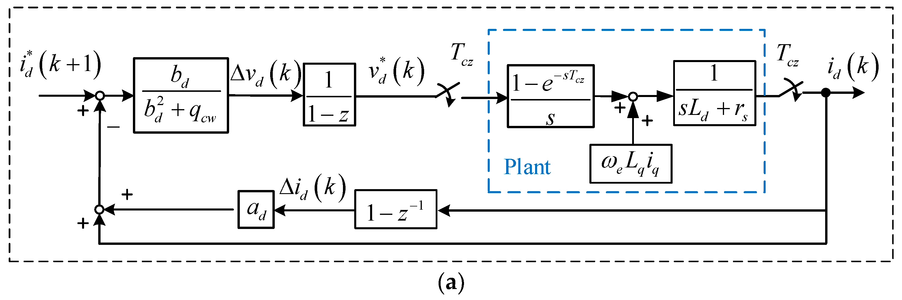
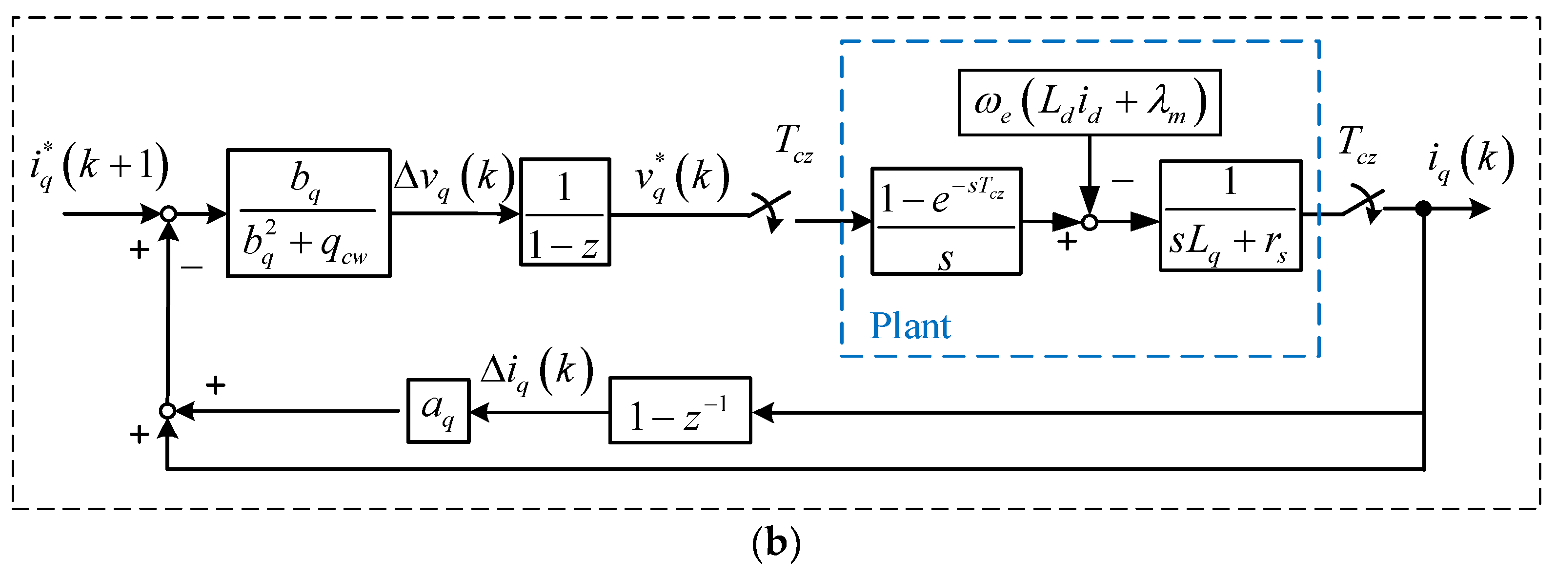
Finally, from Equations (89) and (90), we can develop the block diagrams of the d-axis current controller and the q-axis current controller as in Figure 8a,b.

6. Implementation

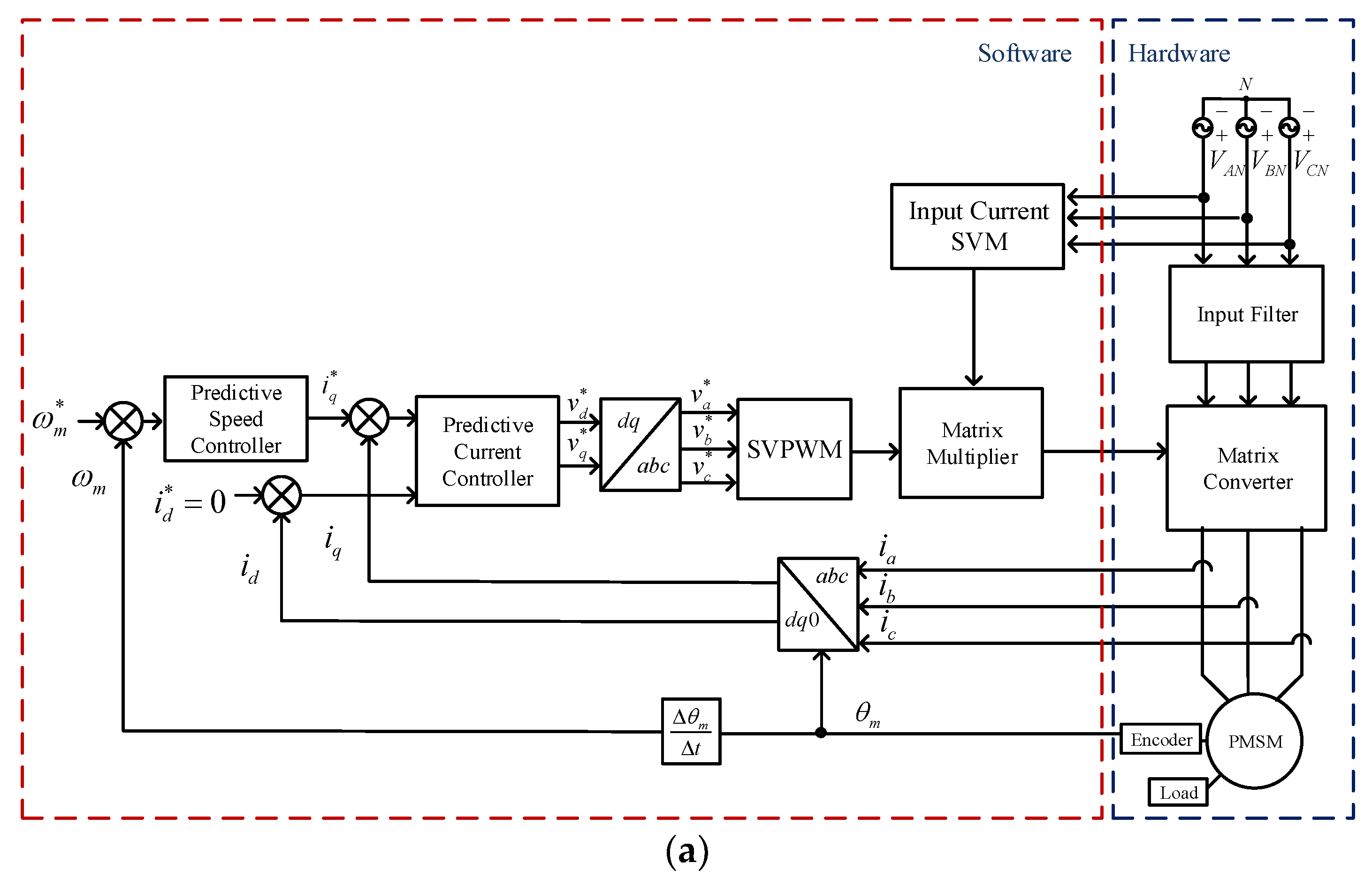
A digital signal processor (DSP), type SH 7237 (manufactured by Renesas Electronics Corporation, Tokyo, Japan), and an FPGA, type 10M16SAU16917G (manufactured by Intel Corporation, Santa Clara, CA, USA), were used to execute the control algorithms. The sampling interval of the speed-loop was 1 ms, and the sampling interval of the current-loop was 100 μs. The switching frequency of the matrix converter was 10 kHz. The PMSM was an 8-pole motor, which had a 2000 r/min rated speed, 9.55 N·m of rated torque, 9 A of rated current, 0.58 Ω of stator resistance, 1.3 mH of d-axis inductance, 1.7 mH of q-axis inductance, 0.003 N·m·s/rad of inertia, and a 1.14 N·m/A torque constant. The three-phase input filter of method 1 had the following parameters: $R_d$ = 15 Ω, $L_f$ = 1.5 mH, and $C_f$ = 6.8 μF. In addition, the three-phase input filter of method 2 had the following parameters: $R_d$ = 22 Ω, $L_f$ = 1.5 mH, and $C_f$ = 4.7 μF. Figure 9a shows the software and hardware block diagrams of the control system. Figure 9b shows the circuits for a matrix converter, including a clamped circuit, some drivers, a matrix converter, an AC/DC power supply, and a control circuit.

7. Experimental Results

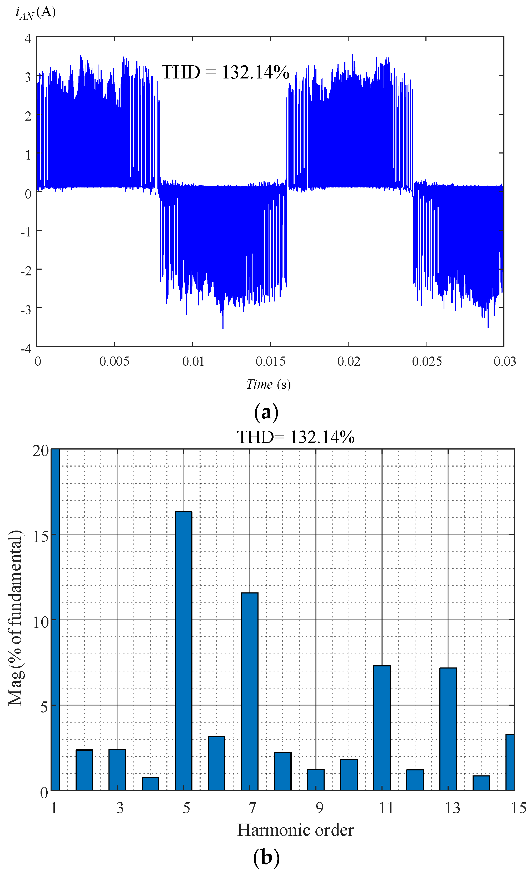
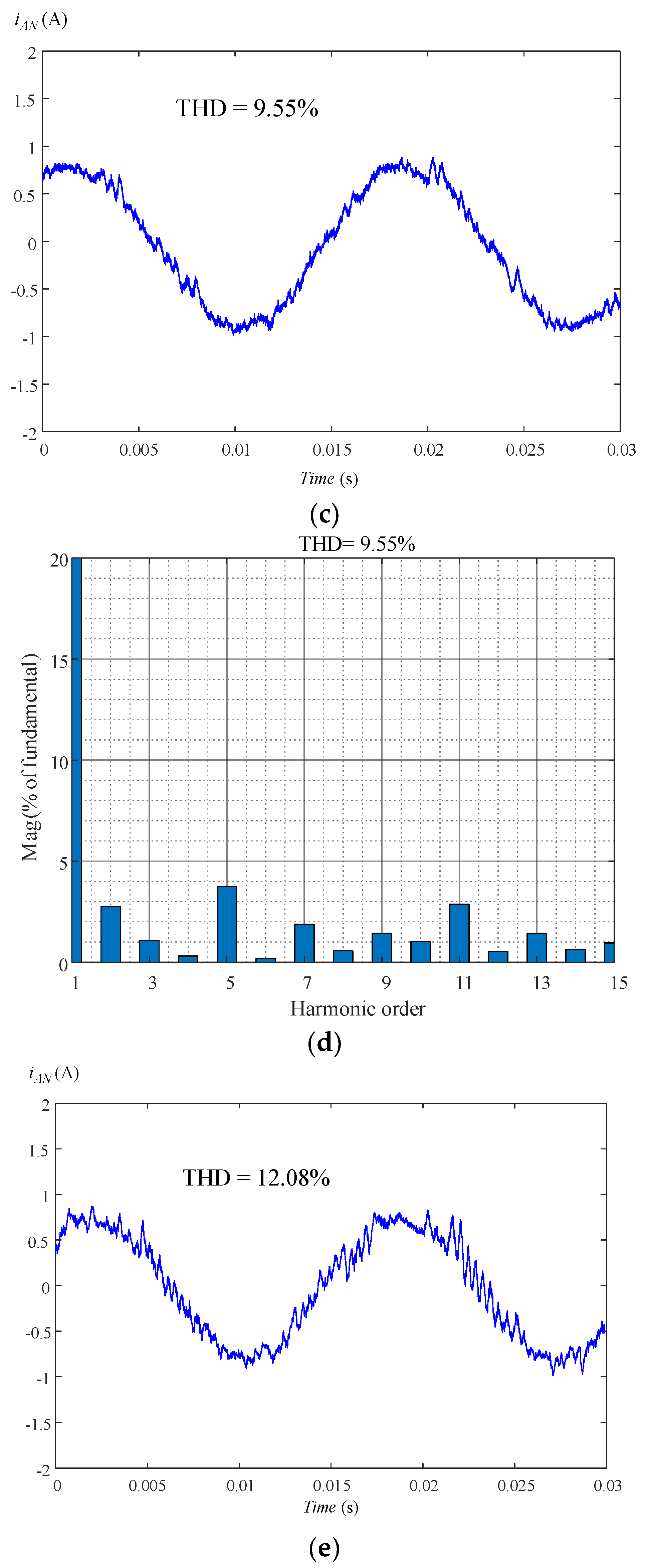
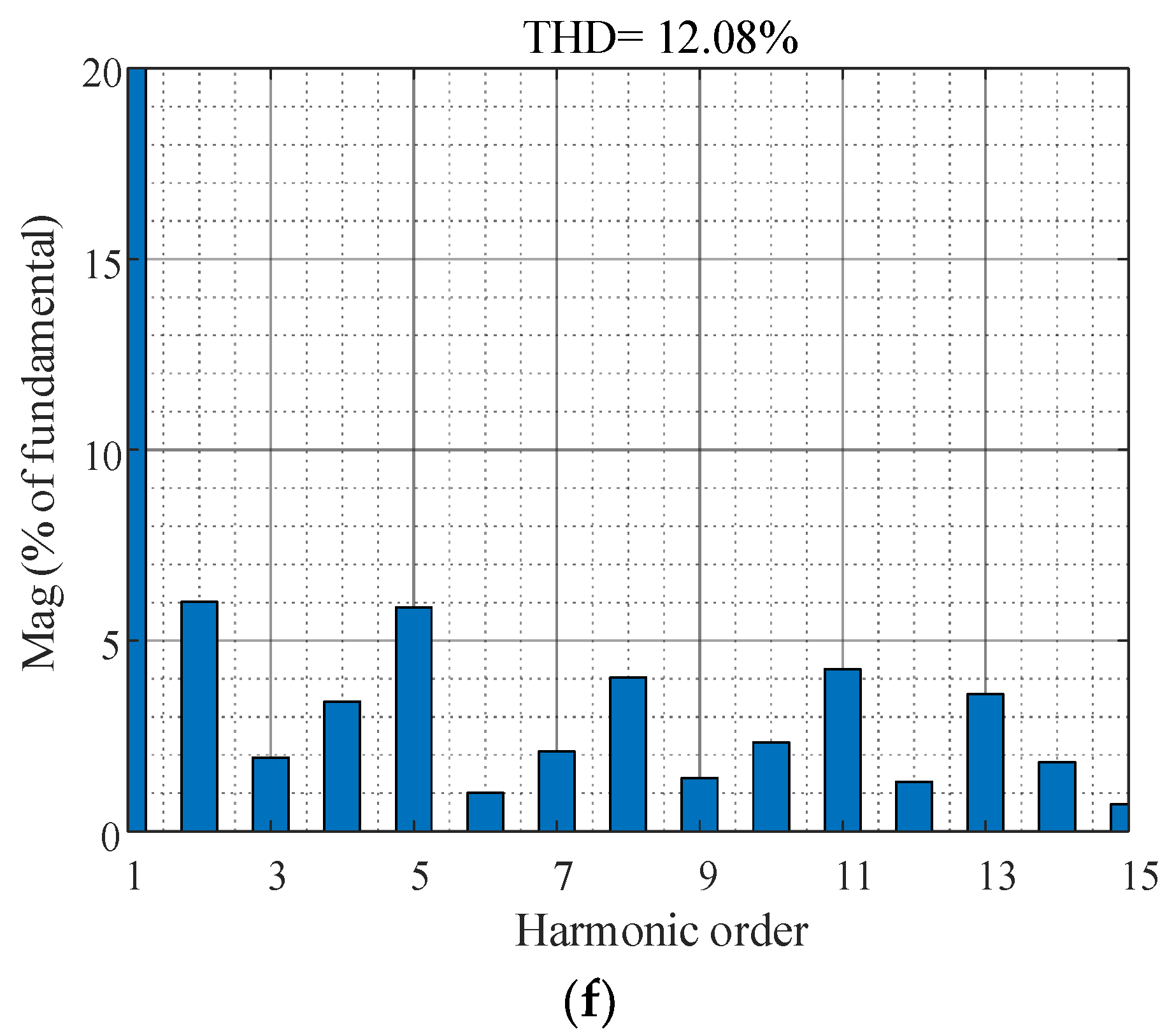
Several experimental results are shown here. Figure 10a demonstrates the measured input A-phase current of the matrix converter without using an input filter. The input A-phase current is close to a square-wave high-frequency PWM current, which has a 132.14% THD. Two simplified three-phase input AC filter design methods were proposed without using computer simulations. Figure 10c demonstrates the measured A-phase current using the proposed method 1 of the three-phase input AC filter, in which the parameters include ${\lambda }_1$ = 0.11, ${\lambda }_2$ = 0.019, and ${\lambda }_3$ = 0.0006. The measured A-phase current is nearly a sinusoidal waveform with a 9.55% THD. Figure 10e demonstrates the measured A-phase current using the proposed method 2 input three-phase AC filter, in which the parameters include ${\omega }_{res}$ = 12,570 rad/s, $Q_{res}$ = 1.23, and $\xi$ = 0.4. The A-phase current using method 2 includes a 12.08% THD. As we can observe, the current without using an input filter has the highest THD. The major reason is that the high-frequency PWM current creates a lot of harmonic currents. The proposed method 1 of the three-phase input AC filter design provides lower THD than the proposed method 2. The major reason is that method 1 focuses on harmonic currents and voltages; method 2, however, focuses on frequency responses.

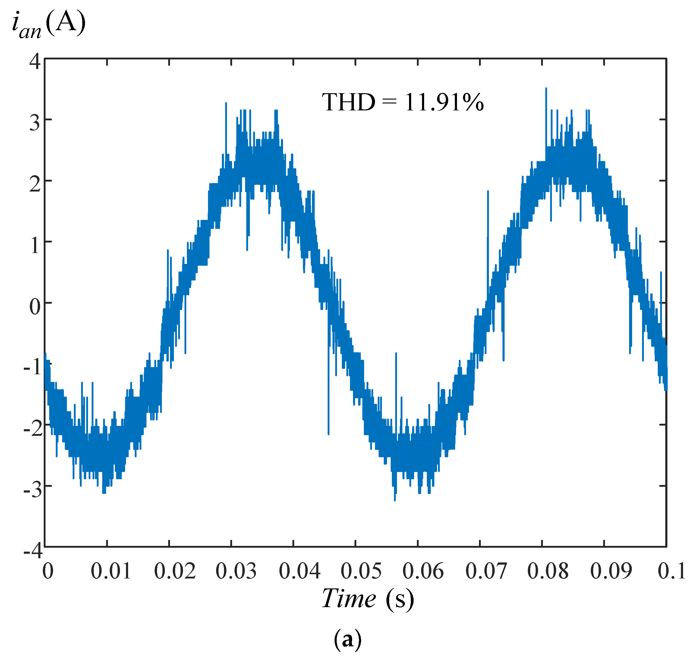
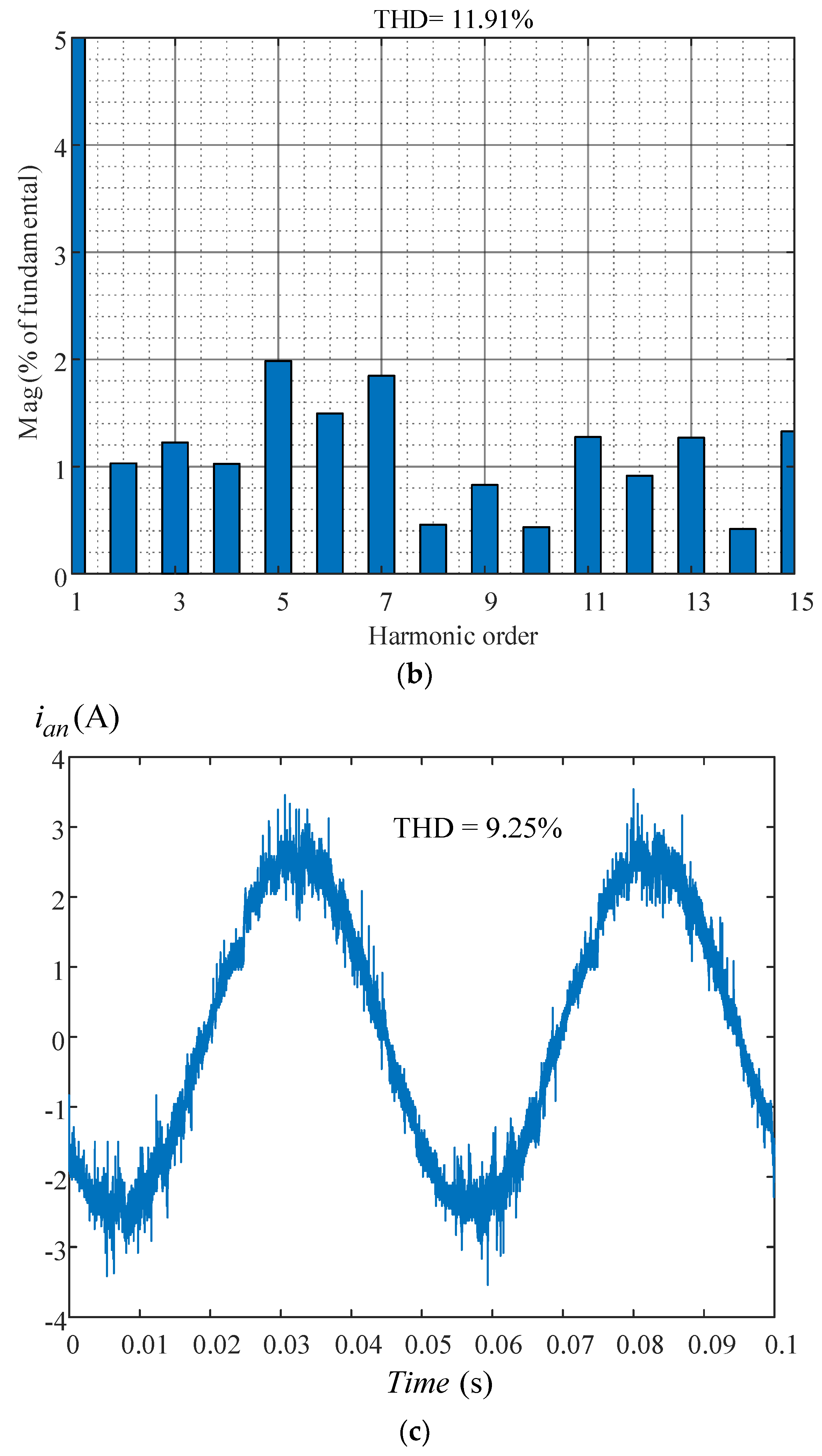
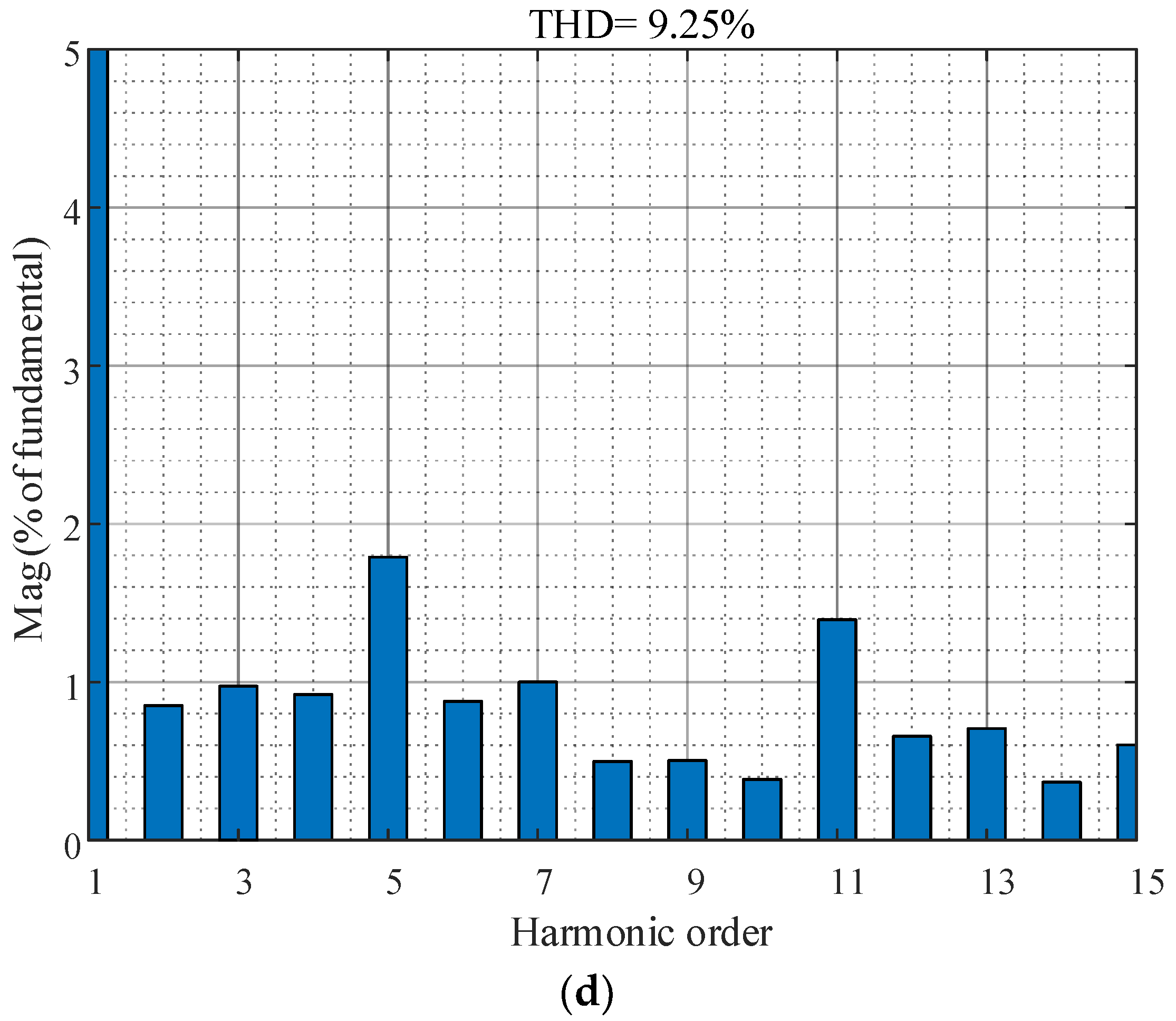
Figure 11a demonstrates the measured output currents of the a-phase matrix converter using a PI current controller, which produces an 11.91% THD. Figure 11c demonstrates the measured output currents of the a-phase matrix converter using a predictive current controller, which has a 9.25% THD, which is lower than the THD of the PI current controller.

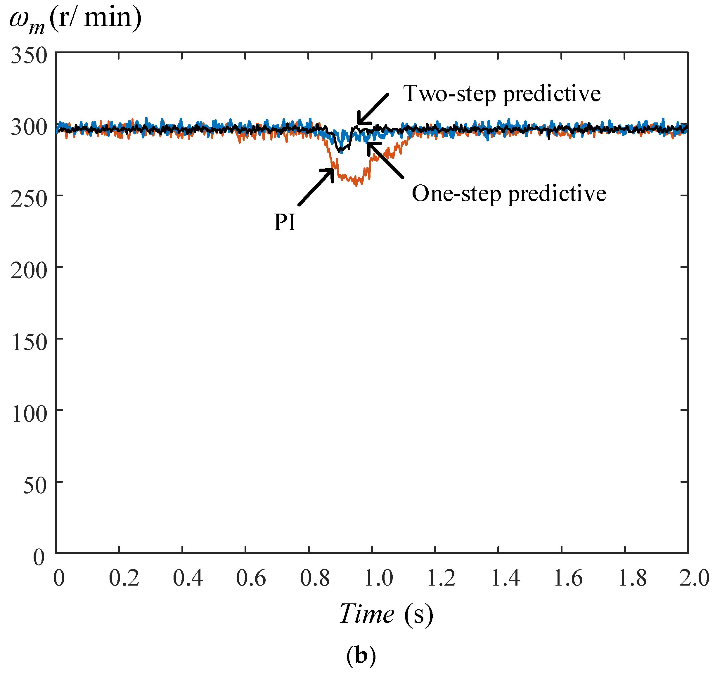
Figure 12a illustrates the measured 300 r/min step-input speed responses by using a PI controller, a one-step predictive speed controller, and a two-step predictive speed controller. The PI controller is designed by pole assignment with two major poles $P_1$ = −10.6 + j7.5 and $P_2$ = −10.6 − j7.5. As we can observe, the PI controller provides the highest overshoot among the three different speed controllers. The one-step predictive speed controller, which chooses a weighting factor q = 0.25, has the quickest transient response when compared to the two-step predictive speed controller and the PI controller. The two-step predictive speed controller, which chooses a weighting factor $\eta =\left[\begin{array}{cc}0.25& 0\\ 0& 0.25\end{array}\right]$ and $\rho$ = 0.5, has the lowest overshoot but the slowest transient response when compared to the PI controller and the one-step predictive speed controller. Figure 12b illustrates the load disturbance responses at 300 r/min with a 2 N·m external load. The one-step predictive controller provides the smallest speed drop and the fastest recovery time relative to the PI controller and the two-step predictive controller. However, the two-step predictive controller provides fewer steady-state errors than the PI controller and the one-step predictive speed controller.

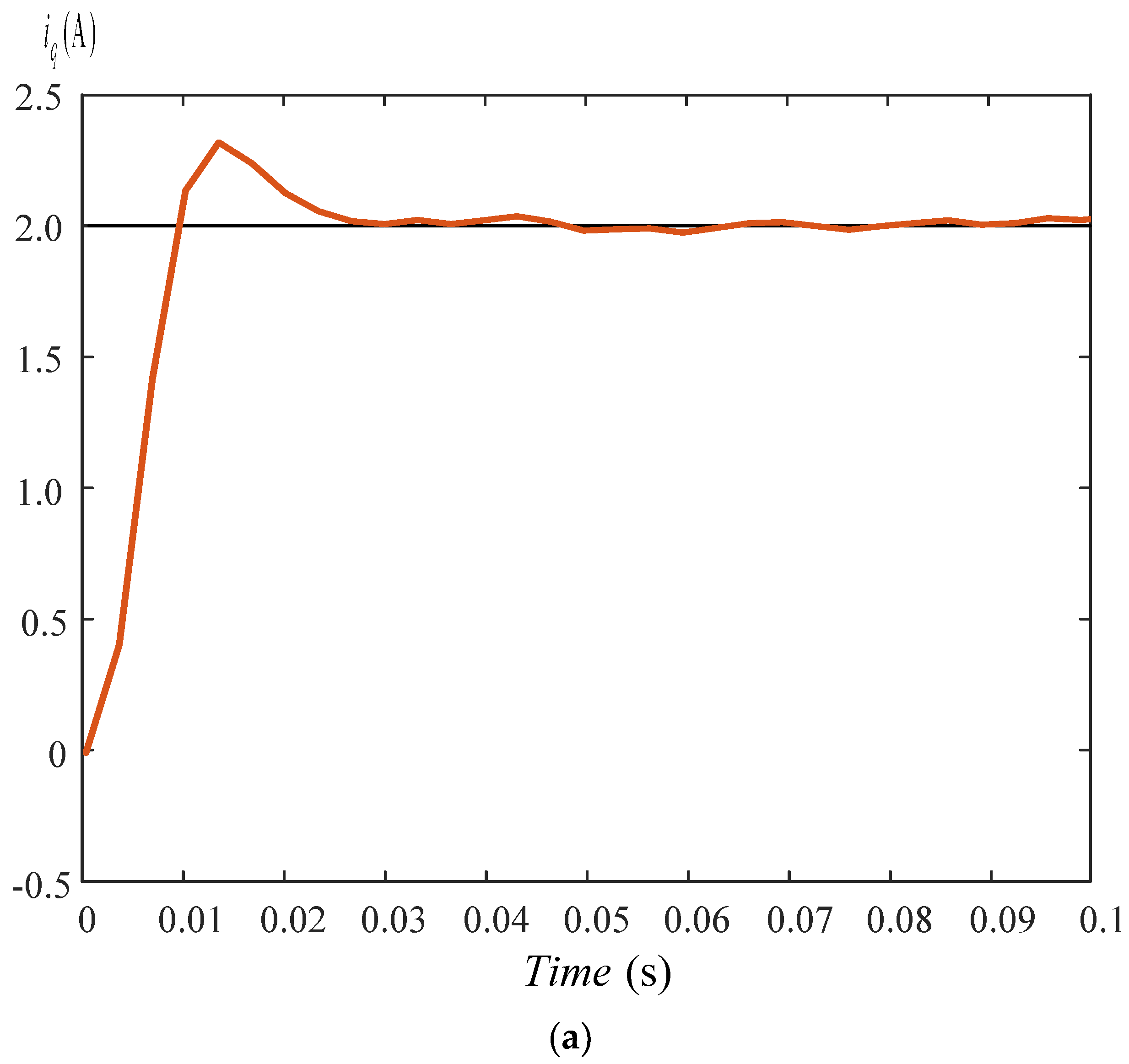
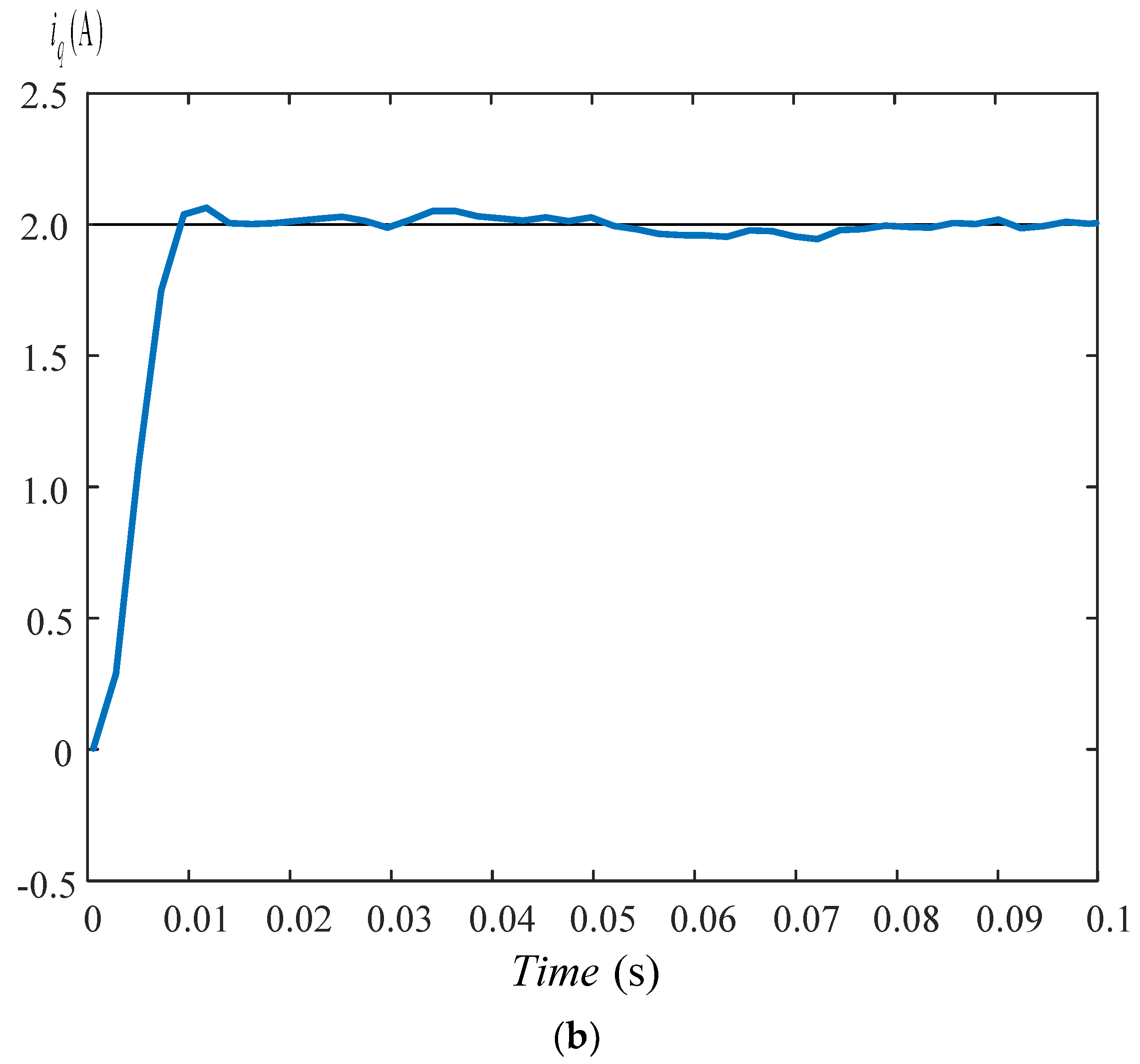
Figure 13a demonstrates the measured q-axis current response by using the PI controller, which has a higher overshoot and slower response than the one-step predictive current controller. Figure 13b demonstrates the measured q-axis current response by using the one-step predictive controller. As can be observed, the one-step predictive current controller performs better than the PI controller again, including faster transient responses and lower overshoot.

Table 2. Comparison of input harmonic currents.

		5th Harmonic	7th Harmonic	THD
Without input filters		16.26%	11.61%	132.14%
Method 1		3.73%	1.87%	9.55%
Method 2		5.87%	2.09%	12.08%

shows the comparison of the input harmonic currents. Method 1 has fewer input harmonic currents than method 2.

Table 3. Comparison of speed responses.

	Command	PI	One-Step Predictive	Two-Step Predictive
Controller
Step speed command 300 r/min	Rise time	0.15 s	0.13 s	0.17 s
	Settling time	0.4 s	0.24 s	0.26 s
	Overshoot	6.33%	2%	1%
	Steady state error	$\pm$2 r/min	$\pm$2 r/min	$\pm$1 r/min
Load-disturbance 2 N-m	Recovery time	0.28 s	0.17 s	0.2 s
	Speed drop	48 r/min	24 r/min	23 r/min

shows the comparison of the speed responses. The one-step predictive speed controller provides quicker transient responses and quicker recovery time. However, the two-step predictive speed controller provides fewer speed drops and smaller overshoots than any other controller.

8. Conclusions

In this paper, two different design methods, which are simpler than the traditional numeric methods, using a computer for a three-phase input AC filter for matrix-converter PMSM-drive systems, are investigated and compared. The first method requires only analytic processes, which is simpler than the traditional numeric method using a computer. The second method uses frequency responses to determine the R-L-C parameters of the AC filter. In addition, a two-step predictive speed controller and a one-step predictive speed controller are investigated to improve the dynamic responses of speed-loop control systems. Moreover, a predictive current controller is designed to provide smaller harmonic currents than a PI current controller. Experimental results show that the proposed methods can effectively improve the performance of matrix converter-based PMSM drive systems, including obvious improvements in the input AC harmonic currents, output AC harmonic currents, and dynamic responses.

References

- Rodriguez, J.; Rivera, M.; Kolar, J.W.; Wheeler, P. A Review of Control and Modulation Methods for Matrix Converters. IEEE Trans. Ind. Electron. 2011, 59, 58–70. [Google Scholar] [CrossRef]
- Lei, J.; Zhou, B.; Qin, X.; Wei, J.; Bian, J. Active damping control strategy of matrix converter via modifying input reference currents. IEEE Trans. Power Electron. 2014, 30, 5260–5271. [Google Scholar] [CrossRef]
- Sahoo, A.K.; Basu, K.; Mohan, N. Systematic Input Filter Design of Matrix Converter by Analytical Estimation of RMS Current Ripple. IEEE Trans. Ind. Electron. 2014, 62, 132–143. [Google Scholar] [CrossRef]
- Oser, D.; Mohan, N. A matrix converter ride-through configuration using input filter capacitors as an energy exchange mechanism. IEEE Trans. Power Electron. 2015, 30, 4377–4385. [Google Scholar] [CrossRef]
- Dasgupta, A.; Sensarma, P. Filter Design of Direct Matrix Converter for Synchronous Applications. IEEE Trans. Ind. Electron. 2014, 61, 6483–6493. [Google Scholar] [CrossRef]
- Kume, T.; Yamada, K.; Higuchi, T.; Yamamoto, E.; Hara, H.; Sawa, T.; Swamy, M.M. Integrated filters and their combined effects in matrix converter. IEEE Trans. Ind. Appl. 2007, 43, 571–581. [Google Scholar] [CrossRef]
- Liu, S.; Ge, B.; Liu, Y.; Haitham, A.R.; Balog, R.S.; Sun, H. Modeling, analysis, and parameters design of LC-filter-integrated quasi-Z-source indirect matrix converter. IEEE Trans. Power Electron. 2016, 31, 7544–7555. [Google Scholar] [CrossRef]
- Deng, W.; Li, S. Direct Torque Control of Matrix Converter-Fed PMSM Drives Using Multidimensional Switching Table for Common-Mode Voltage Minimization. IEEE Trans. Power Electron. 2020, 36, 683–690. [Google Scholar] [CrossRef]
- Zhang, J.; Li, L.; Dorrell, D.G.; Guo, Y. Modified PI controller with improved steady-state performance and comparison with PR controller on direct matrix converters. Chin. J. Electr. Eng. 2019, 5, 53–66. [Google Scholar] [CrossRef]
- Mubarok, M.S.; Liu, T.-H. Implementation of Predictive Controllers for Matrix-Converter-Based Interior Permanent Magnet Synchronous Motor Position Control Systems. IEEE J. Emerg. Sel. Top. Power Electron. 2018, 7, 261–273. [Google Scholar] [CrossRef]
- Siami, M.; Khaburi, D.A.; Rodriguez, J. Simplified Finite Control Set-Model Predictive Control for Matrix Converter-Fed PMSM Drives. IEEE Trans. Power Electron. 2017, 33, 2438–2446. [Google Scholar] [CrossRef]
- Xia, C.; Zhao, J.; Yan, Y.; Shi, T. A Novel Direct Torque Control of Matrix Converter-Fed PMSM Drives Using Duty Cycle Control for Torque Ripple Reduction. IEEE Trans. Ind. Electron. 2013, 61, 2700–2713. [Google Scholar] [CrossRef]
- Nguyen-Duy, K.; Liu, T.-H.; Chen, D.-F.; Hung, J.Y. Improvement of Matrix Converter Drive Reliability by Online Fault Detection and a Fault-Tolerant Switching Strategy. IEEE Trans. Ind. Electron. 2011, 59, 244–256. [Google Scholar] [CrossRef]
- Friedli, T.; Kolar, J.W.; Rodriguez, J.; Wheeler, P. Comparative Evaluation of Three-Phase AC–AC Matrix Converter and Voltage DC-Link Back-to-Back Converter Systems. IEEE Trans. Ind. Electron. 2011, 59, 4487–4510. [Google Scholar] [CrossRef]
- Di, Z.; Xu, D.; Tarisciotti, L.; Wheeler, P. A Novel Predictive Control Method with Optimal Switching Sequence and Filter Resonance Suppression for Two-Stage Matrix Converter. Energies 2021, 14, 3652. [Google Scholar] [CrossRef]
- Li, S.; Wang, Z.; Yan, Y.; Shi, T. Finite Set Model Predictive Control of a Dual-Motor Torque Synchronization System Fed by an Indirect Matrix Converter. Energies 2021, 14, 1325. [Google Scholar] [CrossRef]
- Di, Z.; Xu, D.; Zhang, K. Continuous Control Set Model Predictive Control for an Indirect Matrix Converter. Energies 2021, 14, 4114. [Google Scholar] [CrossRef]
- Dendouga, A. Conventional and Second Order Sliding Mode Control of Permanent Magnet Synchronous Motor Fed by Direct Matrix Converter: Comparative Study. Energies 2020, 13, 5093. [Google Scholar] [CrossRef]
- Bu, H.; Cho, Y. GaN-based matrix converter design with output filters for motor friendly drive system. Energies 2020, 13, 971. [Google Scholar] [CrossRef] [Green Version]
- Feng, S.; Wei, C.; Lei, J. Reduction of Prediction Errors for the Matrix Converter with an Improved Model Predictive Control. Energies 2019, 12, 3029. [Google Scholar] [CrossRef] [Green Version]
- Orcioni, S.; Biagetti, G.; Crippa, P.; Falaschetti, L. A Driving Technique for AC-AC Direct Matrix Converters Based on Sigma-Delta Modulation. Energies 2019, 12, 1103. [Google Scholar] [CrossRef] [Green Version]
- Tuyen, N.D.; Dzung, P.Q. Space Vector Modulation for an Indirect Matrix Converter with Improved Input Power Factor. Energies 2017, 10, 588. [Google Scholar] [CrossRef] [Green Version]
- He, Q.; Liu, L.; Qiu, M.; Luo, Q. A Step-by-Step Design for Low-Pass Input Filter of the Single-Stage Converter. Energies 2021, 14, 7901. [Google Scholar] [CrossRef]
- Trentin, A.; Zanchetta, P.; Clare, J.; Wheeler, P. Automated Optimal Design of Input Filters for Direct AC/AC Matrix Converters. IEEE Trans. Ind. Electron. 2011, 59, 2811–2823. [Google Scholar] [CrossRef]
- Rodriguez, J.; Cortes, P. Predictive Control of Power Converters and Electrical Drives; John Wiley & Sons, Ltd.: West Sussex, UK, 2021. [Google Scholar]
- Wang, L. Model Predictive Control System Design and Implementation Using MATLAB; Springer: London, UK, 2009. [Google Scholar]
Figure 1.
Matrix converter. (a) Main circuit, (b) equivalent circuit.
Figure 2.
Input current vector.
Figure 3.
Output voltage vectors of virtual inverter.
Figure 4.
The single-phase equivalent circuit of the input filter for the matrix converter.
Figure 5.
Three-phase R-L-C filter using method 2. (a) Equivalent diagram, (b) amplitude response, (c) phase response.
Figure 6.
Block diagram of one-step predictive speed control.
Figure 7.
Block diagram of two-step predictive speed control.
Figure 8.
Block diagram of the predictive current control. (a) d-axis current control, (b) q-axis current control.
Figure 9.
The implemented matrix-converter PMSM drive system. (a) Block diagram, (b) photo of matrix-converter.
Figure 10.
Measured input waveforms (a) without filter, (b) THD without filter, (c) with method 1. (d) THD method 1, (e) with method 2, (f) THD with method 2.
Figure 11.
Measured a-phase output currents of matrix-converter using different current controllers. (a) PI, (b) THD, (c) predictive, (d) THD.
Figure 12.
Measured speed responses. (a) Step-input responses, (b) load-disturbance responses.
Figure 13.
Measured current responses. (a) PI current controller, (b) predictive current controller.