
Short- and Very Short-Term Firm-Level Load Forecasting for Warehouses: A Comparison of Machine Learning and Deep Learning Models

 , ,
, ,  ,
,  and
and
Abstract
:1. Introduction
2. Materials and Methods
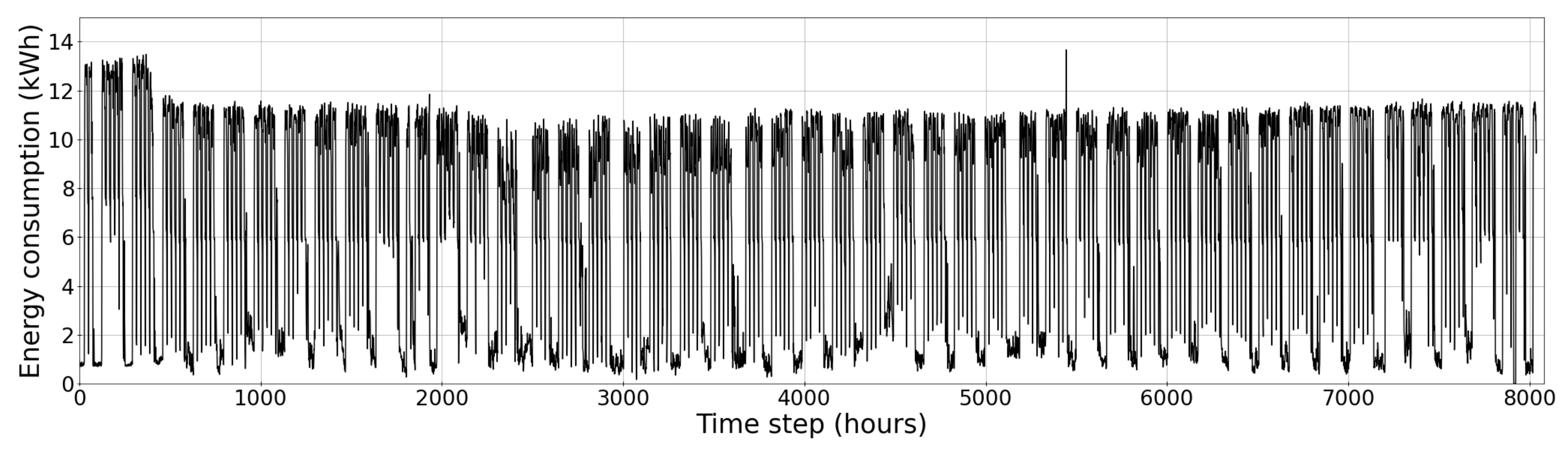
2.1. Dataset
2.2. Data Preprocessing
2.3. Evaluation Metric
3. Model Identification
3.1. Machine Learning Models
3.2. Deep Learning Models
3.3. Benchmarks
4. Discussion
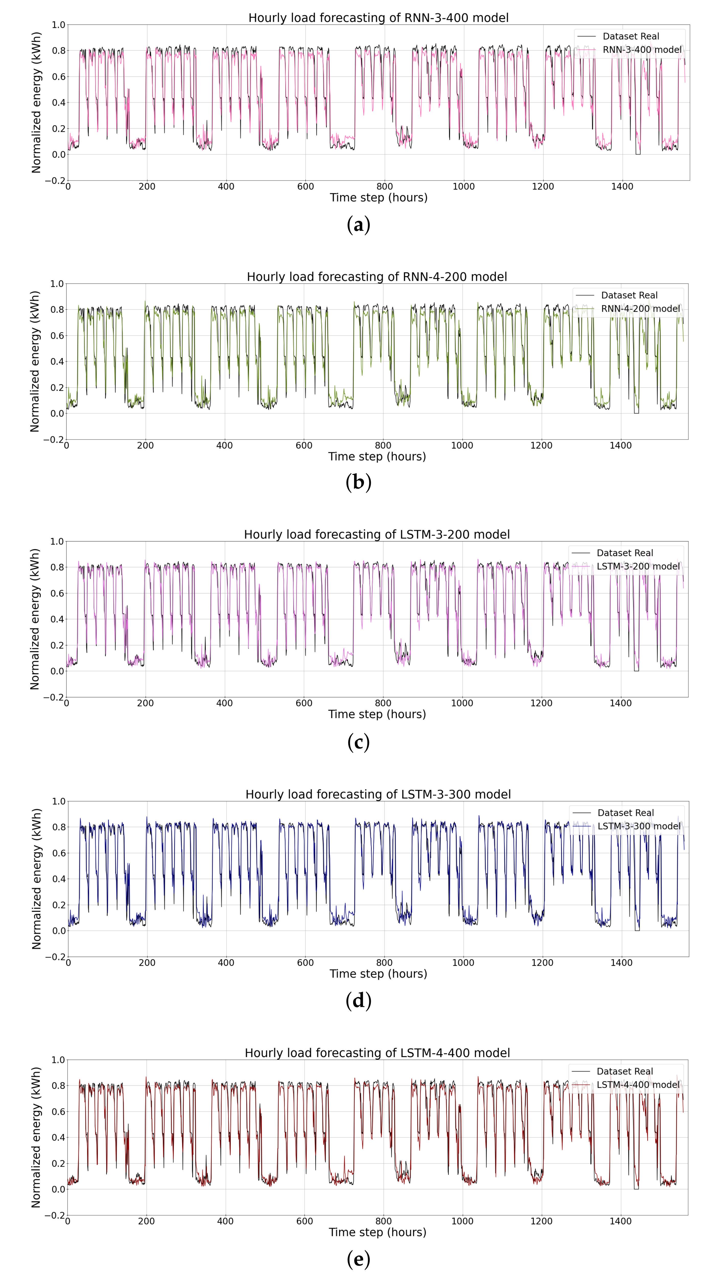
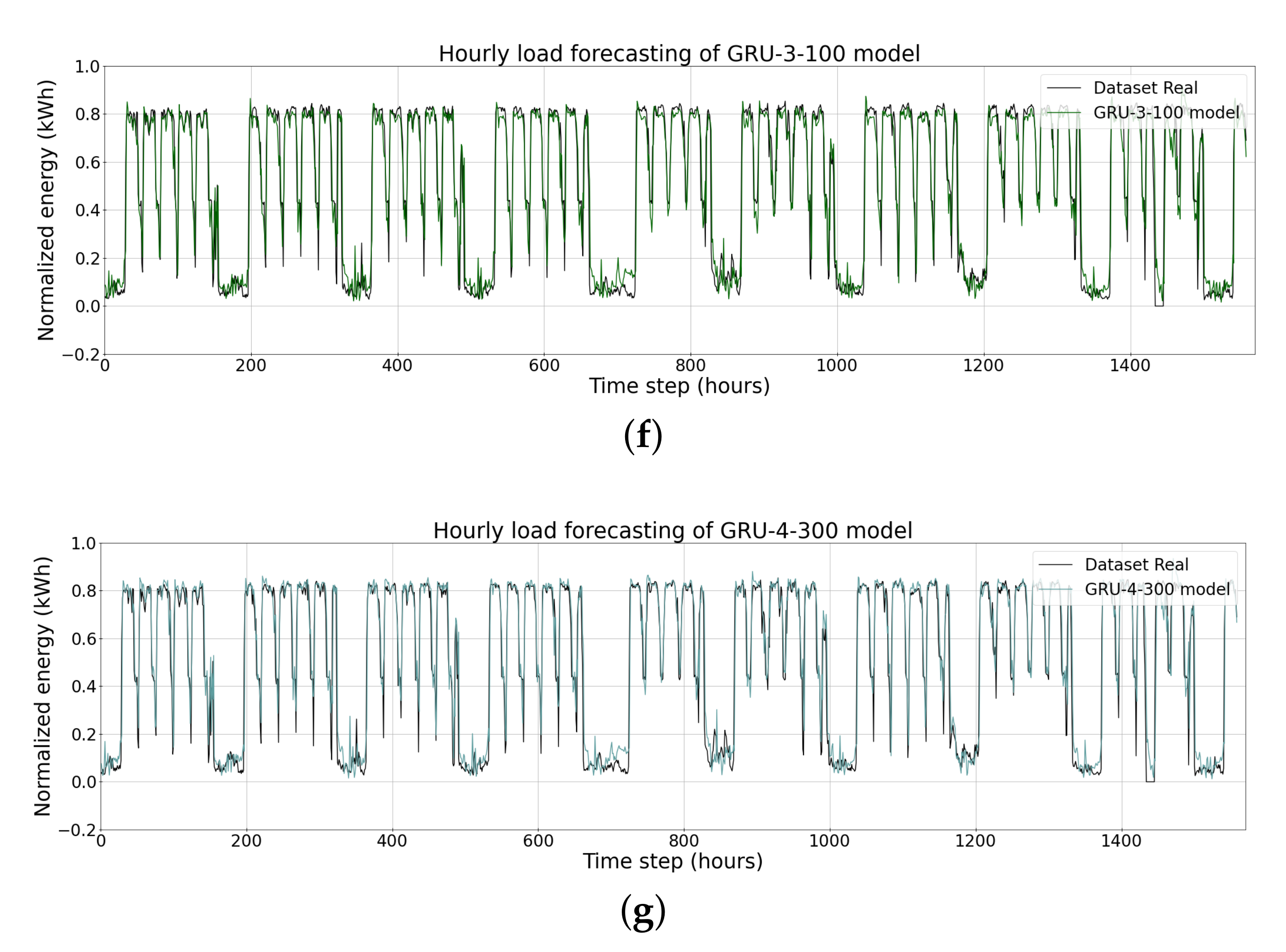
4.1. Short-Term Load Forecasting
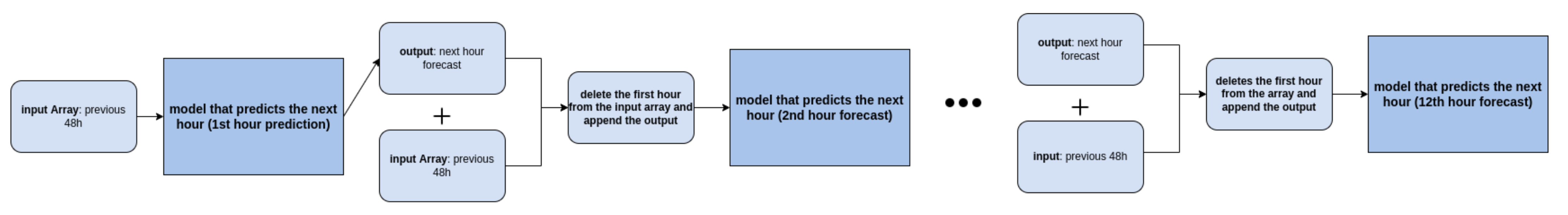
4.2. Very Short-Term Load Forecasting
5. Related Work
6. Conclusions and Future Work
Author Contributions
Funding
Institutional Review Board Statement
Informed Consent Statement
Data Availability Statement
Acknowledgments
Conflicts of Interest
Abbreviations
| ANN | Artificial Neural Networks |
| AMI | Advanced Metering Infrastructure |
| ANN | Artificial Neural Network |
| ARIMA | Autoregressive Integrated Moving Average |
| CV | Co-efficient of Variance |
| EPC | Energy Performance Contract |
| ESCO | Energy Service Company |
| EU | European Union |
| GB | Gradient Boosting |
| GHG | Greenhouse Gas |
| GRU | Gated Recurrent Unit |
| HVAC | Heating, Ventilation and Air Conditioning |
| LED | Light Emitting Diode |
| LSTM | Long Short-Term Memory |
| MAE | Mean Absolute Error |
| MLR | Multiple Linear Regression |
| MAPE | Mean Absolute Percent Error |
| MSE | Mean Squared Error |
| PV | Solar Photovoltaic |
| RF | Random Forest |
| RMSE | Root Mean Squared Error |
| RNN | Recurrent Neural Networks |
| STLF | Short-Term Load Forecasting |
| SVM | Support Vector Machines |
| SVR | Support Vector Machine Regression |
| UN | United Nations |
| VSTLF | Very Short-Term Load Forecasting |
| XGBoost | Extreme Gradient Boosting |
References
- Bové, A.T.; Swartz, S. Starting at the Source: Sustainability in Supply Chains. 2016. Available online: https://www.mckinsey.com/business-functions/sustainability/our-insights/starting-at-the-source-sustainability-in-supply-chains (accessed on 10 November 2021).
- Rakhmangulov, A.; Sladkowski, A.; Osintsev, N.; Muravev, D. Green Logistics: A System of Methods and Instruments-Part 2. NAŠE MORE Znanstveni Časopis za More i Pomorstvo 2018, 65, 49–55. [Google Scholar] [CrossRef] [Green Version]
- Smokers, R.; Tavasszy, L.; Chen, M.; Guis, E. Options for Competitive and Sustainable Logistics; Emerald Group Publishing Limited: Bingley, UK, 2014. [Google Scholar]
- Depreaux, J. 28,500 Warehouses To Be Added Globally To Meet E-Commerce Boom. 2021. Available online: https://www.interactanalysis.com/28500-warehouses-to-be-added-globally-to-meet-e-commerce-boom/ (accessed on 13 December 2021).
- Trust, C. Warehousing and Logistics—Energy Opportunities for Warehousing and Logistics Companies. 2019. Available online: https://www.carbontrust.com/resources/warehousing-and-logistics-guide (accessed on 13 December 2021).
- Lewczuk, K.; Kłodawski, M.; Gepner, P. Energy Consumption in a Distributional Warehouse: A Practical Case Study for Different Warehouse Technologies. Energies 2021, 14, 2709. [Google Scholar] [CrossRef]
- World Economic Forum; Accenture. Supply Chain Decarbonisation: The Role of Logistics and Transport in Reducing Supply Chain Carbon Emissions; World Economic Forum and Accenture Geneva: Geneva, Switzerland, 2009. [Google Scholar]
- Dagdougui, H.; Bagheri, F.; Le, H.; Dessaint, L. Neural network model for short-term and very-short-term load forecasting in district buildings. Energy Build. 2019, 203, 109408. [Google Scholar] [CrossRef]
- Chitalia, G.; Pipattanasomporn, M.; Garg, V.; Rahman, S. Robust short-term electrical load forecasting framework for commercial buildings using deep recurrent neural networks. Appl. Energy 2020, 278, 115410. [Google Scholar] [CrossRef]
- Hippert, H.S.; Pedreira, C.E.; Souza, R.C. Neural networks for short-term load forecasting: A review and evaluation. IEEE Trans. Power Syst. 2001, 16, 44–55. [Google Scholar] [CrossRef]
- Ribeiro, A.M.N.; do Carmo, P.R.X.; Rodrigues, I.R.; Sadok, D.; Lynn, T.; Endo, P.T. Short-Term Firm-Level Energy-Consumption Forecasting for Energy-Intensive Manufacturing: A Comparison of Machine Learning and Deep Learning Models. Algorithms 2020, 13, 274. [Google Scholar] [CrossRef]
- Quilumba, F.L.; Lee, W.J.; Huang, H.; Wang, D.Y.; Szabados, R.L. Using smart meter data to improve the accuracy of intraday load forecasting considering customer behavior similarities. IEEE Trans. Smart Grid 2014, 6, 911–918. [Google Scholar] [CrossRef]
- Alahmad, M.; Peng, Y.; Sordiashie, E.; El Chaar, L.; Aljuhaishi, N.; Sharif, H. Information technology and the smart grid-A pathway to conserve energy in buildings. In Proceedings of the 2013 9th International Conference on Innovations in Information Technology (IIT), Abu Dhabi, United Arab Emirates, 17–19 March 2013; pp. 60–65. [Google Scholar]
- Bertoldi, P.; Boza-Kiss, B.; Toleikyté, A. Energy Service Market in the EU; Publications Office of the European Union: Luxembourg, 2019. [Google Scholar]
- European Commission. A Renovation Wave for Europe—Greening Our Buildings, Creating Jobs, Improving Lives. 2020. Available online: https://ec.europa.eu/energy/sites/ener/files/eu_renovation_wave_strategy.pdf (accessed on 12 April 2021).
- Sorrell, S. The economics of energy service contracts. Energy Policy 2007, 35, 507–521. [Google Scholar] [CrossRef]
- Fallah, S.N.; Ganjkhani, M.; Shamshirband, S.; Chau, K.W. Computational intelligence on short-term load forecasting: A methodological overview. Energies 2019, 12, 393. [Google Scholar] [CrossRef] [Green Version]
- Raza, M.Q.; Khosravi, A. A review on artificial intelligence based load demand forecasting techniques for smart grid and buildings. Renew. Sustain. Energy Rev. 2015, 50, 1352–1372. [Google Scholar] [CrossRef]
- Daut, M.A.M.; Hassan, M.Y.; Abdullah, H.; Rahman, H.A.; Abdullah, M.P.; Hussin, F. Building electrical energy consumption forecasting analysis using conventional and artificial intelligence methods: A review. Renew. Sustain. Energy Rev. 2017, 70, 1108–1118. [Google Scholar] [CrossRef]
- Sola, J.; Sevilla, J. Importance of input data normalization for the application of neural networks to complex industrial problems. IEEE Trans. Nucl. Sci. 1997, 44, 1464–1468. [Google Scholar] [CrossRef]
- Debnath, K.B.; Mourshed, M. Forecasting methods in energy planning models. Renew. Sustain. Energy Rev. 2018, 88, 297–325. [Google Scholar] [CrossRef] [Green Version]
- Willmott, C.J.; Matsuura, K. Advantages of the mean absolute error (MAE) over the root mean square error (RMSE) in assessing average model performance. Clim. Res. 2005, 30, 79–82. [Google Scholar] [CrossRef]
- Kolomvatsos, K.; Papadopoulou, P.; Anagnostopoulos, C.; Hadjiefthymiades, S. Anagnostopoulos, C.; Hadjiefthymiades, S. A Spatio-Temporal Data Imputation Model for Supporting Analytics at the Edge. In Conference on e-Business, e-Services and e-Society; Springer: Berlin/Heidelberg, Germany, 2019; pp. 138–150. [Google Scholar]
- Luo, J.; Hong, T.; Yue, M. Real-time anomaly detection for very short-term load forecasting. J. Mod. Power Syst. Clean Energy 2018, 6, 235–243. [Google Scholar] [CrossRef] [Green Version]
- Ryu, S.; Noh, J.; Kim, H. Deep neural network based demand side short term load forecasting. Energies 2017, 10, 3. [Google Scholar] [CrossRef]
- Berriel, R.F.; Lopes, A.T.; Rodrigues, A.; Varejao, F.M.; Oliveira-Santos, T. Monthly energy consumption forecast: A deep learning approach. In Proceedings of the 2017 International Joint Conference on Neural Networks (IJCNN), Anchorage, AK, USA, 14–19 May 2017; pp. 4283–4290. [Google Scholar]
- Azadeh, A.; Ghaderi, S.; Sohrabkhani, S. Annual electricity consumption forecasting by neural network in high energy consuming industrial sectors. Energy Convers. Manag. 2008, 49, 2272–2278. [Google Scholar] [CrossRef]
- Kuo, P.H.; Huang, C.J. A high precision artificial neural networks model for short-term energy load forecasting. Energies 2018, 11, 213. [Google Scholar] [CrossRef] [Green Version]
- Kong, W.; Dong, Z.Y.; Jia, Y.; Hill, D.J.; Xu, Y.; Zhang, Y. Short-term residential load forecasting based on LSTM recurrent neural network. IEEE Trans. Smart Grid 2017, 10, 841–851. [Google Scholar] [CrossRef]
- De Myttenaere, A.; Golden, B.; Le Grand, B.; Rossi, F. Mean absolute percentage error for regression models. Neurocomputing 2016, 192, 38–48. [Google Scholar] [CrossRef] [Green Version]
- Hsieh, T.J.; Hsiao, H.F.; Yeh, W.C. Forecasting stock markets using wavelet transforms and recurrent neural networks: An integrated system based on artificial bee colony algorithm. Appl. Soft Comput. 2011, 11, 2510–2525. [Google Scholar] [CrossRef]
- Chen, C.; Liu, Y.; Kumar, M.; Qin, J. Energy consumption modelling using deep learning technique—A case study of EAF. Procedia CIRP 2018, 72, 1063–1068. [Google Scholar] [CrossRef]
- Li, C.; Tao, Y.; Ao, W.; Yang, S.; Bai, Y. Improving forecasting accuracy of daily enterprise electricity consumption using a random forest based on ensemble empirical mode decomposition. Energy 2018, 165, 1220–1227. [Google Scholar] [CrossRef]
- Chae, Y.T.; Horesh, R.; Hwang, Y.; Lee, Y.M. Artificial neural network model for forecasting sub-hourly electricity usage in commercial buildings. Energy Build. 2016, 111, 184–194. [Google Scholar] [CrossRef]
- Chen, J.F.; Wang, W.M.; Huang, C.M. Analysis of an adaptive time-series autoregressive moving-average (ARMA) model for short-term load forecasting. Electr. Power Syst. Res. 1995, 34, 187–196. [Google Scholar] [CrossRef]
- Huang, S.J.; Shih, K.R. Short-term load forecasting via ARMA model identification including non-Gaussian process considerations. IEEE Trans. Power Syst. 2003, 18, 673–679. [Google Scholar] [CrossRef] [Green Version]
- Kim, Y.; Son, H.g.; Kim, S. Short term electricity load forecasting for institutional buildings. Energy Rep. 2019, 5, 1270–1280. [Google Scholar] [CrossRef]
- Huang, C.M.; Huang, C.J.; Wang, M.L. A particle swarm optimization to identifying the ARMAX model for short-term load forecasting. IEEE Trans. Power Syst. 2005, 20, 1126–1133. [Google Scholar] [CrossRef]
- Chakhchoukh, Y.; Panciatici, P.; Mili, L. Electric load forecasting based on statistical robust methods. IEEE Trans. Power Syst. 2010, 26, 982–991. [Google Scholar] [CrossRef]
- Yang, J.; Stenzel, J. Short-term load forecasting with increment regression tree. Electr. Power Syst. Res. 2006, 76, 880–888. [Google Scholar] [CrossRef]
- Ceperic, E.; Ceperic, V.; Baric, A. A strategy for short-term load forecasting by support vector regression machines. IEEE Trans. Power Syst. 2013, 28, 4356–4364. [Google Scholar] [CrossRef]
- Chen, Y.; Tan, H. Short-term prediction of electric demand in building sector via hybrid support vector regression. Appl. Energy 2017, 204, 1363–1374. [Google Scholar] [CrossRef]
- Chen, Y.; Xu, P.; Chu, Y.; Li, W.; Wu, Y.; Ni, L.; Bao, Y.; Wang, K. Short-term electrical load forecasting using the Support Vector Regression (SVR) model to calculate the demand response baseline for office buildings. Appl. Energy 2017, 195, 659–670. [Google Scholar] [CrossRef]
- Li, Q.; Zhang, L.; Xiang, F. Short-term load forecasting: A case study in Chongqing factories. In Proceedings of the 2019 6th International Conference on Information Science and Control Engineering (ICISCE), Shanghai, China, 20–22 December 2019; pp. 892–897. [Google Scholar]
- Zhu, K.; Geng, J.; Wang, K. A hybrid prediction model based on pattern sequence-based matching method and extreme gradient boosting for holiday load forecasting. Electr. Power Syst. Res. 2021, 190, 106841. [Google Scholar] [CrossRef]
- Zheng, H.; Yuan, J.; Chen, L. Short-term load forecasting using EMD-LSTM neural networks with a Xgboost algorithm for feature importance evaluation. Energies 2017, 10, 1168. [Google Scholar] [CrossRef] [Green Version]
- Grolinger, K.; L’Heureux, A.; Capretz, M.A.; Seewald, L. Energy forecasting for event venues: Big data and prediction accuracy. Energy Build. 2016, 112, 222–233. [Google Scholar] [CrossRef] [Green Version]
- Singh, S.; Hussain, S.; Bazaz, M.A. Short term load forecasting using artificial neural network. In Proceedings of the 2017 Fourth International Conference on Image Information Processing (ICIIP), Shimla, India, 21–23 December 2017; pp. 1–5. [Google Scholar]
- Huang, Q.; Li, J.; Zhu, M. An improved convolutional neural network with load range discretization for probabilistic load forecasting. Energy 2020, 203, 117902. [Google Scholar] [CrossRef]
- Bengio, Y.; Simard, P.; Frasconi, P. Learning long-term dependencies with gradient descent is difficult. IEEE Trans. Neural Netw. 1994, 5, 157–166. [Google Scholar] [CrossRef]
- Pascanu, R.; Mikolov, T.; Bengio, Y. On the difficulty of training recurrent neural networks. Int. Conf. Mach. Learn. PMLR 2013, 28, 1310–1318. [Google Scholar]
- Sundermeyer, M.; Schlüter, R.; Ney, H. LSTM neural networks for language modeling. In Proceedings of the Thirteenth Annual Conference of the International Speech Communication Association, Portland, OR, USA, 9–13 September 2012. [Google Scholar]
- Marino, D.L.; Amarasinghe, K.; Manic, M. Building energy load forecasting using deep neural networks. In Proceedings of the IECON 2016-42nd Annual Conference of the IEEE Industrial Electronics Society, Florence, Italy, 24–27 October 2016; pp. 7046–7051. [Google Scholar]
- Kuan, L.; Yan, Z.; Xin, W.; Yan, C.; Xiangkun, P.; Wenxue, S.; Zhe, J.; Yong, Z.; Nan, X.; Xin, Z. Short-term electricity load forecasting method based on multilayered self-normalizing GRU network. In Proceedings of the 2017 IEEE Conference on Energy Internet and Energy System Integration (EI2), Beijing, China, 26–28 November 2017; pp. 1–5. [Google Scholar]
- He, F.; Zhou, J.; Feng, Z.k.; Liu, G.; Yang, Y. A hybrid short-term load forecasting model based on variational mode decomposition and long short-term memory networks considering relevant factors with Bayesian optimization algorithm. Appl. Energy 2019, 237, 103–116. [Google Scholar] [CrossRef]
- Chung, J.; Gulcehre, C.; Cho, K.; Bengio, Y. Empirical evaluation of gated recurrent neural networks on sequence modeling. arXiv 2014, arXiv:1412.3555. [Google Scholar]
- Wang, Y.; Liu, M.; Bao, Z.; Zhang, S. Short-term load forecasting with multi-source data using gated recurrent unit neural networks. Energies 2018, 11, 1138. [Google Scholar] [CrossRef] [Green Version]
- Wu, W.; Liao, W.; Miao, J.; Du, G. Using gated recurrent unit network to forecast short-term load considering impact of electricity price. Energy Procedia 2019, 158, 3369–3374. [Google Scholar] [CrossRef]
- Drucker, H.; Burges, C.J.; Kaufman, L.; Smola, A.; Vapnik, V. Support vector regression machines. Adv. Neural Inf. Process. Syst. 1997, 9, 155–161. [Google Scholar]
- Vapnik, V. The Nature of Statistical Learning Theory; Springer: New York, NY, USA, 1995; Volume 10, p. 189. 978p. [Google Scholar]
- Sapankevych, N.I.; Sankar, R. Time series prediction using support vector machines: A survey. IEEE Comput. Intell. Mag. 2009, 4, 24–38. [Google Scholar] [CrossRef]
- Breiman, L. Random forests. Mach. Learn. 2001, 45, 5–32. [Google Scholar] [CrossRef] [Green Version]
- Huang, N.; Lu, G.; Xu, D. A permutation importance-based feature selection method for short-term electricity load forecasting using random forest. Energies 2016, 9, 767. [Google Scholar] [CrossRef] [Green Version]
- Breiman, L. Bagging predictors. Mach. Learn. 1996, 24, 123–140. [Google Scholar] [CrossRef] [Green Version]
- Ho, T.K. The random subspace method for constructing decision forests. IEEE Trans. Pattern Anal. Mach. Intell. 1998, 20, 832–844. [Google Scholar]
- Nadi, A.; Moradi, H. Increasing the views and reducing the depth in random forest. Expert Syst. Appl. 2019, 138, 112801. [Google Scholar] [CrossRef]
- Hammou, B.A.; Lahcen, A.A.; Mouline, S. An effective distributed predictive model with Matrix factorization and random forest for Big Data recommendation systems. Expert Syst. Appl. 2019, 137, 253–265. [Google Scholar] [CrossRef]
- Wang, Y.; Sun, S.; Chen, X.; Zeng, X.; Kong, Y.; Chen, J.; Guo, Y.; Wang, T. Short-term load forecasting of industrial customers based on SVMD and XGBoost. Int. J. Electr. Power Energy Syst. 2021, 129, 106830. [Google Scholar] [CrossRef]
- Zhang, B.; Wu, J.L.; Chang, P.C. A multiple time series-based recurrent neural network for short-term load forecasting. Soft Comput. 2018, 22, 4099–4112. [Google Scholar] [CrossRef]
- Gers, F.A.; Schmidhuber, J.; Cummins, F. Learning to forget: Continual prediction with LSTM. In Proceedings of the 1999 Ninth International Conference on Artificial Neural Networks ICANN 99 (Conf. Publ. No. 470), Edinburgh, UK, 7–10 September 1999; Volume 2, pp. 850–855. [Google Scholar] [CrossRef]
- Hochreiter, S.; Schmidhuber, J. Long short-term memory. Neural Comput. 1997, 9, 1735–1780. [Google Scholar] [CrossRef]
- Jozefowicz, R.; Zaremba, W.; Sutskever, I. An empirical exploration of recurrent network architectures. Int. Conf. Mach. Learn. 2015, 37, 2342–2350. [Google Scholar]
- Yu, Y.; Si, X.; Hu, C.; Zhang, J. A review of recurrent neural networks: LSTM cells and network architectures. Neural Comput. 2019, 31, 1235–1270. [Google Scholar] [CrossRef]
- Bergstra, J.; Bengio, Y. Random search for hyper-parameter optimization. J. Mach. Learn. Res. 2012, 13, 281–305. [Google Scholar]
- Liao, J.M.; Chang, M.J.; Chang, L.M. Prediction of Air-Conditioning Energy Consumption in R&D Building Using Multiple Machine Learning Techniques. Energies 2020, 13, 1847. [Google Scholar]
- Yoon, H.; Kim, Y.; Ha, K.; Lee, S.H.; Kim, G.P. Comparative evaluation of ANN-and SVM-time series models for predicting freshwater-saltwater interface fluctuations. Water 2017, 9, 323. [Google Scholar] [CrossRef] [Green Version]
- Kavaklioglu, K. Modeling and prediction of Turkey’s electricity consumption using Support Vector Regression. Appl. Energy 2011, 88, 368–375. [Google Scholar] [CrossRef]
- Samsudin, R.; Shabri, A.; Saad, P. A comparison of time series forecasting using support vector machine and artificial neural network model. J. Appl. Sci. 2010, 10, 950–958. [Google Scholar] [CrossRef] [Green Version]
- Han, J.; Moraga, C. The influence of the sigmoid function parameters on the speed of backpropagation learning. In From Natural to Artificial Neural Computation; Mira, J., Sandoval, F., Eds.; Springer: Berlin/Heidelberg, Germany, 1995; pp. 195–201. [Google Scholar]
- Vaghefi, A.; Jafari, M.A.; Bisse, E.; Lu, Y.; Brouwer, J. Modeling and forecasting of cooling and electricity load demand. Appl. Energy 2014, 136, 186–196. [Google Scholar] [CrossRef] [Green Version]
- Pushp, S. Merging Two Arima Models for Energy Optimization in WSN. arXiv 2010, arXiv:1006.5436. [Google Scholar]
- Hsiao, Y.H. Household electricity demand forecast based on context information and user daily schedule analysis from meter data. IEEE Trans. Ind. Inform. 2014, 11, 33–43. [Google Scholar] [CrossRef]
- Mele, E. A review of machine learning algorithms used for load forecasting at microgrid level. In Sinteza 2019-International Scientific Conference on Information Technology and Data Related Research; Singidunum University: Beograd, Serbia, 2019; pp. 452–458. [Google Scholar]
- Shwartz-Ziv, R.; Armon, A. Tabular data: Deep learning is not all you need. Inf. Fusion 2022, 81, 84–90. [Google Scholar] [CrossRef]
- Gassar, A.A.A.; Cha, S.H. Energy prediction techniques for large-scale buildings towards a sustainable built environment: A review. Energy Build. 2020, 224, 110238. [Google Scholar] [CrossRef]
- Charytoniuk, W.; Chen, M.S. Very short-term load forecasting using artificial neural networks. IEEE Trans. Power Syst. 2000, 15, 263–268. [Google Scholar] [CrossRef]
- Guan, C.; Luh, P.B.; Michel, L.D.; Wang, Y.; Friedland, P.B. Very short-term load forecasting: Wavelet neural networks with data pre-filtering. IEEE Trans. Power Syst. 2012, 28, 30–41. [Google Scholar] [CrossRef]
- Li, G.; Zhao, X.; Fan, C.; Fang, X.; Li, F.; Wu, Y. Assessment of long short-term memory and its modifications for enhanced short-term building energy predictions. J. Build. Eng. 2021, 43, 103182. [Google Scholar] [CrossRef]
- Escrivá-Escrivá, G.; Álvarez-Bel, C.; Roldán-Blay, C.; Alcázar-Ortega, M. New artificial neural network prediction method for electrical consumption forecasting based on building end-uses. Energy Build. 2011, 43, 3112–3119. [Google Scholar] [CrossRef]
- Neto, A.H.; Fiorelli, F.A.S. Comparison between detailed model simulation and artificial neural network for forecasting building energy consumption. Energy Build. 2008, 40, 2169–2176. [Google Scholar] [CrossRef]
- Gonzalez, P.A.; Zamarreno, J.M. Prediction of hourly energy consumption in buildings based on a feedback artificial neural network. Energy Build. 2005, 37, 595–601. [Google Scholar] [CrossRef]
- Zajac, P. Evaluation Method of Energy Consumption in Logistic Warehouse Systems; Springer: Berlin/Heidelberg, Germany, 2015. [Google Scholar]
- Rüdiger, D.; Schön, A.; Dobers, K. Managing greenhouse gas emissions from warehousing and transshipment with environmental performance indicators. Transp. Res. Procedia 2016, 14, 886–895. [Google Scholar] [CrossRef]


| Quantile Statistics | Descriptive Statistics | ||
|---|---|---|---|
| Description | Values | Description | Values |
| Minimum | 0.00 | Standard deviation | 4.18 |
| Maximum | 13.67 | Coefficient of variation | 0.63 |
| Median | 7.69 | Mean | 6.68 |
| Range | 13.67 | Median Absoluta Deviation | 3.26 |
| Interquartile range | 9.02 | Variance | 17.44 |
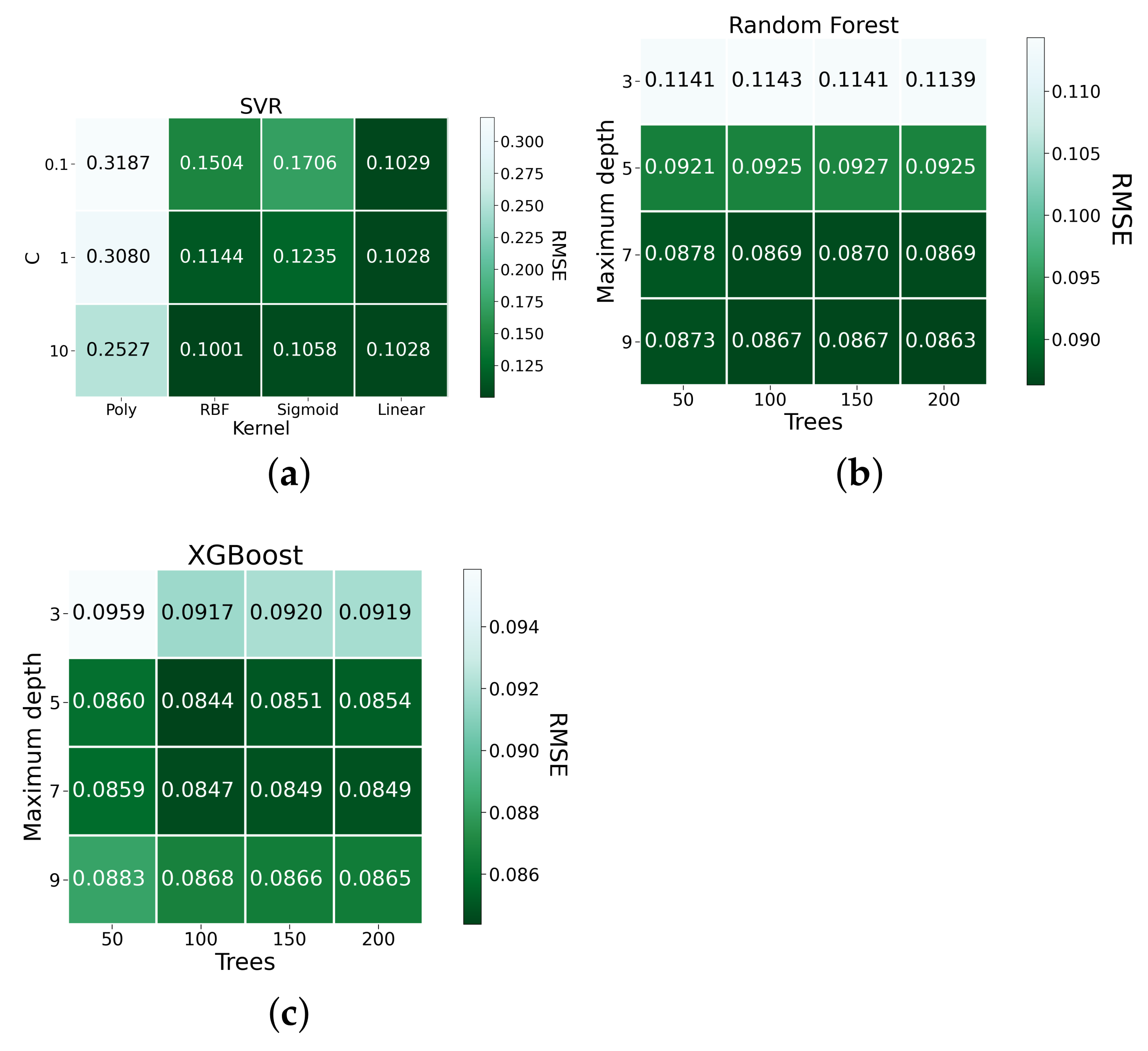
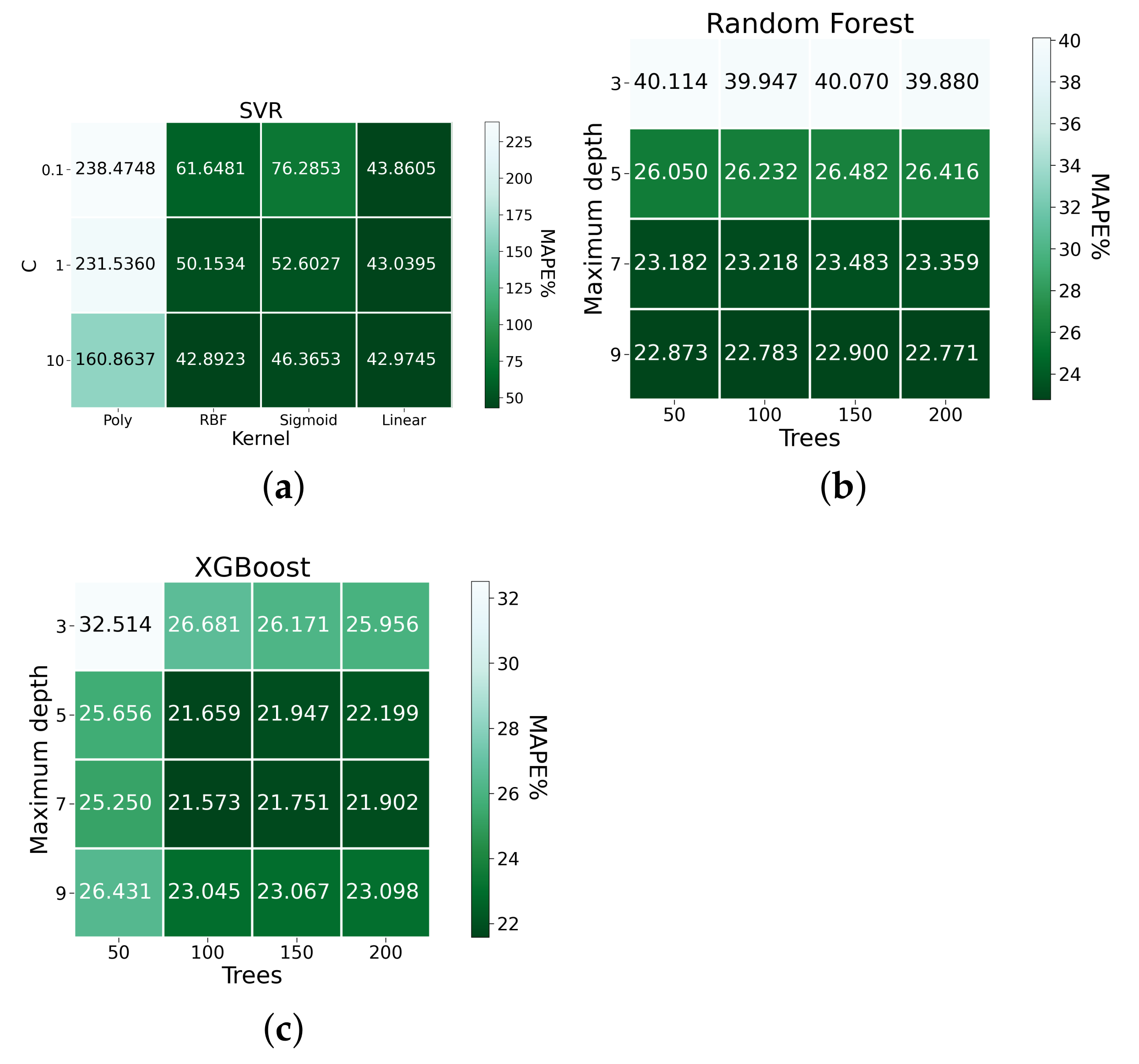
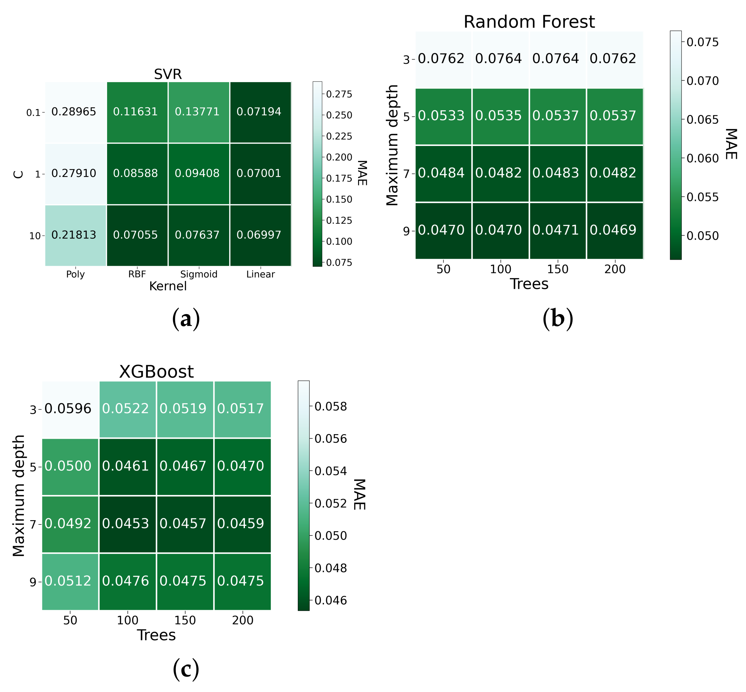
| Technique | Parameter | Levels |
|---|---|---|
| SVR | Number of C | 0.1, 1, and 10 |
| SVR | Type of kernel | Polinomial, RBF, sigmoid, and linear |
| Random Forest | Number of max. depth | From 3 to 9, step 2 |
| Random Forest | Number of trees | From 50 to 200, step 50 |
| XGBoost | Number of max. depth | From 3 to 9, step 2 |
| XGBoost | Number of trees | From 50 to 200, step 50 |
| Parameter | Levels |
|---|---|
| Number of nodes | From 100 to 400, step 100 |
| Number of layers | From 1 to 4, step 1 |
| Model Parameters | |||
|---|---|---|---|
| Layer Number | Layers | Repetitions of Layer | NUM_UNITS |
| 1 | LSTM, GRU or RNN | 1, 2, 3 or 4 | 100, 200, 300 or 400 |
| 2 | Dense (1, activation = adam) | - | - |
| Compile Parameters | |||
| Loss function | MSE | ||
| Optimiser | ADAM | ||
| Early stoppin | EarlyStopping (monitor = ’val_loss’, mode = ’auto’, verbose = 1, min_delta = 0.001, patience = 10) | ||
| Batch size | 256 | ||
| Epochs | 1000 | ||
| Models | RMSE | MAPE (%) | MAE |
|---|---|---|---|
| ARIMA | 0.1114 | 28.8016 | 0.0615 |
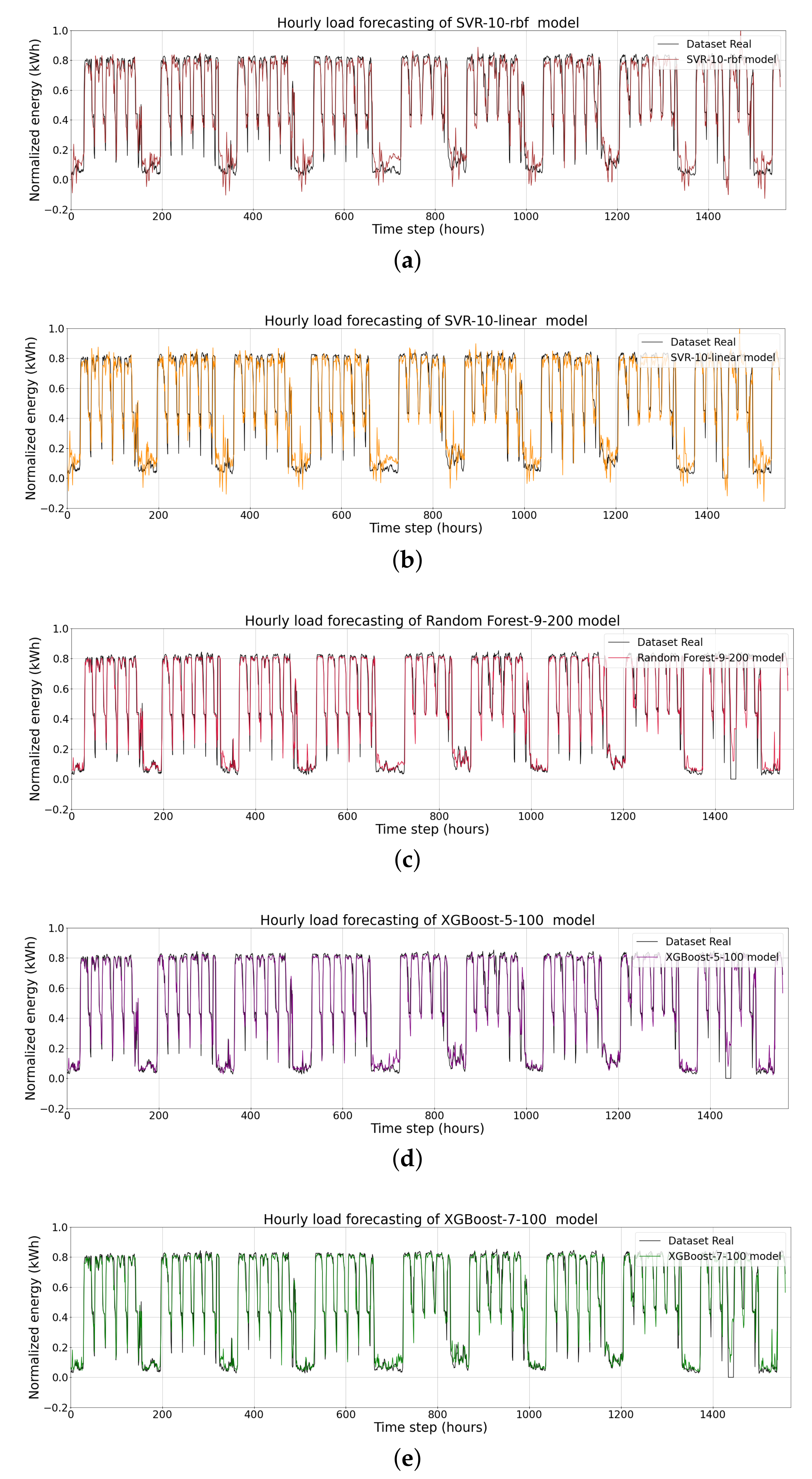
| SVR-10-rbf | 0.1001 | 42.8923 | 0.0705 |
| SVR-10-linear | 0.1028 | 42.9745 | 0.0610 |
| Random Forest-9-200 | 0.0863 | 22.771 | 0.0469 |
| XGBoost-5-100 | 0.0844 | 21.659 | 0.0461 |
| XGBoost-7-100 | 0.0847 | 21.573 | 0.0453 |
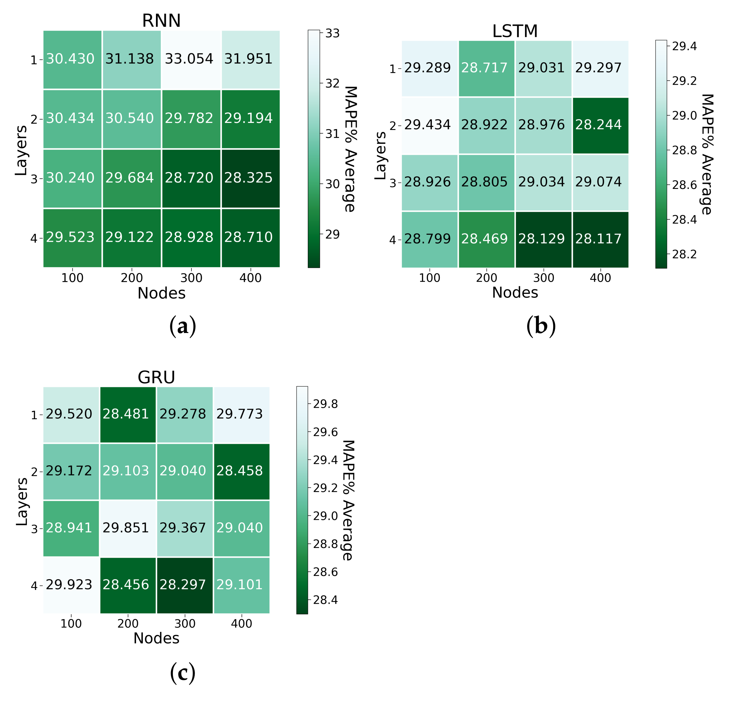
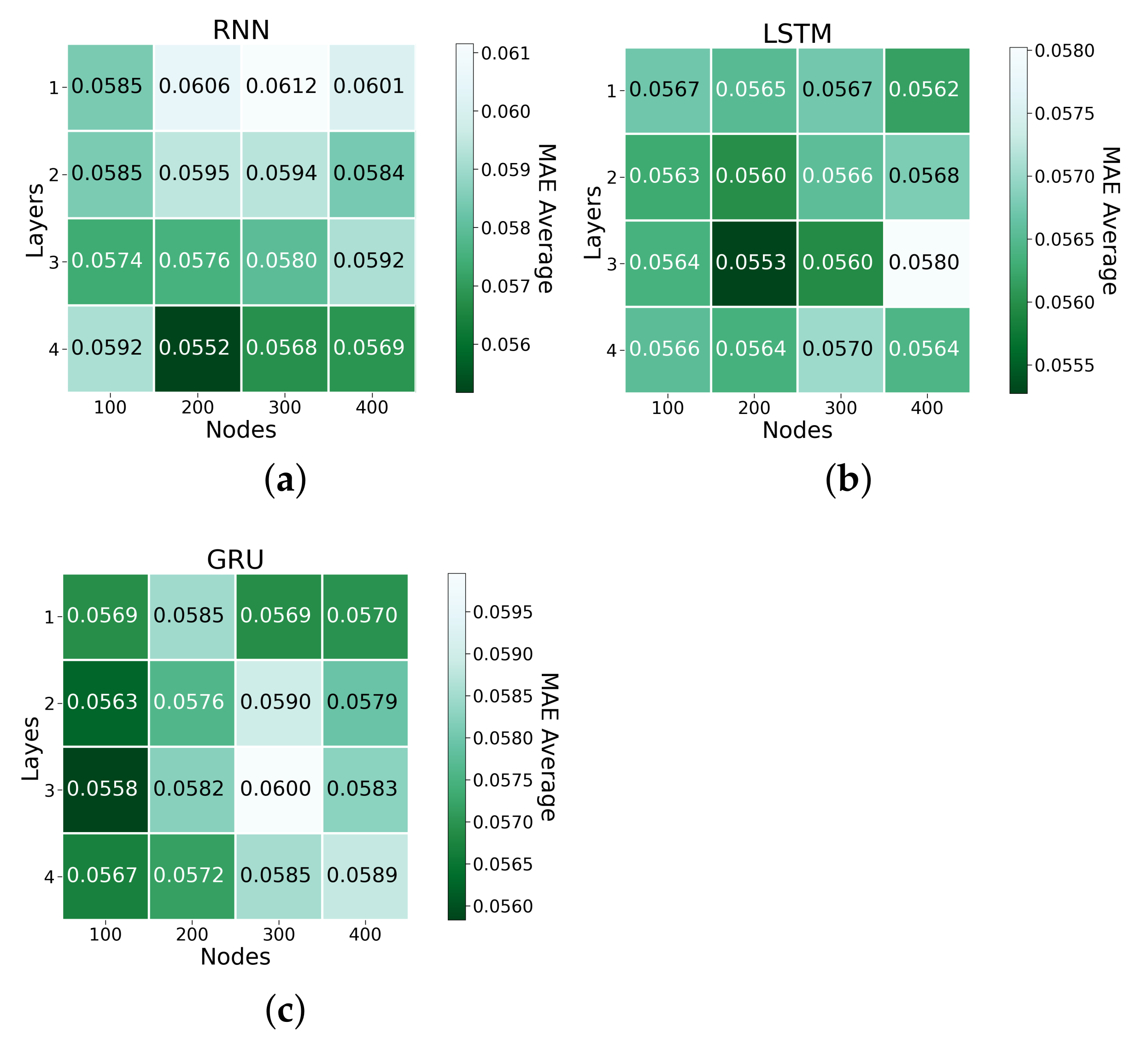
| RNN-3-400 | 0.0947 | 28.325 | 0.0592 |
| RNN-4-200 | 0.0909 | 29.122 | 0.0552 |
| LSTM-3-200 | 0.0912 | 28.805 | 0.0553 |
| LSTM-3-300 | 0.0911 | 29.03 | 0.0560 |
| LSTM-4-400 | 0.0919 | 28.117 | 0.0564 |
| GRU-3-100 | 0.0918 | 28.94 | 0.0558 |
| GRU-4-300 | 0.0933 | 28.297 | 0.0585 |
| Models | Prediction (h) | RMSE | MAPE (%) | MAE |
|---|---|---|---|---|
| XGBoost-5-100 | 1 | 0.0844 | 21.659 | 0.0461 |
| XGBoost-7-100 | 1 | 0.0847 | 21.573 | 0.0453 |
| XGBoost-5-100 | 12 | 0.1835 | 21.580 | 0.1009 |
| XGBoost-7-100 | 12 | 0.1717 | 21.749 | 0.0926 |
| XGBoost-5-100 | 24 | 0.2342 | 21.603 | 0.1370 |
| XGBoost-7-100 | 24 | 0.2149 | 21.639 | 0.1232 |
Publisher’s Note: MDPI stays neutral with regard to jurisdictional claims in published maps and institutional affiliations. |
© 2022 by the authors. Licensee MDPI, Basel, Switzerland. This article is an open access article distributed under the terms and conditions of the Creative Commons Attribution (CC BY) license (https://creativecommons.org/licenses/by/4.0/).
Share and Cite
Ribeiro, A.M.N.C.; do Carmo, P.R.X.; Endo, P.T.; Rosati, P.; Lynn, T. Short- and Very Short-Term Firm-Level Load Forecasting for Warehouses: A Comparison of Machine Learning and Deep Learning Models. Energies 2022, 15, 750. https://0-doi-org.brum.beds.ac.uk/10.3390/en15030750
Ribeiro AMNC, do Carmo PRX, Endo PT, Rosati P, Lynn T. Short- and Very Short-Term Firm-Level Load Forecasting for Warehouses: A Comparison of Machine Learning and Deep Learning Models. Energies. 2022; 15(3):750. https://0-doi-org.brum.beds.ac.uk/10.3390/en15030750
Chicago/Turabian StyleRibeiro, Andrea Maria N. C., Pedro Rafael X. do Carmo, Patricia Takako Endo, Pierangelo Rosati, and Theo Lynn. 2022. "Short- and Very Short-Term Firm-Level Load Forecasting for Warehouses: A Comparison of Machine Learning and Deep Learning Models" Energies 15, no. 3: 750. https://0-doi-org.brum.beds.ac.uk/10.3390/en15030750