
Artificial Intelligence Applications in Estimating Invisible Solar Power Generation


1
Department of Electrical Engineering, National Chung-Cheng University, Chia-Yi 62102, Taiwan
2
School of Engineering and Advance Engineering Platform, Monash University Malaysia, Subang Jaya 47500, Selangor, Malaysia
*
Author to whom correspondence should be addressed.
Energies 2022, 15(4), 1312; https://0-doi-org.brum.beds.ac.uk/10.3390/en15041312
Submission received: 31 December 2021
/
Revised: 5 February 2022
/
Accepted: 8 February 2022
/
Published: 11 February 2022
(This article belongs to the Special Issue Artificial Intelligence (AI) in the Power Grid and Renewable Energy)
Abstract
:In recent years, the penetration of photovoltaic (PV) power generation in Taiwan has increased significantly. However, most photovoltaic facilities, especially for small-scale sites, do not include relevant monitoring and real-time measurement devices. The invisible power generation from these PV sites would cause a huge challenge on power system scheduling. Therefore, appropriate methods to estimate invisible PV power generation are needed. The main purpose of this paper is to propose an improved fuzzy model for estimating the PV power generation, which includes the clustering processing for PV sites, selection of representative PV sites, and the improvement of the conventional fuzzy model. First, this research uses the K-nearest neighbor (KNN) algorithm to fill in some of the missing data; then, two clustering algorithms are applied to cluster all the photovoltaic sites. Next, the relationship between the power generation of a single PV site and the total generation of all sites at the same cluster is further analyzed to select the representative PV sites. Finally, an improved fuzzy model is implemented to estimate the PV power generation. This research used actual data that were measured from PV sites in Taiwan for the estimation, verification, and comparison study. The numerical results demonstrate that the proposed method can obtain an average estimation error about 7% by using limit measurements from PV sites, highlighting the high efficiency and practicability of the proposed method.
1. Introduction
Taiwan will significantly boost renewable energy generation in the future, and its target is 20 GW installed capacity of solar power generation by 2025. However, many solar power systems lack the installation of monitoring instruments, hence system operators are unable to determine the actual amount of electricity the is produced, posing numerous challenges in system scheduling and monitoring. Moreover, as these “invisible” or behind-the-meter (BTM) PV sites increases, they can directly reshape the net load curve of the system. Therefore, it is essential to accurately estimate the PV power generation of these invisible sites to ensure the stability and reliability of power systems.
The authors in [1] classified the methodologies for estimating invisible PV generation into two main categories: model-based approaches and data-driven approaches. Several studies [2,3,4,5] have developed model-based approaches for estimating PV power generation; those approaches considered diverse meteorological data and physical PV models. However, they would be considerably hampered by the inaccurate PV geometry data, as well as the lack of system parameters. On the other hand, data-driven approaches are based on measurement data that are collected from electricity meters, which have recently been widely deployed in modern distribution networks. Data-driven approaches can be divided into different types, based on the availability of historical measurement data, i.e., supervised, semi-supervised, and unsupervised methods. While supervised or semi-supervised methods necessitate all or a subset of historical PV power generation and load data from load customers [6,7,8,9,10,11], unsupervised approaches are based primarily on real-time power measurements [12,13,14].
Reference [15] proposed an alternative strategy for categorizing the approaches to estimate invisible PV generation that was based on the target PV power generation in a certain area. Some researchers [5,6,8,10,15] concentrated on the estimation for total PV power generation or the capacity of all invisible PV sites in a certain region, while others, [4,9,16,17] investigated the output power or capacity of individual invisible PV sites. This distinction is primarily dependent on the researchers’ attentions to various aspects of the power system. For example, the estimation of total power generation is essential for PV power supervision, real-time management of residual loads, and the activation of power reserves. Furthermore, estimating individual BTM sites is critical for forecasting the baseline load of consumers; nevertheless it costs a substantial portion of computational and data processing efforts [7]. As a result, this study estimated aggregated PV power generation across a large area of Taiwan.
A general framework for estimating aggregated PV power generation is to select a small number of PV installations that are known as “representative PV sites” first. The power generation from each representative PV site is then upscaled to estimate the aggregated power output by considering the capacity of the representative PV sites as well as the total PV installed capacity at that area. Therefore, appropriate approaches to select representative PV sites are essential. In reference [6], different data-dimension reduction techniques, such as K-Means clustering, principal component analysis, relief, and various mapping functions were utilized to estimate the output of PV generation from many small subsets of representative PV sites. Reference [10] proposed a modified fuzzy model as an unsupervised learning algorithm to establish the relationship between identified PV plants. Another work [18] employed a fuzzy arithmetic wavelet neural network (FAWNN) to estimate the invisible PV power generation by using historical power generation and numerical weather prediction data from a limited number of representative PV sites. Reference [19] used a support vector regression model with PV power ratio and forecasting irradiance to estimate PV power generation within a feeder.
According to the literature review, there are still problems that need to be carefully addressed. First, data outliers and missing data are significant factors in affecting the estimation results; nevertheless, there is little effort done to address these factors before implementing the estimation model. Second, in certain cases, it is difficult to obtain aggregated or total historical PV power generation in an area, and only a limited number of PV sites can be accessible, which introduces challenges in the implementation of supervised algorithm techniques. Hence, this study proposed a novel modified fuzzy model as an unsupervised learning algorithm to establish the power-generation relationship among all visible PV sites in each cluster. Then, the model is de-fuzzified to estimate the aggregated PV power generation in a region. The main contributions of this paper are listed below:
- To improve the quality of measurement data prior to the execution of the estimating method, the missing and outlier data are processed first.
- Various significant factors for selecting representative PV sites are addressed and compared to determine the most important factors.
- This study can provide some essential concepts and technologies, which influences the estimation of invisible PV power generation in practical applications.
2. Proposed Method
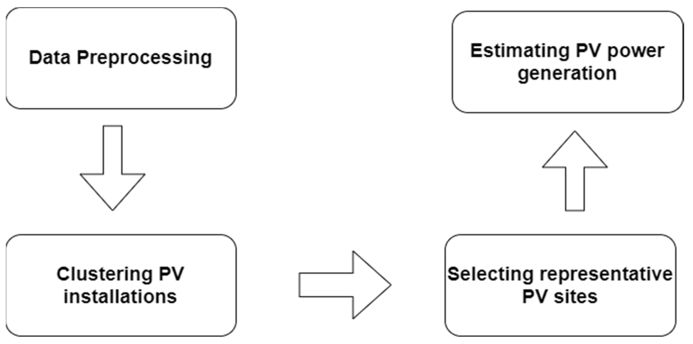
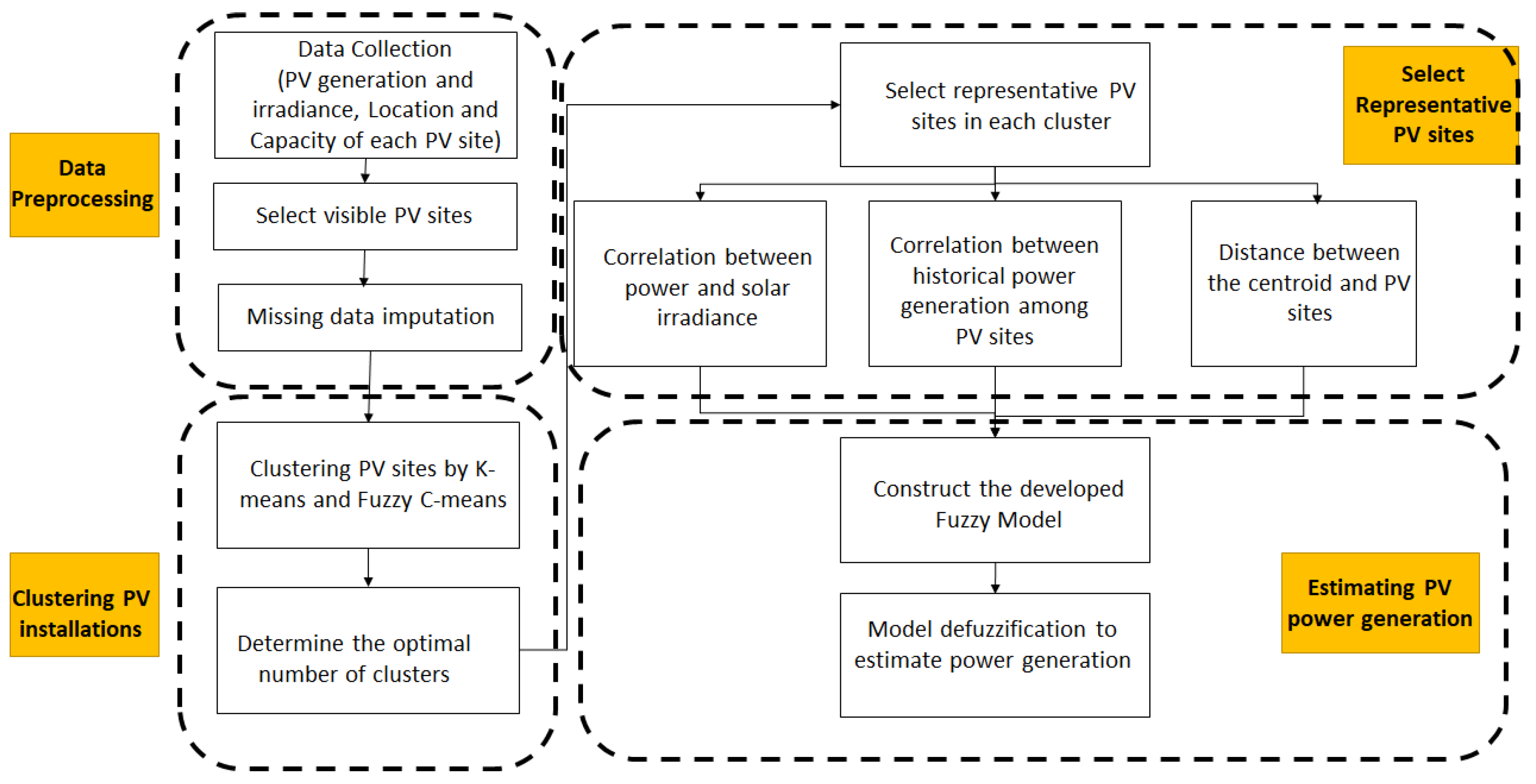
In this study, a fuzzy model-based approach is modified to estimate the invisible PV power generation in Taiwan. The proposed methodology consists of four major steps as demonstrated in Figure 1, i.e., data preprocessing, clustering, selecting of representative PV sites, and estimating invisible PV power production. The detailed information for each process, which comes with descriptive information, can be seen in Figure 2. In the stage of data preprocessing, after collecting the related data from all the accessible PV sites, several PV sites were identified as visible PV installations, and the K-Nearest Neighbor (KNN) approach was used to preprocess the missing and outlier measurement data in the raw dataset. Then, the second stage, i.e., clustering the PV installations, was implemented using different clustering algorithms; solar PV sites in Taiwan are then grouped into different clusters based on geographical conditions; moreover, the optimal number of clusters were also determined during this step. Following that, multiple representative PV sites in each cluster were determined based on a range of significant characteristics, including solar irradiance, historical power generation, or geographical coordination. Finally, historical power generation from these representative sites was used to construct the proposed fuzzy model, which estimates a total PV power generation in a cluster or region.
2.1. Data Preprocessing Using KNN Algorithm
It is notable that renewable energy measurement data are frequently missing owing to a variety of reasons, including the failure of measurement equipment, lack of internet connectivity, and PV modules that are out of operation or unavailable. Particularly, when measurement data are collected from a large number of PV installations, missing data are unavoidable. Hence, many approaches, such as KNN, for dealing with missing data of power generation have been discussed and compared in [20]. The KNN algorithm is a machine learning-based method, which calculates the distance-weighted average of the kth nearest data points according to the Euclidean distance to fill in the missing data [7]. The calculation equations are expressed as follows (1–3) [21]:
where is the filled value of missing data; is the number of neighboring data (); is the kth nearest observation to the missing value based on the Euclidean distance calculation; is the weight of the kth nearest , which is inversely proportional to the square of the distance to the neighboring data, as shown in Equation (2); is the Euclidean distance, which is defined as follows:
2.2. Clustering Techniques for PV Sites
After preprocessing the raw dataset, the PV installations in a given region were divided into sub-regions based on their geographical locations. It was expected that the PV locations at the same sub-region or cluster would have similar weather conditions, and hence their power generation would be highly correlated. In this study, K-Means and fuzzy C-Means clustering techniques were employed to obtain the sub-regions. However, for both techniques, depending on the number of clusters, a significant impact on the clustering effect could be observed. Generally, in most practical problems, the number of clusters is unknown. As a result, the Calinski–Harabasz index was used in this paper to identify the appropriate number of clusters before the clustering process.
2.2.1. Determine the Optimal Number of Clusters
The Calinski–Harabasz (CH) index is determined using the degree of dispersion between clusters, the distance between cluster points, and its cluster centroid [22,23,24]. The CH index is calculated as follows:
where s is the number of clusters; N is the number of PV sites; is the measure of dispersion between clusters; is the measure of dispersion of data within a cluster. and are defined as follows:
where is the number of PV sites in cluster s, is the center of cluster s, is the center of all PV sites, and the PV site i in cluster s. As various numbers of clusters, s, are substituted into Equation (5), the optimal number of clusters s, is obtained when the CH value is the smallest.
2.2.2. K-Means Clustering
The K-Means clustering technique is an unsupervised learning approach that is commonly used to partition a set of data X into several subsets. Furthermore, K-Means is a hard clustering technique, which indicates that each data point is assigned to a single set. This technique determines the clustering effect by minimizing the objective function that is given by:
where k is the number of clusters; is the number of all dispersed points in the ith cluster; x is any of the points in the ith cluster, and is the centroid of the ith cluster.
In this study, the actual location information, including latitude and longitude, of all PV installations was used as input data of the K-Means clustering technique.
2.2.3. Fuzzy C-Means Clustering
The fuzzy C-Means (FCM) clustering approach incorporates fuzzy logic into the K-Means clustering technique, which is frequently employed in PV or power system applications [25,26,27]. This is a soft clustering algorithm that achieves fuzzification by combining the membership value with the fuzzy m-value. It makes data clustering more flexible, allowing data belonging to several clusters at the same time, with different degrees of membership. The objective function of FCM is shown as follows [28]:
where represents the membership degree of the pattern belonging to the cluster; is the data point of dataset X; n is the number of dataset X; s is the number of clusters, and is the cluster centroid. Additionally, the fuzzy m-value (m ≥ 1) can regulate the impact of on the cluster centroid computation and repeatedly compute the value, to reach the optimal objective function.
2.3. Selection of Representative PV Sites within a Cluster
It is difficult to obtain the power generation from all the PV sites in a region or an area, therefore, by selecting a subset of PV sites with power outputs that could be considered as the representative of regional PV solar production is critical. These representative installations require consistent data as a reference for estimating the power generation in the whole region.
There are three essential factors for selecting representative PV sites that are commonly employed in the literature. They include historical power generation, location, and average solar irradiance. The Pearson Correlation Coefficient (PCC) is a popular method for calculating the correlation between two data sets [29]. In this study, the correlation coefficient , between the historical power generation of a single PV plant and the total historical power generation of all PV plants in the cluster, was derived as the following equation:
where is the historical power generation of a single PV plant n in cluster s, is the total historical power generation of all visible PV plants in the cluster; is the covariance between and ; and are the standard deviation of and , respectively.
Moreover, the relationship between the historical power generation and solar irradiance is also analyzed, which can be expressed as:
where is the average irradiance of cluster s.
In this study, three representative PV plants in each cluster with the highest values were selected, and then their real-time power generation outputs were fed into a fuzzy model to further estimate the aggregated or total PV power generation of the respective cluster or a whole region.
2.4. Modified Fuzzy Model for Power Generation Estimation
The significant advantage of our proposed modified fuzzy model is that it can estimate the total power generation using limited information from a small number of visible PV sites while maintaining an acceptable low level of estimation error. In this study, this model served as the foundation for predicting the PV power generation for all the PV sites that include visible and invisible generation.
It is true that PV installations that are located close to each other usually have similar weather conditions [30]. The proposed model used this concept to establish a probability distribution of the generation relationship between PV plants to establish the membership function, instead of using the “if-then rule” in a traditional fuzzy-logic algorithm. According to the historical power generation data from visible PV plants, the power generation relationship between any two PV plants can be obtained by using the following equation:
where αmn (t) is the relationship between power generation at time t for any two PV plants m and n in the cluster, and are the amount of power generation that is measured in the PV plant m and PV plant n at time t, respectively. and are the installed capacity of plant m and plant n, respectively.
The time period that was considered in this study was from 8 a.m. to 4 p.m., with data collected at 5-min intervals, which is the period that covers the majority of the daylight period and has a significant amount of solar power generation. The above-mentioned historical power generation can be used to obtain the distribution of the power generation relationship between plants m and n over a period of time. However, several factors affect the distribution curve of , including the distances between PV plants, and the installed capacity of power generation at each PV plant. For instance, the distribution of will be more concentrated when two PV plants are selected in close proximity to each other. Besides, the distribution of will be more extensive due to the similarity of solar irradiation.
After obtaining the probability distribution of , the next step is to establish the fuzzy numbers. A fuzzy set is described as a set in which the entirety of its members possesses a membership degree, most commonly with an interval of (0, 1). Moreover, a membership function is composed of the membership degrees of all the members in a fuzzy number, which is characterized by containing only one incremental segment and one decremental segment [31]. In practical applications, if the probability distribution curve is normalized with a curve that satisfies the characteristics of a fuzzy number and the membership interval is (0, 1), then it is regarded as a fuzzy number . The moving average smoothing method is commonly employed in probability distribution curves to improve the curves and fit the characteristics of fuzzy numbers.
Based on the definition of fuzzy numbers, this study used the probability distribution of to establish the fuzzy number , which can be differentiated according to ten different power generation levels (from 0 to the maximum value of 1, which is the per-unit (pu) value). The procedures for establishing the fuzzy number are listed as follows:
- In all the clusters with s = {1, ..., S}, is calculated for any two combinations of known PV plants m and n, as shown in Equation (14);
- The value of pn(t)/cn is calculated to determine which power generation level the PV plant n belongs to at time t for , in which there are ten levels, from 0 to the maximum value of 1 (pu value) in an ascending order. If the calculated pn(t)/cn values fall within the same range of values (e.g., 0.1 (level 1) or 0.3 (level 3)), then the values are classified in the same distribution;
- The values of the different generation levels are included into the distribution of that level. As a result, there will be a total of ten distributions in a cluster s;
- The ten probability distribution curves, , are normalized to (0, 1) and are redrawn;
- The normalized ten probability distributions are further processed through the moving average smoothing method to fit the characteristics of fuzzy numbers.
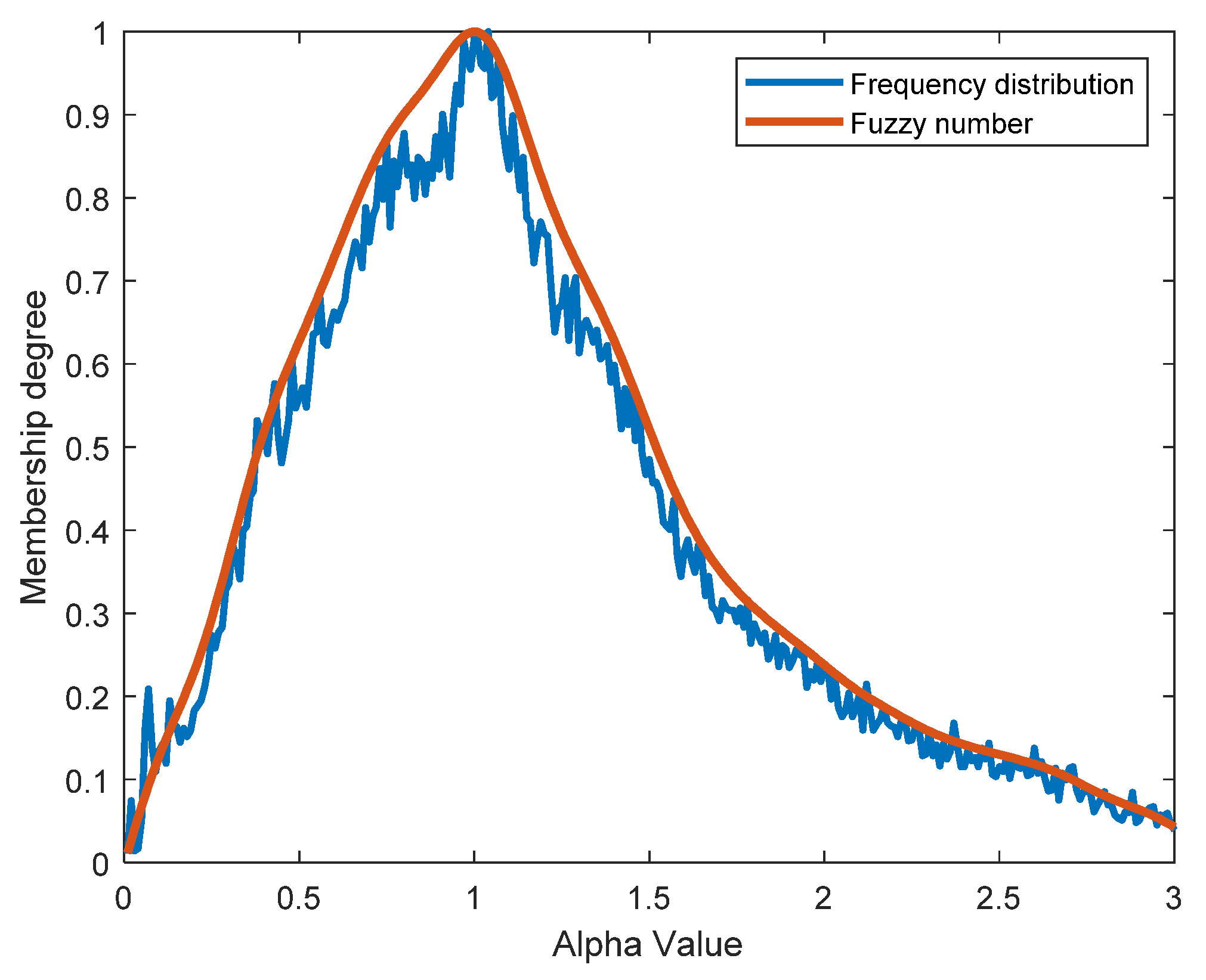
Following the above steps, all the fuzzy numbers can be calculated for different clusters s and different power generation levels g. As demonstrated in Figure 3, represents the probability distribution of the fuzzy number for the 3rd cluster between 0.2 pu and 0.3 pu of power generation. However, the probability distribution in is not smooth, so the moving average smoothing is used, as shown in the red curve in Figure 3.
After establishing the fuzzy number, , for each cluster, the fuzzy model is utilized to estimate the power generation by inputting the real-time power generation of the representative PV plants, along with the installed capacity of all visible and invisible PV plants in the cluster. Particularly, the fuzzy power generation, , of the cluster s is obtained by the following equation:
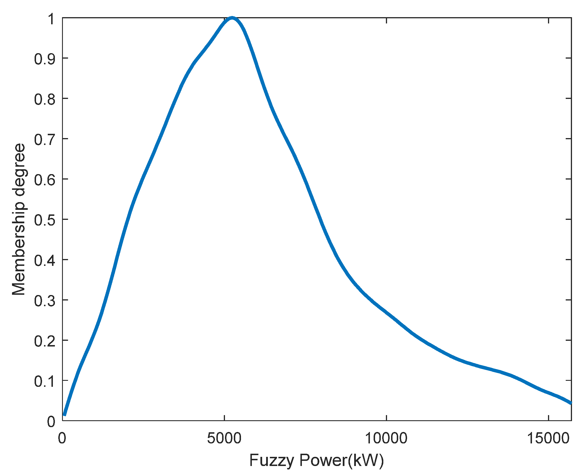
where is the fuzzy number corresponding to the power generation level g of the representative PV plants in cluster s; is the total installed capacity of all the visible and invisible PV plants in cluster s; is the sum of the power generation of the three representative PV plants in cluster s at time t; and is the sum of the installed capacity of the three representative PV plants in cluster s. Figure 4 shows the distribution of fuzzy power generation that is obtained from the 3rd cluster at power generation level 3.
After obtaining the total fuzzy power generation distribution for all PV plants in each cluster, the power generation estimation is obtained by de-fuzzification. The de-fuzzification is the procedure of converting the fuzzy distribution into a specific value. In the literature [10], the center of gravity method was used for de-fuzzification, which divides the area of the membership function into several sub-regions and then calculates the center gravity of the membership function. The center of gravity is defined as follows:
where indicates the sample element and is the aggregated output membership function. In this study, the center of gravity method that is proposed in the literature [10] was replaced by using the area equalization method for de-fuzzification. The area under the membership function curve was divided into two regions with the same size of area. The definition of in (16) that is obtained by de-fuzzifying the value with the area equalization method is expressed as:
Finally, the total power generation of all the PV plants in a whole region was obtained by summing all estimated power generation in each cluster.
3. Results and Discussion
3.1. Data Description and Model Construction
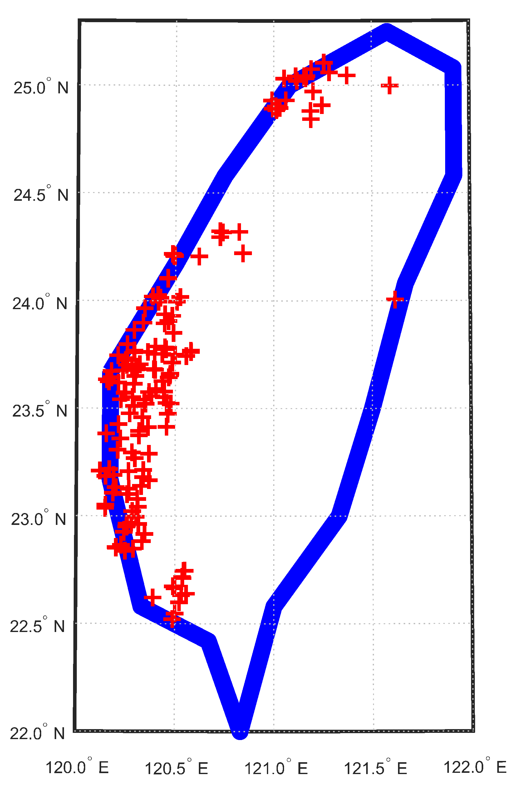
This study estimates the power generation with reference to the data of 169 PV plants in Taiwan, from November 2018 to April 2019. The geographical location of each PV plant is illustrated in Figure 5; this figure includes the map of Taiwan which reveals the distribution of all the PV sites with latitude and longitude coordinates; each cross symbol indicates a PV site. It is hard to show the detailed location of each PV site from Figure 5, but it can be observed that most PV sites are located at central and southern Taiwan.
The daily measurement data concerning the power generation and irradiance were recorded from 8:00 a.m. to 4:00 p.m. with a 5-min interval. The capacity of each PV plant ranged from 40 kW to 13 MW. The missing or outlier data within this period were processed by KNN algorithm.
In this work, it was assumed that 50% of the 169 PV sites were randomly selected as visible PV sites; in these visible PV sites, the historical power generation and irradiance measurements were used to select the representative PV plants and establish our fuzzy model. In contrast, the remaining 50% of PV sites that were assumed to be partially accessible, for their generation capacities and geographical locations, were designated as invisible PV sites.
The detail about the geographical location of each PV site is confidential, thus, this paper cannot show the respective information.
Regarding the selection of the representative PV plants, this study selected various numbers of representative plants for power generation estimation. The results indicated that as the number of representative plants in each cluster increases, a more accurate overall power generation estimation is obtained. In practice, however, the percentage of PV plants with real-time power generation measurements was very limited, thus, in this study, only three representative PV sites were determined to estimate the power generation using the fuzzy model. This will demonstrate that, despite the usage of a small amount of data from PV sites, artificial intelligence-based approaches could still be utilized to obtain an acceptable power generation estimation to tackle the problems of insufficient measurement data. For evaluating the estimation error, the daily mean absolute error (DMAE) was used as the power generation evaluation.
The model for PV power estimation was trained and constructed using measurement data from visible PV installations for one month, and then the power generation was estimated for the next month. Data from each previous month were utilized for training since the weather conditions are more similar during two consecutive months, and thus the power generation pattern is comparable. In the following section, various methods, including clustering, selecting representative PV plants, and de-fuzzification, are compared to improve the accuracy of power generation estimation. According to the analysis results, the number of clusters is restricted to four; thus, if the number of clusters are reduced, the number of PV plants in each cluster is increased. Since three representative PV plants are selected for each cluster, the total number of representative PV plants was 12 in this study.
The number of clusters was limited to four, since the authors assumed a lower bound of four clusters when conducting the study. In theoretical issues, the lower bound for cluster number is two. However, in this work, the PV sites are dispersed from north to south Taiwan, and the distance is approximately 400 km. Therefore, two clusters are too small to analyze the proposed problem since each cluster covers around 150–250km long. By contrast, owing to the limited PV sites in this study, if the cluster number is large, the PV sites are less within each cluster, which makes it difficult to experience a more obvious distinction when selecting different representative sites in each cluster. Therefore, the lower bound of cluster number in this work was set to four, and a total of 12 representative sites were selected.
3.2. Comparison of K-Means and Fuzzy C-Means Clustering Methods
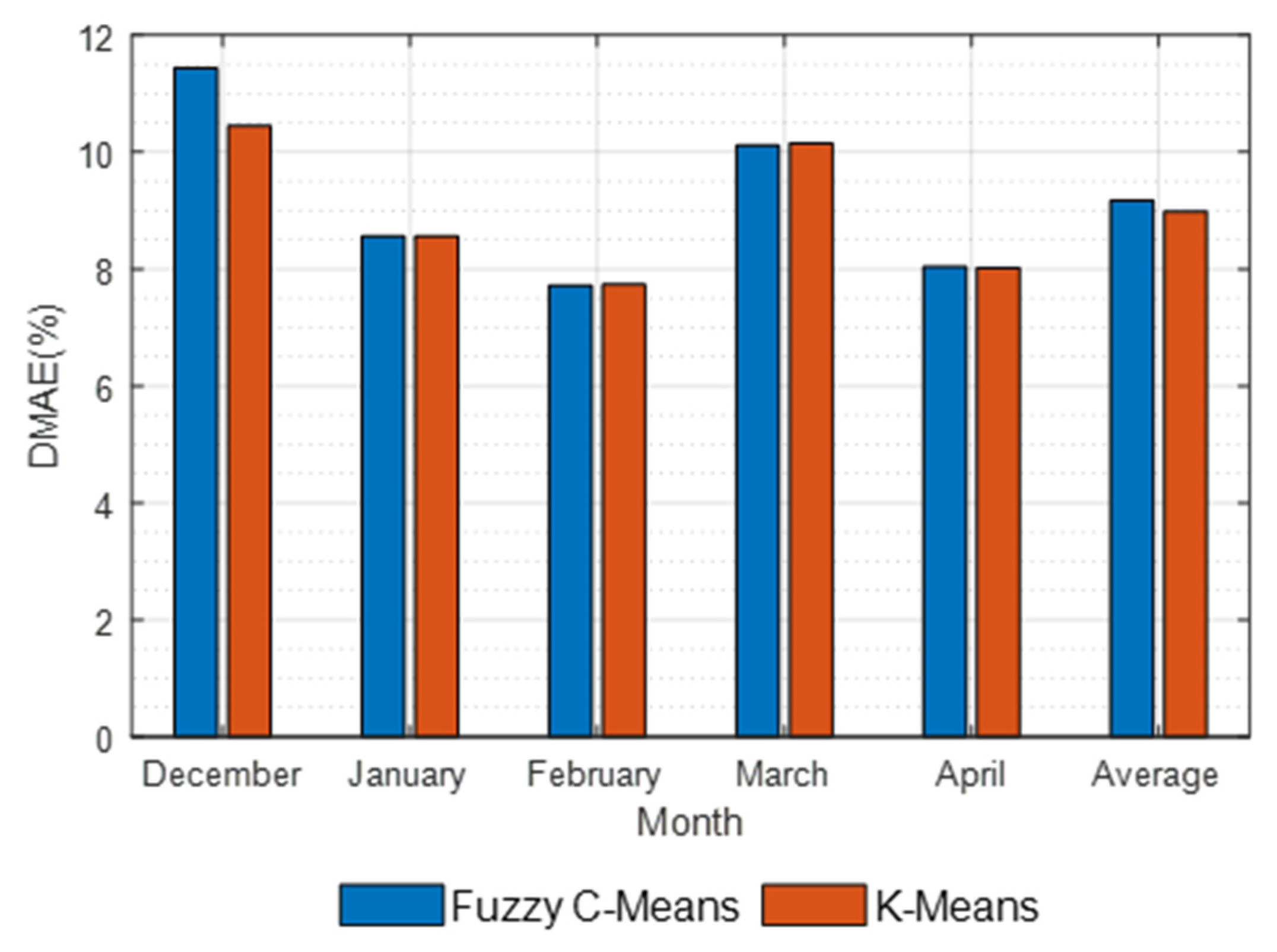
For cluster classification, the results by K-Means and fuzzy C-Means methods were compared. Table 1 demonstrates the number of PV sites in each cluster as determined by the two different clustering methods, which included K-Means and fuzzy C-Means; for instance, the number of PV sites in cluster 1 was 27 and 23 by K-Means and fuzzy C-Means, respectively. The results demonstrate that there was no substantial difference between the two clustering algorithms in determining the number of PV sites in each cluster. This indicates that the estimation results that were achieved by both clustering methods are comparable, as shown in Figure 6.
Figure 6 demonstrates the estimation error under the different cluster methods. After estimating the total power generation of all the PV plants in each cluster and summing them, the total estimation error was calculated based on the actual total power generation. In practical applications, it is impossible to know the actual total power generation from all the PV sites and obtain error statistics. The error calculation here was only to investigate the performance of the proposed methods.
The results revealed that the difference between the estimates that were obtained using the two clustering methods were not significant, indicating that the employment of any of the clustering algorithms is not a key factor of influence when dealing with a small number of clusters. Furthermore, Figure 6 demonstrates that the estimation errors were high in December and March, reaching more than 10%, while the estimation error was the lowest in February, which was about 7.5%. These differences in errors among the different months may be related to the fluctuation of weather variability.
3.3. Various Methods of Selecting a Representative PV Plant
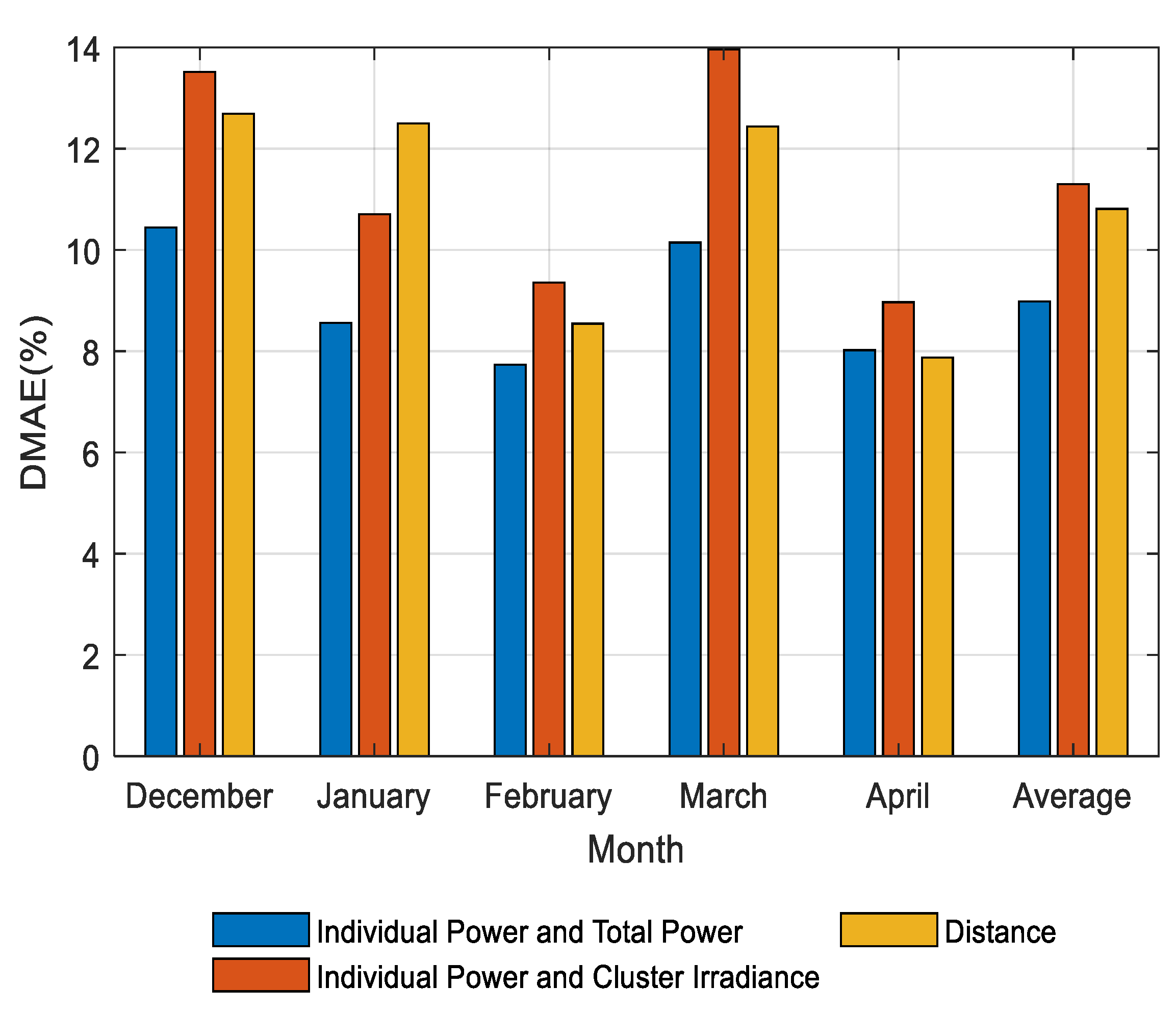
Numerous factors for PV power estimation were taken into consideration in this study. These factors included the correlation between the power generation of a single plant and the total power generation; the relationship between the power generation and solar irradiance; and the distance among the PV sites. Figure 7 shows that the lowest estimation error by selecting the representative PV plants was obtained according to the correlation between power generation. This demonstrates that historical power generation is the most essential variable when choosing the representative PV sites.
3.4. Comparison of Different De-fuzzification Methods
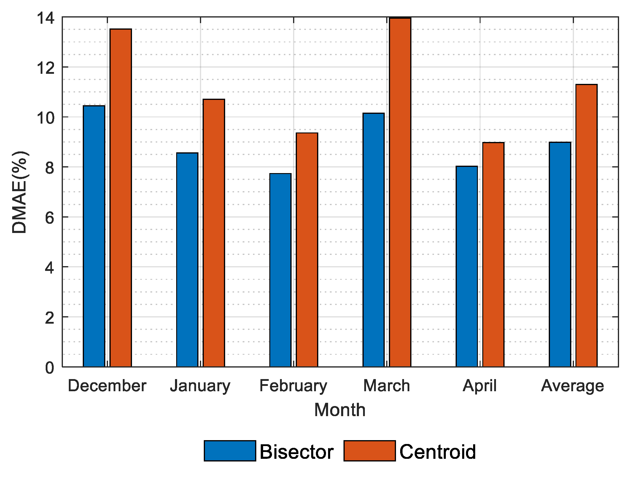
In this study, the center of gravity (centroid) method and the area equalization (bisector) method were used for de-fuzzification. Figure 8 shows that the area equalization method can achieve higher accuracy than the center of gravity method, so the area equalization method was selected for de-fuzzification of PV estimation in this study.
3.5. Advantages of using Fuzzy Models for Power Generation Estimation
This section shows the results with or without the proposed fuzzy model, to demonstrate the effectiveness of the fuzzy model in improving the estimation of invisible PV power generation. If the proposed fuzzy model was not implemented, the total power generation estimation for all PV plants is defined as follows:
where is the sum of the power generation from three representative PV plants at time t, is the total installed capacity of the three representative PV plants, and is the installed capacity of all PV plants for each cluster s.
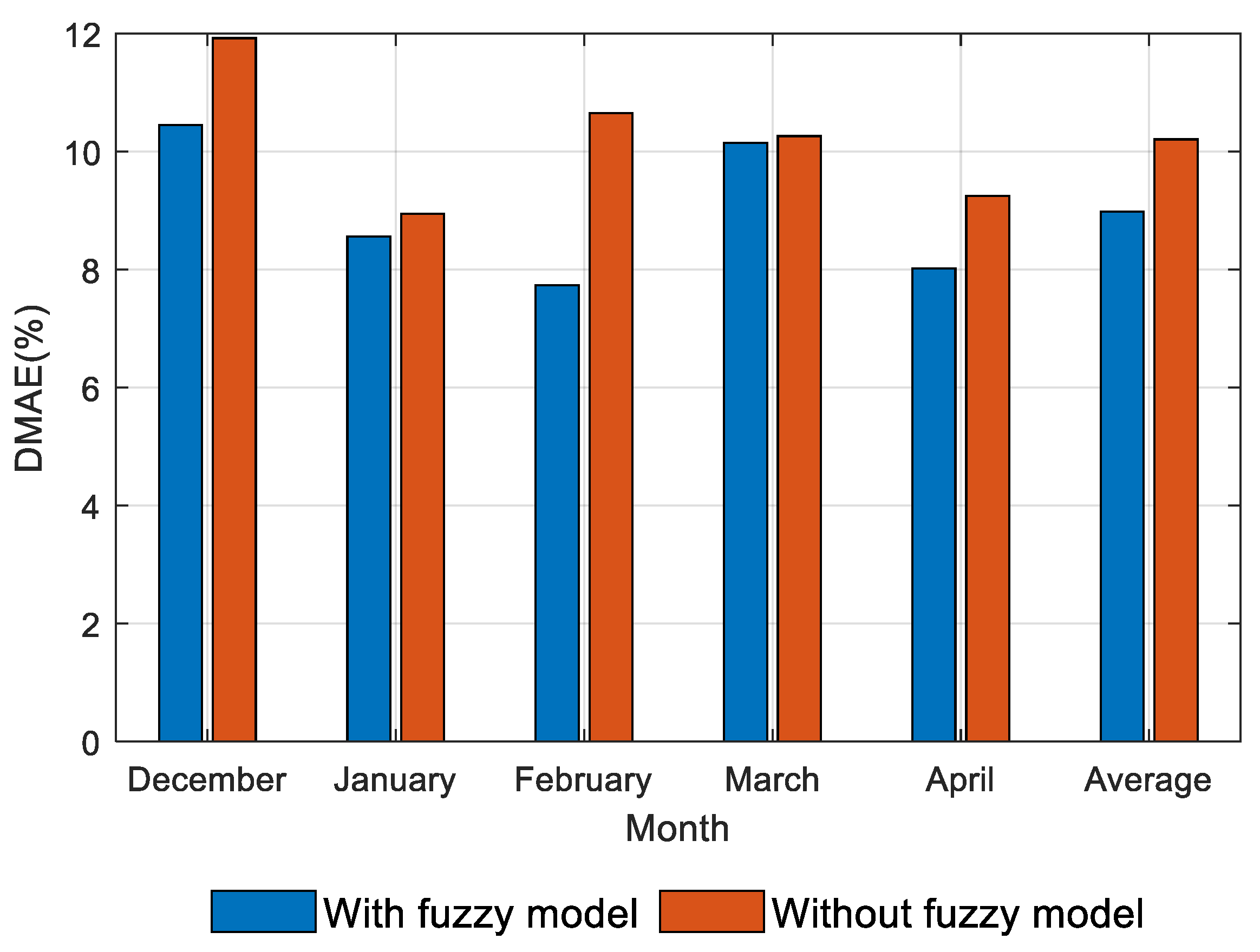
The above equation mainly uses the actual power generation of a representative PV plant and scales it equally to the total power generation that is estimated from the cluster by considering the ratio of its installed capacity. Figure 9 illustrates that the error of power estimation is reduced in all the months by using the proposed fuzzy model, especially in February, where the error is reduced by 2.92%, which highlights the effectiveness of the proposed fuzzy model in this application.
3.6. Results of Optimized Power Generation Estimation
According to the above results, the following model settings were implemented to optimize the estimation of PV power generation:
- The K-Means clustering method was used to cluster the PV plants;
- The area equalization method was used for de-fuzzification;
- The representative PV plants were selected with the highest correlation between the power generation of a single PV plant and the power generation of PV plants that have real-time measurements in the cluster;
- The number of representative PV plants in each cluster was three;
- The Calinski–Harabasz (CH) index was used as an index to determine the number of clusters.
Although four clusters were utilized in this study, more clusters could be better for PV power estimation in practice, i.e., the closer the plants in the same cluster, the more similar the power generation characteristics. Therefore, this study obtains the optimal number of clusters using the CH index. According to the calculation, the number of clusters was 19. With this number of clusters, in most cases, the maximum distance between any two PV sites in a single cluster does not exceed 20 km. Table 2 shows that by increasing the number of clusters in some months, such as December and April, it can significantly reduce the error of PV power estimation. However, increasing the number of clusters may have certain practical restrictions, such as the requirement to increase the overall number of representative PV plants, as well as the necessity for more reliable measurement data. If 19 clusters are determined, the number of representative PV plants increases significantly to exceed 50, which requires a significant increment in hardware construction and complexity of measurements. Nevertheless, the power estimation by 19 clusters only improves the error about 1.91% compared to the estimation by 4 clusters (only requires 12 representative PV plants in total). Furthermore, if the number of clusters increases, the number of PV plants at each cluster will be smaller. This indicates that there will be fewer PV plants to construct the fuzzy relationship at each cluster, which may reduce the accuracy of solar power estimation. In short, utilizing fewer clusters and representative PV plants would increase the estimation error, but it would be more efficient and useful in practice.
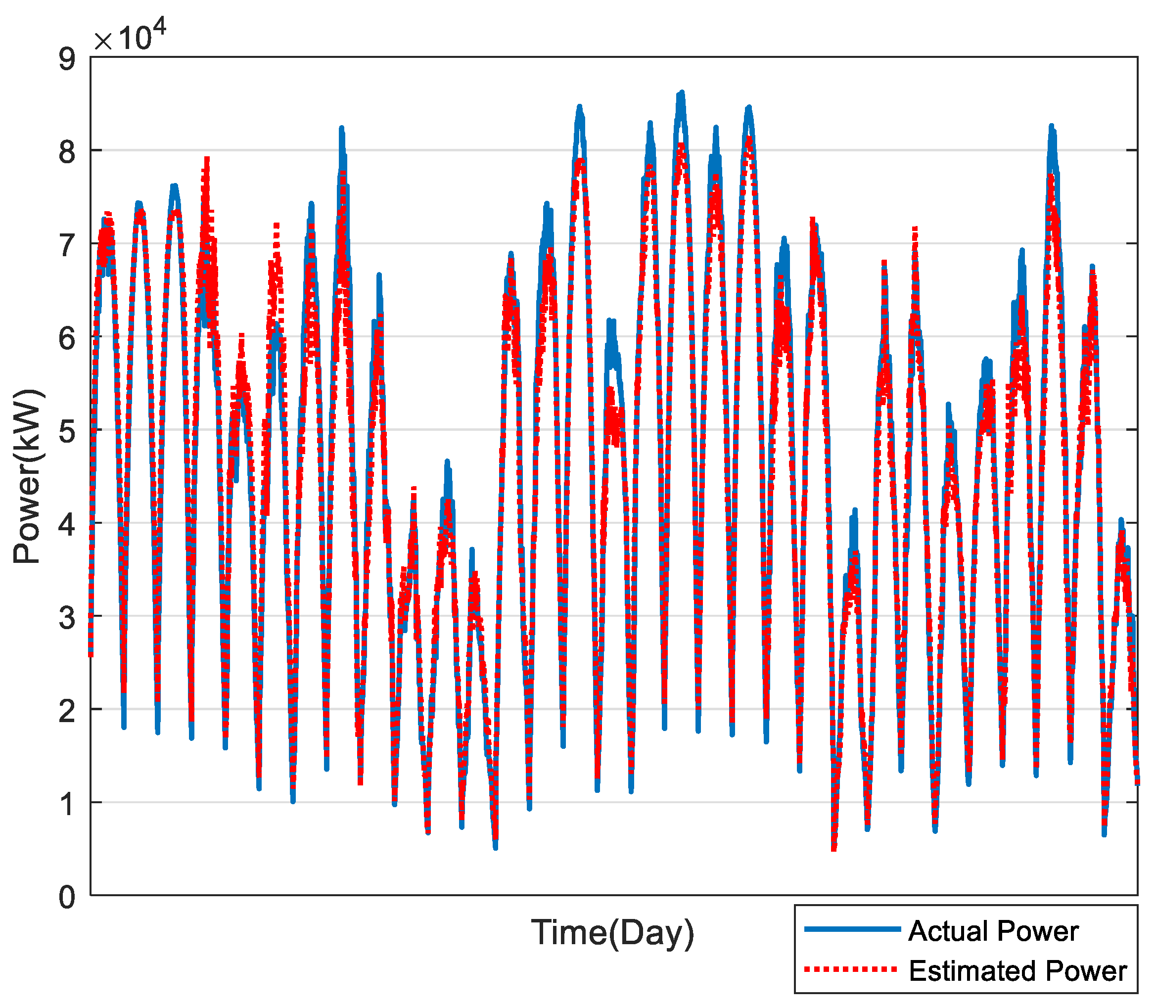
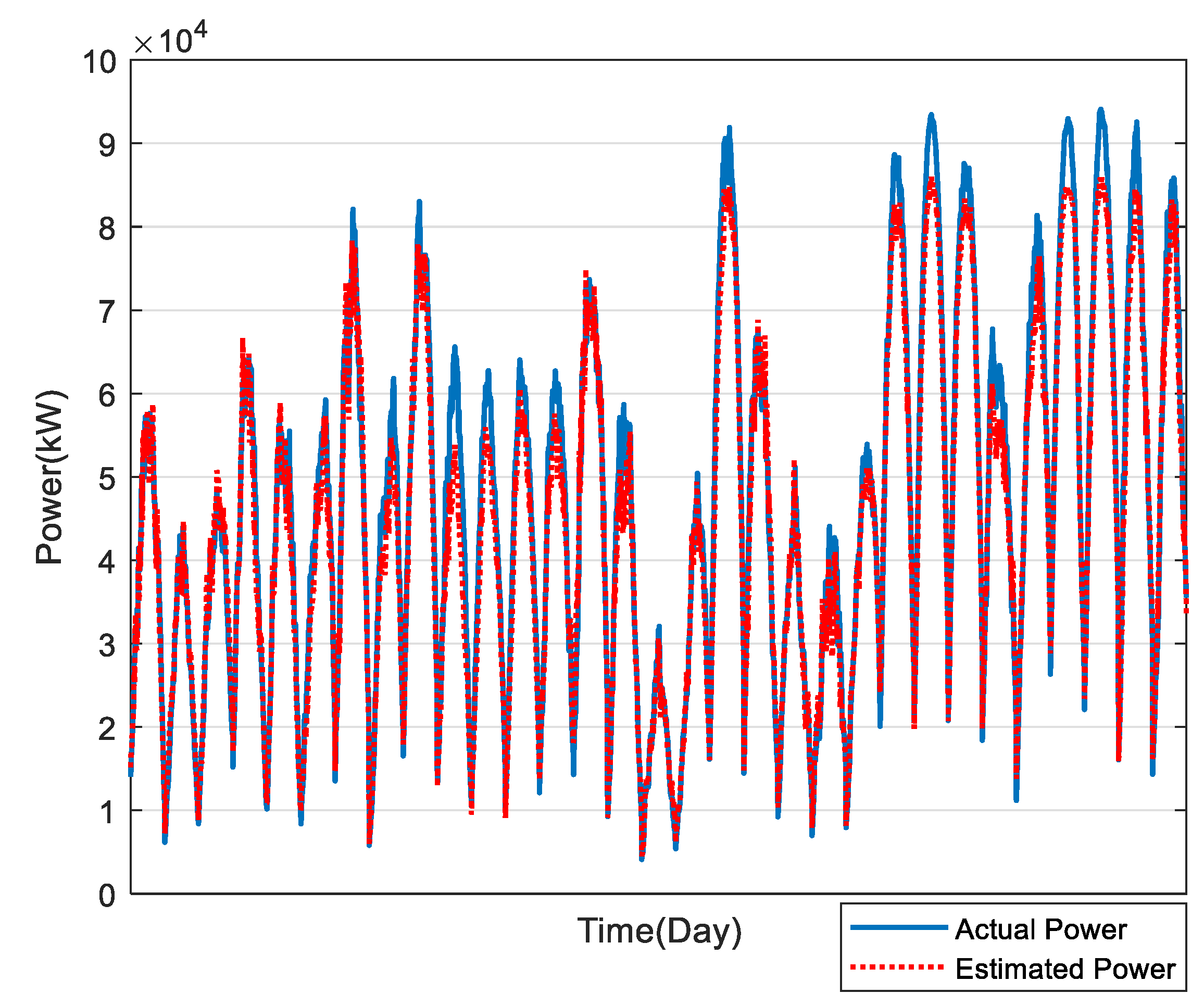
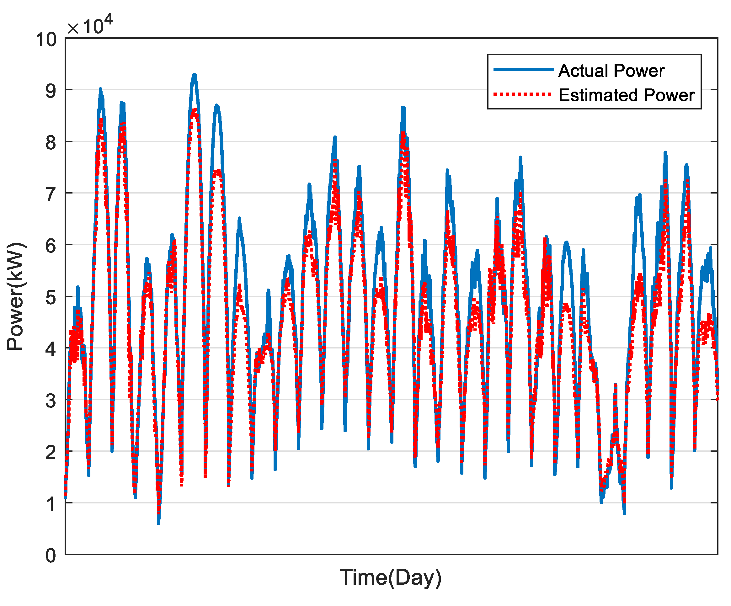
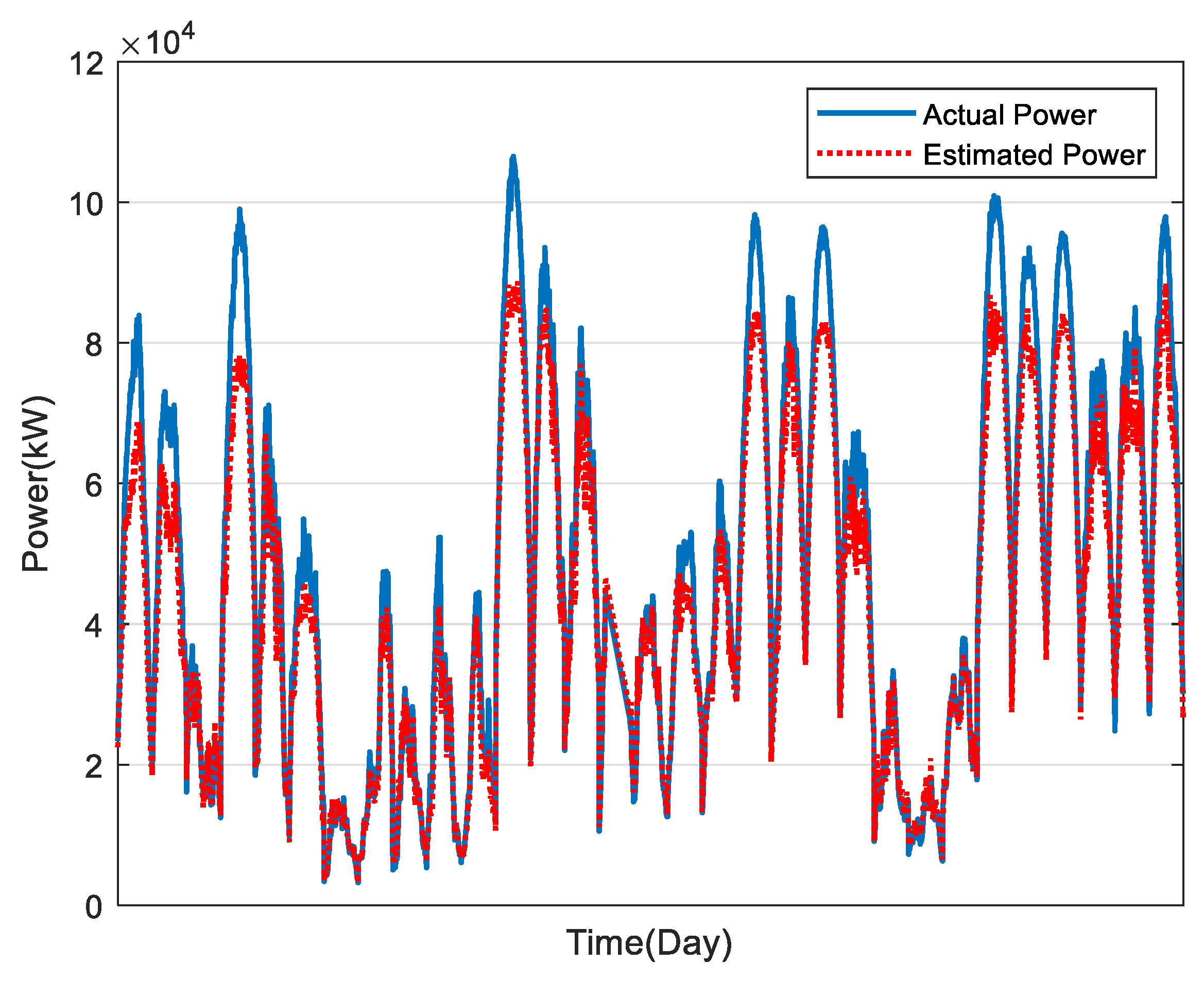
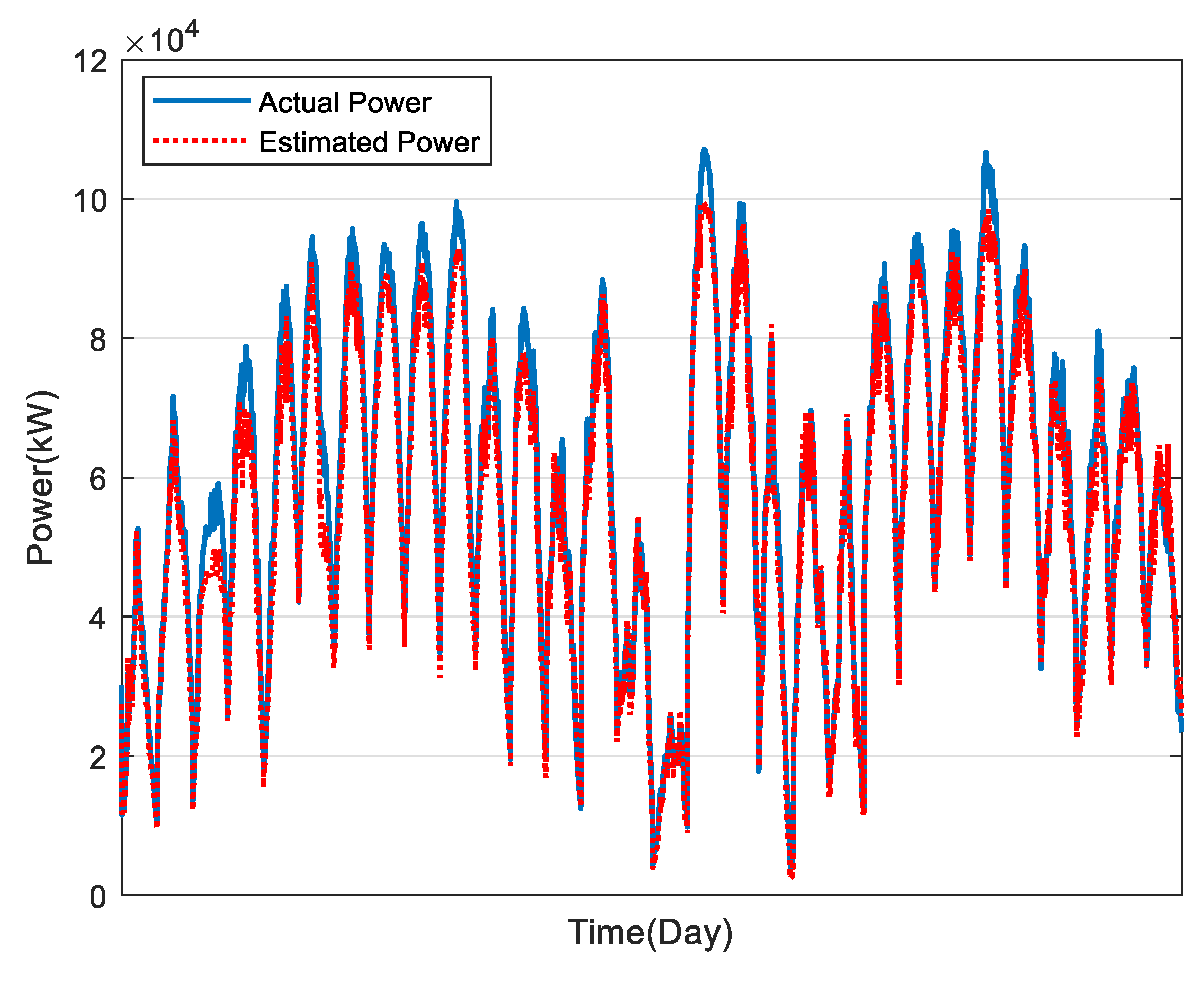
In this study, the estimation of power generation of 169 PV plants in Taiwan was calculated, as shown in Figure 10, Figure 11, Figure 12, Figure 13 and Figure 14, for December to April, respectively. The average estimation error of total PV power generation for the five months was 7.07%.
Different number of clusters will lead to different representative sites in total; consequently, the estimation results are also affected. Based on the analysis of the results, the power estimation by 19 clusters can be improved by only 1.91% compared to the estimation by four clusters. Although the former experiences an increase in accuracy, the improvement is not remarkable. That is, if more clusters are considered, fewer PV sites will appear in each cluster, which makes it difficult to build the relationship among the PV sites. Therefore, a lower bound of the clusters may provide a lower accuracy for PV generation estimation but it would be more efficient and practical.
More clusters across the area of 169 PV sites could obtain an accuracy estimation. However, if the number of clusters exceeds 20, too few PV sites appear in certain clusters. Thus, only the number of clusters from 4 to 20 has been tested in this work. The results demonstrate that the optimal number of clusters is 19, in which the maximum distance between two PV sites in the same cluster does not exceed 20 km. Notably, the PV sites in the same cluster should be close to each other since the atmospheric conditions in the same cluster should be similar. Therefore, it is reasonable for 19 clusters. However, as mentioned earlier, the power estimation by 19 clusters can be improved by only 1.91% compared to the estimation by four clusters. As for the lower limit about the number of clusters, this work suggested the appropriate number of clusters is four because it cannot obtain the optimal PV estimation if the lower number of clusters is in the range from two and five. In other words, the optimal number of clusters to achieve the highest accuracy is 19, but four clusters can achieve a more efficient and practical PV estimation.
In this section, this study has provided a complete comparison to demonstrate the technical contributions of the proposed method. These comparisons include different clustering methods, different methods to select representative PV sites, and the comparison between the proposed modified fuzzy model and traditional fuzzy model. Based on the above comparisons, this work proposed an optimized power generation estimation framework for invisible PV sites.
3.7. Discussions
According to the results of this study, the following observations are worth further discussion:
- The important steps for estimating invisible PV power generation include the selection of cluster number, the identification of representative PV plants in each cluster, and the estimate algorithm to be utilized. In this paper, a modified fuzzy model is proposed for the estimation of invisible PV power generation;
- Cluster classification using K-Means or fuzzy C-Means is not significant in terms of the results by both methods. However, increasing the number of clusters is expected to reduce the error of estimation. Moreover, the stability of the data measurement is also important;
- The significant factors for selecting representative PV plants include the correlation between generation, solar irradiance, or distance. The results of this study reveal that using the correlation between the power generation of a single plant and the total power generation of the known plants in the cluster to select a representative plant can provide a more accurate estimation.
- The center of gravity method for de-fuzzification was used in the literature [2]. This study used the area equalization method, and its result outperforms the center of gravity method.
- Theoretically, the higher number of clusters and representative PV plants that are selected, the more accurate the results that can be obtained. However, it is necessary to consider the limits of practical applications, which includes the actual number of PV plants that are available for stable measurements, the relationship among the different clusters, etc. If more clusters are selected, there is a risk of inaccurate estimation owing to an insufficient number of PV plants or missing of measurement data.
- In recent years, it has become more challenging for power system operators to estimate total power generation because of many behind-the-meter (or so-called invisible) PV installations. The proposed model does not necessitate the historical total power generation. It establishes the relationship of historical power generation among the visible PV sites in each cluster using a modified fuzzy model, and then estimates the total power generation from PV systems. This work takes inspiration from [6,10] but enhances the estimation process about selecting representative sites and the training model to improve the estimation accuracy.
4. Conclusions
In recent years, the penetration of invisible PV installations in the power systems poses numerous challenges for power monitoring and dispatching; thus, it is essential to estimate the invisible PV power generation in a large area. In this paper, a modified fuzzy model with a complete procedure has been proposed for estimating invisible PV power generation. The proposed model does not require aggregate output in the training stage and less data are required for constructing the model. The numerical results demonstrate that the proposed method provides an acceptable estimating result with an average DRME of 7.07% during five consecutive testing months and outperforms the traditional upscaling method throughout all the testing periods.
To improve the quality of historical measurement data prior to the execution of the estimation method, the missing and outlier data have been processed in this work. Additionally, this work evaluated the influences of various clustering algorithms as well as various de-fuzzification approaches on the estimating performance, which assists in determining what advantages they can bring to specific scenarios. This work also provided an efficient method to determine the most useful factors that affect the selection of representative PV sites. Based on the numerical results, the proposed method has proven to be a simple, efficient, and fast approach to estimate the aggregated power generation within a region.
Author Contributions
Conceptualization, Y.-K.W. and Y.-H.L.; methodology, Y.-H.L.; software, Y.-H.L.; validation, Y.-K.W., N.T.B.P. and W.-S.T.; formal analysis, Y.-H.L., C.-L.H. and N.T.B.P.; investigation, Y.-K.W. and Y.-H.L.; resources, Y.-K.W.; data curation, Y.-K.W.; writing—original draft preparation, C.-L.H. and Y.-H.L.; writing—review and editing, Y.-K.W., N.T.B.P. and W.-S.T.; visualization, C.-L.H.; supervision, Y.-K.W. and W.-S.T.; project administration, Y.-K.W.; funding acquisition, Y.-K.W. All authors have read and agreed to the published version of the manuscript.
Funding
This research was funded by the Ministry of Science and Technology (MOST) of Taiwan, grant number MOST 109-2622-E-194-005.
Institutional Review Board Statement
Not applicable.
Informed Consent Statement
Not applicable.
Conflicts of Interest
The authors declare no conflict of interest.
References
- Bu, F.; Dehghanpour, K.; Yuan, Y.; Wang, Z.; Zhang, Y. A Data-Driven Game-Theoretic Approach for Behind-the-Meter PV Generation Disaggregation. IEEE Trans. Power Syst. 2020, 35, 3133–3144. [Google Scholar] [CrossRef] [Green Version]
- Stein, J.S. The Photovoltaic Performance Modeling Collaborative (PVPMC). In Proceedings of the 2012 38th IEEE Photovoltaic Specialists Conference, Austin, TX, USA, 3–8 June 2012; pp. 3048–3052. [Google Scholar]
- Chen, D.; Irwin, D. SunDance: Black-Box Behind-the-Meter Solar Disaggregation. In Proceedings of the Eighth International Conference on Future Energy Systems, Hong Kong, China, 16–19 May 2017; pp. 45–55. [Google Scholar]
- Kabir, F.; Yu, N.; Yao, W.; Yang, R.; Zhang, Y. Estimation of Behind-the-Meter Solar Generation by Integrating Physical with Statistical Models. In Proceedings of the 2019 IEEE International Conference on Communications, Control, and Computing Technologies for Smart Grids (SmartGridComm), Beijing, China, 21–23 October 2019; pp. 1–6. [Google Scholar]
- Kabir, F.; Yu, N.; Yao, W.; Yang, R.; Zhang, Y. Joint Estimation of Behind-the-Meter Solar Generation in a Community. IEEE Trans. Sustain. Energy 2021, 12, 682–694. [Google Scholar] [CrossRef]
- Shaker, H.; Zareipour, H.; Wood, D. A Data-Driven Approach for Estimating the Power Generation of Invisible Solar Sites. IEEE Trans. Smart Grid 2016, 7, 2466–2476. [Google Scholar] [CrossRef]
- Pierro, M.; De Felice, M.; Maggioni, E.; Moser, D.; Perotto, A.; Spada, F.; Cornaro, C. Data-Driven Upscaling Methods for Regional Photovoltaic Power Estimation and Forecast Using Satellite and Numerical Weather Prediction Data. Sol. Energy 2017, 158, 1026–1038. [Google Scholar] [CrossRef]
- Bright, J.M.; Killinger, S.; Lingfors, D.; Engerer, N.A. Improved Satellite-Derived PV Power Nowcasting Using Real-Time Power Data from Reference PV Systems. Sol. Energy 2018, 168, 118–139. [Google Scholar] [CrossRef]
- Wang, F.; Li, K.; Wang, X.; Jiang, L.; Ren, J.; Mi, Z.; Shafie-Khah, M.; Catalão, J.P.S. A Distributed PV System Capacity Estimation Approach Based on Support Vector Machine with Customer Net Load Curve Features. Energies 2018, 11, 1750. [Google Scholar] [CrossRef] [Green Version]
- Shaker, H.; Zareipour, H.; Wood, D. Estimating Power Generation of Invisible Solar Sites Using Publicly Available Data. IEEE Trans. Smart Grid 2016, 7, 2456–2465. [Google Scholar] [CrossRef]
- Kara, E.C.; Roberts, C.M.; Tabone, M.; Alvarez, L.; Callaway, D.S.; Stewart, E.M. Disaggregating Solar Generation from Feeder-Level Measurements. Sustain. Energy Grids Netw. 2018, 13, 112–121. [Google Scholar] [CrossRef]
- Zhang, X.; Grijalva, S. A Data-Driven Approach for Detection and Estimation of Residential PV Installations. IEEE Trans. Smart Grid 2016, 7, 2477–2485. [Google Scholar] [CrossRef]
- Sossan, F.; Nespoli, L.; Medici, V.; Paolone, M. Unsupervised Disaggregation of Photovoltaic Production from Composite Power Flow Measurements of Heterogeneous Prosumers. IEEE Trans. Ind. Inform. 2018, 14, 3904–3913. [Google Scholar] [CrossRef] [Green Version]
- Stainsby, W.; Zimmerle, D.; Duggan, G.P. A Method to Estimate Residential PV Generation from Net-Metered Load Data and System Install Date. Appl. Energy 2020, 267, 114895. [Google Scholar] [CrossRef]
- Wang, Y.; Zhang, N.; Chen, Q.; Kirschen, D.S.; Li, P.; Xia, Q. Data-Driven Probabilistic Net Load Forecasting with High Penetration of Behind-the-Meter PV. IEEE Trans. Power Syst. 2018, 33, 3255–3264. [Google Scholar] [CrossRef]
- Li, K.; Wang, F.; Mi, Z.; Fotuhi-firuzabad, M.; Dui, N.; Wang, T. Capacity and Output Power Estimation Approach of Individual Behind-the-Meter Distributed Photovoltaic System for Demand Response Baseline Estimation. Appl. Energy 2019, 253, 113595. [Google Scholar] [CrossRef]
- Cheung, C.M.; Zhong, W.; Xiong, C.; Srivastava, A.; Kannan, R.; Prasanna, V.K. Behind-the-Meter Solar Generation Disaggregation Using Consumer Mixture Models. In Proceedings of the 2018 IEEE International Conference on Communications, Control, and Computing Technologies for Smart Grids (SmartGridComm), Aalborg, Denmark, 29–31 October 2018; pp. 1–6. [Google Scholar]
- Shaker, H.; Manfre, D.; Zareipour, H. Forecasting the Aggregated Output of a Large Fleet of Small Behind-the-Meter Solar Photovoltaic Sites. Renew. Energy 2020, 147, 1861–1869. [Google Scholar] [CrossRef]
- Sun, M.; Feng, C.; Zhang, J. Factoring Behind-the-Meter Solar into Load Forecasting: Case Studies under Extreme Weather. In Proceedings of the 2020 IEEE Power and Energy Society Innovative Smart Grid Technologies Conference, ISGT 2020, Washington, DC, USA, 17–20 February 2020; pp. 1–5. [Google Scholar] [CrossRef]
- Kim, T.; Ko, W.; Kim, J. Analysis and Impact Evaluation of Missing Data Imputation in Day-Ahead PV Generation Forecasting. Appl. Sci. 2019, 9, 204. [Google Scholar] [CrossRef] [Green Version]
- Murti, D.M.P.; Pujianto, U.; Wibawa, A.P.; Akbar, M.I. K-Nearest Neighbor (K-NN) Based Missing Data Imputation. In Proceedings of the 2019 5th International Conference on Science in Information Technology (ICSITech), Yogyakarta, Indonesia, 23–24 October 2019. [Google Scholar]
- Caliński, T.; Harabasz, J. A Dendrite Method for Cluster Analysis. Commun. Stat. 1974, 3, 1–27. [Google Scholar] [CrossRef]
- Wang, X.; Xu, Y. An Improved Index for Clustering Validation Based on Silhouette Index and Calinski-Harabasz Index. In IOP Conference Series: Materials Science and Engineering; IOP Publishing: Bristol, UK, 2019; Volume 569. [Google Scholar] [CrossRef] [Green Version]
- Arbelaitz, O.; Gurrutxaga, I.; Muguerza, J.; Pérez, J.M.; Perona, I. An Extensive Comparative Study of Cluster Validity Indices. Pattern Recognit. 2013, 46, 243–256. [Google Scholar] [CrossRef]
- Sujil, A.; Kumar, R.; Bansal, R.C. FCM Clustering-ANFIS-based PV and Wind Generation Forecasting Agent for Energy Management in a Smart Microgrid. J. Eng. 2019, 2019, 4852–4857. [Google Scholar] [CrossRef]
- Mingoti, S.A.; Lima, J.O. Comparing SOM Neural Network with Fuzzy C-Means, K-Means and Traditional Hierarchical Clustering Algorithms. Eur. J. Oper. Res. 2006, 174, 1742–1759. [Google Scholar] [CrossRef]
- Liu, S.; Dong, L.; Liao, X.; Cao, X.; Wang, X. Photovoltaic Array Fault Diagnosis Based on Gaussian Kernel Fuzzy C-Means Clustering Algorithm. Sensors 2019, 19, 1520. [Google Scholar] [CrossRef] [Green Version]
- Hung, M.-C.; Yang, D.-L. An Efficient Fuzzy C-Means Clustering Algorithm. In Proceedings of the 2001 IEEE International Conference on Data Mining, San Jose, CA, USA, 29 November–2 December 2001; pp. 225–232. [Google Scholar]
- Benesty, J.; Chen, J.; Huang, Y.; Cohen, I. Pearson Correlation Coefficient. In Noise Reduction in Speech Processing; Springer: Berlin/Heidelberg, Germany, 2009; pp. 1–4. ISBN 978-3-642-00296-0. [Google Scholar]
- Camargo, M.B.P.; Hubbard, K.G. Spatial and Temporal Variability of Daily Weather Variables in Sub-Humid and Semi-Arid Areas of the United States High Plains. Agric. For. Meteorol. 1999, 93, 141–148. [Google Scholar] [CrossRef]
- Hanss, M. Applied Fuzzy Arithmetic; Springer: Berlin/Heidelberg, Germany, 2005; ISBN 3540242015. [Google Scholar]
Figure 1.
The proposed methodology.

Figure 2.
Detailed information for each process.

Figure 3.
Example of frequency distribution and fuzzy numbers .

Figure 4.
The fuzzy power generation .

Figure 5.
Geographical locations of 169 PV plants.

Figure 6.
DMAE value of all the PV sites using the different clustering methods.

Figure 7.
The results of selecting the representative PV plants using different factors.

Figure 8.
Estimation error of power generation with the different de-fuzzification methods.

Figure 9.
Estimation results with and without fuzzy models.

Figure 10.
Results of PV power estimation in December.

Figure 11.
Results of PV power estimation in January.

Figure 12.
Results of PV power estimation in February.

Figure 13.
Results of PV power estimation in March.

Figure 14.
Results of PV power estimation in April.


Table 1.
Number of PV plants that were obtained using the different clustering methods.
| Clustering Algorithm | Cluster 1 | Cluster 2 | Cluster 3 | Cluster 4 |
|---|---|---|---|---|
| K-Means | 27 | 48 | 71 | 23 |
| FCM | 23 | 48 | 68 | 30 |
Table 2.
Number of PV plants obtained using different clustering methods.
| Month | 4 Clusters (%) | 19 Clusters (%) |
|---|---|---|
| December | 10.45 | 5.90 |
| January | 8.56 | 6.00 |
| February | 7.73 | 8.51 |
| March | 10.15 | 8.99 |
| April | 8.02 | 5.94 |
| Average | 8.98 | 7.07 |
Publisher’s Note: MDPI stays neutral with regard to jurisdictional claims in published maps and institutional affiliations. |
© 2022 by the authors. Licensee MDPI, Basel, Switzerland. This article is an open access article distributed under the terms and conditions of the Creative Commons Attribution (CC BY) license (https://creativecommons.org/licenses/by/4.0/).
Share and Cite
MDPI and ACS Style
Wu, Y.-K.; Lai, Y.-H.; Huang, C.-L.; Phuong, N.T.B.; Tan, W.-S. Artificial Intelligence Applications in Estimating Invisible Solar Power Generation. Energies 2022, 15, 1312. https://0-doi-org.brum.beds.ac.uk/10.3390/en15041312
AMA Style
Wu Y-K, Lai Y-H, Huang C-L, Phuong NTB, Tan W-S. Artificial Intelligence Applications in Estimating Invisible Solar Power Generation. Energies. 2022; 15(4):1312. https://0-doi-org.brum.beds.ac.uk/10.3390/en15041312
Chicago/Turabian StyleWu, Yuan-Kang, Yi-Hui Lai, Cheng-Liang Huang, Nguyen Thi Bich Phuong, and Wen-Shan Tan. 2022. "Artificial Intelligence Applications in Estimating Invisible Solar Power Generation" Energies 15, no. 4: 1312. https://0-doi-org.brum.beds.ac.uk/10.3390/en15041312
Note that from the first issue of 2016, this journal uses article numbers instead of page numbers. See further details here.