
Recovery Algorithm of Power Metering Data Based on Collaborative Fitting

1
Electric Power Research Institute, State Grid Shanghai Municipal Electric Power Company, Shanghai 200051, China
2
School of Electrical Engineering & Automation, Jiangsu Normal University, Xuzhou 221116, China
*
Author to whom correspondence should be addressed.
Energies 2022, 15(4), 1570; https://0-doi-org.brum.beds.ac.uk/10.3390/en15041570
Submission received: 22 January 2022
/
Revised: 10 February 2022
/
Accepted: 15 February 2022
/
Published: 21 February 2022
(This article belongs to the Special Issue Frontiers in Advanced Power Equipment and Research in Condition Diagnostic and Sensing)
Abstract
:Electric energy metering plays a crucial role in ensuring fair and equitable transactions between grid companies and power users. With the implementation of the State Grid Corporation’s energy Internet strategy, higher requirements have been put forward for power grid companies to reduce costs and increase efficiency and user service capabilities. Meanwhile, the accuracy and real-time requirements for electric energy measurements have also increased. Electricity information collection systems are mainly used to collect the user-side energy metering data for the power users. Attributed to communication errors, communication delays, equipment failures and other reasons, some of the collected data is missed or confused, which seriously affects the refined management and service quality of power grid companies. How to deal with such data has been one of the important issues in the fields of machine learning and data mining. This paper proposes a collaborative fitting algorithm to solve the problem of missing collected data based on latent semantics. Firstly, a tree structure of user history data is established, and then the user groups adjacent to the user with missing data are obtained from this. Finally, the missing data are recovered using the alternating least-squares matrix factorization algorithm. Through numerical verification, this method has high reliability and accuracy in recoverying the missing data.
1. Introduction
In order to achieve sustainable green development, the strategic policy of energy conservation and emission reduction [1] has become urgent for China. Electric power occupies a large proportion and plays an important role in China’s energy sector. Lean management of power grids will help implement the national strategy. With the improvement of people’s living standard and industrial development, grid users have higher requirements for the service quality. Thanks to the progress of new energy technology and network technology, the traditional power grid is developing comprehensively into an energy network [2,3]. Various kinds of energy are converging in the grid, which makes the electric energy measurement complicated. For example, smart grids and microgrids are precisely the penetration of decentralized generation and consumption and require measurement and monitoring equipment. Moreno Escobar et al. [4] presented a survey of key aspects, technologies, protocols and case studies of the current and future trend of Smart Grids. They proposed a taxonomy of a large number of technologies in Smart Grids and their applications in scenarios of Smart Networks, Neural Networks, Blockchain, Industrial Internet of Things or Software-Defined Networks. Since various architectures lack experimental validation, the specification of involved equipment regarding an industrial/proprietary or open-source nature and the concretization of communication protocols, González et al. [5] proposed an innovative multi-layered architecture to deploy heterogeneous automation and monitoring systems for microgrids. Moreover, Förderer et al. [6] presented an analysis of options for integrating automated (Building) Energy Management Systems (EMSs) into the smart meter architecture based on the technical guidelines for SMGWs by the German Federal Office for Information Security. In order to improve the accuracy and real-time performance of remote electric energy measurement, advanced communication technology and information collection technology are used to upgrade the traditional electric energy measurement.
The electricity consumption information collection system should be conducive to enhancing the reliability of the user’s electricity quality and meeting their various electricity needs. However, in actual operation, some errors and loss of measurement data collected remotely will seriously affect the implementation of lean management work, including the line loss analysis of the power grid company, power supply reliability evaluation and equipment failure online monitoring. All of these pose a threat to electricity billing, customer service and the reliability of data that is used for supporting the government to make decisions.
The factors that affect the quality of centralized procurement mainly include hardware failures of system equipment and soft failures, including electromagnetic interference, communication errors and communication delays. When there is an abnormal situation, such as errors or missing data, in the collection of data, the power supply company needs to send staff to the site to collect the data again. When the number of users reaches a certain scale, this is both unrealistic and unnecessary. Because most of these abnormal data are brought by temporary and occasional soft faults, manual collection is very uneconomical in order to obtain the true data of an abnormal data point. Therefore, how to recover abnormal data based on existing data is a problem that needs to be solved urgently, and its accomplishment will receive huge economic benefits.
At present, many researchers have developed various kinds of techniques to recover the missing data. Those methods can be divided into two categories: interpolation and fitting. Jones et al. [7] used Lagrange interpolation to recover the lost data in the system. This algorithm has lower complexity and a faster calculation speed. However, the errors increase and the anti-interference ability becomes weak when the system changes dynamically. Ding et al. [8] applied several interpolation methods such as radial basis function, moving least-squares and adaptive inverse distance to recover the missing values of small-scale time series data. It has been proved that moving least-squares is a relatively efficient and accurate recovery algorithm. Unfortunately, the accuracy of this algorithm is highly dependent on the number of reference samples. Deng et al. [9] integrated linear interpolation with matrix combination and replacement so that an improved random forest method is proposed to recover a large amount of electricity data missed. The result indicated that the new algorithm has a better effect on data recovery in a linear system.
Some scholars are devoted to recovering missing data by means of fitting. Pan and Li [10] proposed a missing data fitting algorithm based on the temporal and spatial correlation of sensor data. The linear regression model is used to describe the spatial correlation of sensor data among different sensor nodes. The missing data are estimated depending on the data information of multiple neighboring nodes so as to obtain stable and reliable fitting performance. As a powerful tool for data fitting, deep learning can theoretically avoid the linear constraints in data fitting. Chai et al. [11] established a model architecture of a U-NET convolution neural network and successfully transformed incomplete data into the corresponding complete data. In this model, randomly sampled data and the corresponding complete data served as input and output, respectively. James et al. [12] proposed a new graph-based deep learning method and designed a graph-convolution recursive adjunctive network to process available information and extract the correlation between graph and time data. The power grid state is recovered and predicted in advance by using grid topology and existing measurement data. However, the complexity of deep learning is high, and the algorithm speed is not dominant. In contrast, the low-rank matrix [13] algorithm greatly simplifies the computational complexity of the recovery algorithm. Konstantinopoulos et al. [14] combined this low-rank matrix method with adaptive filtering and proposed a fast online algorithm for fitting missing data. Wang et al. [15,16] solved the data sparsity problem in the collaborative recommendation algorithm using the alternating least-squares method. Yang et al. [17] proposed a dynamic data component analysis method based on singular value decomposition and a recovery iterative calculation method based on training, verification and classification of lost data to achieve high-precision data recovery of single-channel PMU measurement information.
Due to the complexity and diversity of actual application scenarios, existing data recovery algorithms are designed for different applications.
In traditional matrix factorization (MF) algorithms, most of them use the objective function based on least-squares and perform gradient optimization to find the best value.
Frenich et al. [18] combined the alternating least-squares (ALS) algorithm with the orthogonal projection approach and positive matrix factorization to resolve HPLC-DAD data into individual concentration profiles and spectra. Within each data subset, a reduced number of species present made the resolution easier. Kim and Park [19] introduced an active set-based fast algorithm for non-negativity constrained least-squares with multiple right-hand side vectors for non-negative matrix factorization. Its convergence properties were discussed, and a rigorous convergence criterion was described. Zhao and Zhang [20] modified the previous method by a successive alternate technique and proposed a two-step projection method for solving the constrained problem of low-rank matrix factorization with missing data. The proposed algorithm called SALS is easy to implement and converges very fast, even for a large matrix. Liu et al. [21] proposed a modified strategy for alternating non-negative least-squares, which can ensure the sequence generated has at least one limit point. This limit point is a stationary point of non-negative matrix factorization. Lee and Pang [22] developed a multichannel blind source separation algorithm. The new algorithm modified the multi-channel non-negative matrix factorization model with stacked matrix notation and developed an alternating least-squares method. Giampouras et al. [23] came up with a generic low-rank promoting regularization function and designed a regularizer resulting from MF to promote low-rankness on the optimization problem. Depending on the new LRMF formulation, the problems of denoising and matrix completion are redefined and solved via efficient alternating iteratively reweighted least-squares type algorithms. Chen et al. [24] presented an efficient and portable ALS solver (clMF) for recommender systems. The fine-grained tiling technique, the thread batching technique and three architecture-specific optimizations are applied to achieve high performance. Belachew and Buono [25] combined the concept of alternating least-squares with the multiplicative update rules of a divergence-based P-NMF method. The new and generalized hybrid algorithm with remarkable clustering performances can provide highly “orthogonal” and very sparse basis factors that help to extract distinctive and better-localized features of the original data. Zhu et al. [26] proposed a method by alternating least-squares based on matrix factorization to predict lncRNA-disease associations. Based on a new sparse matrix format, Chen et al. [27] presented an efficient implementation of the alternative least-squares (ALS) algorithm for parallel matrix factorization. The repeated data loads are avoided by organizing the sparse matrix into 2D tiles. The data reuses are improved, and a data reordering technique to sort sparse matrices according to nonzeros is proposed.
Besides those modified alternative least-squares algorithms, several item-based collaborative filtering (CF ) recommendation algorithms are put forward to improve the algorithm accuracy. Luo et al. [28] focused on developing an NMF-based CF model with a single-element-based approach to investigate the non-negative update process depending on each involved feature rather than on the whole feature matrix.With the non-negative single-element-based update rules, the Tikhonov regularizing terms are subsequently integrated to construct the regularized single-element-based NMF (RSNMF) model. Li and He [29] proposed an optimized MapReduce for an item-based CF algorithm integrated with an empirical analysis. The scalability and the processing efficiency of item-based CF can be hindered by some hardware constraints.Based on factorizing the rating matrix into two non-negative matrices, Hernando et al. [30] present a novel technique to accurately predict the ratings of users and find out some groups of users with the same tastes in recommender systems. In [31], a principled kernel-based collaborative filtering method is proposed for top-N item recommendation with implicit feedback. The authors present an efficient implementation using the linear kernel and show how to generalize it to kernels of the dot product family, thus preserving the efficiency. Later, Polato and Aiolli [32] proposed another kernel called Disjunctive kernel. The new Boolean kernel is less expressive than the linear one, but it is able to alleviate the sparsity issue in CF contexts. Because finding k for different target items is computationally expensive, Singh et al. [33] used the most similar neighbor rather than a random value of k for each target item so as to predict the target item to improve the accuracy. Guo et al. [34] raised a recommendation strategy to make a trade-off between the accuracy and efficiency in recommender systems. This strategy used a Hellinger distance (HD)-based item similarity to calculate item similarity from the perspective of rating the probability distribution to obtain a better recommendation result.
In order to solve the recovery problem of missed electricity metering data, a novel data recovery algorithm based on collaborative fitting is proposed in this paper. This algorithm can effectively reduce the algorithm complexity and improve the data recovery accuracy.
The contributions of this paper are as follows: (1). Aiming at the problem of missing data recovery, an improved alternate least-squares matrix factorization method is proposed, and the collaborative fitting method is used to improve the accuracy of data recovery; (2). In order to realize the fast search of cooperative similar users, a search method is proposed based on tree structure data to improve the efficiency of the algorithm.
The rest of this paper is organized as follows. In Section 2, the mathematical model is presented, along with the problem description. The collaborative fitting algorithm and its theoretical derivation is introduced in Section 3. The numerical simulation and analysis are demonstrated in Section 4 to verify the advantages and efficiency of the proposed collaborative fitting algorithm. Finally, Section 5 concludes the whole paper and directs several topics to be further researched in the future.
2. Problem Description and Mathematical Model
In this section, we first describe the problem then introduce the mathematical model. Specifically, an explanation of the loss function is provided.
2.1. Problem Description
Electricity information acquisition system is a large-scale information collection and control system for electricity consumption. This system not only collects electricity consumption data of distribution transformers and end users but also scientifically monitors the daily electricity consumption of users in order to discover abnormal conditions in the operation of the power system in time. Monitoring the power quality effectively helps to realize the automatic collection of power consumption information and abnormal metering monitoring. Analysis of power consumption is the foundation of smart management on the power grid. The following step pricing, load management and line loss analysis will be carried out smoothly. Finally, the system has a variety of functions, including automatic meter reading, peak-shift power consuming, load forecasting and electricity checking, all of which save the economic cost greatly.
The comprehensive construction of the electricity consumption information collection system can achieve full coverage of all power users and gateways. Realization of online monitoring of metering devices and real-time collection of important information, such as service load, power consumption and voltage drop, can provide the basic data for relevant systems in a complete and accurate manner timely. This provides support for analysis and decision-making in all aspects of business management and builds an information foundation for the realization of intelligent two-way interactive services.
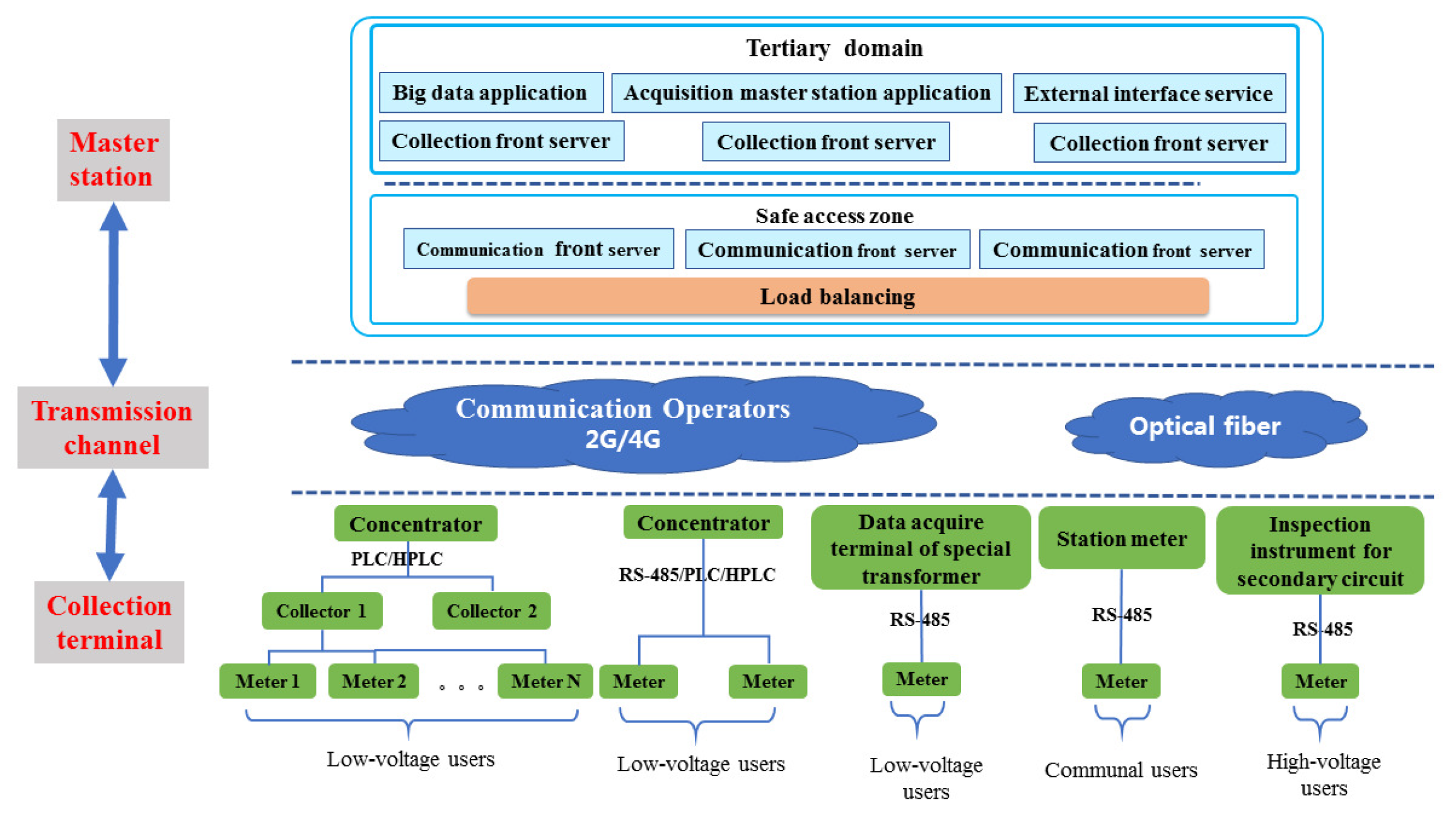
As shown in Figure 1, the electricity consumption information collection system is mainly composed of three parts: the system master station, the transmission channel and the collection terminal. As the central nervous system, the main station of the system is highly functional. It can transmit commands, effectively analyze terminal management and data and realize system and external interface maintenance. The transmission channel is used as a medium to connect the master station and the electric energy information collection terminal. The collection terminal, as the most important part of the electricity consumption information collection system, provides a data basis for electric energy analysis and power grid management. The collection terminal consists of collection equipment and electronic energy meters (i.e., smart meters). The data collected includes (1) power data such as base codes, increments, tariffs and electricity; (2) load data such as voltage, current, active power and reactive power; and (3) terminal working condition data. Moreover, the command issued by the master station is executed at the same time to complete the corresponding control function.
The collection device layer belongs to the power collection terminal, which is mainly used to collect and detect the data of the power meter, including the collection terminal and the power meter. The collection terminal collects the data of the electric energy meter and uploads it to the main station layer. The local communication between the collection terminal and electric meter mainly includes the power line carrier and RS-485 line mode. Among them, the carrier includes narrowband PLC(Power line communication) carrier and HPLC(High-speed power line communication) carrier. The RS-485 method is mainly used for special transformer users, photovoltaic users, general meters of the station area and medium-volume users of 50 kw and above. The carrier mode is mainly used for users with low voltage below 50 kw. In terms of communication efficiency and stability, RS-485 mode > HPLC high-speed carrier > narrowband PLC carrier.
The electricity consumption with uncertainty and strong nonlinearity varies with multiple factors including the weather, subjective preference and the change of electric equipment. It is difficult to accurately predict and recover the lost data only, depending on users’ own historical measurement data. How to recover measurement data according to their characteristics is the critical problem to be solved.
There are various kinds of users in the power grid, including ordinary residents, factories, shopping malls and so on. Although the matrix decomposition method can speed up the algorithm, larger calculation errors would be brought in if the eigenvalues with the same dimension were used to describe different user types. As a result, it is very difficult to eliminate the effects of heterogeneous users on the accuracy of recovered data.
The collaborative filtering algorithm [35] can improve the recovery accuracy of missing data in electric energy metering. At the same time, there is a great number of users in the power grid. Finding out the collaborative targets from huge user groups as quickly as possible is another important problem we are facing urgently to be solved.
2.2. Mathematical Model
The user set in the power grid is represented as , in which is the i-th user and M is the number of users. is the set of sampling moments for electric energy metering, where the j-th sampling moment is displayed as and the total number of samples for each user is shown as N. means the measurement data of the i-th user at the time , and its estimated value is referred to as . The measurement data of electricity users are shown chronologically in Table 1.
Here, is used to denote the Boolean state matrix, in which the value is set to 0 if the metering data is missing and 1 for others. The element in W is defined as Equation (1).
Suppose that the matrix is a matrix to be decomposed that contains a missing item and can be approximated as the multiplication of two matrices, as shown in Equation (2):
where and are two low-rank matrices and k represents the characteristic dimension. Each row of the eigenmatrix A represents the eigenvector of each user. In contrast, each row in the eigenmatrix B of the time series represents the feature vector of the current sampling moment.
3. Collaborative Fitting Algorithm
In this section, we first introduce the model and then describe its components. Afterwards, we provide an explanation of the loss function and optimizer parameters applied in the model.
3.1. ALS Matrix Decomposition
Currently, there are two commonly used matrix decomposition algorithms, namely singular value decomposition (SVD) and alternating least-squares decomposition (ALS). In SVD, the matrix decomposition operation can be executed as far as the missing values in the matrix are complemented using the weighted average method in advance. This makes the algorithm complexity of SVD higher. By contrast, ALS has relatively low complexity. It expresses data features through a set of low-dimensional cryptic meaning factors from a global perspective and then recovers the missing items in the matrix.
In order to obtain the submatrices A and B after matrix decomposition, the loss function is defined as Equation (4).
Furthermore, a generalization function is introduced to prevent over-fitting of the data. Equation (4) after being modified is shown as Equation (5):
where is the generalization function, and the generalization degree of data fitting can be controlled by adjusting the generalization factor .
Attributed to the difference between the estimated matrix and actual matrix, the loss function should be minimized to make the estimated values closer to the real data as soon as possible. According to the principle of least-squares, if matrix B is known, Equation (5) would take the derivative of any element in matrix A.
Let
then
where and are the i-th row of the matrix X and W, respectively. represents the d-th column of matrix B.
Suppose that represent a matrix composed of k matrixes and E is a identity matrix, then
In the same way, if the matrix A is known, one can obtain
where represents a matrix composed of k column vector .
3.2. Theoretical Derivation
Suppose that the matrix is a matrix to be decomposed that contains a missing item and can be approximated as the multiplication of two matrices A and B. Then, assume , so we can obtain the following theorem.
Theorem 1.
The smaller the value of the matrix rank r, the smaller the information loss in the matrix decomposition process. When r is close to 1, the loss function C approach 0, i.e.,
Proof.
For the matrix , it can be rewritten as the sum of two specified matrices. Hence, the bi-decomposition can be defined as follows:
where X is the matrix to be decomposed, and and are the basis matrix and difference matrix with the same dimension as X, respectively. At the same time, the rank of the base matrix is restricted to 1.
We carry out the singular value decomposition on the basis matrix . Then, SVD has the following form of factorization.
where U is a unitary matrix of order ; , the conjugate transpose of V, is a unitary matrix of order . is a positive semi-definite order diagonal matrix; the element on the diagonal of is the singular value of .
Since the rank of the base matrix is restricted to 1 in advance, it is clear that except for one singular value, the other singular values are all equal to 0. Suppose the first singular value is nonzero, then the diagonal matrix can be represented as
According to the definition of matrix rank, its value represents the scope of the feature space expanded by the singular vectors. It can be seen from the meaning of singular values that the magnitude determines the importance of the corresponding singular vector in the entire feature space, that is, how much feature information it contains. The larger the value is, the more characteristic information it contains, and the more important it is. Hence, the information hidden behind these higher singular values should be reserved when the dimensionality reduction is carried out on the matrix to be factorized.
From the discussion above, we notice that all the feature information in is related with one special vector—the eigenvector for the singular value.
Among various data dimensionality reduction algorithms for matrices, Principal Component Analysis (PCA) is a very commonly used method. It uses an orthogonal transformation to transform the original random vector whose components are related to a new random vector whose components are not related. Geometrically the original coordinate system is represented as transforming into a new orthogonal coordinate system. Calculate the eigenvalues of the matrix after transformation and compare their sizes. The large eigenvalues are retained, and the rest smaller eigenvalues are discarded. The matrix is reconstructed based on the eigenvectors corresponding to those reserved large eigenvalues. In regards to PCA, the information loss is decided by the smaller eigenvalues discarded. The smaller the proportion of these eigenvalues in all eigenvalues is, the less information loss is.
Since , all the feature information in is contained in the feature space expanded by the eigenvector for . Hence, the new extracted matrix would maintain all the information unchanged, and no information is lost if the PCA is conducted on and only one eigenvalue is selected. As a result, the truest result and the highest accuracy would be achieved when the basis matrix is utilized for data fitting and recovery.
As mentioned above, and would not lose any information after PCA. Thus, the information loss will happen to the difference matrix when PCA is carried out on the matrix X to be decomposed.
To sum up, plays the most vital role in data fitting and recovery and determines the accuracy of the fitting. When , . In other words, the limit
is reasonable, and the theorem is established. □
3.3. Nearest Neighbor Algorithm
From Equations (3) and (4) in the ALS algorithm, it can be seen that the loss function of the recovery matrix is closely related to the eigenvalue dimension. The characteristic dimensions vary for different user types. If the characteristic dimension chosen in the extracting period is identical for all users during matrix decomposition, the error will become larger and the data fitting accuracy will deteriorate consequently. Therefore, it is vital to decrease the errors caused by inconsistent feature dimensions as much as possible to improve the accuracy of data recovery. At the same time, the matrix decomposition algorithm with high dimensions also has higher computational complexity. As a result, the data of similar users should be used for collaborative fitting to reduce the algorithm complexity and realize the recovery of missing measurement data.
The nearest neighbor algorithm aims to find out the most similar co-users for one specific user, and the simplest way to implement is a traversal search. However, the method will take a lot of computing time when there is a large amount of power grid user data. Since the number of users in the power grid is much larger than the dimension of electric energy metering data, the rapid search among nearest-neighbor users can be promoted depending on the data model with tree structure.
The binomial tree model is established upon the accurate historical data of electric energy measurement. The dimension N is consistent with the historical sampling times. Let be the metering data of the user . The nearest neighbor search algorithm is elaborated as follows:
Step 1: Construct the root node.
Here, is viewed as the reference axis. Then, the median of all users’ coordinates on the reference axis calculated in Equation (9) is considered as the segmentation point, and the user nearest to the median is selected as the root node.
Thus, the measurement data are divided into left and right sub-regions. The right one corresponds to the region whose coordinate is larger than the segmentation point. In contrast, the left one correspond to the region whose coordinate is smaller than the segmentation point.
Step 2: Construct the child node repeatedly.
For a child node with the depth h, is selected as the reference axis. The root node for each sub-region is constructed according to Step 1. Then, the root node is taken as the child node of its parent node until the sub-region does not contain any user data. The parameter p is obtained using Equation (10).
Step 3: Nearest neighbor search.
For a given target user, the leaf node containing the user is first found in the tree structure. Then, the parent node is successively backtracked to find its nearest point in Euclidean distance.
3.4. Data Recovery Algorithm
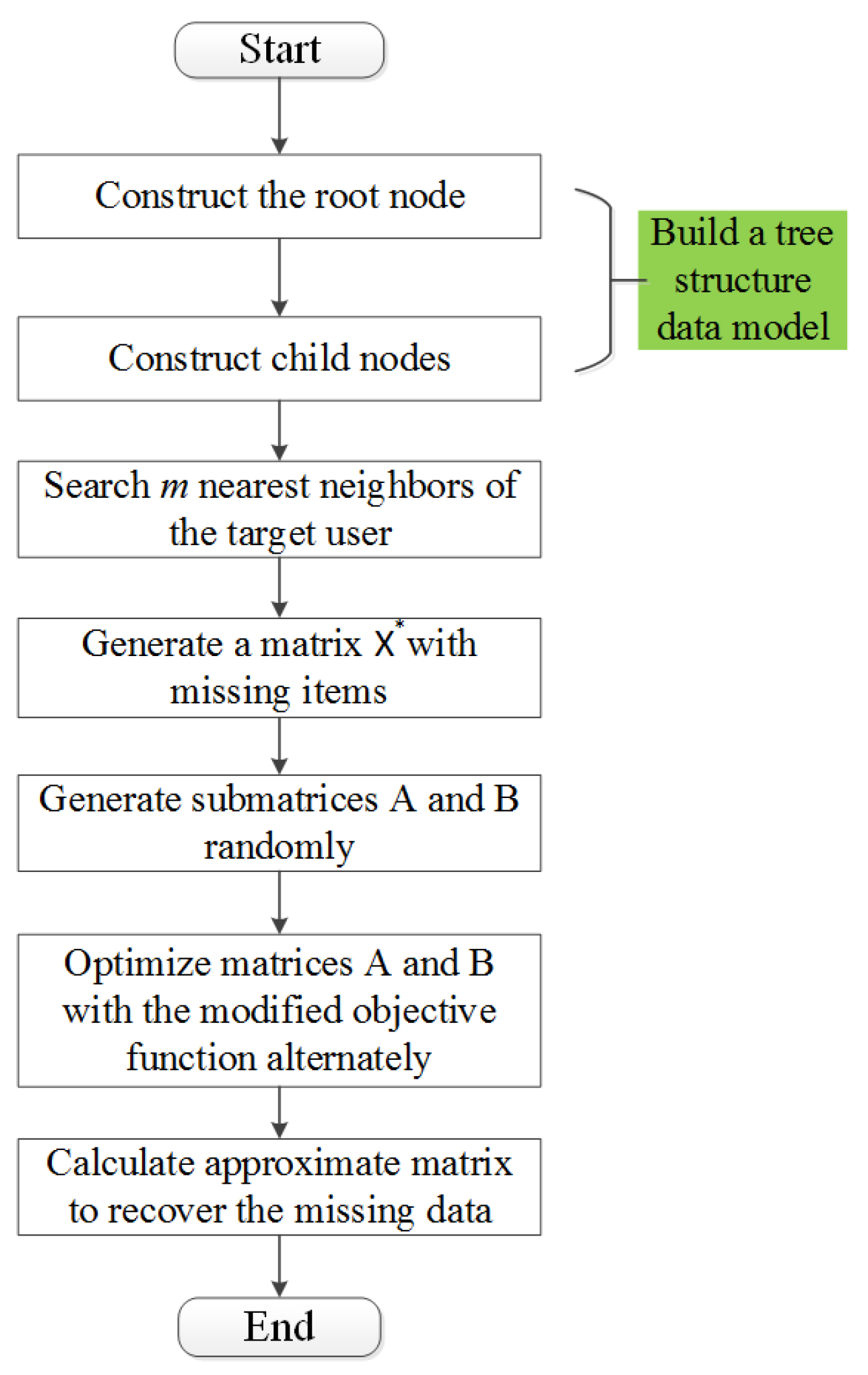
Suppose that the data of m() users are required for collaborative fitting when recovering the missing data of one user. The flow of the data recovery algorithm proposed in this paper is shown in Figure 2.
If the traversal search is adopted in the nearest neighbor search, its complexity is . In contrast, the complexity is when the binomial tree search is chosen. It is obviously that the nearest neighbor algorithm raised in this paper speeds up the search. When the matrix is factorized by the ALS decomposition algorithm, its dimension is reduced from to . This not only improves the data recovery accuracy but also simplifies the calculation parameters and further reduces the algorithm complexity.
4. Numerical Simulation and Analysis
In order to further verify the effectiveness of the proposed data recovery algorithm, comparisons with other two kinds of fitting algorithms are conducted and analyzed on a data set obtained from a power metering center. The experiments are implemented in Matlab 2017. In the dataset, and . There are about 658 missing data items that not only affected the normal accounting business but also caused complaints from users. The measurement data of test user extracted in the simulation verification was shown in Table 2.
4.1. Comparative Analysis of Fitting Accuracy
Firstly, the polynomial fitting algorithm and power function-fitting algorithm are chosen to fit the time series to evaluate their performance. Here, a simple polynomial model, quadratic polynomial model and triple-order polynomial model are applied for the polynomial fitting algorithm. The corresponding experimental results are shown in the following three pictures. Besides the fitting curve, the equation and the indexes for fitting accuracy are also provided for a better analysis of the fitting results. In this paper, those indexes include the sum of the squared errors (), root mean squared error (), coefficient of determination () and its adjusted value (). Known from the definitions, the smaller the values of and are, the more accurate the fitting results are. Conversely, the closer to 1 the values of and are, the more similar to the actual curve the fitted curve is.
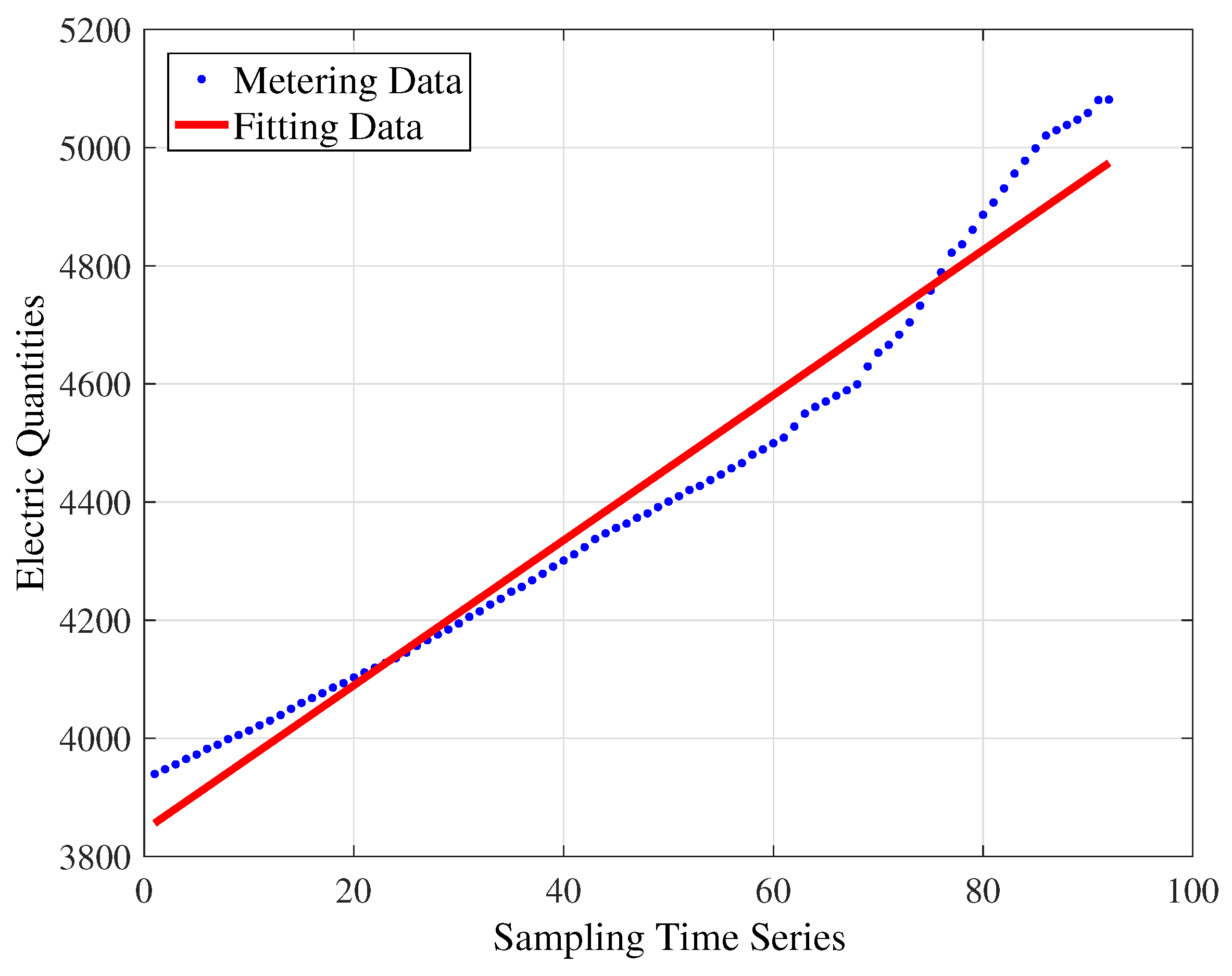
For the simple polynomial model shown in Figure 3, the fitting equation achieved is . The values of , , and are 33,410, 60.93, 0.9670 and 0.9666, respectively.
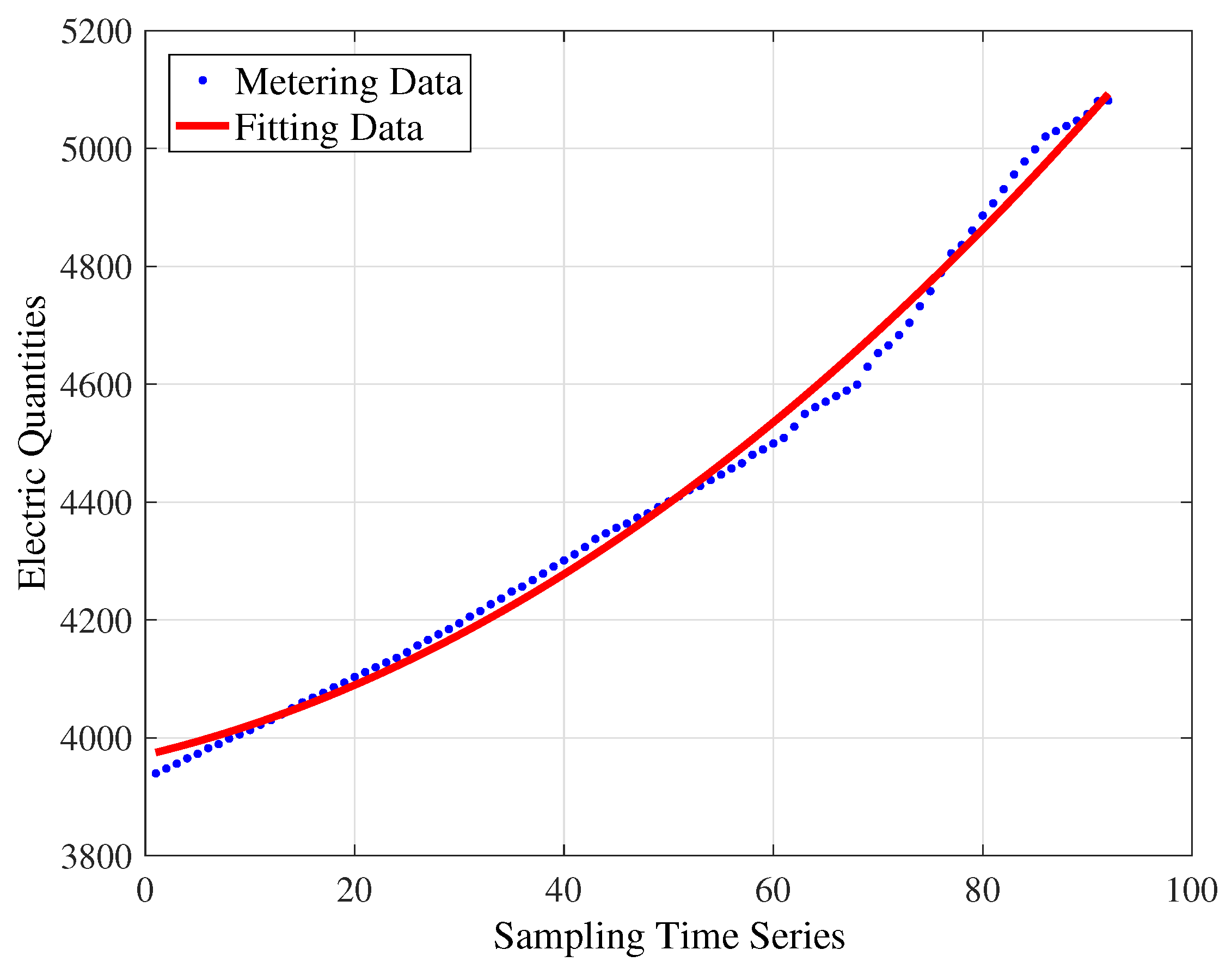
For the quadratic polynomial model shown in Figure 4, the fitting equation achieved is . The values of , , and are 57,760, 25.48, 0.9943 and 0.9942, respectively.
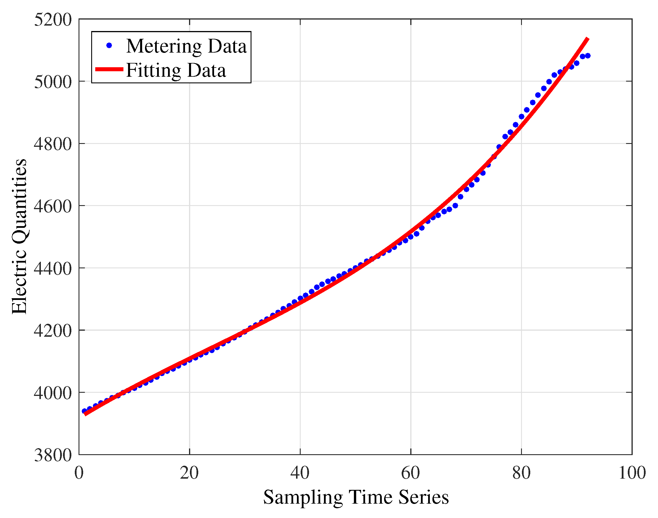
For the triple-order polynomial model shown in Figure 5, the fitting equation achieved is . The values of , , and are 25,600, 17.06, 0.9975 and 0.9974, respectively.
Meanwhile, the first-order power function and second-order power function are adopted in the power function-fitting algorithm. The fitting curves are revealed in Figure 6 and Figure 7, and the specific fitting parameters are offered following the pictures.
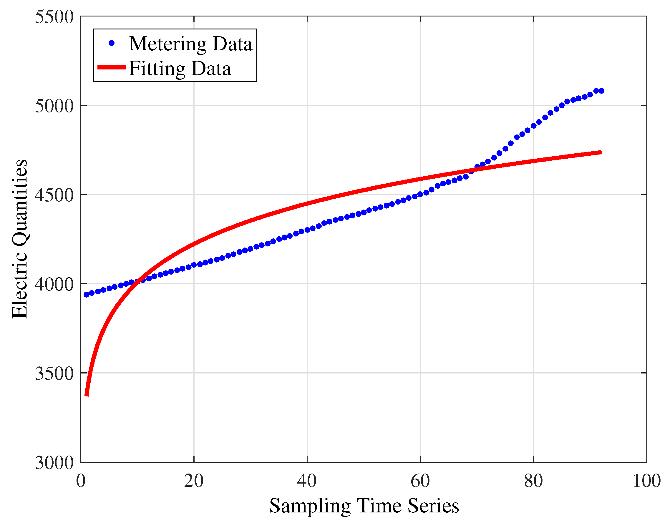
For the first-order power function model shown in Figure 6, the fitting equation achieved is . The values of , , and are 2,736,000, 174.4, 0.7295 and 0.7265, respectively.
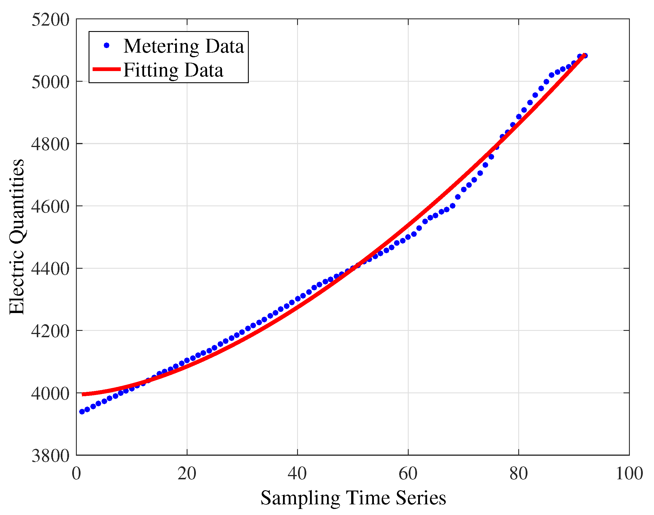
For the second-order power function model shown in Figure 7, the fitting equation achieved is . The values of , , and are 74,170, 28.87, 0.9927 and 0.9925, respectively.
Based on the analysis of those fitting results, it can be known that the polynomial fitting algorithm and power function-fitting algorithm cannot obtain the ideal fitting accuracy. Then, the simulation experiment on the matrix factorization method is conducted to verify its superiority relative to the above two algorithms. The original ALS algorithm is selected for the decomposition, and the embedded parameters are set as , .
Two sets of experiments on the matrix factorization method are carried out in which one is with the collaborative information and the other is not. Figure 8 displays the curve fitted by the alternating least-squares algorithm without the collaborative information. Moreover, the values of , , and are 53,809.82, 24.1844, 0.9979 and 0.9978, respectively. The result is as good as that obtained by the polynomial fitting algorithm with triple-order polynomial model and is better that those for the other four cases.
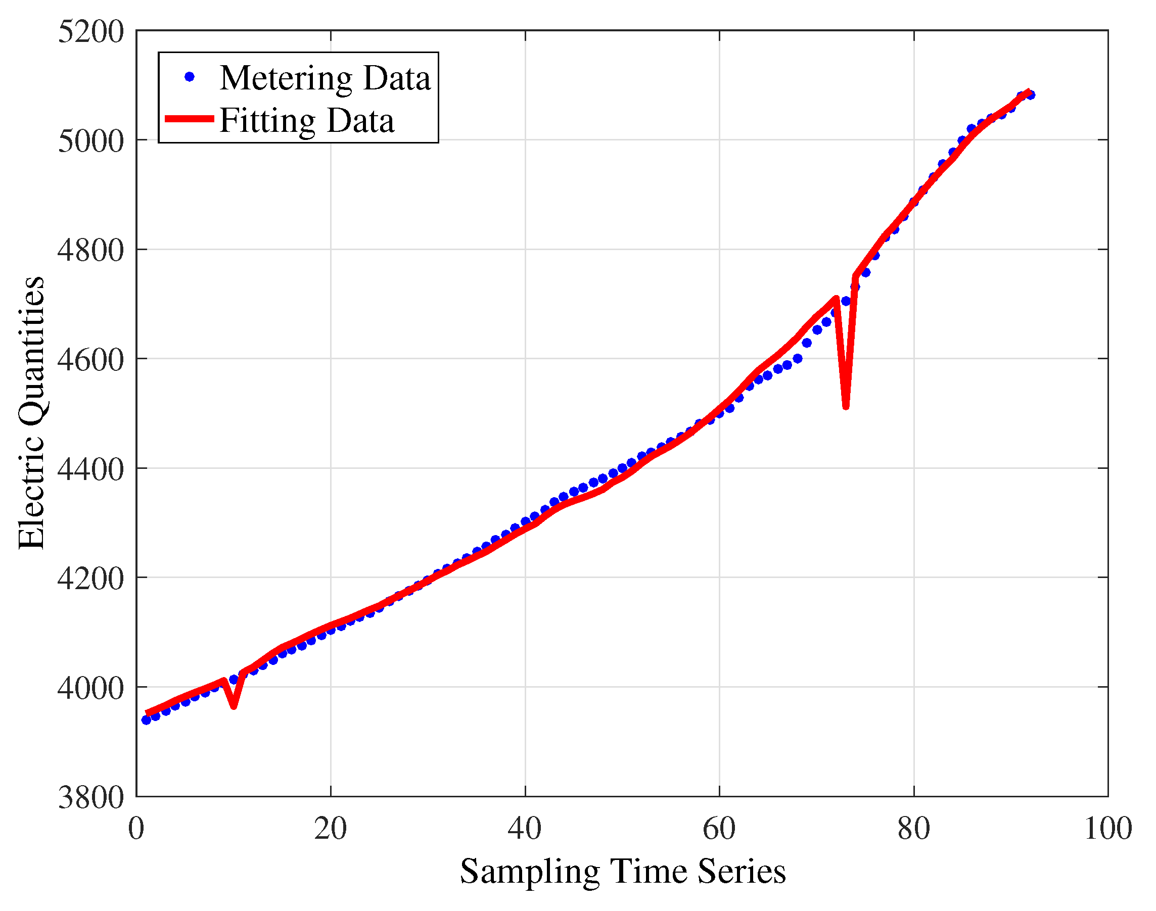
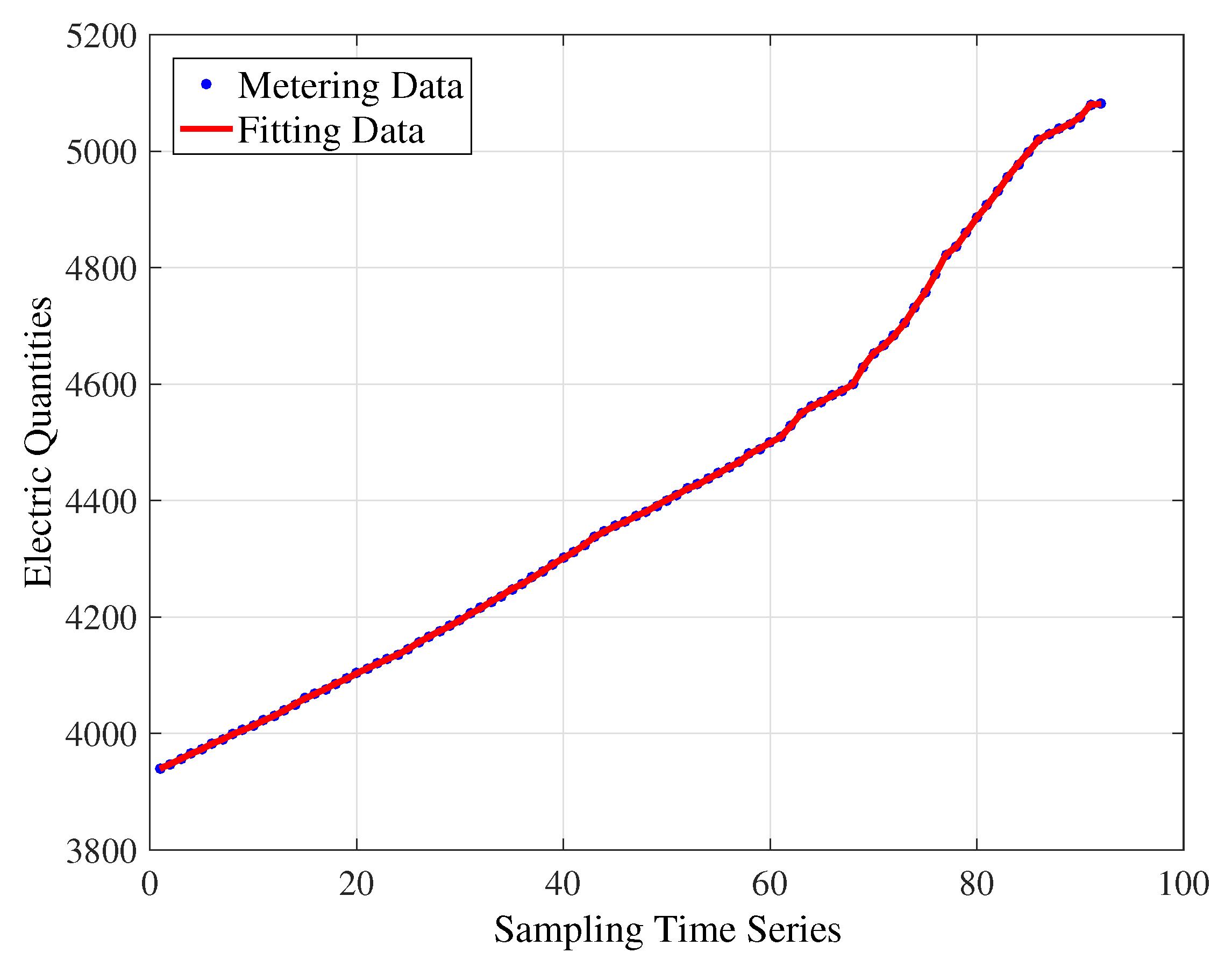
Next, we will study how much influence the collaborative information has on the matrix factorization. The collaborative information is joined in the alternating least-squares algorithm, and thus, the fitting curve obtained is shown in Figure 9.
As can be seen in the figure, the fitting curve is almost completely coincident with the original curve. In particular, the parameters for measuring the goodness of fit are calculated, where , , , . These index values are significantly better than the others. This means the ALS algorithm with collaboration has the best fitting accuracy, and the collaborative information is obviously beneficial to the feature extraction. The conclusion is also clearly in accord with the comparison in Table 3.
Observing the simulation results, it can be seen from Table 3 that because the time series data of the electric energy measurement has strong nonlinearity, the error between the original data and the predicted data recovered by the polynomial fitting algorithm and the power function-fitting algorithm is relatively large when the time series is used as the dependent variable. Their goodness of fit is not as good as the algorithm based on matrix factorization. Among them, the improved matrix factorization algorithm based on user collaboration proposed in this paper has the highest goodness of fit. The improved collaborative fitting ALS algorithm is available with higher recovery accuracy. This further illustrates that similar users have a closer relationship between the electric energy measurement values through implicit semantics. In addition, it is more convincing and reliable in real life to fill up the missing data of power consumption by employing the nearest neighbor user’s electric energy measurement than the time-series-based fitting algorithm.
4.2. Evaluation of Accuracy on Predicting the Missing Data
As known to all, the final purpose of curve fitting is to predict the unknown data on the function. Here, the test user with 92 sampling points serves as an example. Suppose that the top 91 points are determined, and the last one is missing when collected. Now, we predict this point through the function fitted on those undoubted 91 points. The simulation results, including the fitted function, are shown in Table 4, and the forecast values are presented to determine whether it is accurate as well.
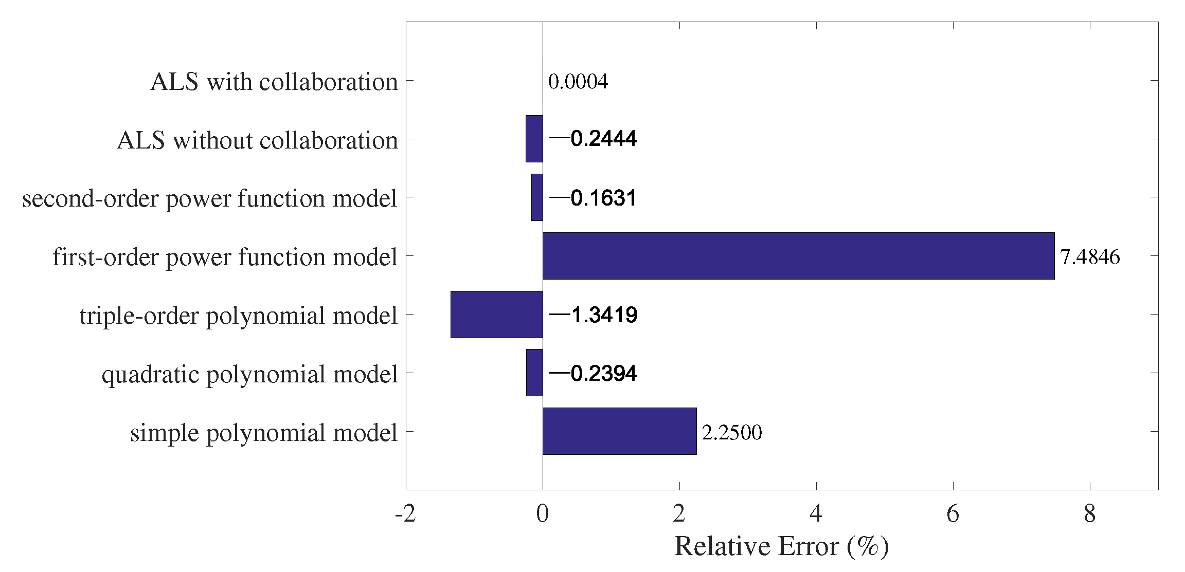
As can be seen from Table 4, the actual value of the last sampling point is 5081.21. The relative errors between that and each predicted value are calculated and drawn in Figure 10. It can be seen that the predicted values of all methods, except for the simple polynomial model and the first-order power function model, are larger than the actual value. The ALS algorithm with collaboration has a far smaller error than others, followed by the second-order power function model. The quadratic polynomial model shares a similar result with the ALS algorithm without collaboration. The other three methods obtain very poor performance compared to the above four methods and are not suitable for predicting the data missed.
Since the relative error between the actual value and that predicted by the ALS algorithm with collaboration, which is , is very close to 0, the predicted value can be used as the true value of the missed data reasonably and credibly. As a result, the method proposed in this paper is particularly suitable for predicting the missing data and would obtain results that are more accurate.
In actual engineering applications, predicting the missing data instead of recollecting manually can effectively reduce manual on-site operations and save labor costs. Therefore, the improved ALS algorithm has higher value of application and promotion.
4.3. Parametric Analysis of the Proposed Algorithm
As known to all, there are two key parameters to be set in the proposed ALS algorithm with collaboration: the eigenvalue dimension (k) and generalization factor (). The accuracy of the matrix factorization algorithm largely depends on those two parameters, and how to determine them is a difficult but vital problem in a variety of applications. A detailed study is executed to investigate the influence of these two parameters on the performance of the improved ALS algorithm. Experiments are conducted on three set values for the eigenvalue dimension (k) and generalization factor (), respectively.
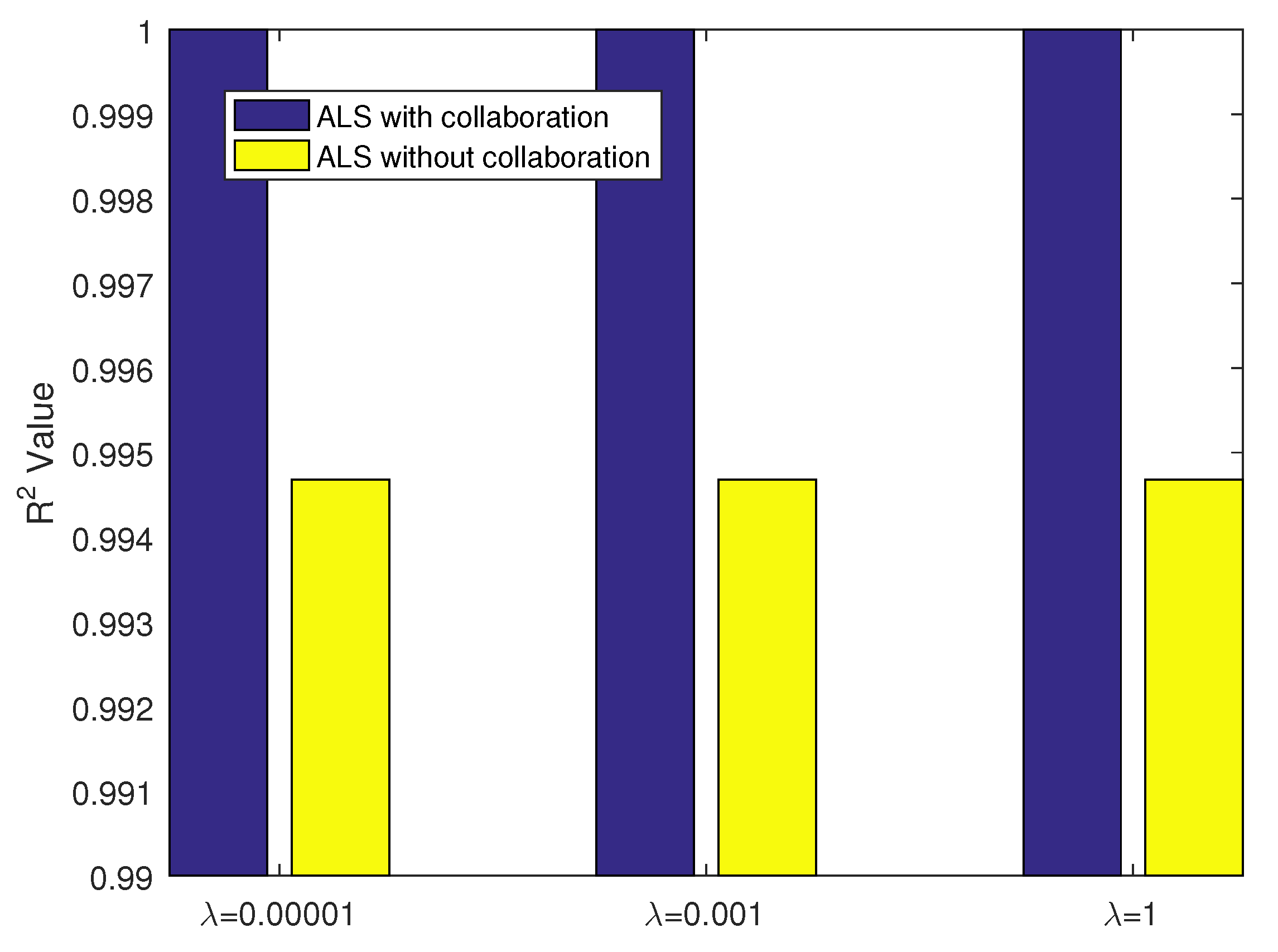
First, we investigate the impact of the parameter by keeping the parameter k unchanged. Here, the value of k is set to 2 and , the most representative index to measure the fitting accuracy, is selected for comparison. When the generalization factor , the value change trend is shown in Figure 11.
As can be seen from Figure 11, no matter how the parameter changes, the values obtained by the ALS algorithm combined with the method proposed in this paper are larger than those of the original ALS algorithm without collaboration. It means that the fusion of collaboration information is beneficial to improve the fitting accuracy of ALS. With regard to different parameter values, the corresponding values are almost unchanged and equal to each other. In other words, the variation of parameter has no effect on the performance of both the original ALS algorithm and the proposed ALS algorithm with collaboration. Since the parameter is designed to prevent the algorithm overfitting, the overfitting will not happen in the improved algorithm proposed in this paper.
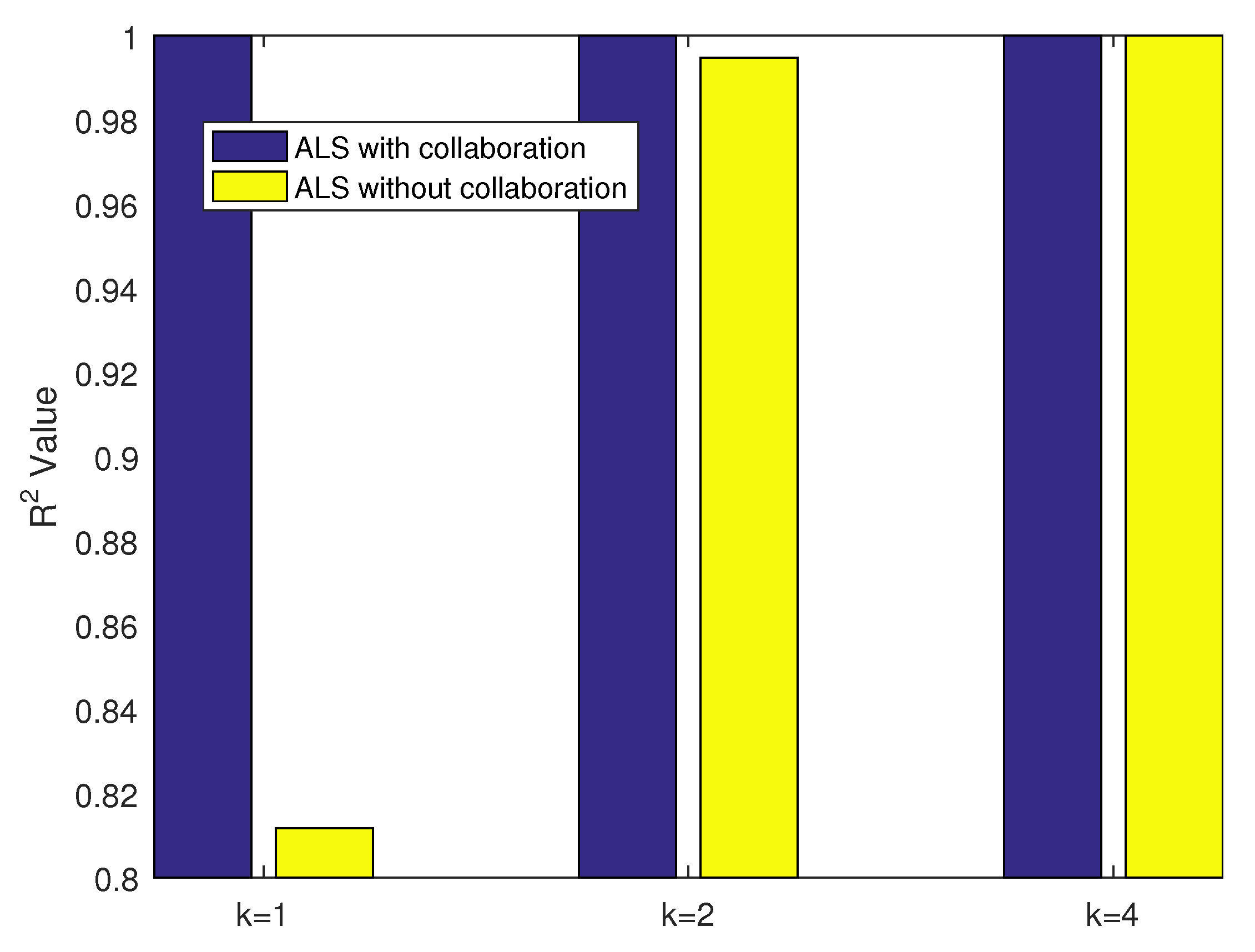
Moreover, the impact of the parameter k is studied when the parameter is set as 0.01. The values 1, 2 and 4 are chosen for the parameter k, and the fitting results are displayed in Figure 12.
It is obvious that the proposed algorithm is superior to the unimproved algorithm in terms of fitting accuracy. Focusing on the results of the original ALS algorithm without collaboration, the values are obviously changing with the alteration of the parameter k. In detail, when k is equal to 4, the value is 0.999, which is 1.23 times the value (0.812) obtained with . Different values will result in a completely unpredictable fitting performance. This brings great difficulties for the researchers to find a suitable value when facing various problems. By contrast, with regard to the ALS algorithm with collaboration, all the values are extremely close to 1 for each value of parameter k. It indicates that the parameter k has scarcely influence the fitting performance. As a result, the burden of determining parameter k can be ignored, and better fitting performance will be achieved whether the dimension of the feature vector is known in advance or not.
To sum up, it is concluded that the proposed ALS algorithm with collaboration holds more accurate fitting performance and is not sensitive to neither the eigenvalue dimension (k) nor the generalization factor () relative to the original ALS algorithm. This enhances the stability of algorithm performance and reduces the burden of parameter adjustment.
5. Conclusions
In order to recover the missing value of electric energy measurement data quickly and efficiently, this paper proposes a cooperative fitting algorithm based on the binary tree search algorithm and the matrix decomposition algorithm. Firstly, the tree structure of historical user data is established, and then the user groups adjacent to the missing user are obtained. Finally, the missing data are recovered using the alternating least-squares matrix decomposition algorithm. This method has high reliability and accuracy in solving the missing data problem.
When looking for the similarity of users, this paper only uses the dimension data of electricity consumption, and more dimensions are needed to describe the user portrait more accurately. In the future, the similarity among users will be analyzed by considering features other than power measurement data. In real life, the feature dimensions of users are relatively complex. Advanced big data technology can be used to conduct in-depth mining of user features and then analyze the principal components and correlation degree of high-dimension features. Through engineering demonstration, improving data fitting accuracy can save operation cost, and promoting this method to engineering applications is also the focus of the next step.
Author Contributions
Methodology, Y.X. and Z.Z.; software, S.X. and X.K.; validation, Y.X., Z.Z., S.X. and C.J.; formal analysis, Y.X., Z.Z., S.X. and C.J.; writing—original draft preparation, Y.X. and X.K.; writing—review and editing, X.K.; project administration, Y.X. and X.K. All authors have read and agreed to the published version of the manuscript.
Funding
This research received no external funding.
Institutional Review Board Statement
Not applicable.
Informed Consent Statement
Not applicable.
Data Availability Statement
All data are presented in the paper.
Conflicts of Interest
The authors declare no conflict of interest.
Abbreviations
The following abbreviations are used in this manuscript:
| MF | matrix factorization |
| ALS | alternating least-squares |
| CF | collaborative filtering |
| PLC | power line communication |
| HPLC | high-speed power line communication |
| SVD | singular value decomposition |
| PCA | principal component analysis |
| SSE | sum of the squared errors |
| RMSE | root mean squared error |
References
- Teng, X.; Lu, D.; Chiu, Y. Emission reduction and energy performance improvement with different regional treatment intensity in China. Energies 2019, 12, 237. [Google Scholar] [CrossRef] [Green Version]
- Praditia, T.; Walser, T.; Oladyshkin, S.; Nowak, W. Improving thermochemical energy storage dynamics forecast with physics-inspired neural network architecture. Energies 2020, 13, 3873. [Google Scholar] [CrossRef]
- Li, C.; Ding, Z.; Yi, J.; Lv, Y.; Zhang, G. Deep belief network based hybrid model for building energy consumption prediction. Energies 2018, 11, 242. [Google Scholar] [CrossRef] [Green Version]
- Moreno Escobar, J.J.; Morales Matamoros, O.; Tejeida Padilla, R.; Lina Reyes, I.; Quintana Espinosa, H. A Comprehensive Review on Smart Grids: Challenges and Opportunities. Sensors 2021, 21, 6978. [Google Scholar] [CrossRef] [PubMed]
- González, I.; Calderón, A.J.; Portalo, J.M. Innovative Multi-Layered Architecture for Heterogeneous Automation and Monitoring Systems: Application Case of a Photovoltaic Smart Microgrid. Sustainability 2021, 13, 2234. [Google Scholar] [CrossRef]
- Schmeck, H.; Lösch, M.; Növer, R.; Ronczka, M.; Schmeck, H. Smart Meter Gateways: Options for a BSI-compliant integration of energy management systems. Appl. Sci. 2019, 9, 1634. [Google Scholar]
- Jones, K.D.; Pal, A.; Thorp, J.S. Methodology for performing synchrophasor data conditioning and validation. IEEE Trans. Power Syst. 2015, 30, 1121–1130. [Google Scholar] [CrossRef]
- Ding, Z.; Mei, G.; Cuomo, S.; Li, Y.; Xu, N. Comparison of estimating missing values in iot time series data using different interpolation algorithms. Int. J. Parallel Prog. 2020, 48, 534–548. [Google Scholar] [CrossRef]
- Deng, W.; Guo, Y.; Liu, J.; Li, Y.; Liu, D.; Zhu, L. A missing power data filling method based on improved random forest algorithm. Chin. J. Elect. Eng. 2019, 5, 33–39. [Google Scholar] [CrossRef]
- Pan, L.; Li, J. K-nearest neighbor based missing data estimation algorithm in wireless sensor networks. Wirel. Sens. Netw. 2010, 2, 115–122. [Google Scholar] [CrossRef] [Green Version]
- Chai, X.; Gu, H.; Li, F.; Duan, H.; Hu, X.; Lin, K. Deep learning for irregularly and regularly missing data reconstruction. Sci. Rep. 2020, 10, 1–18. [Google Scholar] [CrossRef] [PubMed]
- James, J.Q.; Hill, D.J.; Li, V.O.; Hou, Y. Synchrophasor recovery and prediction: A graph-based deep learning approach. IEEE Internet Things 2019, 6, 7348–7359. [Google Scholar]
- Feng, L.; Huang, J.; Shu, S.; An, B. Regularized Matrix Factorization for Multilabel Learning with Missing Labels. IEEE Trans. Cybern. 2020, 1–12. [Google Scholar] [CrossRef] [PubMed]
- Konstantinopoulos, S.; De Mijolla, G.M.; Chow, J.H.; Lev-Ari, H.; Wang, M. Synchrophasor missing data recovery via data-driven filtering. IEEE Trans. Smart Grid 2020, 11, 4321–4330. [Google Scholar] [CrossRef]
- Yang, C.; Wang, Z.J.; Liu, Z.H.; Yu, N.N. Research and Application of Cloud Manufacturing Service Platform for Crane. J. Syst. Simul. 2017, 29, 1351–1358. [Google Scholar]
- Yu, N.N.; Wang, Z.J. Research on Collaborative Filtering Algorithm Based on Spark. Syst. Simul. Technol. 2016, 12, 40–45. [Google Scholar]
- Yang, Z.W.; Liu, H.; Bi, T.S.; Yang, Q.X. A PMU Data Recovery Method Based on Singular Value Decomposition. Proc. CSEE 2020, 40, 812–821. [Google Scholar]
- Frenich, A.G.; Galera, M.M.; Vidal, J.M.; Massart, D.L.; Torres-Lapasió, J.R.; De Braekeleer, K.; Wang, J.-H.; Hopke, P.K. Resolution of multicomponent peaks by orthogonal projection approach, positive matrix factorization and alternating least squares. Anal. Chim. Acta 2000, 411, 145–155. [Google Scholar] [CrossRef]
- Kim, H.; Park, H. Nonnegative matrix factorization based on alternating nonnegativity constrained least squares and active set method. SIAM J. Matrix Anal. Appl. 2008, 30, 713–730. [Google Scholar] [CrossRef]
- Zhao, K.; Zhang, Z. Successively alternate least square for low-rank matrix factorization with bounded missing data. Comput. Vis. Image Underst. 2010, 114, 1084–1096. [Google Scholar] [CrossRef]
- Liu, H.; Li, X.; Zheng, X. Solving non-negative matrix factorization by alternating least squares with a modified strategy. Data Min. Knowl. Discov. 2013, 26, 435–451. [Google Scholar] [CrossRef]
- Lee, S.; Pang, H.S. Multichannel non-negative matrix factorisation based on alternating least squares for audio source separation system. Electron. Lett. 2015, 51, 197–198. [Google Scholar] [CrossRef]
- Giampouras, P.V.; Rontogiannis, A.A.; Koutroumbas, K.D. Alternating iteratively reweighted least squares minimization for low-rank matrix factorization. IEEE Trans. Signal Proces. 2018, 67, 490–503. [Google Scholar] [CrossRef]
- Chen, J.; Fang, J.; Liu, W.; Tang, T.; Yang, C. clmf: A fine-grained and portable alternating least squares algorithm for parallel matrix factorization. Future Gener. Comput. Syst. 2020, 108, 1192–1205. [Google Scholar] [CrossRef] [Green Version]
- Belachew, M.T.; Del Buono, N. Hybrid projective nonnegative matrix factorization based on α-divergence and the alternating least squares algorithm. Appl. Math. Comput. 2020, 369, 124825. [Google Scholar] [CrossRef]
- Zhu, W.; Huang, K.; Xiao, X.; Liao, B.; Yao, Y.; Wu, F.X. ALSBMF: Predicting lncRNA-disease associations by alternating least squares based on matrix factorization. IEEE Access 2020, 8, 26190–26198. [Google Scholar] [CrossRef]
- Chen, J.; Fang, J.; Liu, W.; Yang, C. BALS: Blocked Alternating Least Squares for Parallel Sparse Matrix Factorization on GPUs. IEEE Trans. Parallel Distrib. Syst. 2021, 32, 2291–2302. [Google Scholar] [CrossRef]
- Luo, X.; Zhou, M.; Xia, Y.; Zhu, Q. An efficient non-negative matrix-factorization-based approach to collaborative filtering for recommender systems. IEEE Trans. Ind. Inform. 2014, 10, 1273–1284. [Google Scholar]
- Li, C.; He, K. CBMR: An optimized MapReduce for item-based collaborative filtering recommendation algorithm with empirical analysis. Concurr. Comput. Pract. Exp. 2017, 29, e4092. [Google Scholar] [CrossRef]
- Hernando, A.; Bobadilla, J.; Ortega, F. A non negative matrix factorization for collaborative filtering recommender systems based on a Bayesian probabilistic model. Knowl.-Based Syst. 2016, 97, 188–202. [Google Scholar] [CrossRef]
- Polato, M.; Aiolli, F. Exploiting sparsity to build efficient kernel based collaborative filtering for top-N item recommendation. Neurocomputing 2017, 268, 17–26. [Google Scholar] [CrossRef] [Green Version]
- Polato, M.; Aiolli, F. Boolean kernels for collaborative filtering in top-N item recommendation. Neurocomputing 2018, 286, 214–225. [Google Scholar] [CrossRef] [Green Version]
- Singh, P.K.; Sinha, M.; Das, S.; Choudhury, P. Enhancing recommendation accuracy of item-based collaborative filtering using Bhattacharyya coefficient and most similar item. Appl. Intell. 2020, 50, 4708–4731. [Google Scholar] [CrossRef]
- Guo, J.; Deng, J.; Ran, X.; Wang, Y.; Jin, H. An efficient and accurate recommendation strategy using degree classification criteria for item-based collaborative filtering. Expert Syst. Appl. 2021, 164, 113756. [Google Scholar] [CrossRef]
- Chen, B.W.; Ye, W.C. Low-Error Data Recovery Based on Collaborative Filtering with Nonlinear Inequality Constraints for Manufacturing Processes. IEEE Trans. Autom. Sci. Eng. 2020, 18, 1602–1614. [Google Scholar] [CrossRef]
Figure 1.
Block diagram of power consumption information collection system.

Figure 2.
Flow chart of data recovery algorithm.

Figure 3.
Simple polynomial model.

Figure 4.
Quadratic polynomial model.

Figure 5.
Triple-order polynomial model.

Figure 6.
First-order power function model.

Figure 7.
Second-order power function model.

Figure 8.
ALS without collaborative information.

Figure 9.
ALS with collaborative information.

Figure 10.
Relative errors between the predicted value and actual one.

Figure 11.
values obtained with different values.

Figure 12.
values obtained with different k values.


Table 1.
Time series data of electric energy measuring.
| t | t | ⋯ | t | ⋯ | t | |
|---|---|---|---|---|---|---|
| ⋯ | ⋯ | |||||
| ⋯ | ⋯ | |||||
| ⋮ | ⋮ | ⋮ | ⋱ | ⋮ | ⋱ | ⋮ |
| ⋯ | ⋯ | |||||
| ⋮ | ⋮ | ⋮ | ⋱ | ⋮ | ⋱ | ⋮ |
| ⋯ | ⋯ |
Table 2.
Electric energy measuring data of .
| 1 | 3939.61 | 32 | 4215.03 | 63 | 4549.69 |
| 2 | 3947.81 | 33 | 4226.53 | 64 | 4561.08 |
| 3 | 3956.14 | 34 | 4236.26 | 65 | 4570.32 |
| 4 | 3965.16 | 35 | 4248.23 | 66 | 4580.05 |
| 5 | 3972.68 | 36 | 4256.48 | 67 | 4589.09 |
| 6 | 3982.42 | 37 | 4267.51 | 68 | 4599.30 |
| 7 | 3989.32 | 38 | 4278.64 | 69 | 4629.58 |
| 8 | 3998.66 | 39 | 4290.64 | 70 | 4652.85 |
| 9 | 4005.65 | 40 | 4301.05 | 71 | 4666.04 |
| 10 | 4013.21 | 41 | 4311.43 | 72 | 4683.34 |
| 11 | 4022.14 | 42 | 4323.72 | 73 | 4704.18 |
| 12 | 4030.07 | 43 | 4337.50 | 74 | 4732.39 |
| 13 | 4039.54 | 44 | 4347.03 | 75 | 4757.79 |
| 14 | 4050.02 | 45 | 4356.21 | 76 | 4788.75 |
| 15 | 4060.08 | 46 | 4363.51 | 77 | 4822.12 |
| 16 | 4068.20 | 47 | 4373.38 | 78 | 4836.16 |
| 17 | 4076.40 | 48 | 4380.82 | 79 | 4860.81 |
| 18 | 4085.94 | 49 | 4391.47 | 80 | 4886.12 |
| 19 | 4093.54 | 50 | 4401.00 | 81 | 4906.98 |
| 20 | 4103.15 | 51 | 4410.03 | 82 | 4930.83 |
| 21 | 4111.57 | 52 | 4420.55 | 83 | 4955.92 |
| 22 | 4119.71 | 53 | 4427.32 | 84 | 4977.73 |
| 23 | 4127.77 | 54 | 4437.32 | 85 | 4998.52 |
| 24 | 4135.70 | 55 | 4446.60 | 86 | 5020.17 |
| 25 | 4145.17 | 56 | 4457.09 | 87 | 5029.46 |
| 26 | 4156.62 | 57 | 4465.80 | 88 | 5038.15 |
| 27 | 4166.12 | 58 | 4480.37 | 89 | 5047.21 |
| 28 | 4175.74 | 59 | 4489.21 | 90 | 5058.51 |
| 29 | 4184.39 | 60 | 4499.45 | 91 | 5080.32 |
| 30 | 4194.28 | 61 | 4508.99 | 92 | 5081.21 |
| 31 | 4205.72 | 62 | 4527.83 | — | — |
Table 3.
Comparison of the fitting indexes.
| Method | ||||
|---|---|---|---|---|
| simple polynomial model | 334,100 | 60.93 | 0.967 | 0.9666 |
| quadratic polynomial model | 57,760 | 25.48 | 0.9943 | 0.9942 |
| triple-order polynomial model | 25,600 | 17.06 | 0.9975 | 0.9974 |
| first-order power function model | 2,736,000 | 174.4 | 0.7295 | 0.7265 |
| second-order power function model | 74,170 | 28.87 | 0.9927 | 0.9925 |
| ALS without collaboration | 53,809.82 | 24.1844 | 0.9979 | 0.9978 |
| ALS with collaboration | 0.07979 | 0.02945 | 0.99993 | 0.99993 |
Table 4.
Fitting and predicting results.
| Method | Fitted Function | Predicted Value |
|---|---|---|
| simple polynomial | 4969.4 | |
| quadratic polynomial | 5093.404 | |
| triple-order polynomial | 5150.322 | |
| first-order power function | 4727.383 | |
| second-order power function | 5089.512 | |
| ALS without collaboration | - | 5093.66 |
| ALS with collaboration | - | 5081.19 |
Publisher’s Note: MDPI stays neutral with regard to jurisdictional claims in published maps and institutional affiliations. |
© 2022 by the authors. Licensee MDPI, Basel, Switzerland. This article is an open access article distributed under the terms and conditions of the Creative Commons Attribution (CC BY) license (https://creativecommons.org/licenses/by/4.0/).
Share and Cite
MDPI and ACS Style
Xu, Y.; Kong, X.; Zhu, Z.; Jiang, C.; Xiao, S. Recovery Algorithm of Power Metering Data Based on Collaborative Fitting. Energies 2022, 15, 1570. https://0-doi-org.brum.beds.ac.uk/10.3390/en15041570
AMA Style
Xu Y, Kong X, Zhu Z, Jiang C, Xiao S. Recovery Algorithm of Power Metering Data Based on Collaborative Fitting. Energies. 2022; 15(4):1570. https://0-doi-org.brum.beds.ac.uk/10.3390/en15041570
Chicago/Turabian StyleXu, Yukun, Xiangyong Kong, Zheng Zhu, Chao Jiang, and Shuang Xiao. 2022. "Recovery Algorithm of Power Metering Data Based on Collaborative Fitting" Energies 15, no. 4: 1570. https://0-doi-org.brum.beds.ac.uk/10.3390/en15041570
Note that from the first issue of 2016, this journal uses article numbers instead of page numbers. See further details here.