Article

Computational Analysis of Shear Banding in Simple Shear Flow of Viscoelastic Fluid-Based Nanofluids Subject to Exothermic Reactions

1
Department of Mathematics and Applied Mathematics, University of Cape Town, Cape Town 7701, South Africa
2
Centre for Research in Computational & Applied Mechanics, University of Cape Town, Cape Town 7701, South Africa
3
Centre for High Performance and Computing, Council for Scientific and Industrial Research, Cape Town 7700, South Africa
*
Author to whom correspondence should be addressed.
Submission received: 29 December 2021 / Revised: 15 January 2022 / Accepted: 18 January 2022 / Published: 25 February 2022

Abstract

:
We investigated the shear banding phenomena in the non-isothermal simple-shear flow of a viscoelastic-fluid-based nanofluid (VFBN) subject to exothermic reactions. The polymeric (viscoelastic) behavior of the VFBN was modeled via the Giesekus constitutive equation, with appropriate adjustments to incorporate both the non-isothermal and nanoparticle effects. Nahme-type laws were employed to describe the temperature dependence of the VFBN viscosities and relaxation times. The Arrhenius theory was used for the modeling and incorporation of exothermic reactions. The VFBN was modeled as a single-phase homogeneous-mixture and, hence, the effects of the nanoparticles were based on the volume fraction parameter. Efficient numerical schemes based on semi-implicit finite-difference-methods were employed in MATLAB for the computational solution of the governing systems of partial differential equations. The fundamental fluid-dynamical and thermodynamical phenomena, such as shear banding, thermal runaway, and heat transfer rate (HTR) enhancement, were explored under relevant conditions. Important novel results of industrial significance were observed and demonstrated. Firstly, under shear banding conditions of the Giesekus-type VFBN model, we observed remarkable HTR and Therm-C enhancement in the VFBN as compared to, say, NFBN. Specifically, the results demonstrate that the VFBN are less susceptible to thermal runaway than are NFBN. Additionally, the results illustrate that the reduced susceptibility of the Giesekus-type VFBN to the thermal runaway phenomena is further enhanced under shear banding conditions, in particular when the nanofluid becomes increasingly polymeric. Increased polymer viscosity is used as the most direct proxy for measuring the increase in the polymeric nature of the fluid.

1. Introduction

Research into the enhancement of heat transfer rate (HTR) and thermal conductivity (Therm-C) characteristics of nanofluids has gained wide contemporary traction, see for example [1,2,3,4,5,6,7,8,9,10,11,12,13,14,15,16,17,18,19,20,21,22]. The evidence of the efficacy of nanofluids (formed from mixtures of metallic nanoparticles and base fluids, such as water or oil) in HTR and Therm-C enhancement is now widespread and commonly accepted; hence, such nanofluids are now extensively used for these purposes.
Similar investigations have been conducted on the use of various (natural and synthetic) fluid properties for the enhancement of certain characteristics that are desirable for applications. Fluid viscoelasticity has indeed received wide attention in this regard, specifically for the improvement of certain industrial, domestic, and medical applications. Such widespread use of the viscoelastic (polymeric) fluids, for the improvement and enhancement of, say, HTR and Therm-C, emulsion polymerization, drag reduction, etc., can be found, for example, in [1,4,6,23,24,25,26,27,28,29,30,31,32,33,34].
The present study extends the investigations in [1] to the conditions of shear banding. Specifically, the current investigation explores the novel contributions of shear banding phenomena to HTR and Therm-C enhancement. Alternatively (and additionally), the current investigation extends the studies in [25,26,27] (all of which focused on the flow behavior and thermodynamics of particle-free viscoelastic fluids) to nanofluids, specifically VFBN modeled by the Giesekus constitutive model. The study in [25] investigates shear banding phenomena using the two-fluid Rolie-Poly viscoelastic constitutive model and the investigations in [26,27] employ the Johnson-Segalman viscoelastic constitutive model.
Shear banding phenomena in the shear flow of viscoelastic fluids represents observable and physical discontinuities in the shear rate profiles of the flow velocity and finds wide industrial and domestic application, say, in emulsion polymerization and drop break-up [34]. The main mechanism for shear banding in [25] falls under the category of what are termed flow-induced inhomogeneities. On the other hand, the mechanisms for shear banding in [26,27] fall under the category of constitutive instabilities. However, the researchers in [25] demonstrated that their finite volume method (FVM)-based numerical and computational algorithms (implemented on the OpenFOAM software) were capable of reproducing the shear banding characteristics via either mechanism, using the Johnson-Segalman, Giesekus, and Rolie-Poly viscoelastic constitutive models. Shear banding phenomena has been observed in the shear flow of polymeric fluids of various types, including, for example, worm-like micelle solutions [35,36], polymer solutions [37], foams [38], telechelic polymers [39], granular flows [40], soft glasses [41], and polymer melts [42].
The paper is structured as follows. Section 2 presents the physical and mathematical model. Section 3 outlines the numerical and computational algorithms. Section 4 lists the graphical and qualitative results. Section 5 furnishes the concluding remarks.

2. Problem Formulation

We consider plane Couette flow (simple shear flow) as depicted in the schematic in Figure 1.
The variables appearing in Figure 1 are the velocity field, u ( t , x ) , the temperature field, T ( t , x ) , the time, t, and the 2D Cartesian space coordinates, x = ( x , y ) .

2.1. Model Assumptions

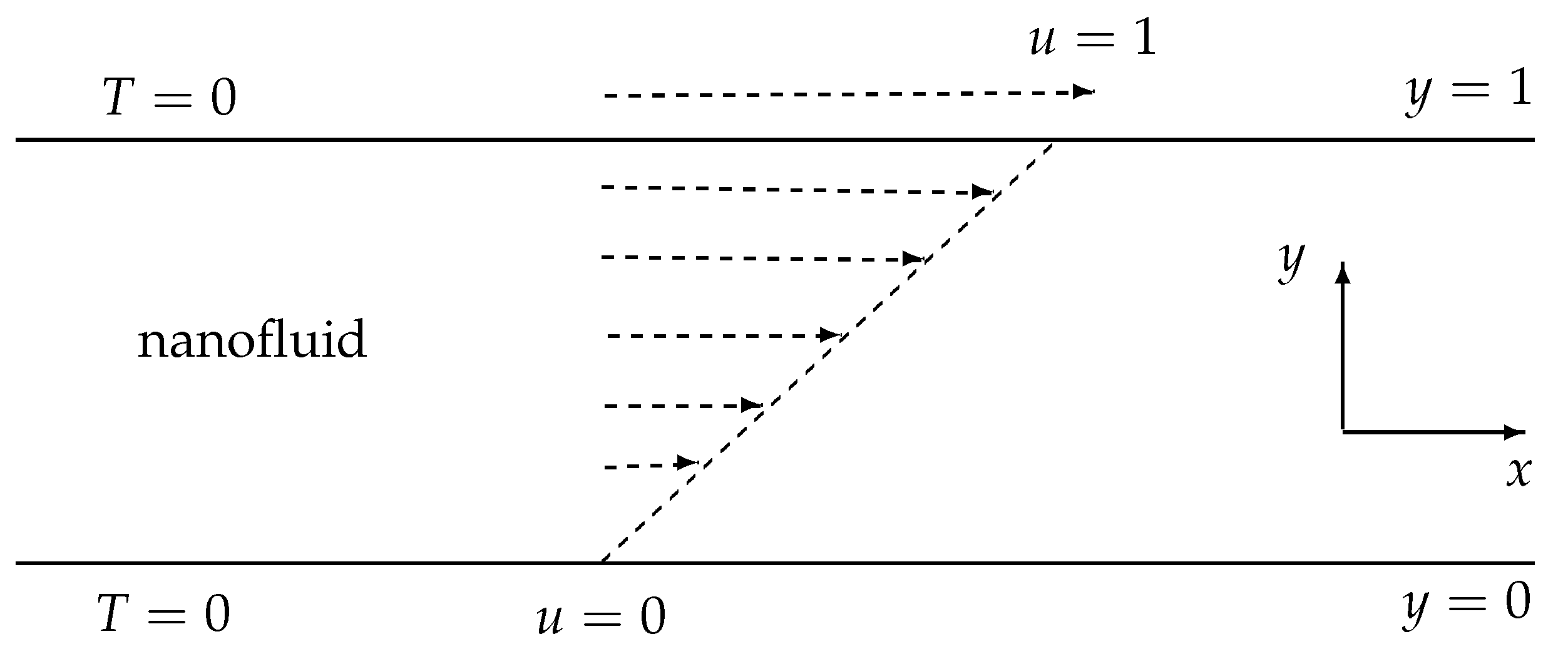
  • We assume the flow of a VFBN in a channel of infinite longitudinal extent. We therefore assume that the flow is fully developed in the x-direction and, hence, that flow quantities are independent of x.
    This allows us to focus our attention on the primary effects of shear banding on HTR and Therm-C enhancement without the complications of 2D (or indeed 3D) computations.
  • We assume that the shear banding is driven by constitutive instabilities via the Giesekus viscoelastic constitutive model.
    The exact mechanisms of shear banding, whether via constitutive instabilities or via flow inhomogeneities, are still areas of active research. Indeed, even for shear banding via constitutive instabilities, at least two viscoelastic constitutive models have been advanced. None of these considerations however detract from the primary aim to investigate the broader effects of shear banding on HTR and Therm-C enhancement.
  • We assume spherical nanoparticles that are homogeneously mixed with the base-fluid.
    The size, shape, distribution, orientation, etc., of the nanoparticles are still wide open areas with regard to investigating the optimal conditions for HTR and Therm-C enhancement. However, these considerations do not detract from the primary aim—to investigate the broader effects of nanoparticles on HTR and Therm-C enhancement.

2.2. Dimensionless Governing Equations

The development of the governing equations for the VFBN is adapted from [1]. Using the notation of [1], the relevant equations in dimensionless form are,
· u = 0 ,
Re n f D u D t = Re n f p + · σ ,
Pe n f D T D t = · κ n f T + Br Q D + δ 1 exp T 1 + α T ,
τ + ε τ 2 + De λ ¯ ( T ) τ τ D D t ln 1 + α T = η p ( T ) ( 1 ϕ ) 5 S ,
with,
Q D = γ S : τ + ( 1 γ ) η s ( T ) ( 1 ϕ ) 5 S : S ,
η s ( T ) = 1 β exp ( α T ) , ( η s ) n f = η s ( T ) ( 1 ϕ ) 5 ,
η p ( T ) = β e ( α T ) , ( η p ) n f = η p ( T ) ( 1 ϕ ) 5 ,
η = η s ( T ) + η p ( T ) , η n f = η ( 1 ϕ ) 5 ,
λ ¯ ( T ) = 1 1 + α T exp ( α T ) ,
κ n f = κ s + ( 1 χ ) κ f ( χ 1 ) ϕ ( κ f κ s ) κ s + ( 1 χ ) κ f + ϕ ( κ f κ s ) ( 1 + α A 2 T ) ,
where,
σ = τ + ( η s ) n f S , S = 1 2 u + ( u ) T .
The non-dimensional variables and dimensionless parameters used in Equations (1)–(11) are defined in the nomenclature at the end of the article. In particular, p is the pressure field; ε is the Giesekus non-linear parameter; σ is the total stress tensor; S is the rate of deformation tensor; τ is the polymer stress tensor; ( η s ) n f is the solvent viscosity for the nanofluid; ( η p ) n f is the polymer viscosity for the nanofluid; η n f is the total viscosity for the nanofluid; κ n f is the thermal conductivity for the nanofluid; α is the activation energy parameter; β is the polymer to total viscosity ratio; Br is the Brinkman number; δ 1 is the Frank-Kamenetskii parameter; De is the Deborah number; Pr is the Prandtl number; Pe is the Peclet number; Re is the Reynolds number, and the subscript ( ) n f represent nanofluid. Each os the nanofluid quantities, ( ) n f , is obtained as a linear combination of the contributions from the solid nanoparticles, ( ) s , and the base-fluid, ( ) f ;
( ) n f = ϕ ( ) s + ( 1 ϕ ) ( ) f .
The notations and D / D t represent the usual gradient and material-derivative operators respectively.

2.3. Initial and Boundary Conditions

The following initial and boundary conditions apply
u ( 0 , y ) = 0 , T ( 0 , y ) = 0 , τ ( 0 , y ) = 0 , for 0 y 1 ,
u ( t , 0 ) = 0 , u ( t , 1 ) = 1 , T ( t , 0 ) = 0 , T ( t , 1 ) = 0 , for t 0 .

3. Numerical and Computational Algorithms

The semi-implicit numerical scheme for the longitudinal velocity component is
Re n f u ( n + 1 ) u ( n ) Δ t = Re n f G + y τ 12 ( n ) + ( η s ) n f ( n ) 2 y 2 u ( n + ξ ) + y u ( n ) y ( η s ) n f ( n ) ,
where
u ( n + ξ ) = ξ u ( n + 1 ) + ( 1 ξ ) u ( n ) .
Therefore, the longitudinal velocity updates in time to u ( n + 1 ) , via
r 1 u j 1 ( n + 1 ) + ( Re n f + 2 r 1 ) u j ( n + 1 ) r 1 u j + 1 ( n + 1 ) = Re n f G + Re n f u j ( n ) + Δ t y τ 12 ( n ) + ( 1 ξ ) Δ t ( η s ) n f ( n ) 2 y 2 u ( n ) + ( 1 β ) Δ t y u ( n ) y ( η s ) n f ( n ) ,
where
r 1 = ξ ( η s ) n f ( n ) Δ t Δ y 2 .
A similar semi-implicit numerical scheme for the temperature is
Pe n f T t = κ n f ( n ) 2 y 2 T ( n + ξ ) + y T ( n ) y κ n f ( n ) + Br Q D ( n ) + δ 1 exp T ( n ) 1 + α T ( n ) .
leading to,
r 2 T j 1 ( n + 1 ) + ( Pe n f + 2 r 2 ) T j ( n + 1 ) r 2 T j + 1 ( n + 1 ) = Pe n f T j ( n ) + ( 1 ξ ) Δ t κ n f 2 y 2 T ( n ) + Δ t y T ( n ) y κ n f ( n ) + 2 ( 1 γ ) Δ t Br ( η s ) n f ( n ) y u ( n ) 2 + 2 Δ t Br γ τ 12 ( n ) y u ( n ) ,
where
r 2 = ξ κ n f Δ t Δ y 2 .
Finally, the semi-implicit numerical scheme for the polymeric-stress is
τ ( n + ξ ) + ε ( τ 2 ) ( n ) + De λ ¯ ( n ) τ ( n + 1 ) τ ( n ) Δ t = explicit terms .
This leads to the direct solution
( De λ ¯ ( n ) + ξ Δ t ) τ ( n + 1 ) = explicit terms .
where the respective explicit terms are
[ De λ ¯ ( n ) ( 1 ξ ) Δ t ] τ 11 ( n ) + Δ t De λ ¯ ( n ) τ 12 ( n ) y u ( n ) + τ 11 ( n ) y log 1 + α T ( n )
ε Δ t ( τ 11 2 + τ 12 2 ) , [ De λ ¯ ( n ) ( 1 ξ ) Δ t ] τ 12 ( n ) + Δ t De λ ¯ ( n ) τ 22 ( n ) y u ( n ) + τ 12 ( n ) y log 1 + α T ( n )
+ Δ t ( η p ) n f y u ( n ) ε Δ t ( τ 11 τ 12 + τ 12 τ 22 ) ,
[ De λ ¯ ( n ) ( 1 ξ ) Δ t ] τ 22 ( n ) + Δ t De λ ¯ ( n ) τ 22 ( n ) y log 1 + α T ( n ) ε Δ t ( τ 12 2 + τ 22 2 ) .

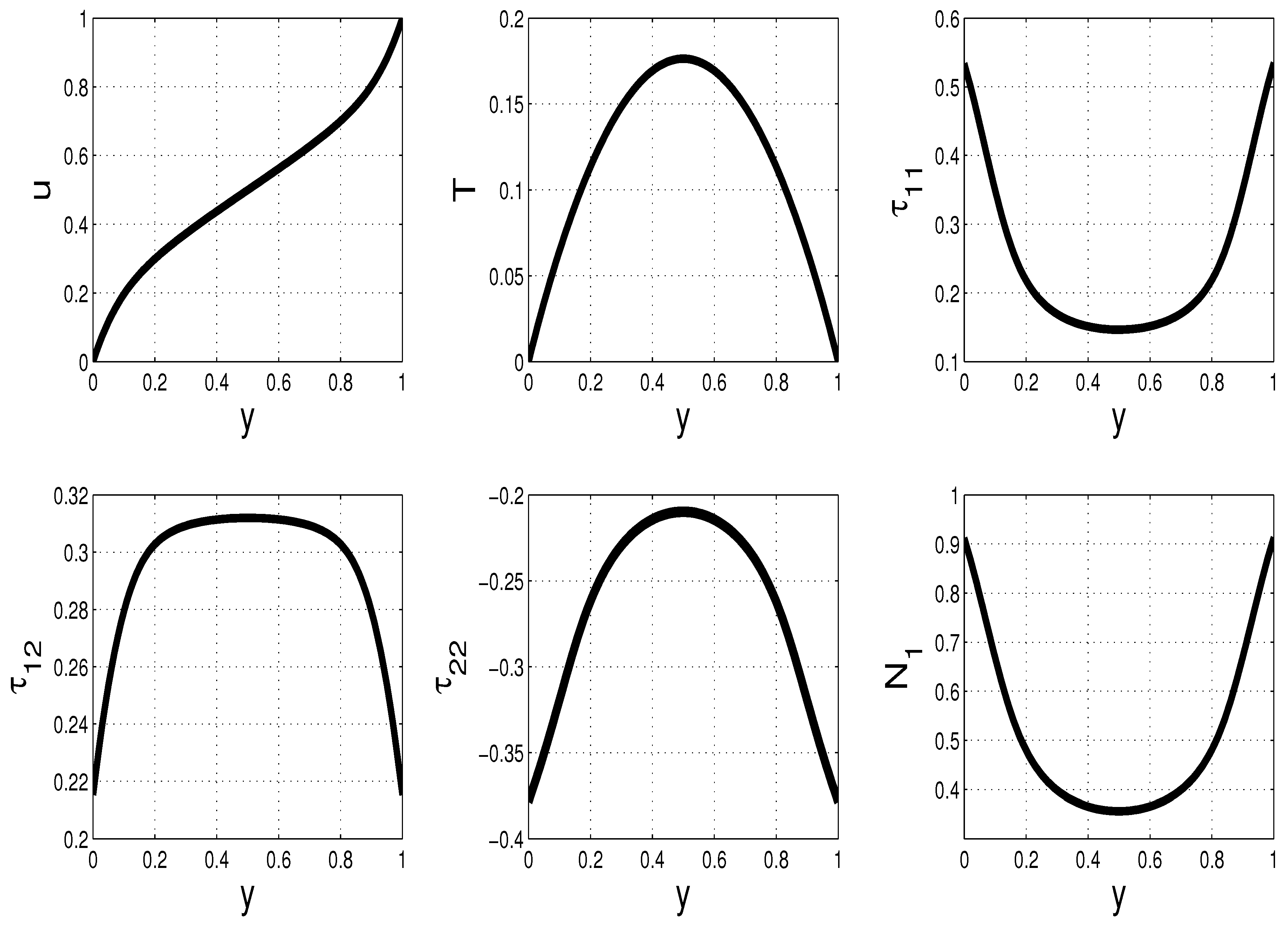
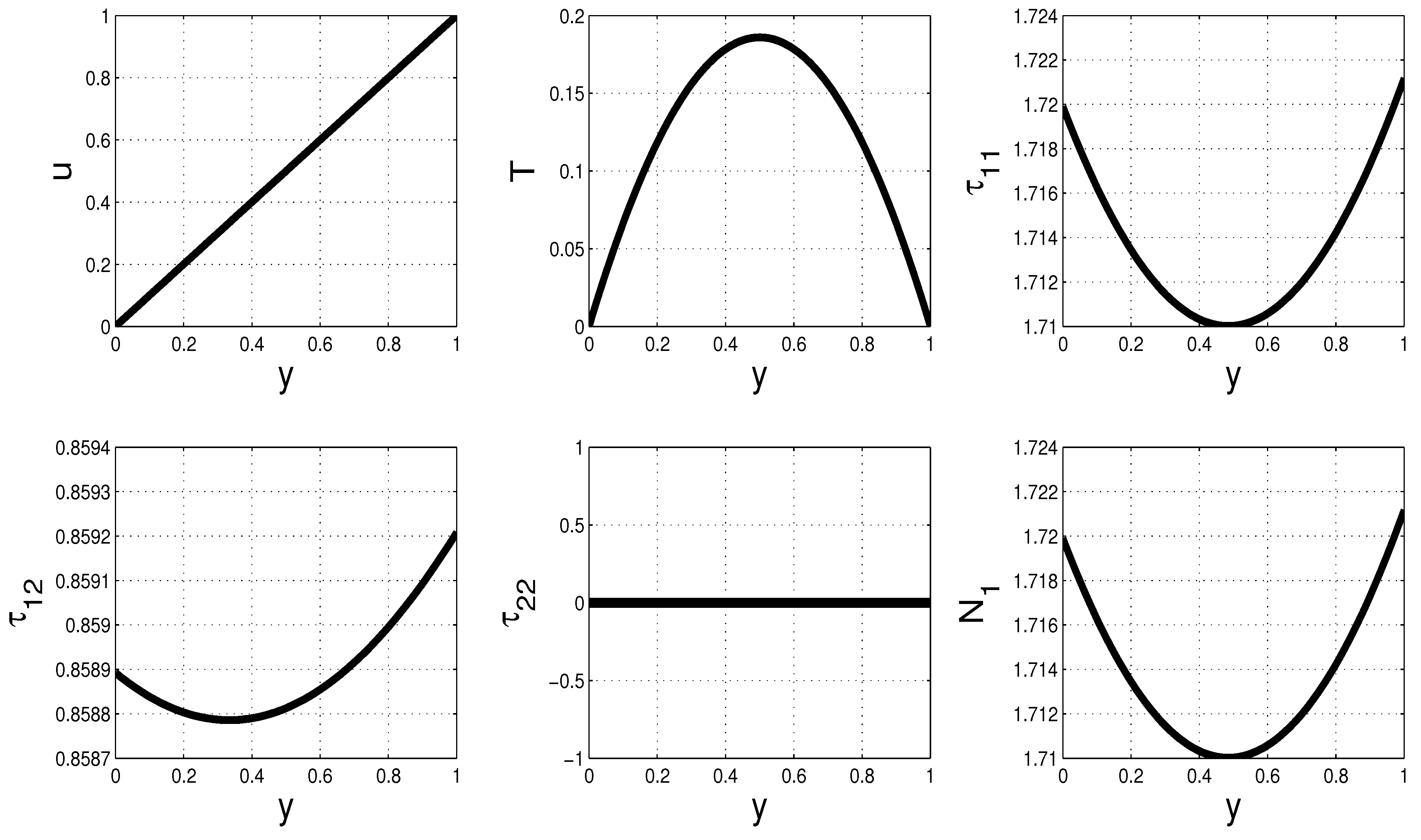
3.1. Graphical and Qualitative Results

Unless otherwise indicated, the following list of default values will be assumed for the various quantities and parameters:
α = 0.01 , Br = 1 , Re = 1 , Pr = 1 , De = 2 , γ = 0.5 , β = 0.2 , Δ y = 0.01 , Δ t = 0.01 , t = 50 , δ 1 = 0.5 , ζ = 1 , ϕ = 0.04 , ε = 0.5 , A 2 = 0.2 , χ = 3 , ξ = 1 .

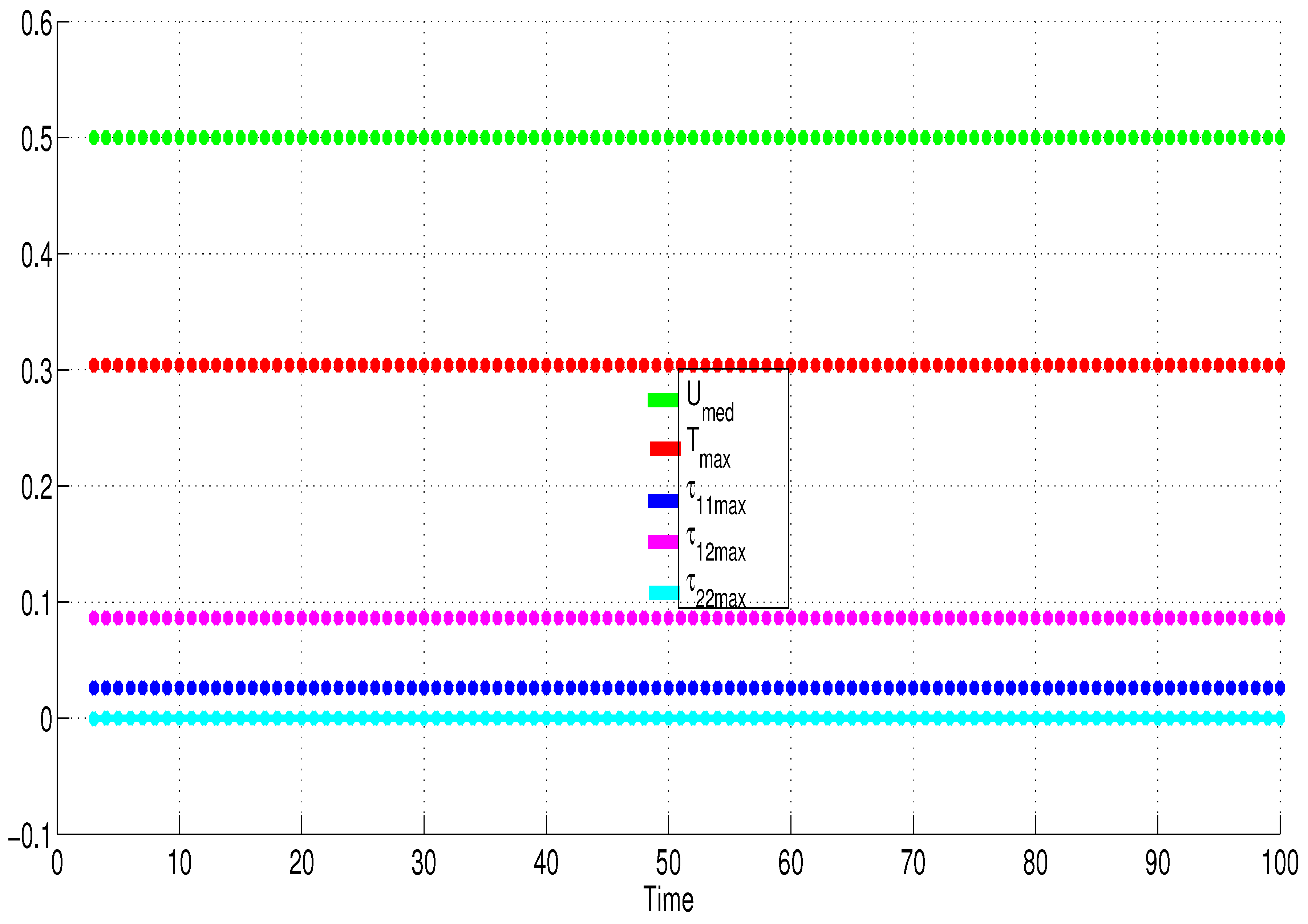
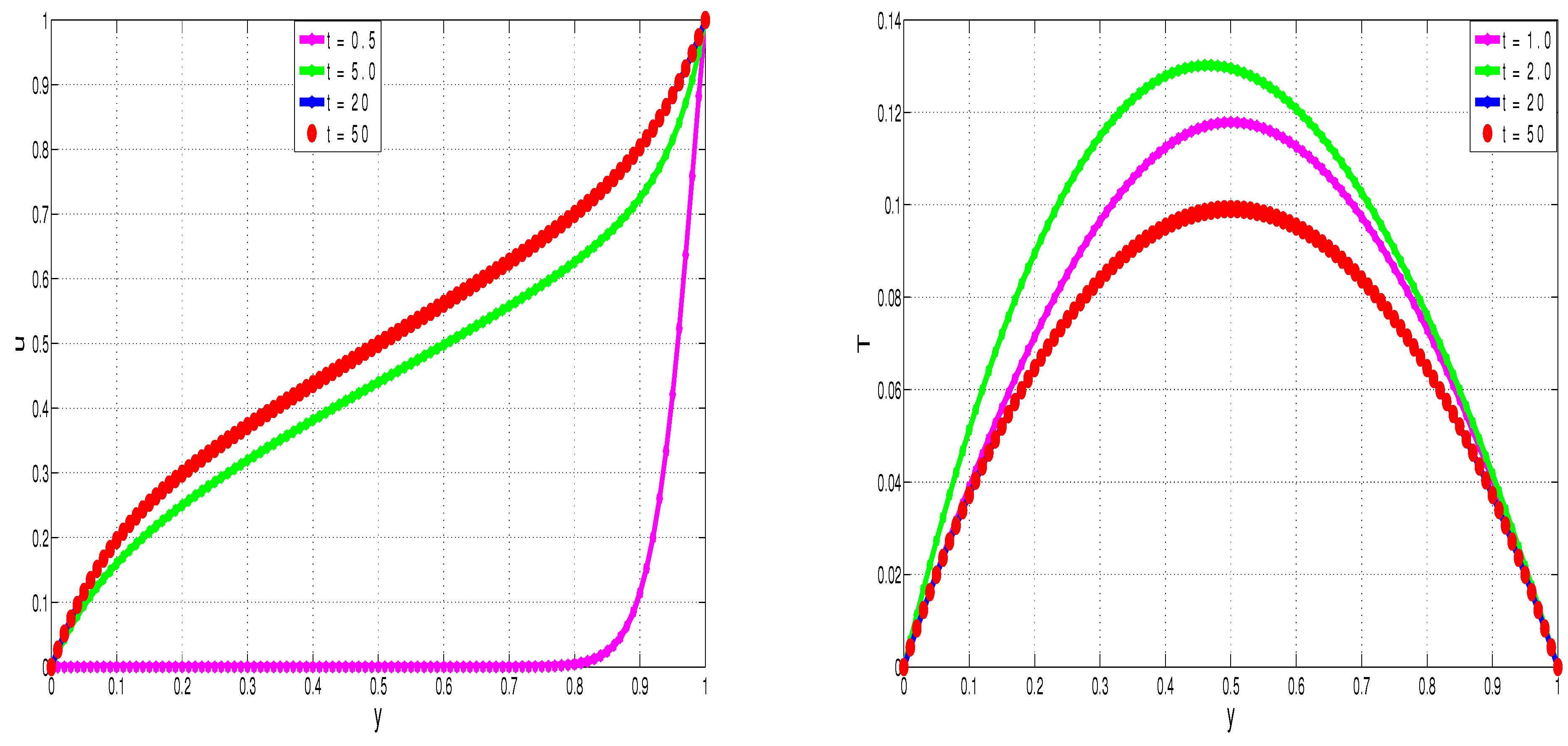
3.2. Time Development of Steady Smooth Solutions

Figure 2, Figure 3, Figure 4 and Figure 5 show the development (in time) of flow quantities until steady states are reached. Specifically, Figure 2 illustrates the transient development of nanofluid velocity, u, and nanofluid temperature, T. The fluid flow is driven by shear forces acting longitudinally on the upper wall. Initially, the bulk fluid is at rest. We notice from Figure 2—as expected—that the fluid velocity develops steadily in time from the initial state until the linear shear flow profile is achieved. Similarly, the fluid temperature is initially at zero throughout the flow geometry. As the flow develops in time, the exothermic reactions and mechanical dissipation processes taking place in the bulk flow lead to inevitable temperature increases in the bulk fluid. The channel walls are otherwise maintained at isothermal temperatures. We therefore notice from Figure 2—as expected—that the bulk flow temperature gradually increases in time until steady state parabolic temperature profiles are reached.
Figure 3 and Figure 4 show the time development of polymer stresses, τ 11 , τ 22 , τ 12 , and, hence, also of the second normal stress difference N 1 = τ 11 τ 22 . As with the velocity and temperature profiles, we notice that the polymer stresses converge to fixed (reproducible) steady state solutions. The fixed (reproducibility) nature of the converged steady solutions is specifically illustrated in Figure 5, where the same converged values are obtained irrespective of the subsequent time of additional computation. For example, once the solutions converge to steady-state, at say, time t = 20 , then extending the computations to say, time t = 100 , will not change (qualitatively and quantitatively) the steady solutions.

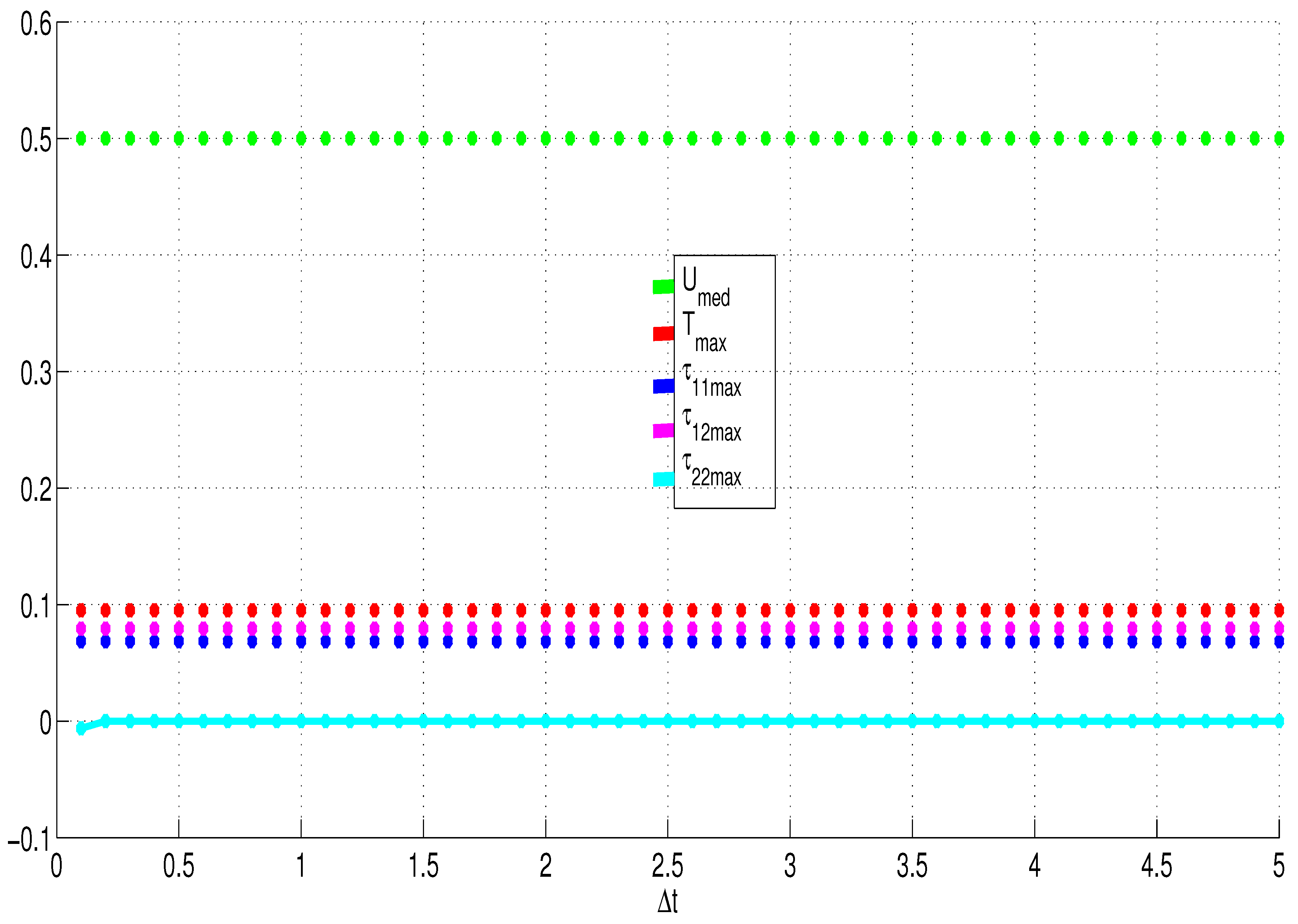
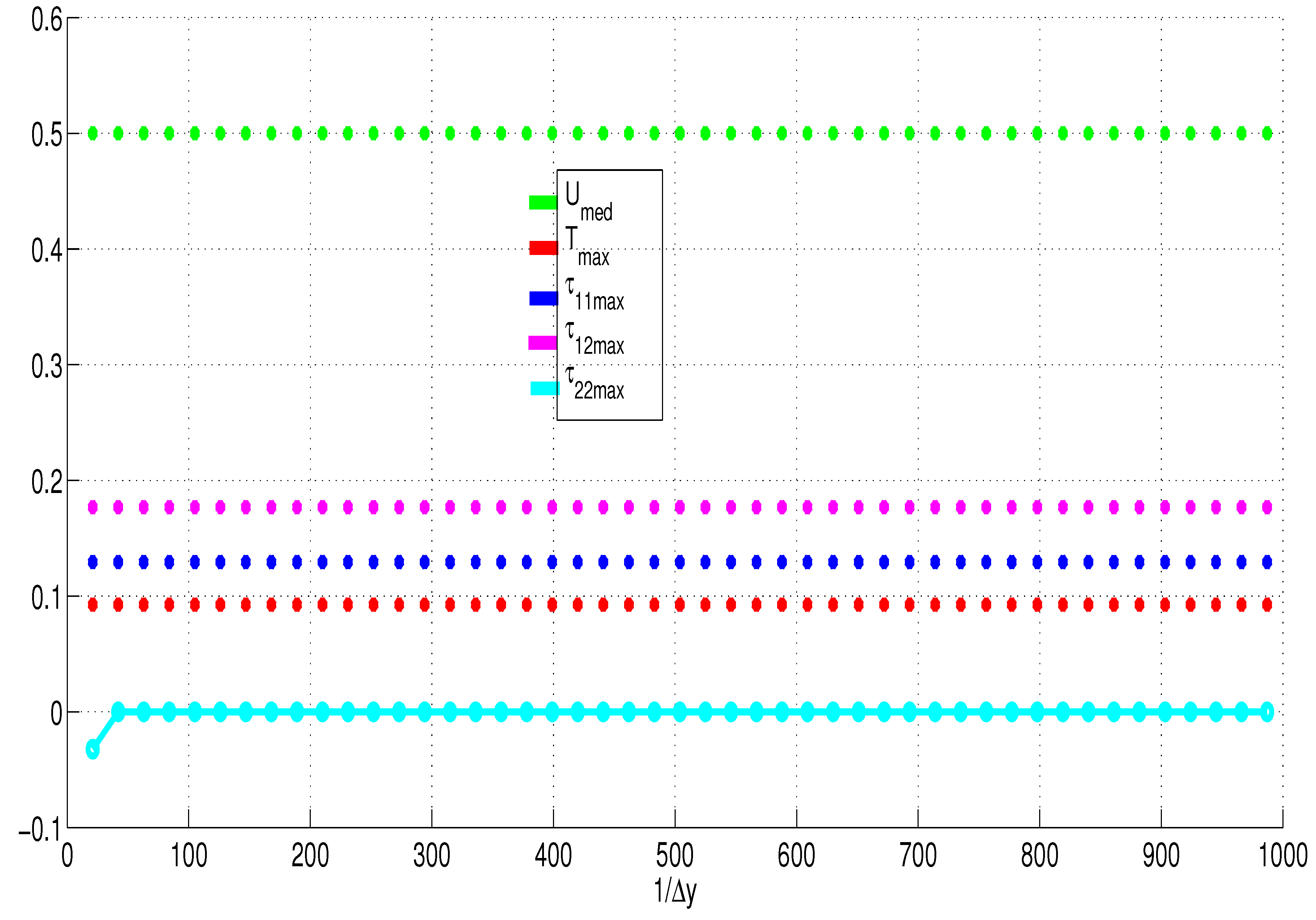
3.3. Mesh-Size and Time-Step and Convergence

Our numerical algorithms use central differences to approximate the space derivatives. This means that our numerical schemes are second-order accurate in space. The accuracy in time is determined by the choice of ξ . Our computational results are all obtained with ξ = 1 . This means that our numerical algorithms (with ξ = 1 ) are essentially first-order accurate in time. Taking, for example, ξ = 0.5 , as in the Crank–Nicolson scheme, would increase the accuracy in time to second-order. The choice ξ = 0.5 would however require small time-steps ( Δ t 1 ) to ensure that the computations converge in time. For this reason, we employ ξ = 1 ; hence, we are free to use large time-steps, as illustrated in Figure 6. As shown in Figure 7, our numerical and computational algorithms also converge even with moderate values of the mesh-size, Δ y 1 .
Figure 6 and Figure 7 therefore demonstrate—as required—that our numerical algorithms are largely independent of both mesh-size and time-step. Specifically, the computational algorithms efficiently reproduce the expected solutions for a broad range of mesh sizes and time-steps.

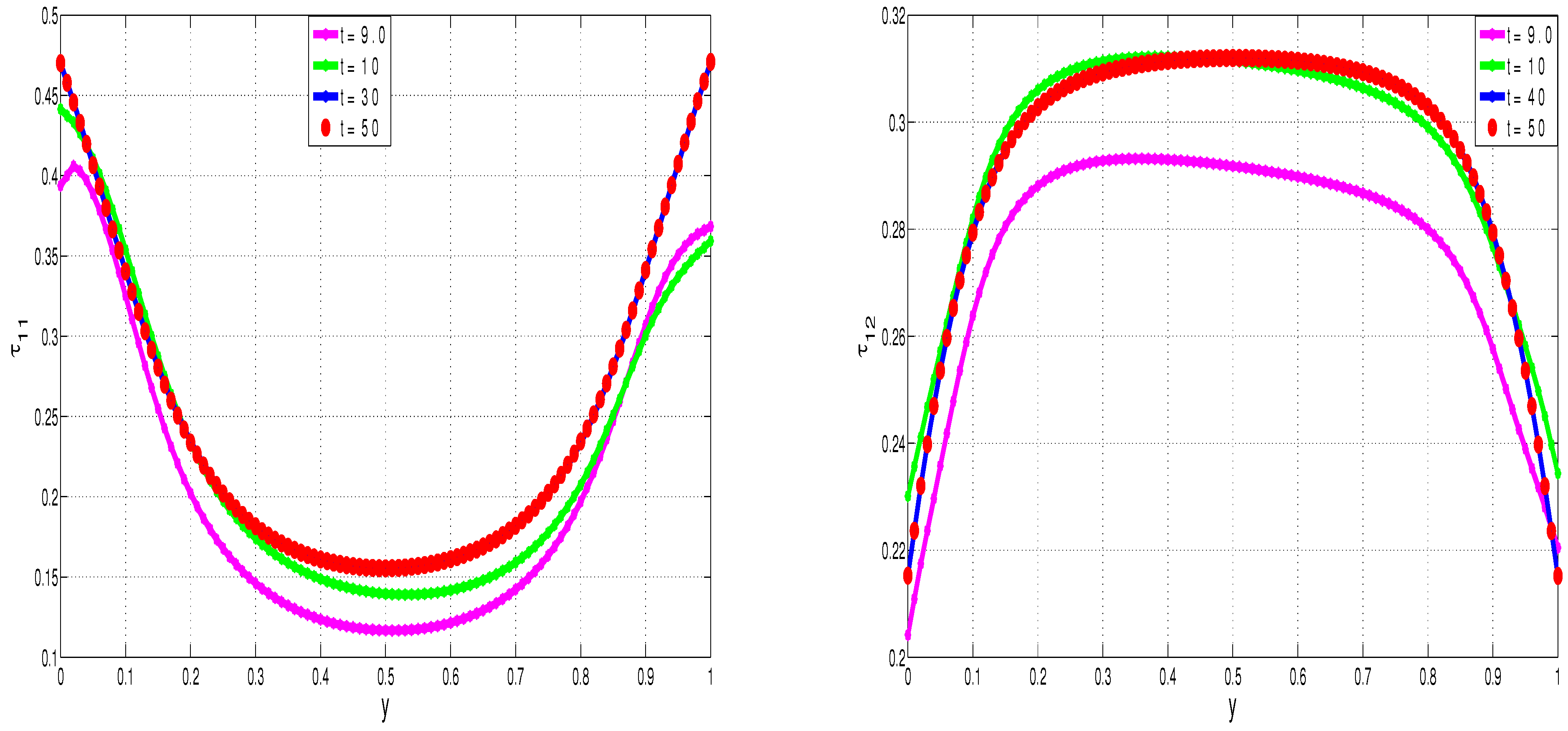
3.4. Development of Shear Banding

As noted in the introduction, shear banding phenomena in the shear flow of viscoelastic fluids represent observable and physical discontinuities in the shear rate profiles of the flow velocity. Shear banding phenomena have been observed in the shear flow of polymeric fluids of various types, including, for example, worm-like micelle solutions, polymer solutions, foams, telechelic polymers, granular flows, soft glasses, and polymer melts.
As noted in the introduction, there are two main scientifically-agreed mechanisms for shear banding, namely flow-induced inhomogeneities and constitutive instabilities. The Rolie-Poly viscoelastic constitutive model has been developed to explain the shear banding phenomena via flow-induced inhomogeneities. The Johnson-Segalman and Giesekus viscoelastic constitutive models allow for the mechanisms of the shear banding phenomena via constitutive instabilities if certain values of the viscoelastic material parameters are taken.
Specifically, when β = 0.95 and ε = 2 in the Giesekus constitutive model, we note that the steady solutions (for the velocity u, temperature T, polymer-stresses τ 11 , τ 12 , τ 22 , and first normal stress difference N 1 ) exhibit shear banding phenomena, see Figure 8.
As indicated, and as in [27], the shear banding phenomena depicted in Figure 8 is linked to the viscoelastic parameters, specifically the polymer-to-total viscosity ratio ( β ) and the Giesekus nonlinear parameter ( ε ) in the present study. In [27], the shear banding was linked to β and the Johnson-Segalman parameter. Taking ε = 0 reduces the Giesekus viscoelastic constitutive model to the Oldroyd-B model, which is not capable of exhibiting shear banding, as illustrated in Figure 9 for the velocity u, temperature T, polymer-stresses τ 11 , τ 12 , τ 22 , and first normal stress difference N 1 . Similarly, varying the values of β shows that the onset and prevalence of shear banding is linked to higher values of β , as long as the value of ε is high enough, see Figure 10.
The phenomena of shear banding via constitutive instabilities is extensively investigated in [27] using the Johnson-Segalman viscoelastic constitutive model. In particular, it is conclusively demonstrated in [27] that shear banded solutions are essentially weak solutions of the governing partial differential equations for viscoelastic fluid flow and that an infinite number of such solutions exist for any set of shear banding material parameters. However, the results in [27] illustrate that, for each set of shear banding material parameter values, the computational results will always reproduce the same unique (albeit weak) solution! The unique selected shear rate path has been scientifically explained using the concept of stress diffusion as demonstrated in [28].
Figure 11 and Figure 12 illustrate the transient development of steady shear banded solutions, demonstrating, as in [27,28] the robustness and reproducibility of the shear banded solutions.

3.5. Thermal Runway

In industrial applications involving exothermic reactions, it is fundamental to ensure thermal stability and avoid thermal runaway phenomena. Thermal runaway can be demonstrated by increasing the values of the exothermic reaction parameter, δ 1 . Figure 13 illustrates the effects of δ 1 on the steady-state VFBN velocity and temperature, specifically the drastic increase of temperature with increasing δ 1 .
Figure 14 gives a comparative illustration of the thermal runaway phenomena for Newtonian fluid-based and viscoelastic fluid-based nanofluids, i.e., NFBN and VFBN. The results for the Giesekus type VFBN computations are consistent with those in [23], which are based on the particle-free Oldroyd-B fluid computations. In particular, our results demonstrate that NFBN are more susceptible to thermal runaway than are the VFBN. This is consistent with the results in [23]. Essentially, the current results and those in [23] demonstrate that fluid viscoelasticity fundamentally acts to reduce large temperature build-ups in the exothermic shear flow setup and, hence, can be used to mitigate against rapid and finite-time temperature blow-up, i.e., thermal runaway. The present study will additionally demonstrate that shear banding phenomena can further enhance these favorable HTR characteristics of viscoelastic fluids, thus extending the scope of the investigations in [1,23].

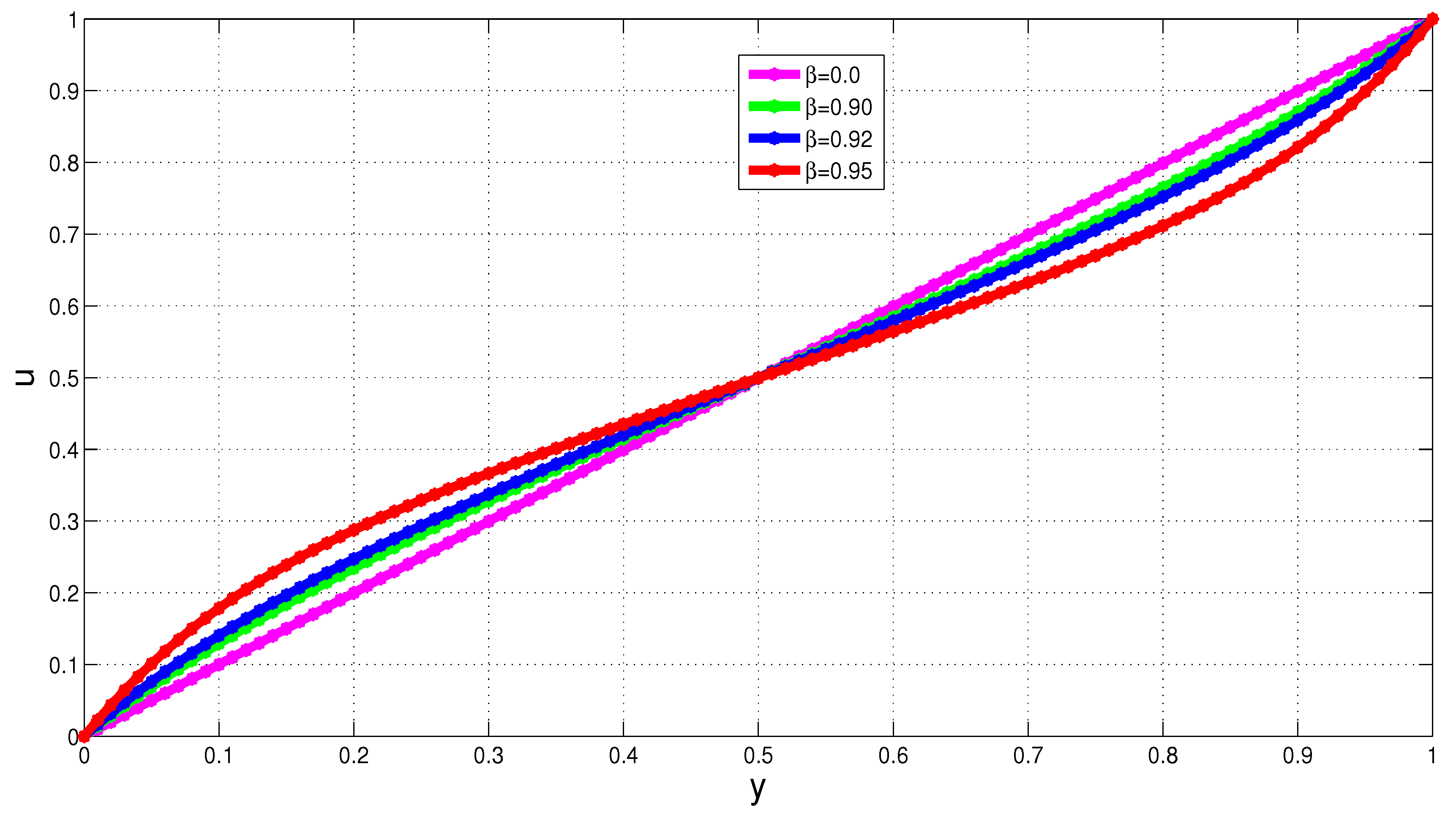
4. Parameter Dependence of Solutions under Shear Banding Conditions

The dependence of thermal runaway on δ 1 and that of shear banding on β and ε have already been illustrated.
We now demonstrate, more generally, the sensitivity of the flow variables (solutions) to variations in these and other embedded parameters under shear banding conditions, i.e., β = 0.95 , ε = 2 .
Figure 15 shows the dependence of the VFBN temperature field and thermal conductivity on nanoparticle volume fraction, ϕ . As expected, both the VFBN temperature and thermal conductivity increase with increasing ϕ . This is clearly expected, since the higher the concentration of heat-conducting nanoparticles (i.e., higher ϕ ), the higher the corresponding Therm-C capabilities of the resultant nanofluid, and hence, the higher the temperatures in the nanofluid.
Figure 16 shows the dependence of the VFBN velocity and temperature on the Brinkman number, Br. Being directly proportional to the heat sources in the energy equation, increases in the Brinkman number, Br, would correspondingly increase the fluid temperature. Figure 16 also illustrates that the Brinkman number would not affect the shear banded nature of the velocity profile.
As with the thermal runaway analysis presented earlier (see Figure 13 and Figure 14) as well as the comparative literature, say [23,27], Figure 17 shows, as expected, that VFBNs are more resistant to temperature increases than NFBN.
Figure 17 additionally shows, as already expected, that the nanofluid temperature increases with increasing Br, but it decreases with increasing polymer viscosity, β . This further illustrates the viability of viscoelasticity (for which the polymer viscosity is a proxy) in dampening unwanted temperature increases and temperature blow-ups. As in [23], Figure 17 shows that the increase of temperature, with respect to Br, is linear for viscoelastic flow as opposed to the exponential increase observed with respect to δ 1 . This therefore means that increases in Br are not expected to lead to thermal runaway in shear flow of VFBN.
We conclude by demonstrating the expected increase of both the VFBN temperature and thermal conductivity with increasing activation energy parameter, α , see Figure 18. As would be logically expected, the higher the activation energy strength, the faster the exothermic reaction processes and, hence, the higher the nanofluid thermal conductivities and obtainable temperatures, as illustrated in Figure 18.

5. Concluding Remarks

We employed a versatile and convergent numerical and computational algorithm, based on semi-implicit finite-difference methods to study the shear banding and thermal runaway characteristics of VFBN, which use Giesekus base fluids. We observed remarkable HTR and Therm-C enhancement in the VFBN under shear banding conditions of the material parameters. Specifically, we demonstrated that the VFBN are less susceptible to the thermal runaway than NFBN, and that this reduced susceptibility to thermal runaway phenomena is further enhanced under shear banding conditions—in particular, under increased polymer viscosity conditions.

Author Contributions

Conceptualization, T.C.; methodology, T.C.; software, T.C. and I.K.; validation, T.C. and I.K.; formal analysis, T.C. and I.K.; investigation, T.C. and I.K.; resources, T.C., I.K. and A.G.; data curation, T.C. and I.K.; writing—original draft preparation, I.K.; writing—review and editing, T.C., I.K. and A.G.; visualization, T.C., I.K. and A.G.; supervision, T.C. and A.G.; project administration, T.C., I.K. and A.G.; funding acquisition, T.C. All authors have read and agreed to the published version of the manuscript.

Funding

This research received no external funding.

Institutional Review Board Statement

Not applicable.

Informed Consent Statement

Not applicable.

Data Availability Statement

Not applicable.

Conflicts of Interest

The authors declare no conflict of interest.

Nomenclature

The following nomenclature are used in this manuscript:
Variables
ε Giesekus non-linear parameter
( η s ) n f Solvent viscosity for the VFBN
( η p ) n f polymer viscosity for the VFBN
η n f total viscosity for the VFBN
κ n f thermal conductivity for the VFBN
G ^ non-isothermal viscoelastic parameter
ppressure field
S rate of deformation tensor
σ total stress tensor
tTime
TTemperature field
τ polymer stress tensor
u = ( u , v ) velocity field
x = ( x , y ) 2D Cartesian space coordinates
Parameters
α activation energy parameter
β polymer to total viscosity ratio
BrBrinkman number
δ 1 Frank–Kamenetskii parameter
DeDeborah number
PrPrandtl number
PePeclet number
ReReynolds number
Abbreviations  
VFBNviscoelastic fluid-based nanofluid
NFBNNewtonian fluid-based nanofluid
HTRheat transfer rate
Therm-Cthermal conductivity

References

  1. Khan, I.; Chinyoka, T.; Gill, A. Computational analysis of the dynamics of generalized-viscoelastic-fluid-based nanofluids subject to exothermic reaction in shear flow. J. Nanofluids 2022, 11. in press. [Google Scholar]
  2. Sheikhpour, M.; Arabi, M.; Kasaeian, A.; Rabei, A.R.; Taherian, Z. Role of Nanofluids in Drug Delivery and Biomedical Technology: Methods and Applications. Nanotechnol. Sci. Appl. 2020, 13, 47–59. [Google Scholar] [CrossRef] [PubMed]
  3. Wong, K.V.; Leon, O.D. Applications of Nanofluids: Current and Future. In Nanotechnology and Energy; Jenny Stanford Publishing: Dubai, United Arab Emirates, 2017; pp. 105–132. [Google Scholar] [CrossRef]
  4. Li, F.C.; Yang, J.C.; Zhou, W.W.; He, Y.R.; Huang, Y.M.; Jiang, B.C. Experimental study on the characteristics of thermal conductivity and shear viscosity of viscoelastic-fluid-based nanofluids containing multiwalled carbon nanotubes. Thermochim. Acta 2013, 556, 47–53. [Google Scholar] [CrossRef]
  5. Sundar, L.S.; Naik, M.T.; Sharma, K.V.; Singh, M.K.; Reddy, T.C.S. Experimental investigation of forced convection heat transfer and friction factor in a tube with Fe3O4 magnetic nanofluid. Exp. Therm. Fluid Sci. 2012, 37, 65–71. [Google Scholar] [CrossRef]
  6. Yang, J.C.; Li, F.C.; Zhou, W.W.; He, Y.R.; Jiang, B.C. Experimental investigation on the thermal conductivity and shear viscosity of viscoelastic-fluid-based nanofluids. Int. J. Heat Mass Transf. 2012, 55, 3160–3166. [Google Scholar] [CrossRef]
  7. Sajadi, A.R.; Kazemi, M.H. Investigation of turbulent convective heat transfer and pressure drop of TiO2/water nanofluid in circular tube. Int. Commun. Heat Mass Transf. 2011, 38, 1474–1478. [Google Scholar] [CrossRef]
  8. Kleinstreuer, C.; Feng, Y. Experimental and theoretical studies of nanofluid thermal conductivity enhancement: A review. Nanoscale Res. Lett. 2011, 6, 1–13. [Google Scholar]
  9. Kalteh, M.; Abbassi, A.; Saffar-Avval, M.; Harting, J. Eulerian–Eulerian two-phase numerical simulation of nanofluid laminar forced convection in a microchannel. Int. J. Heat Fluid Flow 2011, 32, 107–116. [Google Scholar] [CrossRef]
  10. Kondaraju, S.; Jin, E.K.; Lee, J.S. Investigation of heat transfer in turbulent nanofluids using direct numerical simulations. Phys. Rev. E 2010, 81, 016304. [Google Scholar] [CrossRef]
  11. Özerinç, S.; Kakaxcx, S.; Yazıcıoǧlu, A.G. Enhanced thermal conductivity of nanofluids: A state-of-the-art review. Microfluid. Nanofluidics 2010, 8, 145–170. [Google Scholar] [CrossRef]
  12. VTerekhov, I.; Kalinina, S.V.; Lemanov, V.V. The mechanism of heat transfer in nanofluids: State of the art (review), Part 1, Synthesis and properties of nanofluids. Thermophys. Aeromech. 2010, 17, 1–14. [Google Scholar] [CrossRef]
  13. Chandrasekar, M.; Suresh, S. Determination of Heat Transport Mechanism in Aqueous Nanofluids Using Regime Diagram. Chin. Phys. Lett. 2009, 26, 124401. [Google Scholar] [CrossRef]
  14. Behzadmehr, A.; Saffar-Avval, M.; Galanis, N. Prediction of turbulent forced convection of a nanofluid in a tube with uniform heat flux using a two phase approach. Int. J. Heat Fluid Flow 2007, 28, 211–219. [Google Scholar] [CrossRef]
  15. Xiao-Feng, Z.; Lei, G. Effect of multipolar interaction on the effective thermal conductivity of nanofluids. Chin. Phys. 2007, 16, 2028. [Google Scholar] [CrossRef]
  16. Maiga, S.E.B.; Palm, S.J.; Nguyen, C.T.; Roy, G.; Galanis, N. Heat transfer enhancement by using nanofluids in forced convection flows. Int. J. Heat Fluid Flow 2005, 26, 530–546. [Google Scholar] [CrossRef]
  17. Roy, G.; Nguyen, C.T.; Lajoie, P.R. Numerical investigation of laminar flow and heat transfer in a radial flow cooling system with the use of nanofluids. Superlattices Microstruct. 2004, 35, 497–511. [Google Scholar] [CrossRef]
  18. Xuan, Y.; Li, Q. Investigation on convective heat transfer and flow features of nanofluids. Heat Transf. 2003, 125, 151–155. [Google Scholar] [CrossRef] [Green Version]
  19. Keblinski, P.; Phillpot, S.R.; Choi, S.U.; Eastman, J.A. Mechanisms of heat flow in suspensions of nano-sized particles (nanofluids). Int. J. Heat Mass Transf. 2002, 45, 855–863. [Google Scholar] [CrossRef]
  20. Eastman, J.A.; Choi, S.U.; Li, S.; Yu, W.; Thompson, L.J. Anomalously increased effective thermal conductivities of ethylene glycol-based nanofluids containing copper nanoparticles. Appl. Phys. Lett. 2001, 78, 718–720. [Google Scholar] [CrossRef]
  21. Xuan, Y.; Li, Q. Heat transfer enhancement of nanofluids. Int. J. Heat Fluid Flow 2000, 21, 58–64. [Google Scholar] [CrossRef]
  22. Li, S.; Eastman, J.A. Measuring thermal conductivity of fluids containing oxide nanoparticles. J. Heat Transf. 1999, 121, 280–289. [Google Scholar]
  23. Chinyoka, T. Comparative Response of Newtonian and Non-Newtonian Fluids Subjected to Exothermic Reactions in Shear Flow. Int. J. Appl. Comput. Math. 2021, 7, 1–19. [Google Scholar] [CrossRef]
  24. Abuga, J.G.; Chinyoka, T. Benchmark solutions of the stabilized computations of flows of fluids governed by the Rolie-Poly constitutive model. J. Phys. Commun. 2020, 4, 015024. [Google Scholar] [CrossRef]
  25. Abuga, J.G.; Chinyoka, T. Numerical Study of Shear Banding in Flows of Fluids Governed by the Rolie-Poly Two-Fluid Model via Stabilized Finite Volume Methods, Journal of Physics Communications. Processes 2020, 8, 810. [Google Scholar] [CrossRef]
  26. Ireka, I.E.; Chinyoka, T. Analysis of shear banding phenomena in non-isothermal flow of fluids governed by the diffusive Johnson–Segalman model. Appl. Math. Model. 2016, 40, 3843–3859. [Google Scholar] [CrossRef]
  27. Chinyoka, T. Suction-Injection Control of Shear Banding in Non-Isothermal and Exothermic Channel Flow of Johnson–Segalman Liquids. ASME J. Fluids Eng. 2011, 133, 071205. [Google Scholar] [CrossRef]
  28. Ireka, I.E.; Chinyoka, T. Non-isothermal flow of a Johnson–Segalman liquid in a lubricated pipe with wall slip. J. Non-Newton. Fluid Mech. 2013, 192, 20–28. [Google Scholar] [CrossRef]
  29. Chinyoka, T.; Goqo, S.P.; Olajuwon, B.I. Computational analysis of gravity driven flow of a variable viscosity viscoelastic fluid down an inclined plane. Comput. Fluids 2013, 84, 315–326. [Google Scholar] [CrossRef]
  30. Chinyoka, T. Poiseuille flow of reactive phan-thien-tanner liquids in 1D channel flow. J. Heat Transf. 2010, 132, 111701. [Google Scholar] [CrossRef]
  31. Chinyoka, T. Viscoelastic effects in double pipe single pass counterflow heat exchangers. Int. J. Numer. Methods Fluids 2009, 59, 677–690. [Google Scholar] [CrossRef]
  32. Chinyoka, T. Modeling of cross-flow heat exchangers with viscoelastic fluids. Nonlinear Anal. Real World Appl. 2009, 10, 3353–3359. [Google Scholar] [CrossRef]
  33. Chinyoka, T. Computational dynamics of a thermally decomposable viscoelastic lubricant under shear. J. Fluids Eng. 2008, 130, 121201. [Google Scholar] [CrossRef]
  34. Chinyoka, T. Numerical Simulation of Stratified Flows and Droplet Deformation in 2D Shear Flow of Newtonian and Viscoelastic Fluids. Ph.D. Thesis, Virginia Polytechnic Institute and State University (Virgina Tech), Blacksburg, VA, USA, 2004. [Google Scholar]
  35. Garci, J.P.; Manero, O.; Bautista, F.; Puig, J.E. Inhomogeneous flows and Shear banding formation in micellar solutions: Predictions of the BMP model. J. Non-Newton. Fluid Mech. 2012, 179, 43–54. [Google Scholar]
  36. Kim, Y.; Adams, A.; Hartt, W.H.; Larson, R.G.; Solomon, M.J. Transient, Near-wall shear-band dynamics in channel flow of wormlike micelle solutions. J. Non-Newton. Fluid Mech. 2016, 232, 77–87. [Google Scholar] [CrossRef] [Green Version]
  37. Hilliou, L.; Vlassopoulos, D. Time-periodic structures and instabilities in shear-thickening polymer solutions. Ind. Eng. Chem. Res. 2002, 41, 6246–6255. [Google Scholar] [CrossRef]
  38. Kabla, A.; Debrégeas, G. Local stress relaxation and shear banding in a dry foam under shear. Phys. Rev. Lett. 2003, 90, 258303. [Google Scholar] [CrossRef] [Green Version]
  39. Billen, J.; Wilson, M.; Baljon, A.R. Shear banding in simulated telechelic polymers. Chem. Phys. 2015, 446, 7–12. [Google Scholar] [CrossRef]
  40. Mueth, D.M.; Debregeas, G.F.; Karczmar, G.S.; Eng, P.J.; Nagel, S.R.; Jaeger, H.M. Signatures of granular microstructure in dense shear flows. Nature 2000, 406, 385–389. [Google Scholar] [CrossRef] [Green Version]
  41. Holmes, W.M.; Callaghan, P.T.; Vlassopoulos, D.; Roovers, J. Shear banding phenomena in ultrasoft colloidal glasses. J. Rheol. 2004, 48, 1085–1102. [Google Scholar] [CrossRef]
  42. Fang, Y.; Wang, G.; Tian, N.; Wang, X.; Zhu, X.; Lin, P.; Li, L. Shear inhomogeneity in poly (ethylene oxide) melts. J. Rheol. 2011, 55, 939–949. [Google Scholar] [CrossRef]
Figure 1. Geometry of the model problem.
Energies 15 01719 g001
Figure 2. Development of steady velocity profiles (left) and temperature profiles (right).
Energies 15 01719 g002
Figure 3. Development of steady polymer stress profiles; τ 11 -stress (left) and τ 22 -stress (right).
Energies 15 01719 g003
Figure 4. Development of steady τ 12 -stress profiles (left) and second normal stress difference ( N 1 ) profiles (right).
Energies 15 01719 g004
Figure 5. Development of steady maximum flow profiles.
Energies 15 01719 g005
Figure 6. Dependence of solutions on time-step size.
Energies 15 01719 g006
Figure 7. Dependence of solutions on mesh-size.
Energies 15 01719 g007
Figure 8. Development of shear bands for the Giesekus model with β = 0.95 , ε = 2 . The figures represent: Top-row from left to right velocity (u), temperature (T), and τ 11 -stress. Bottom-row from left to right τ 12 -stress, τ 22 -stress, and first normal stress difference ( N 1 ).
Energies 15 01719 g008
Figure 9. Absence of shear bands for the Oldroyd-B model with β = 0.95 , ε = 0 . Top-row from left to right velocity (u), temperature (T), and τ 11 -stress. Bottom-row from left to right τ 12 -stress, τ 22 -stress, and first normal stress difference ( N 1 ).
Energies 15 01719 g009
Figure 10. Development of shear banding with increasing β , where ε = 2 .
Energies 15 01719 g010
Figure 11. Development of steady velocity profiles (left) and temperature profiles (right) with β = 0.95 , ε = 2 .
Energies 15 01719 g011
Figure 12. Development of steady polymeric-stress profiles with β = 0.95 , ε = 2 . τ 11 -stress (left) and τ 12 -stress (right).
Energies 15 01719 g012
Figure 13. Variation of velocity profiles (left) and temperature profiles (right) with δ 1 where β = 0.95 , ε = 2 .
Energies 15 01719 g013
Figure 14. Thermal runaway behavior for the NFBN and VFBN where β = 0.95 , ε = 2 .
Energies 15 01719 g014
Figure 15. Sensitivity of VFBN temperature (left) and thermal-conductivity (right) to variations in ϕ .
Energies 15 01719 g015
Figure 16. Sensitivity of VFBN velocity (left) and temperature (right) to variations in Br.
Energies 15 01719 g016
Figure 17. Comparative dependence of nanofluid temperature on Br (left) and β  (right).
Energies 15 01719 g017
Figure 18. Sensitivity of VFBN temperature (left) and thermal-conductivity (right) to variations in α .
Energies 15 01719 g018
Publisher’s Note: MDPI stays neutral with regard to jurisdictional claims in published maps and institutional affiliations.

