
Global vs. Local Models for Short-Term Electricity Demand Prediction in a Residential/Lodging Scenario

 , , ,
, , ,
Abstract
:1. Introduction
2. Materials and Methods
2.1. Models
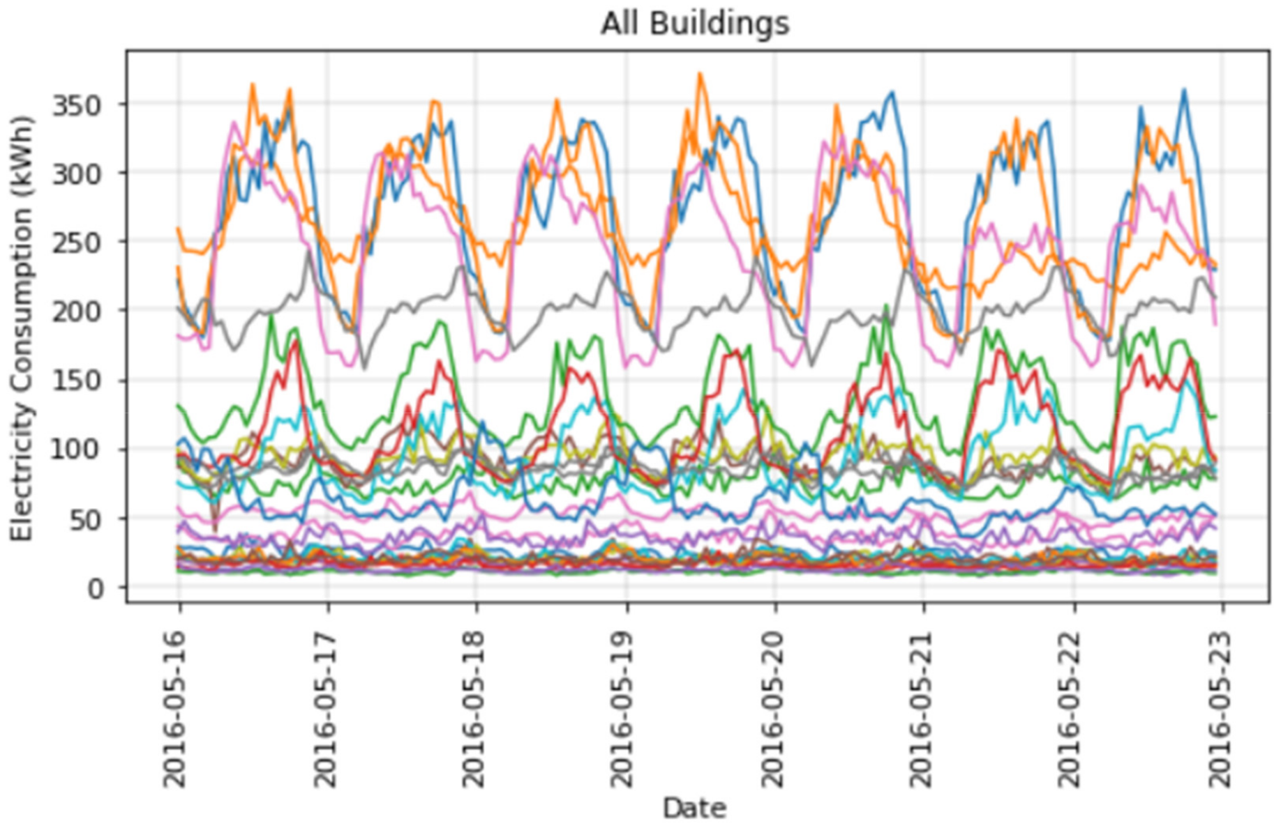
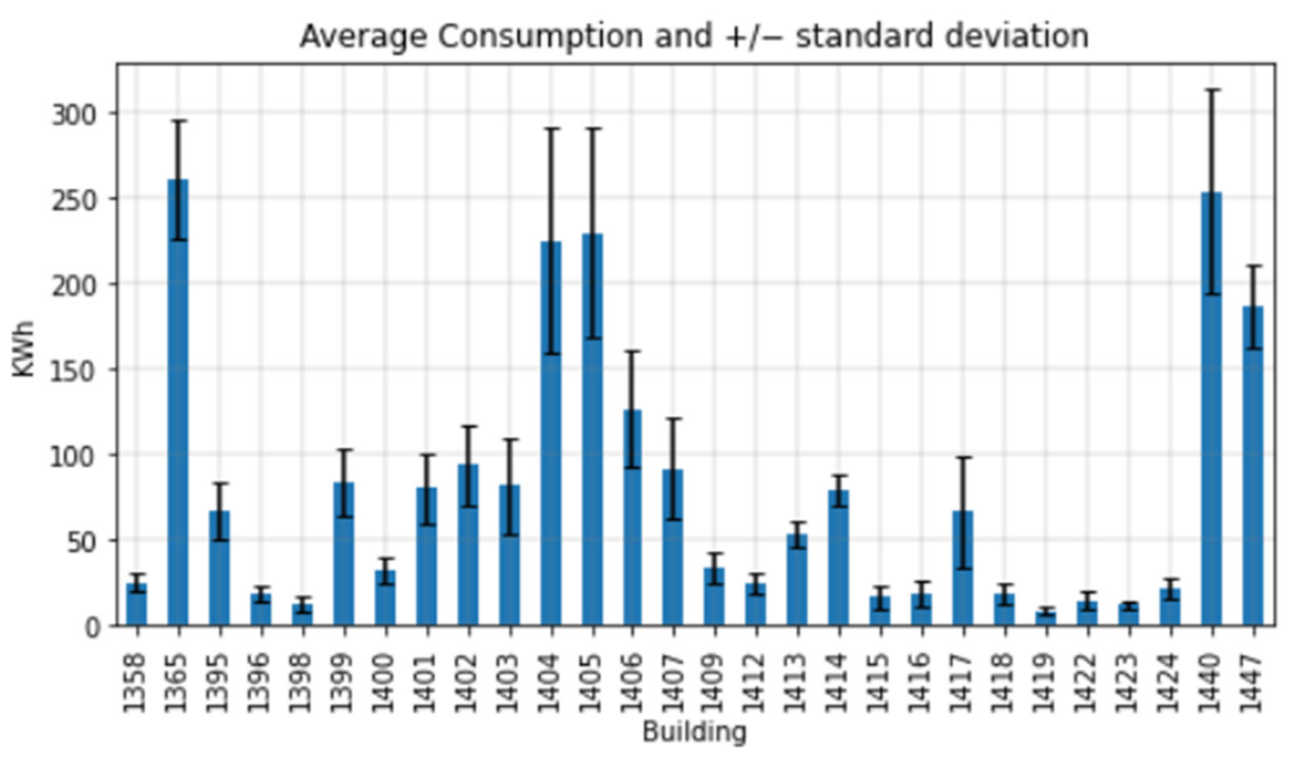
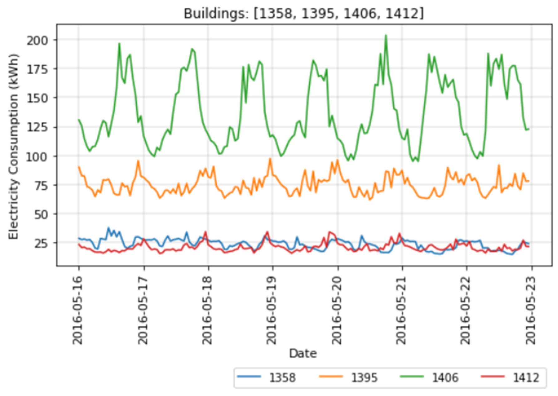
2.2. Dataset Description
2.3. Experimental Setting
2.4. Preprocessing
2.5. Model Training
2.6. Model Performance Evaluation
3. Results
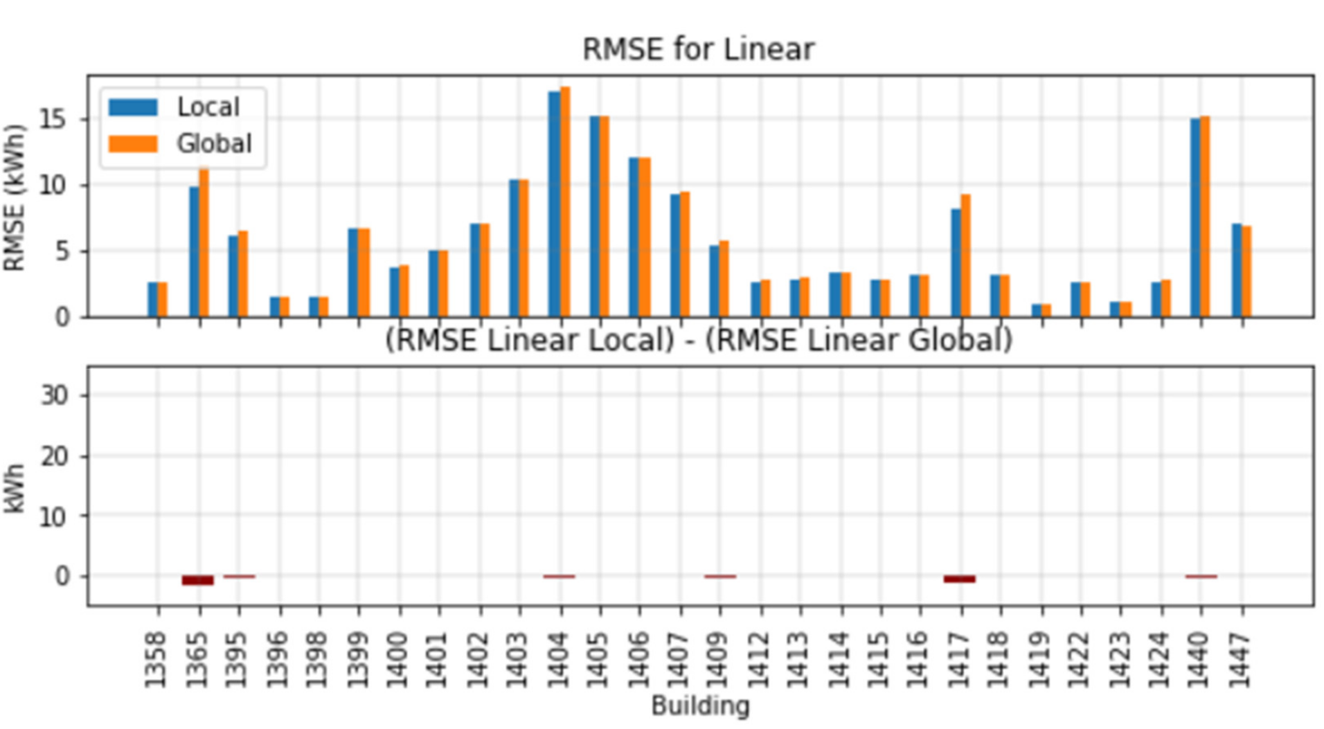
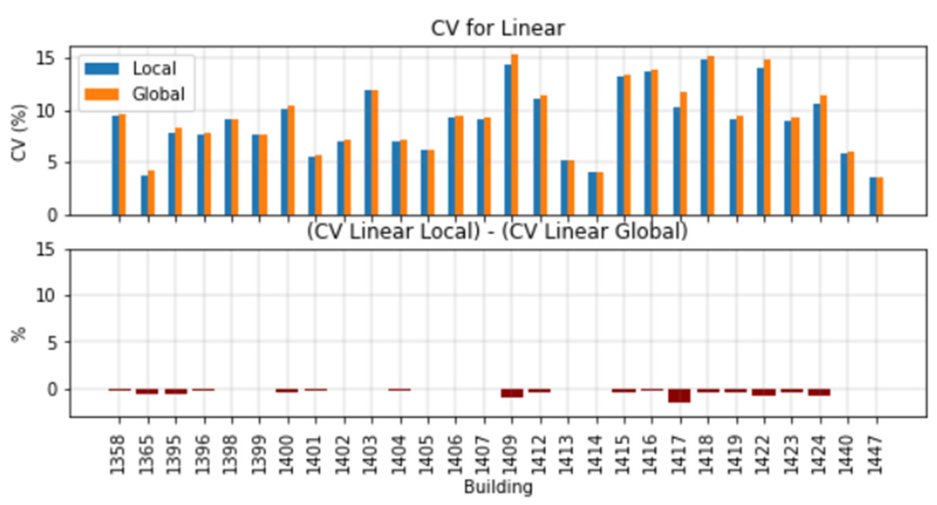
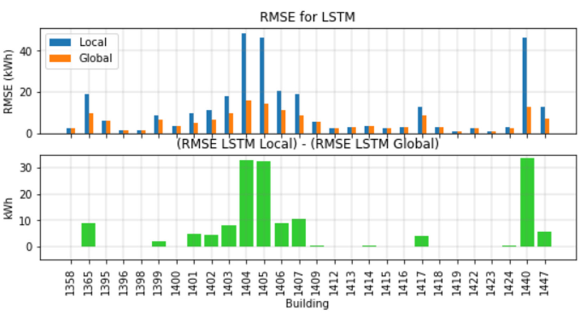
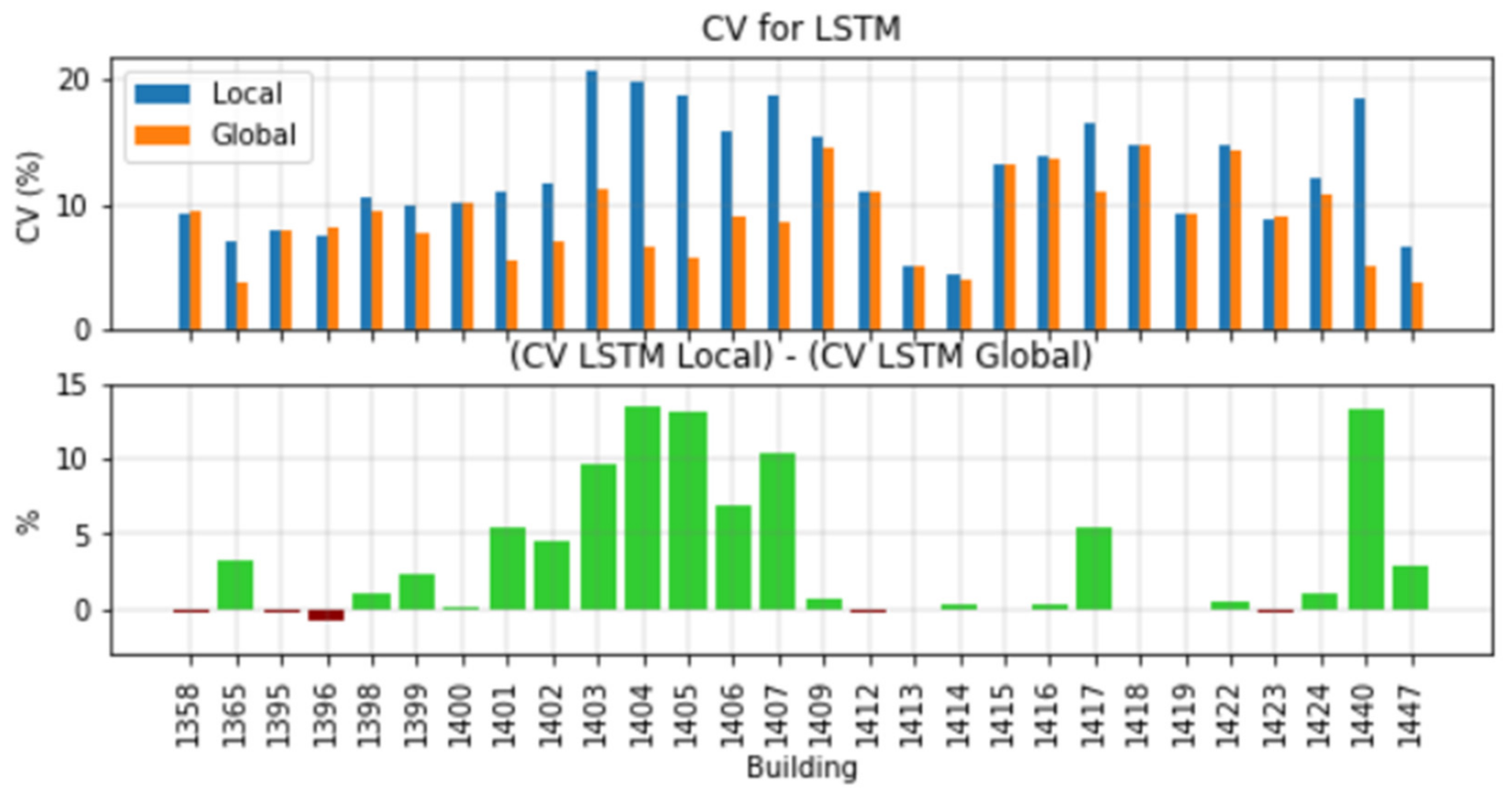
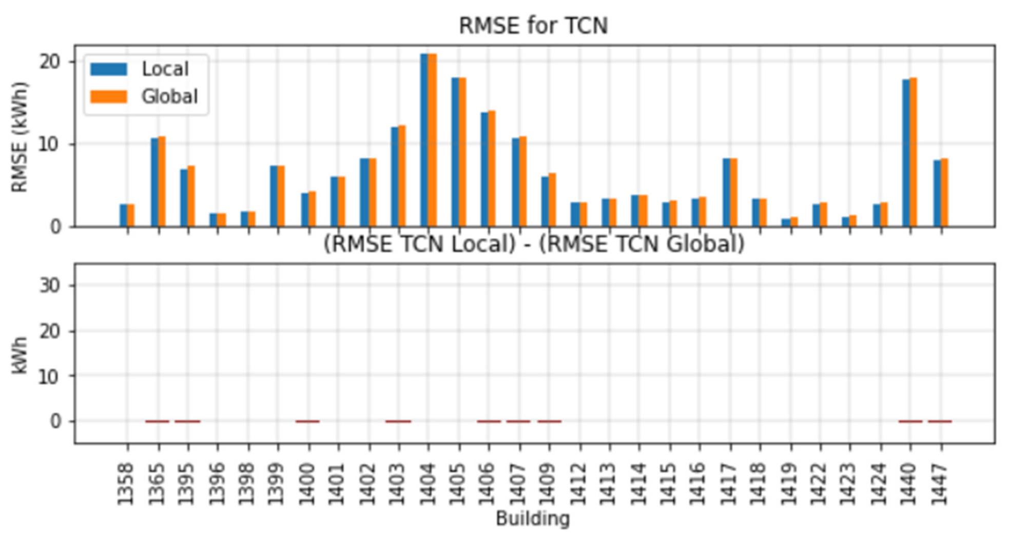
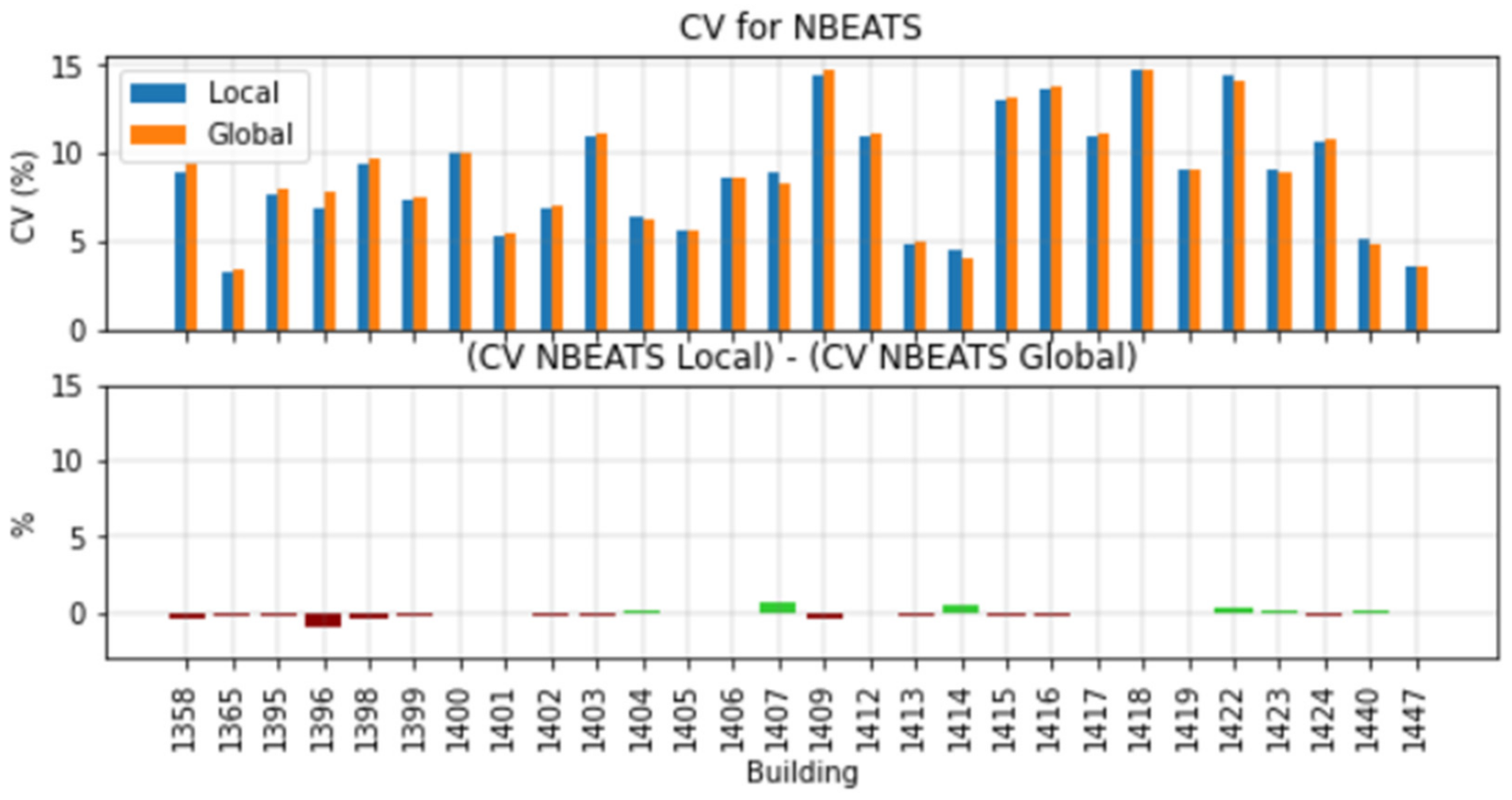
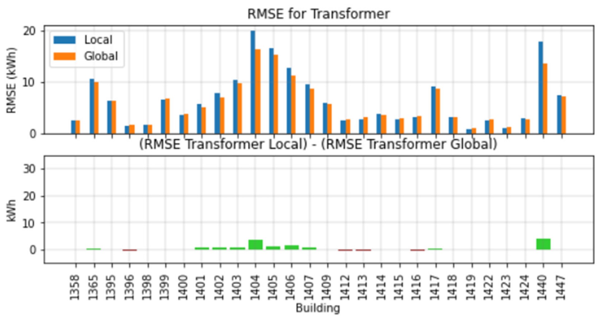
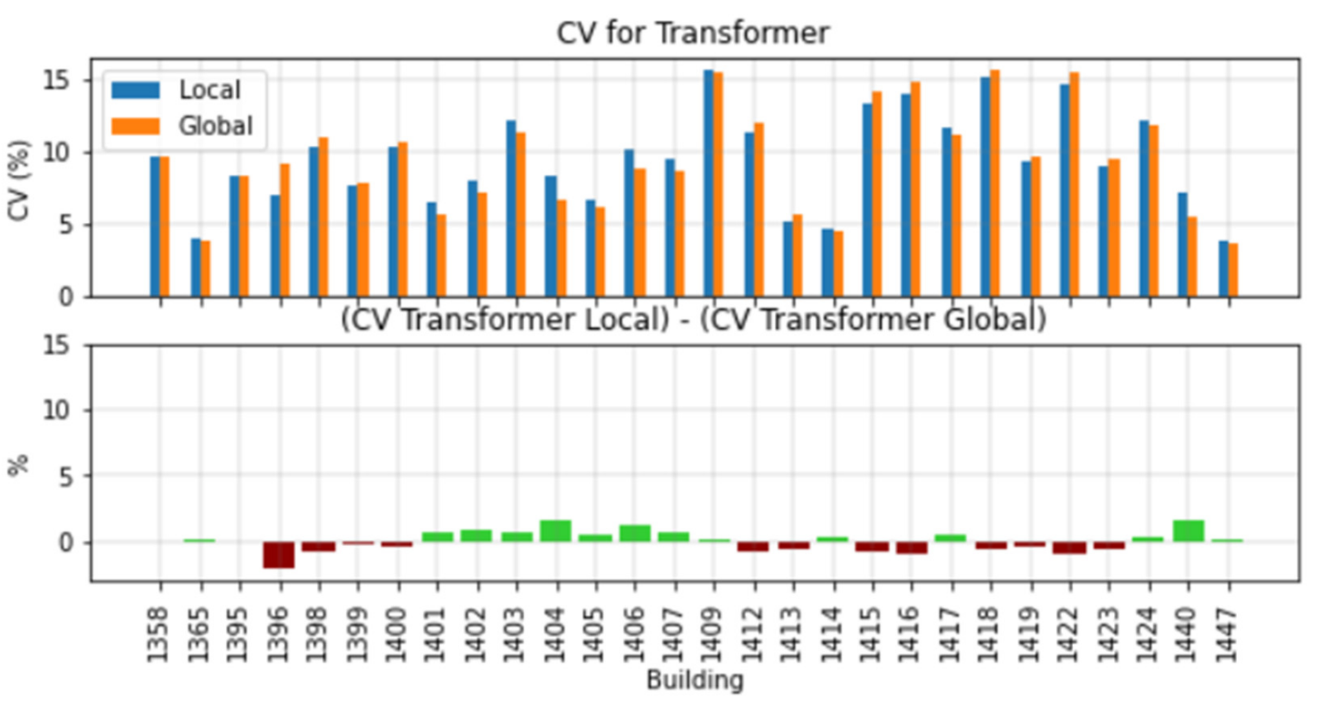
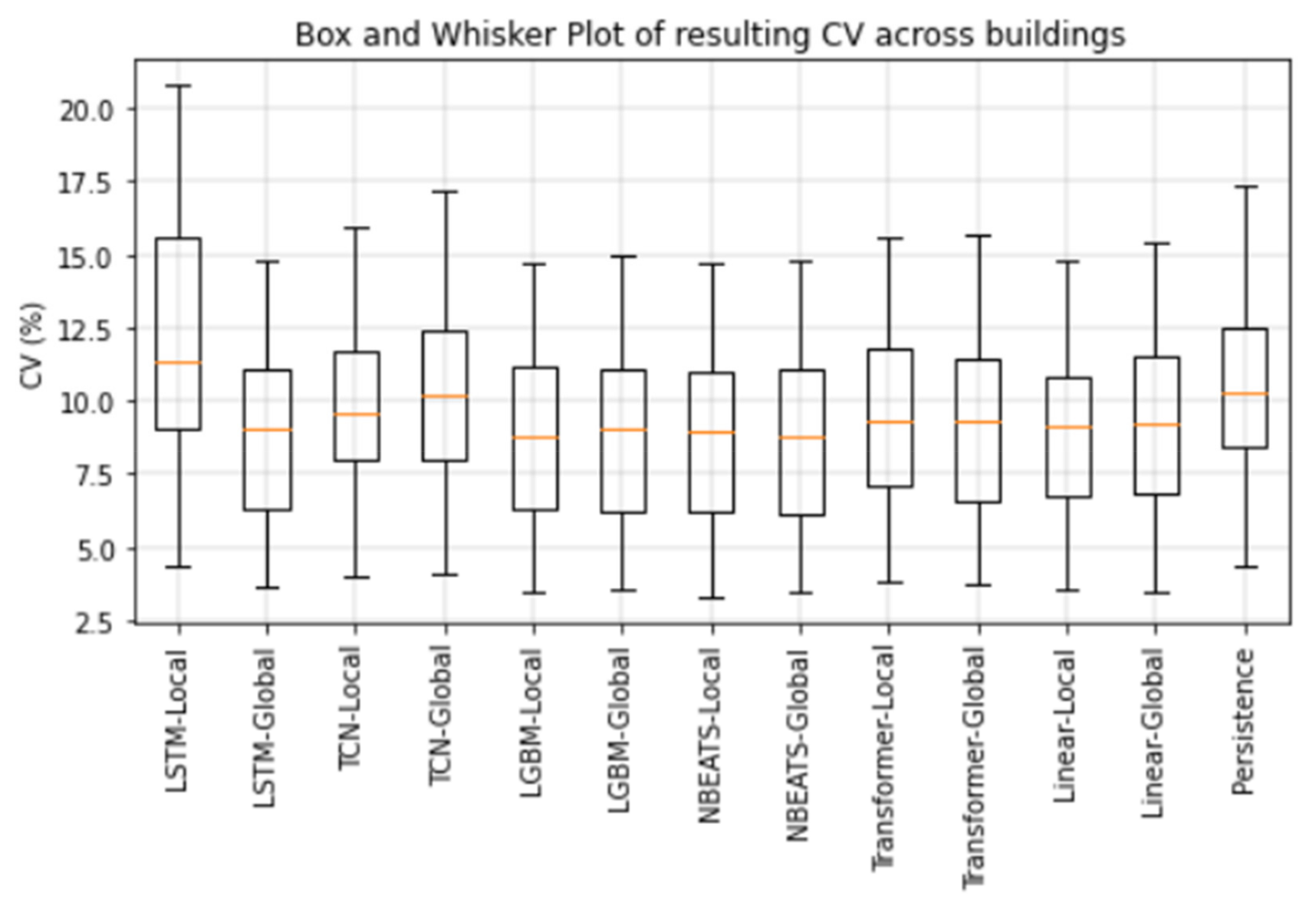
3.1. Comparison between Local and Global Models
3.2. Reuse of Pre-Trained Forecasting Models
4. Discussion
5. Conclusions
Author Contributions
Funding
Institutional Review Board Statement
Informed Consent Statement
Data Availability Statement
Acknowledgments
Conflicts of Interest
References
- IEA. Electricity Market Report; IEA: Paris, France, 2021. [Google Scholar]
- Cao, Z.; Han, X.; Lyons, W.; O’Rourke, F. Energy management optimisation using a combined Long Short-Term Memory recurrent neural network–Particle Swarm Optimisation model. J. Clean. Prod. 2021, 326, 129246. [Google Scholar] [CrossRef]
- Burgio, D.; Menniti, N.; Sorrentino, A.; Pinnarelli, Z.L. Influence and Impact of Data Averaging and Temporal Resolution on the Assessment of Energetic, Economic and Technical Issues of Hybrid Photovoltaic-Battery Systems. Energies 2020, 13, 354. [Google Scholar] [CrossRef] [Green Version]
- Zheng, J.; Xu, C.; Zhang, Z.; Li, X. Electric load forecasting in smart grids using Long-Short-Term-Memory based Recurrent Neural Network. In Proceedings of the 2017 51st Annual Conference on Information Sciences and Systems (CISS), Baltimore, MD, USA, 22–24 March 2017. [Google Scholar]
- Zhao, H.; Magoulès, F. A review on the prediction of building energy consumption. Renew. Sustain. Energy Rev. 2012, 16, 3586–3592. [Google Scholar] [CrossRef]
- Zhang, N.; Li, Z.; Zou, X.; Quiring, S.M. Comparison of three short-term load forecast models in Southern California. Energy 2019, 189, 116358. [Google Scholar] [CrossRef]
- Daut, M.A.M.; Hassan, M.Y.; Abdullah, H.; Rahman, H.A.; Abdullahm, M.P.; Hussin, F. Building electrical energy consumption forecasting analysis using conventional and artificial intelligence methods: A review. Ren. Sust. Energy Rev. 2017, 70, 1108–1111. [Google Scholar] [CrossRef]
- Liang, Y.; Niu, D.; Hong, W.C. Short term load forecasting based on feature extraction and improved general regression neural network model. Energy 2019, 166, 653–663. [Google Scholar] [CrossRef]
- Mandal, P.; Senjyu, T.; Urasaki, N.; Funabashi, T. A neural network based severalhour-ahead electric load forecasting using similar days approach. Elec. Power Energy Syst. 2006, 28, 367–373. [Google Scholar] [CrossRef]
- Shi, H.; Xu, M.; Li, R. Deep Learning for Household Load Forecasting—A Novel Pooling Deep RNN. IEEE Trans. Smart Grid 2018, 9, 5271–5280. [Google Scholar] [CrossRef]
- Zhang, F.; Deb, C.; Lee, S.E.; Yang, J.; Shah, K.W. Time series forecasting for building energy consumption using weighted support vector regression with differential evolution optimization technique. Energy Build. 2016, 12, 94–103. [Google Scholar] [CrossRef]
- Zhang, X.M.; Grolinger, K.; Capretz, M.A.M.; Seewald, L. Forecasting Residential Energy Consumption: Single Household Perspective. In Proceedings of the 2018 17th IEEE International Conference on Machine Learning and Applications, Orlando, FL, USA, 17–20 December 2018. [Google Scholar]
- Kong, W.; Dong, Z.Y.; Hill, D.J.; Luo, F.; Xu, Y. Short-Term Residential Load Forecasting Based on Resident Behaviour Learning. IEEE Trans. Power Syst. 2018, 33, 1087–1088. [Google Scholar] [CrossRef]
- Rafati, A.; Joorabian, M.; Mashhour, E. An efficient hour-ahead electrical load forecasting method based on innovative features. Energy 2020, 201, 117511. [Google Scholar] [CrossRef]
- Abbasi, R.A.; Javaid, N.; Ghuman, M.N.J.; Khan, Z.A.; Rehman, S.U. Short Term Load Forecasting Using XGBoost. In Web, Artificial Intelligence and Network Applications. WAINA 2019. Advances in Intelligent Systems and Computing; Barolli, L., Takizawa, M., Xhafa, F., Enokido, T., Eds.; Springer: Cham, Switzerland, 2019; Volume 927. [Google Scholar]
- Caliano, M.; Buonanno, A.; Graditi, G.; Pontecorvo, A.; Sforza, G.; Valenti, M. Consumption based-only load forecasting for individual households in nanogrids: A case study. In Proceedings of the 12th AEIT International Annual Conference, Web-Conference AEIT, Online, 22–25 October 2020. [Google Scholar]
- Januschowski, T.; Gasthaus, J.; Wang, Y.; Salinas, D.; Flunkert, V.; Bohlke-Schneider, M.; Callot, L. Criteria for classifying forecasting methods. Int. J. Forecast. 2020, 36, 167–177. [Google Scholar] [CrossRef]
- Wagner, N.; Michalewicz, Z.; Schellenberg, S.; Chirac, C.; Mohais, A. Intelligent techniques for forecasting multiple time series in real-world systems. Int. J. Intell. Comput. Cybern. 2011, 4, 284–310. [Google Scholar] [CrossRef] [Green Version]
- Makridakis, S.; Spiliotis, E.; Assimakopoulos, V. The M4 Competition: 100,000 time series and 61 forecasting methods. Int. J. Forecast. 2020, 36, 54–74. [Google Scholar] [CrossRef]
- Makridakis, S.; Spiliotis, E.; Assimakopoulos, V. The M5 Accuracy competition: Results, findings and conclusions. Int. J. Forecast. 2022; corrected proof. [Google Scholar] [CrossRef]
- Laptev, N.; Yosinski, J.; Erran Li, L.; Smyl, S. Time-series Extreme Event Forecasting with Neural Networks at Uber. In Proceedings of the International Conference of Machine Learning, Sydney, Australia, 6–11 August 2017. [Google Scholar]
- Montero-Manso, P.; Hyndman, R.J. Principles and algorithms for forecasting groups of time series: Locality and globality. Int. J. Forecast. 2021, 37, 1632–1653. [Google Scholar] [CrossRef]
- Herzen, J. Training Forecasting Models on Multiple Time Series with Darts. Unit8, 6 July 2021. Available online: https://unit8.com/resources/training-forecasting-models/(accessed on 1 December 2021).
- Hewamalage, H.; Bergmeir, C.; Bandara, K. Global models for time series forecasting: A Simulation study. Pattern Recognit. 2022, 124, 108441. [Google Scholar] [CrossRef]
- Pan, S.J.; Yang, Q. A Survey on Transfer Learning. IEEE Trans. Knowl. Data Eng. 2010, 22, 1345–1359. [Google Scholar] [CrossRef]
- Fan, C.; Sun, Y.; Xiao, F.; Ma, J.; Lee, D.; Wang, J.; Tseng, Y.C. Statistical investigations of transfer learning-based methodology for short-term building energy predictions. Appl. Energy 2020, 262, 114499. [Google Scholar] [CrossRef]
- Mocanu, E.; Nguyen, P.H.; Kling, W.L.; Gibescu, M. Unsupervised energy prediction in a Smart Grid context using reinforcement cross-building transfer learning. Energy Build. 2016, 116, 646–655. [Google Scholar] [CrossRef] [Green Version]
- Ribeiro, M.; Grolinger, K.; El Yamany, H.F.; Higashino, W.A.; Capretz, M.A. Transfer learning with seasonal and trend adjustment for cross-building energy forecasting. Energy Build. 2018, 165, 352–363. [Google Scholar] [CrossRef]
- Ahn, Y.; Kim, B. Prediction of building power consumption using transfer learning-based reference building and simulation dataset. Energy Build. 2022, 258, 111717. [Google Scholar] [CrossRef]
- Wu, D.; Wang, B.; Precup, D.; Boulet, B. Multiple Kernel Learning-Based Transfer Regression for Electric Load Forecasting. IEEE Trans. Smart Grid 2020, 11, 1183–1192. [Google Scholar] [CrossRef]
- Genov, E.; Petridis, S.; Iliadis, P.; Nikopoulos, N.; Coosemans, T.; Massagie, M.; Camargo, L. Short-Term Load Forecasting in a microgrid environment: Investigating the series-specific and cross-learning forecasting methods. J. Phys. Conf. Ser. 2021, 2042, 012035. [Google Scholar] [CrossRef]
- Bai, S.; Kolter, J.Z.; Koltun, V. An Empirical Evaluation of Generic Convolutional and Recurrent Networks for Sequence Modeling. arXiv 2018, arXiv:1803.01271. [Google Scholar]
- Oreshkin, B.N.; Carpov, D.; Chapados, N.; Bengio, Y. N-BEATS: Neural Basis Expansion Analysis for Interpretable Time Series Forecasting. arXiv 2020, arXiv:1905.10437. [Google Scholar]
- Ke, G.; Meng, Q.; Finley, T.; Wang, T.; Chen, W.; Ma, W.; Ye, Q.; Liu, T. LightGBM: A highly efficient gradient boosting decision tree. In Proceedings of the 31st International Conference on Neural Information Processing Systems (NIPS 2017), Long Beach, CA, USA, 4–9 December 2017. [Google Scholar]
- Vaswani, N.; Shazeer, N.; Parmar, J.; Uszkoreit, L.; Jones, A.; Gomez, N.; Kaiser, Ł.; Polosukhin, I. Attention is all you need. In Proceedings of the 31st International Conference on Neural Information Processing Systems (NIPS 2017), Long Beach, CA, USA, 4–9 December 2017; pp. 6000–6010. [Google Scholar]
- Miller, P.; Arjunan, A.; Kathirgamanathan, C.; Fu, J.; Roth, J.; Young Park, C.; Balbach, K.; Gowri, Z.; Nagy, A.D.F.; Haberl, F. The ASHRAE Great Energy Predictor III competition: Overview and results. Sci. Technol. Built Environ. 2020, 26, 1427–1447. [Google Scholar] [CrossRef]
- Sen, R.; Yu, H.F.; Inderjit, D. Think Globally, Act Locally: A Deep Neural Network Approach to High-Dimensional Time Series Forecasting. In Proceedings of the 33rd Conference on Neural Information Processing Systems (NeurIPS 2019), Vancouver, BC, Canada, 10–12 December 2019. [Google Scholar]
- Bandara, K.; Shi, P.; Bergmeir, C.; Hewamalage, H.; Tran, Q.; Seaman, B. Sales demand forecast in e-commerce using a long short-term memory neural network methodology. In Neural Information Processing. ICONIP 2019. Lecture Notes in Computer Science; Gedeon, T., Wong, K., Lee, M., Eds.; Springer: Cham, Switzerland, 2019; Volume 11955. [Google Scholar]
- Herzen, J.; Lässig, F.; Piazzetta, S.G.; Neuer, T.; Tafti, L.; Raille, G.; Van Pottelbergh, T.; Pasieka, M.; Skrodzki, A.; Huguenin, N.; et al. Darts: User-Friendly Modern Machine Learning for Time Series. arXiv 2021, arXiv:2110.03224. [Google Scholar]


| Model Name | Main Chosen Hyperparameters |
|---|---|
| Linear | Fit Intercept: True |
| LSTM | Batch Size: 1024; Hidden Size: 25 Optimizer: Adam with Learning Rate 1 × 10⁻³; Maximum Number of Epochs: 200. |
| TCN | Batch Size: 1024; Dilation: 1; Kernel Size: 3; Number of Filters: 25; Dropout: 0.2 Optimizer: Adam with Learning Rate 1 × 10⁻³; Maximum Number of Epochs: 200. |
| NBEATS | Batch Size: 1024; Number of stacks: 30, Number of blocks: 1, Number of fully connected layers: 4, Number of neurons for each fully connected layer: 256, Expansion Coefficient: 5 Optimizer: Adam with Learning Rate 1 × 10⁻³; Maximum Number of Epochs: 200. |
| LGBM | Number of estimators: 100; Learning Rate:0.1 |
| Transformer | Batch Size: 1024; Dropout: 0.1; Number of multi head attention: 4; Number of encoding layers: 3; Number of decoding layers: 3; Dimension of the feed-forward network model: 512 Optimizer: Adam with Learning Rate 1 × 10⁻³; Maximum Number of Epochs: 200. |
| Model Type | Local (%) | Global (%) | Variation(Local-Global)/Local * 100 |
|---|---|---|---|
| LSTM (*) | 11.29 (9.06, 15.55) | 9.00 (6.31, 11.08) | 8.85 (−0.12, 45.13) |
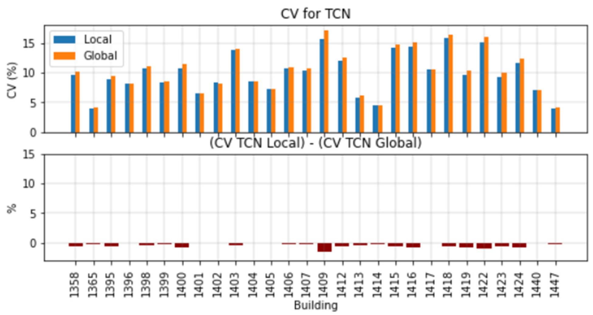
| TCN (*) | 9.58 (7.96, 11.72) | 10.23 (8.01, 12.39) | −3.49 (−5.79, −1.84) |
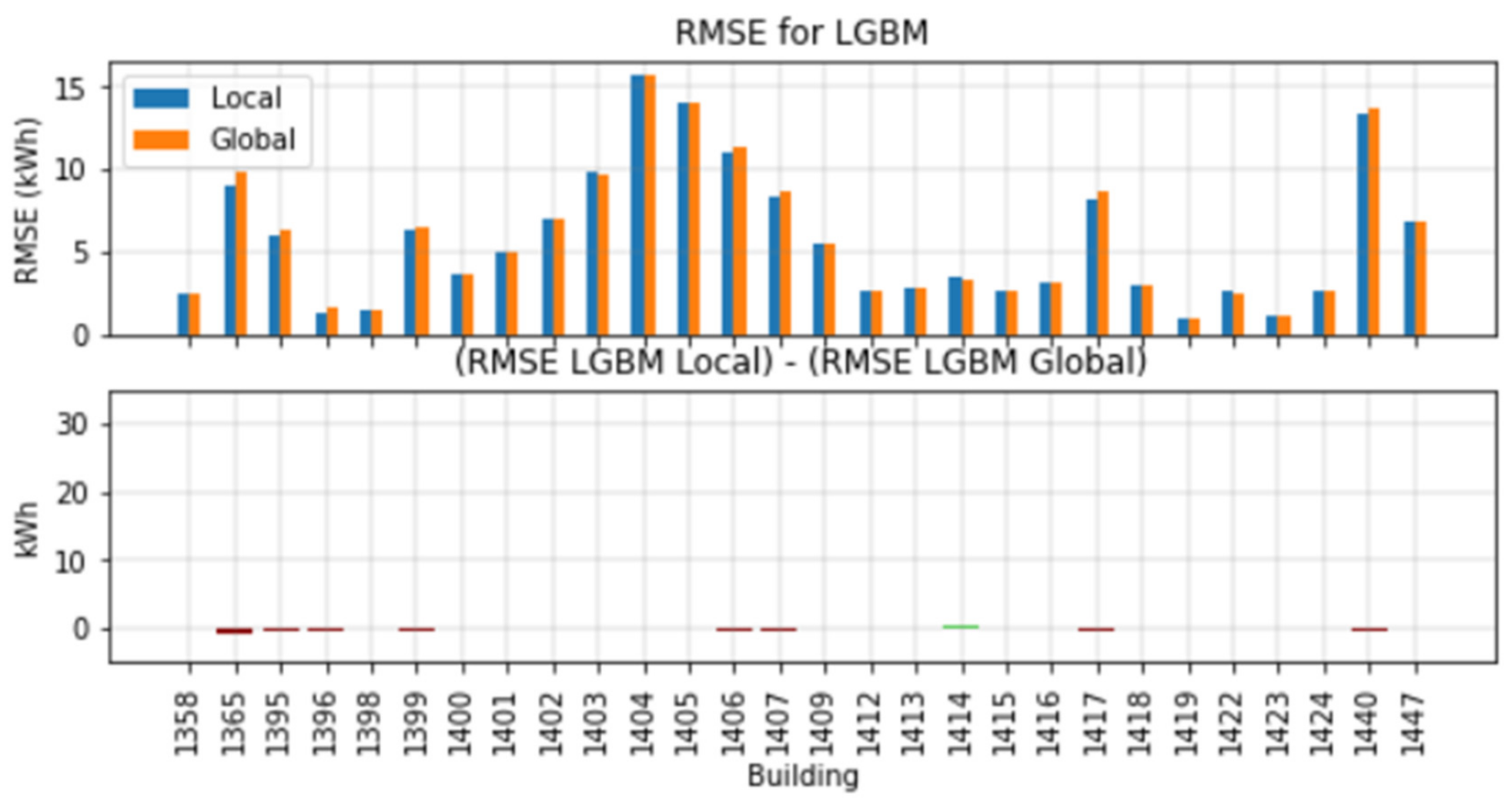
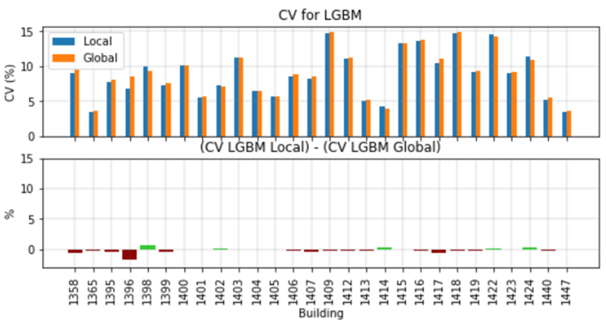
| LGBM (*) | 8.78 (6.25, 11.14) | 9.01 (6.23, 11.10) | −1.09 (−3.67, 0.43) |
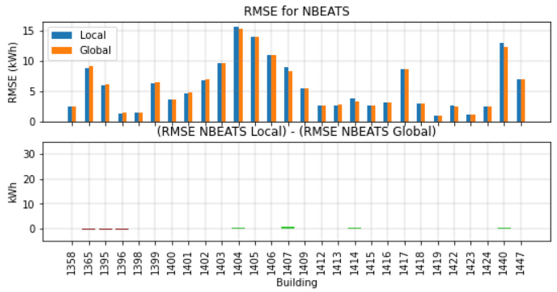
| NBEATS | 8.93 (6.22, 10.98) | 8.73 (6.13, 11.05) | −0.89 (−2.20, 0.59) |
| Transformer | 9.32 (7.07, 11.76) | 9.26 (6.55, 11.45) | 0.16 (−5.44, 6.56) |
| Linear (*) | 9.11 (6.76, 10.76) | 9.23 (6.87, 11.54) | −2.01 (−4.14, −0.69) |
Publisher’s Note: MDPI stays neutral with regard to jurisdictional claims in published maps and institutional affiliations. |
© 2022 by the authors. Licensee MDPI, Basel, Switzerland. This article is an open access article distributed under the terms and conditions of the Creative Commons Attribution (CC BY) license (https://creativecommons.org/licenses/by/4.0/).
Share and Cite
Buonanno, A.; Caliano, M.; Pontecorvo, A.; Sforza, G.; Valenti, M.; Graditi, G. Global vs. Local Models for Short-Term Electricity Demand Prediction in a Residential/Lodging Scenario. Energies 2022, 15, 2037. https://0-doi-org.brum.beds.ac.uk/10.3390/en15062037
Buonanno A, Caliano M, Pontecorvo A, Sforza G, Valenti M, Graditi G. Global vs. Local Models for Short-Term Electricity Demand Prediction in a Residential/Lodging Scenario. Energies. 2022; 15(6):2037. https://0-doi-org.brum.beds.ac.uk/10.3390/en15062037
Chicago/Turabian StyleBuonanno, Amedeo, Martina Caliano, Antonino Pontecorvo, Gianluca Sforza, Maria Valenti, and Giorgio Graditi. 2022. "Global vs. Local Models for Short-Term Electricity Demand Prediction in a Residential/Lodging Scenario" Energies 15, no. 6: 2037. https://0-doi-org.brum.beds.ac.uk/10.3390/en15062037