
Grid-Connected PV System with Reactive Power Management and an Optimized SRF-PLL Using Genetic Algorithm


1
School of Engineering and Physical Sciences, Heriot-Watt University, Edinburgh EH14 4AS, UK
2
Department of Electrical Engineering, Faculty of Engineering Technology, Applied Science Private University, P.O. Box 166, Amman 11931, Jordan
3
Department of Electrical Engineering, College of Engineering Technology, Al-Balqa Applied University, P.O. Box 166, Amman 11931, Jordan
*
Authors to whom correspondence should be addressed.
Energies 2022, 15(6), 2177; https://0-doi-org.brum.beds.ac.uk/10.3390/en15062177
Submission received: 2 January 2022
/
Revised: 23 February 2022
/
Accepted: 14 March 2022
/
Published: 16 March 2022
(This article belongs to the Special Issue Control and Optimization for Energy Management in Smart Grids and Renewable Energy Systems)
Abstract
:This paper presents a two-stage grid-connected PV system with reactive power management capability. The proposed model can send phase-shifted current to the grid during a low-voltage ride through (LVRT) to recover the voltage levels of the grid’s feeders. The novelty of the proposed algorithm, unlike the common methods, is that it does not need to disable the maximum power point tracking (MPPT) state while managing active and reactive power injection simultaneously. Moreover, the new method promotes a safety factor by offering overcurrent protection to the PV inverter. The phase-locked loop based on the synchronous reference frame (SRF-PLL) is optimized using a genetic algorithm (GA). The settling time of SRF-PLL’s step response is minimized, and the frequency dynamics are improved to enhance synchronization during LVRT. The system’s performance is tested and verified using MATLAB/Simulink simulations. The obtained results prove the effectiveness of the proposed control algorithm in managing reactive power interventions. The optimized phase-locked loop shows robust performance and is compared to the conventional low-gain PLL to spot the enhancement.
1. Introduction
Power quality is the capability of an electricity grid to provide customers with resilient, secure, and reliable electricity [1]. Utility grid operators are obliged to follow specific regulations to ensure grids’ stability and retain certain levels of power quality delivered to customers. With more renewable energy generations (REGs) joining the grid, a significant share of the synchronous generation is being displaced without sufficient reactive power compensation being fed into the grid [2]. Therefore, a grid’s voltage control becomes less capable, which imposes more implementation of power quality enhancement technologies to maintain those standards. Some of the developing methods in this regard seek to take advantage of the growing number of REGs. Renewable energy penetration had been adopted as a strategy in many countries across the world, which accounts for almost 35% of the total electricity energy share [3]. The recent grid regulations have paved the way for more distributed generations (DGs) to join the grid and flourish outside the active power boundaries. For instance, recent PV inverters are more capable of contributing to ancillary services to restore a grid feeder’s nominal voltage [4]. It is well known that a grid’s power quality could degrade owing to faults; under similar fault circumstances, it is more practical to utilize DG systems to support the grid rather than disconnecting them. The latter option will put more strain on the utility providers and may shorten the lifespan of DG systems due to frequent restarting. The capability of supporting the grid during voltage sags is called low-voltage ride through (LVRT) [1]. It is usually accomplished by injecting sufficient reactive power into the grid to raise the magnitude of the voltage at the terminals of the point of common coupling (PCC) [5]. A PV system requires a proper control scheme to successfully manage such intervention. The voltage variations within the grid can also influence the performance of the phase-locked loop (PLL).
The impact of voltage disturbances over the PLL have been addressed by many researchers, such as in [6,7,8], where many methods to enhance the frequency and the time responses characteristics of the PLL were proposed. The modified time delay technique was used in [9], in which decent results were obtained; however, the fast-tracking capability under rapid voltage deviations was compromised due to the time delay implementation. Maintaining an acceptable PLL accuracy under rapid changes in the grid’s voltage was addressed in [10], and a second-order generalized integrator phase-locked loop (SOGI-PLL) was suggested to enhance synchronization between the PV system and the connected grid during LVRT. Subsequently, a dual second-order generalized integrator phase-locked loop (DSOGI-PLL) was presented in [11] to enhance the filtration capability of the previously suggested SOGI-PLL. A PLL-less technique was suggested in [12] to avoid the impact of voltage disturbances over PLL accuracy. An arbitrary angle was utilized instead of real-time PLL estimation. However, the drawback of this method was its ability to drop synchronization due to a sudden change in the network’s frequency, and the variable DC bus reference which was suggested led to a reduction in the system’s efficiency. In [13], another PLL-less proposal was presented to make the PV system more resilient against the grid’s faults. The study added a non-linear controller to ensure current protection; however, both MPPT performance and DC bus stability were not addressed. In [2], the authors suggested utilizing a battery to stabilize the DC bus voltage, but the study did not discuss the case of insufficient battery charge. A control strategy in a double-stage PV inverter’s topology was proposed in [14] to support the grid during LVRT. The methodology included two states of operation: one under a normal condition and another under a faulty condition. The faulty condition required MPPT to be disabled to allow reactive power injection to the grid. A predictive control technique was suggested in [15,16,17] to provide robust performance in both stand-alone and grid-connected operations. The predictive control scheme in the controller managed to provide an LVRT capability by injecting reactive power; however, the authors did not address the current limitation which is critical in such a scenario. In [18], an improved methodology to inject reactive power to the grid was proposed, but the inverter’s current limiter was not part of the discussion.
The proposed model in this paper aims to provide an all-around solution by introducing a novel control scheme that manages active and reactive power injection simultaneously and an optimized synchronous reference frame PLL based on the genetic algorithm to enhance the synchronization between the PV system and the connected grid under rapid voltage deviations. Having discussed the relevant literature, the rest of the study is structured as follows: Section 2, materials and methods; Section 3, simulations and discussions; and Section 4, conclusions.
2. Materials and Methods
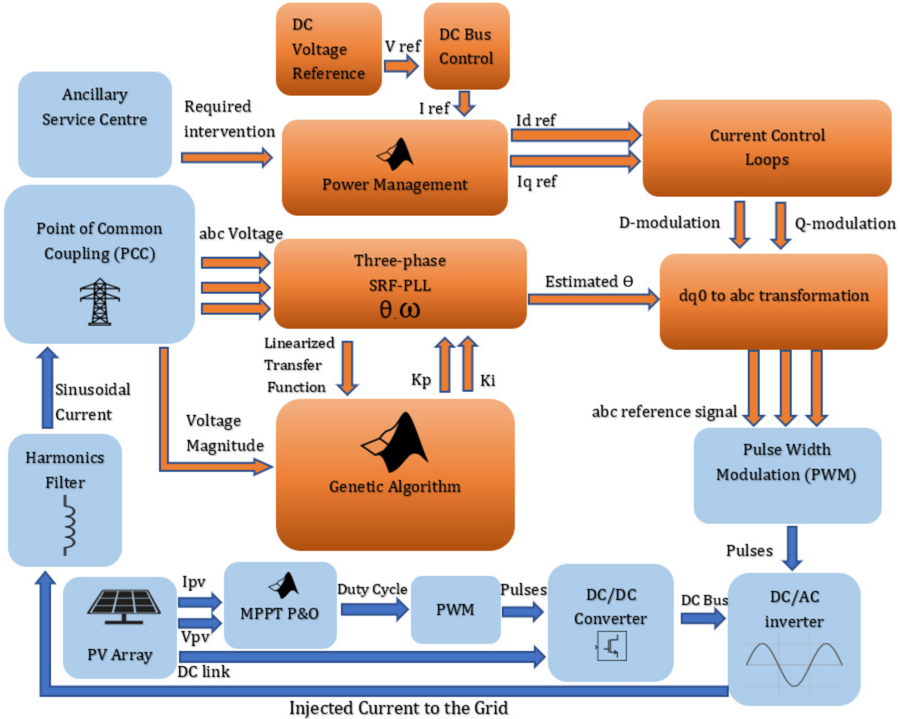
A two-stage boost converter topology is employed in this paper as the power conversion tool of the user-defined PV array (17 parallel strings and 14 series modules per string) with total power capacity of 50 kW. One of the key benefits of this topology is that it allows for more variables to be controlled than a single-stage topology [19]. This results in several control loops for various objectives, such as a DC bus voltage regulation control loop, inverter’s currents control loops, and the MPPT algorithm [20]. The proposed power management unit is fitted prior to current control loops to offer the system an LVRT functionality, while a GA algorithm is utilized to optimize the transfer function of the SRF-PLL for better performance under LVRT. The boost converter is the initial stage of this power conversion topology. To stabilize the converter’s output voltage, a PI controller is used, while a perturb and observe MPPT algorithm is utilized to control the switching gates of the power transistors. Both the DC voltage and current control loops and the optimized SRF-PLL are visually illustrated through schematics and explained arithmetically in this section. The main goal of the designed inverter’s control system is to stabilize the DC bus voltage while injecting the desired current to the grid. As a result, the system provides the grid with the appropriate amount of active power based on the available power extracted from the PV panels and the appropriate amount of reactive power based on the utility’s needs. A simplified schematic of the proposed model is illustrated in Figure 1:
2.1. Synchronous Reference-Frame-Based Phase-Locked Loop (SRF-PLL)
The phase-locked loop is a vital part of the grid-connected PV system; its performance under different grid conditions has an instrumental impact over the PV system output signals. Both active and reactive power injection depend on the accuracy of the SRF-PLL’s phase estimation of the grid’s voltage. The arithmetic model of SRF-PLL is constructed to analyze the time response and the frequency dynamics of the SRF-PLL’s transfer function. The analysis is followed by a study to demonstrate the usefulness of the genetic algorithm (GA) to optimize the settling time of the step response. In addition, the importance of including a constraint function within GA to retain certain frequency characteristics is highlighted. Despite the fact that the PLL system’s bandwidth is increased, the analysis does not include a low pass filter (LPF), because adding a LPF to the loop filter decelerates phase tracking capabilities [21]. The utility voltage is the SRF-PLL’s input signal, which initially is transformed from the natural frame abc to the synchronous reference frame dq0 using park transformation. The direct and quadrant components of the utility voltage can be described as follows:
which yields the following:
where is the angle of the input signal, is the angle of the output signal, and are the direct and quadrant components of the synchronous reference frame, respectively, and the zero sequence is zero as the grid is assumed to be balanced, i.e., . The system is not linear by nature due to the park transformation applied to its input signal. However, we can linearize it close to the locking state where input and output frequencies are the same. In other words, and the error angle is very small, thence the following assumption will become valid: Accordingly, the forward path input signal becomes:
with U being the input line to neutral peak voltage. The open-loop transfer function of the error signal, , can then be written as in Equation (4):
where h(s) is the transfer function of the PI controller:
The open-loop transfer function of the error signal can be found by substituting Equation (5) in (4), which yields:
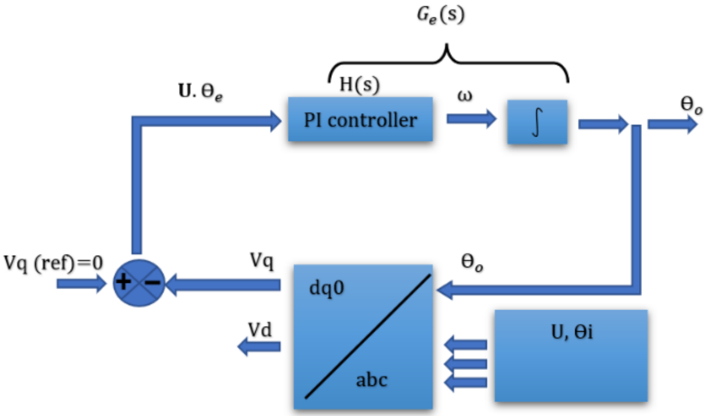
The error signal’s linearized closed-loop transfer function is obtained by passing the estimated output angle back to the (abc-dq0) transformation block as an angular displacement of the synchronous frame, as illustrated in Figure 2 and expressed in Equation (7):
As a result, the PLL transfer function will have the following characteristic equation:
Using Equation (9), which represents the standard second-order characteristic equation as a reference, the correlations between on one side and the corner frequency and the damping ratio ξ on the other side are defined in Equations (10) and (11):
Both frequency and damping ratio values can be modified by altering the gain controllers (). This defines frequency features such as bandwidth ‘’, gain, and phase margins; the same method can be also used to modify time response characteristics such as settling time, rise time, and overshoot [22]. Both frequency and time responses optimization techniques can be used to optimize the final transfer function; in this work, both types of characteristics are considered. However, for an optimization method that is completely dependent on the controller gains regulations, it is crucial to define a range of values where the transfer function is fast and accurate without sacrificing its stability or performance. The obtained range will also help minimize the search time as the gains’ selection process is more confined. Different PLL designs can be derived by altering frequency and time characteristics. For instance, high and low bandwidth can be obtained by modifying the corner frequency , while under-damped and over-damped responses can be achieved by adjusting the damping ratio . The high-bandwidth PLL features fast tracking capability, but due to vast frequency spectrum through-transmission, it may suffer from harmonics [23]. A low bandwidth, on the other hand, is more suitable for filtering out harmonics from the input signal, but it lacks precision when dealing with instable inputs [24]. Both requirements cannot be satisfied simultaneously because the two conditions are inconsistent [24]; therefore, a trade-off is inevitable in the final design. High bandwidth transfer function is preferable here, since it features quick and accurate detection of the phase under grid’s voltage disturbances [25]. This feature will be beneficial during a low-voltage ride through LVRT condition, as the SRF-PLL needs to track the utility’s angle when the voltage amplitude is rapidly changing. To avoid any under or excess damping, a suitable damping ratio is also required; such a value is between 0.7 and 1 [24]. The high bandwidth is achieved by implementing low boundaries for the integral gain Ki, while an acceptable range of damping ratio is maintained by including a constraint function within the optimization method to satisfy the following non-linear conditions:
The settling time of the PLL step response is selected as the search method’s objective value. The rationale for this is that the settling time of the PLL’s step response represents the time required by the SRF-PLL to reach the steady state or to settle close to it after a jump in the utility voltage, making this criterion an ideal candidate to be used as an objective in the case of utility’s voltage disturbances. With this strategy, a successful optimization should result in a robust and resilient performance against voltage sags.
2.2. Implementation of Genetic Algorithm
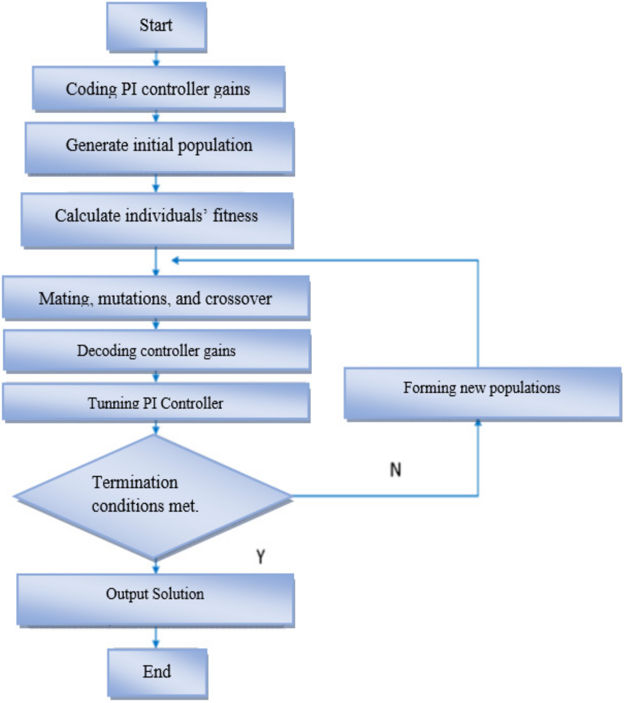
A genetic algorithm (GA) is a random searching method that is well suited to solve non-linear problems; the method uses probabilistic over deterministic fundamentals in a way that mimics natural evolution to find the optimal potential solution [26]. Initially, the problem variables are coded; those variables are called individuals, a group of individuals are called generation, and binary coding of individuals stands for chromosomes. Similarly, procedures such as mating reproduction and mutation are applied within individuals of each generation; the whole cycle is called an iteration. The GA determines the fitness of each individual based on their objective score within a fitness function [27]. In this study, the step response of the PLL transfer function is considered as the fitness function, and the resulting settling time is the objective score; the gains of the loop filter and represent the targeted individuals, as illustrated in Figure 3.
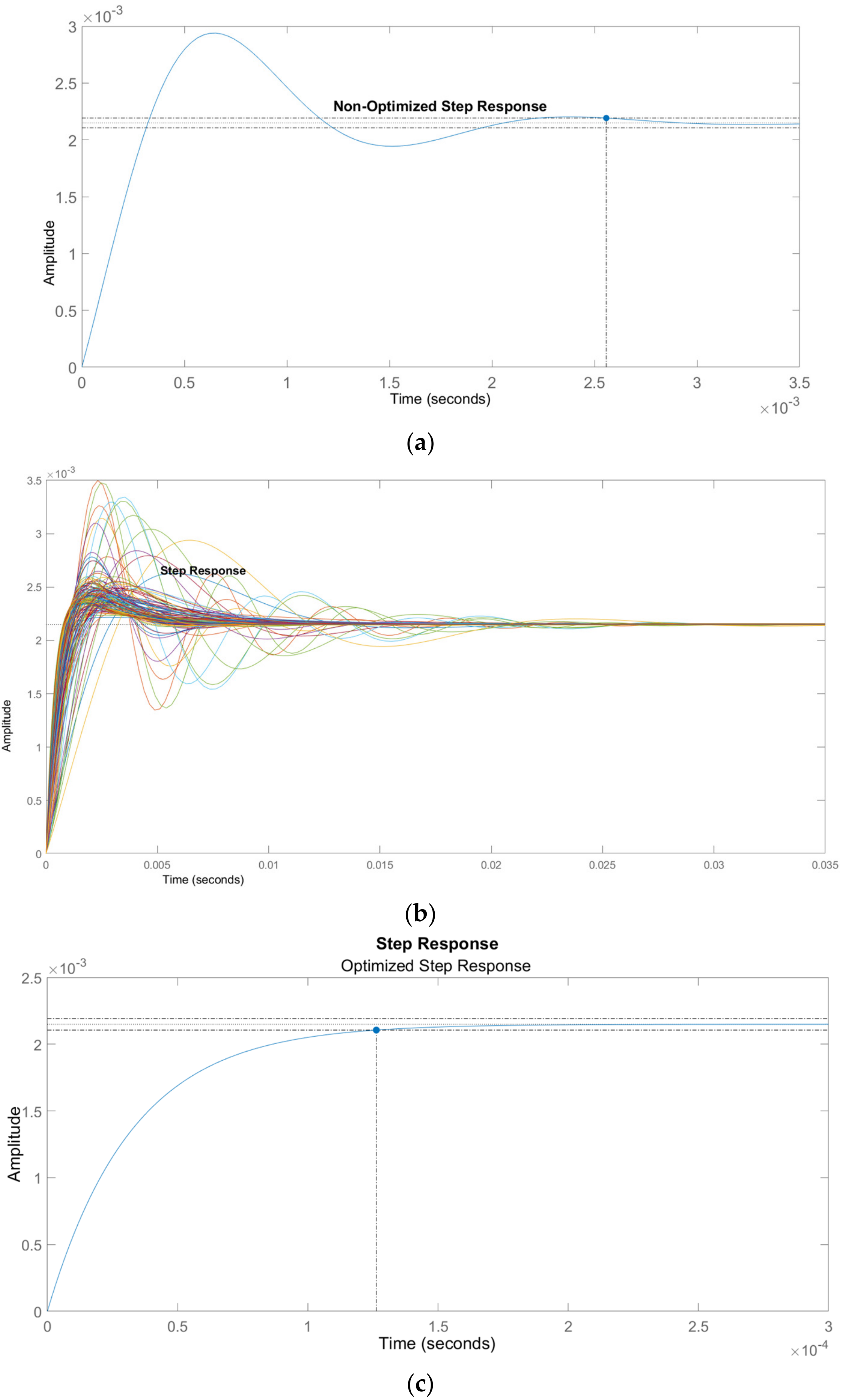
The initial individuals are created at random and coded; the associated settling time of the first pair is acquired by stepping the transfer function, as depicted in Figure 4a. The optimization process takes place as different combinations of Kp and Ki, are enhanced genetically based on their objective score; the same is illustrated in Figure 4b.
The GA converges with the minimum settling time found, as seen in Figure 4c; this occurs once any of the GA solver termination conditions are satisfied, which could be a tolerance of the settling time change, a maximum number of generations, or simply a time limitation. Utilizing suitable termination conditions helps to dramatically minimize the search time without compromising the objectives. The desired frequency characteristics in terms of damping ratio and corner frequency are also satisfied through implemented integral gain boundaries and constraint function. The mathematical rules that govern the constraint function can be found by substituting Equations (10) and (11) in Equations (12) and (13):
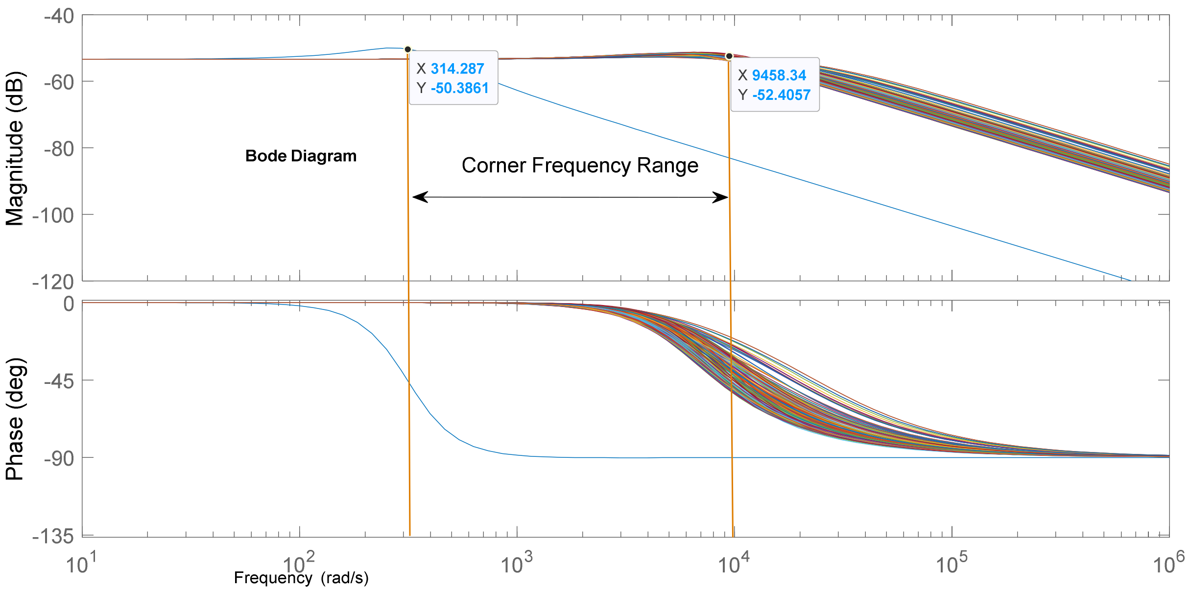
Bode diagrams of different transfer functions are depicted in Figure 5; these transfer functions satisfy the previously mentioned Equations (14) and (15) and feature high-frequency bandwidths between 314 r/s and 9400 rad/s.
The transfer function obtained using this method attributes fast dynamics due to a high frequency range, a proper damping ratio (0.7 to 1), and a minimized settling time. The converged transfer function varies with different criterions being considered. The considered criterions within this exact search method are shown below in Table 1:
2.3. DC Voltage Control Loop
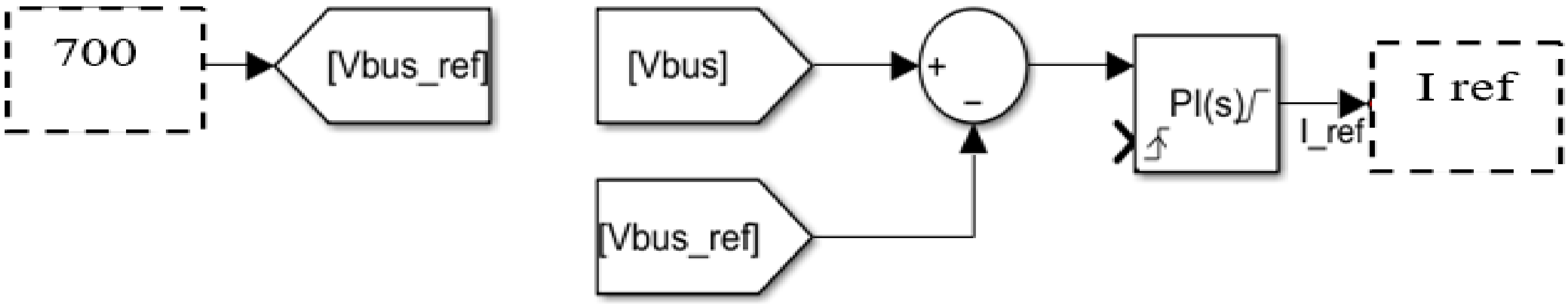
To stabilize the dc-link capacitor’s voltage as per reference value, a DC bus voltage regulation loop is necessary; the gains of the loop filter are tuned using a trial-and-error method; the schematic of the DC voltage controller is illustrated in Figure 6:
The output of PI controller in the DC bus voltage control loop is , which is used as a reference value of the direct current () in the current’s control loops can be expressed by means of controller gains, as demonstrated in Equation (16):
where is the measured voltage across the DC bus capacitor, and is the reference value of the DC bus voltage that must exceed the peak value of the utility voltage, which is between 600 and 1000 volts for a three-phase topology [28]. The settling time of the DC control loop should be longer than that of the two inner current control loops [18], and the gains’ selections should reflect this design condition.
2.4. Current Control Loops
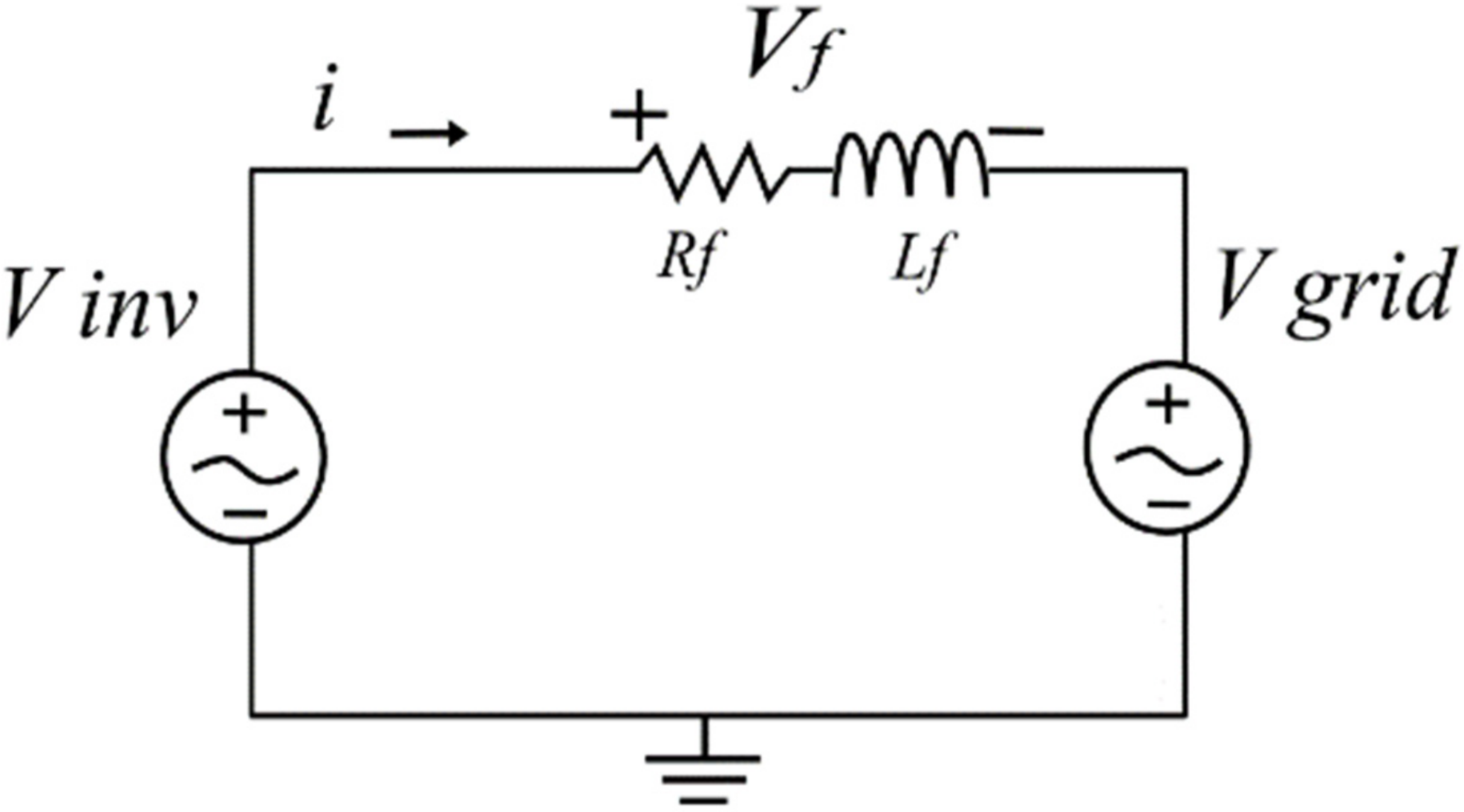
While the DC bus voltage is regulated by the outer control loop, the inverter’s current is regulated by the two inner control loops. To demonstrate the layout of these loops, the inverter’s voltage equation is introduced in Equation (17), which represents the inverter’s voltage in terms of grid and filter voltages, as shown in Figure 7.
where is the inverter’s voltage, is the grid’s voltage, and is the voltage drop across the harmonics filter. The two components of the filter’s voltage and are given by Equations (18) and (19):
where and are the components of the inverter’s current, and and are their reference values, respectively, is the filter’s inductance, is the ohmic resistance of the filter, and represents the inductive reactance. Equations (18) and (19) can be expressed by means of controller, as depicted in Equations (20) and (21).
The two components of the inverter’s voltage in the frame and can be expressed as in Equations (22) and (23).
where and are the components of the grid’s voltage; substituting Equations (20) and (21) in (22) and (23) will yield the following two equations:
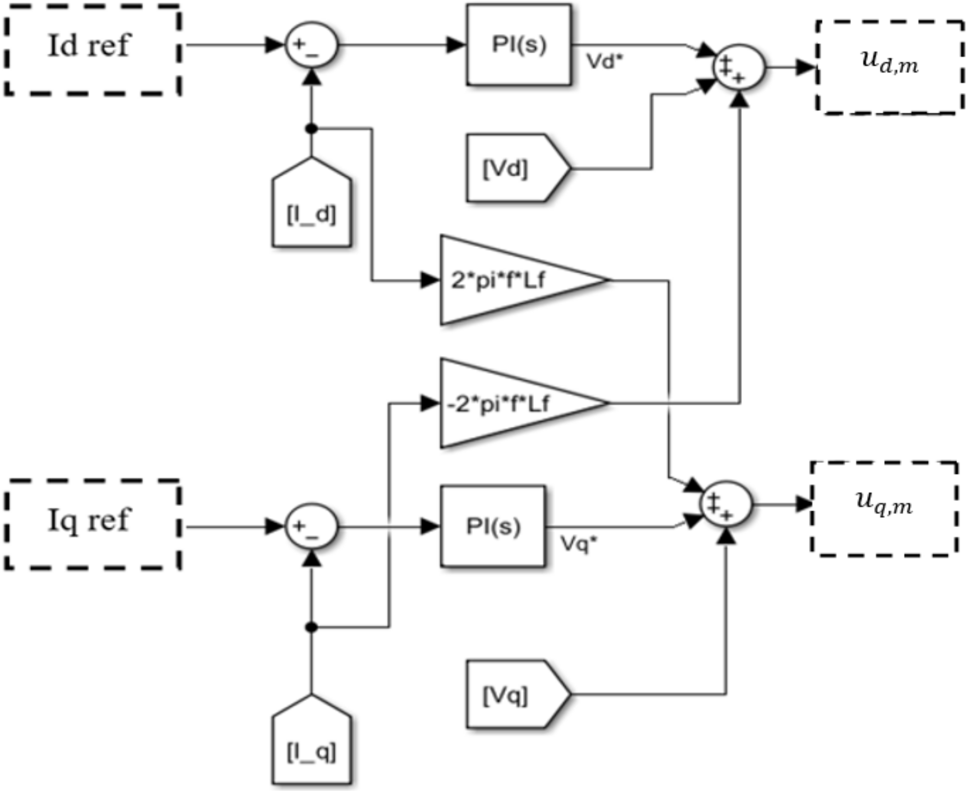
The output signals of the current control loops in the frame represents the components of the inverter’s voltage. These are referred to as and in Figure 8, which highlight their rule as modulation signals, whereby the reference values for both the direct and quadrant currents are imported from the power management unit. A reverse park transformation is used to transfer the modulation signals from the to the natural abc frame, and the resulting signal is used as the reference voltage in the PWM circuit. controllers of the inner current control loops are utilized to regulate the error signal between and their reference values , , whereby both references are generated through the power management unit (PMU). The output signal of the outer control loop “ ” in Equation (16) is used as the reference value of , while is assigned to zero in the case of normal condition and has a non-zero value in the case of LVRT intervention.
2.5. Reactive Power Management
Different methods and strategies can be found in the literature, but the most distinguishing feature of the proposed strategy is that it prioritizes active power injection as a primary system objective above reactive power injection as a secondary system objective. Another modification is the removal of two PI controllers from the inverter’s control scheme, which are typically included for P and Q loops. Alternatively, the reference values of the direct and quadrant inverter’s current components that correspond to the desired PQ flow is generated by the algorithm. The advantage of such scheme is the efficiency gained due to its enabled MPPT and the current protection due to the implemented over-current constraints. The underlying fundamental principle of the proposed algorithm is simple: keep the system operating under the MPPT state and only interfere when you can and when it is needed. The margin of intervention is constrained by the available current, which separates the inverter from reaching its maximum rated limit. The calculated required quadrant current is compared to the available margin; if it is less than the latter, then the intervention is fully served, but otherwise, the maximum possible intervention is applied. The system reduces or even terminates the process once the margin is claimed back partially or fully to support the MPPT state or if the service is no longer needed. The flowchart of the proposed algorithm is depicted in Figure 9, showing how the system responds to ancillary services while maintaining the ongoing MPPT state.
Arithmetically, the decoupled active and reactive power can be expressed by means of inverter’s current and grid’s voltage components as in Equations (26) and (27).
where P and Q are the active and reactive power injected into the grid, respectively. The required value of the quadrant current component represents the required reactive power, and it is calculated using Equation (28).
is zero when the estimated angle by SRF-PLL is being used as the angular displacement of the ‘abc’ to ‘dq0’ transformation. The output of the voltage regulator is assigned as the reference value of the direct current , which reflects a continuous MPPT state.
Therefore, the system always injects the power of the maximum power point . Alternatively, the available marginal quadrant current is calculated using Equation (30).
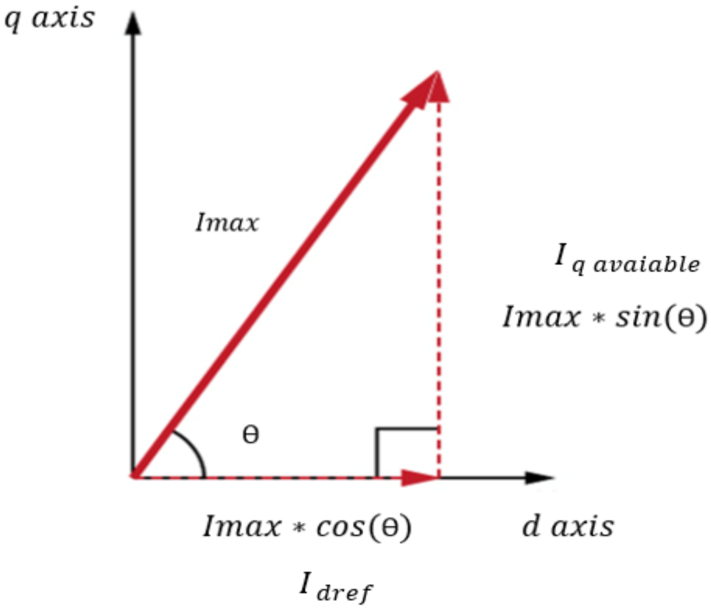
where represents the inverter’s rated current. The former equation represents the trigonometric relation between three components , which is illustrated in Figure 10, where is the needed displacement angle between the inverter’s current and the grid’s voltage.
The following logical statements govern the process of determining the quadrant current reference value .
When
Finally, to calculate the required quadrant current , the value of reactive power should be known. To accomplish that, the magnitude of the voltage sag is first calculated using Equation (33) [29].
The maximum apparent power that can be exported by the inverter is (), which is given by Equation (34) [29].
The required compensational percentage (), which is a function of voltage sag, is given by Equation (35) [15].
Equation (35) reflects specific grid regulations [15], and different grid operators might indicate different requirements. The required reactive power can be calculated accordingly using Equation (36).
Eventually, can be calculated using Equation (28). The proposed algorithm generates a suitable reference value to the inverter’s quadrant current based on Equations (31) and (32) so the system can manage the intervention. Alternatively, to receive the required intervention directly through an automated ancillary service request, which is assumed to be the case here, is calculated directly using Equations (31) and (32) without the need of voltage sag calculations.
3. Simulations and Discussions
In this section, Simulink simulations are utilized to verify the performance of the optimized SRF-PLL and the proposed power management algorithm. The corresponding results are discussed in context. Starting with the phase-locked loop capability of fast-tracking dynamics under voltage disturbances and harmonics, the obtained performance results of the optimized phase-locked loop are discussed and compared to a conventional low-gain PLL to spot the enhancement and potential trade-offs. The suggested reactive power management method during a low-voltage ride through (LVRT) is tested. The grid-connected PV system behavior during the nominal condition and reactive power compensation is illustrated. The MPPT continuity and overcurrent protection features are also presented and discussed.
3.1. SRF-PLL Simulations and Discussions
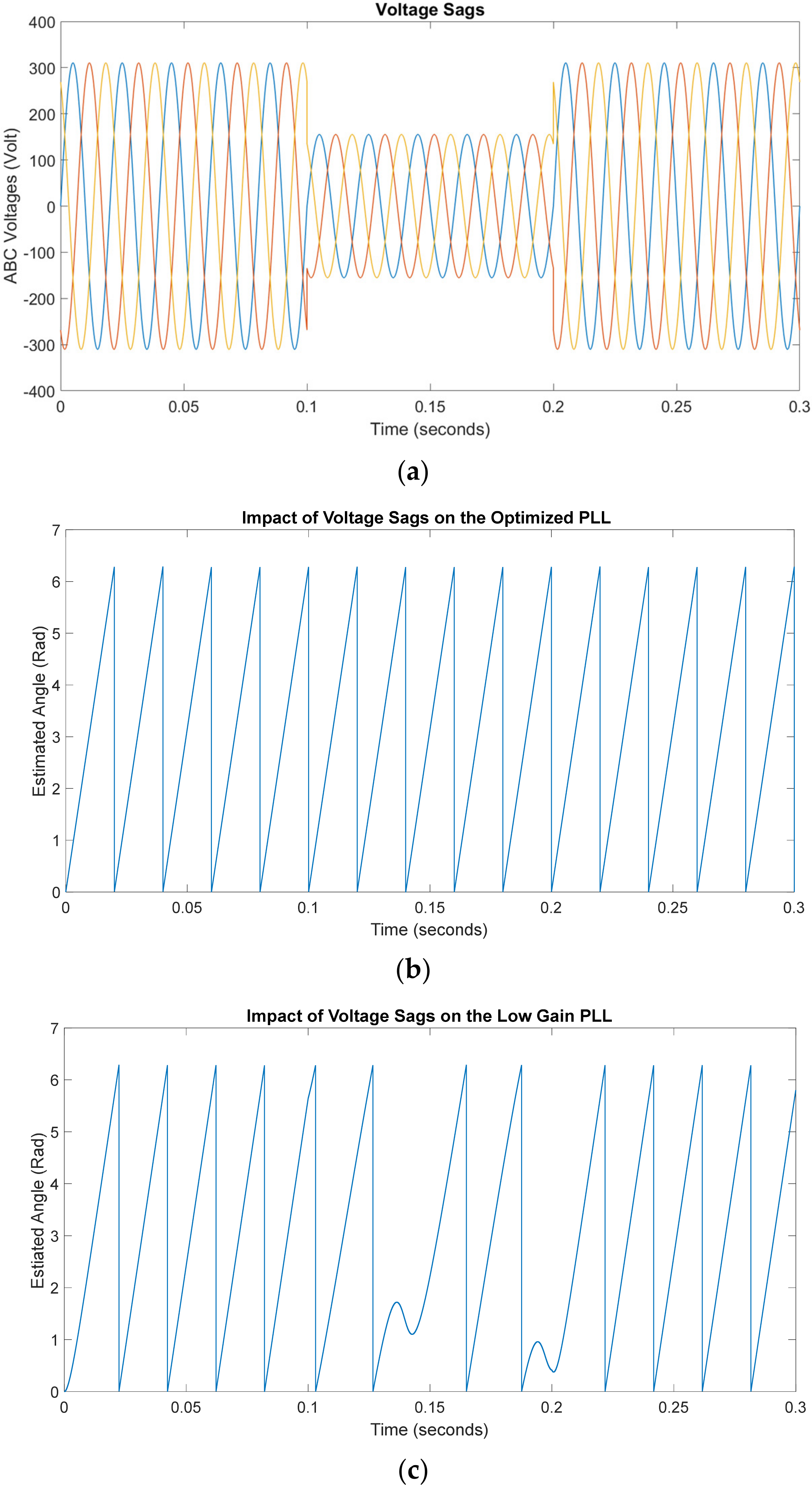
To benchmark the performance of the SRF-PLL under the LVRT condition, the input signal is altered in terms of frequency and voltage values; similar verification methods were used in the literature, such as in [30,31]. The magnitude of the utility’s voltage is reduced to 50% pu between 0.1 and 0.2 s, which corresponds to five cycles. As shown in Figure 11a, this is carried out to verify the performance of the phase-locked loop against voltage sags. The performance of the optimized SRF-PLL is shown in Figure 11b, and the low-gain SRF-PLL performance is shown in Figure 11c. The low-gain phase-locked loop produced distortion in phase estimation. Conversely, the genetically tuned SRF-PLL is resistant and gives robust performance due to the fast dynamics of its transfer function.
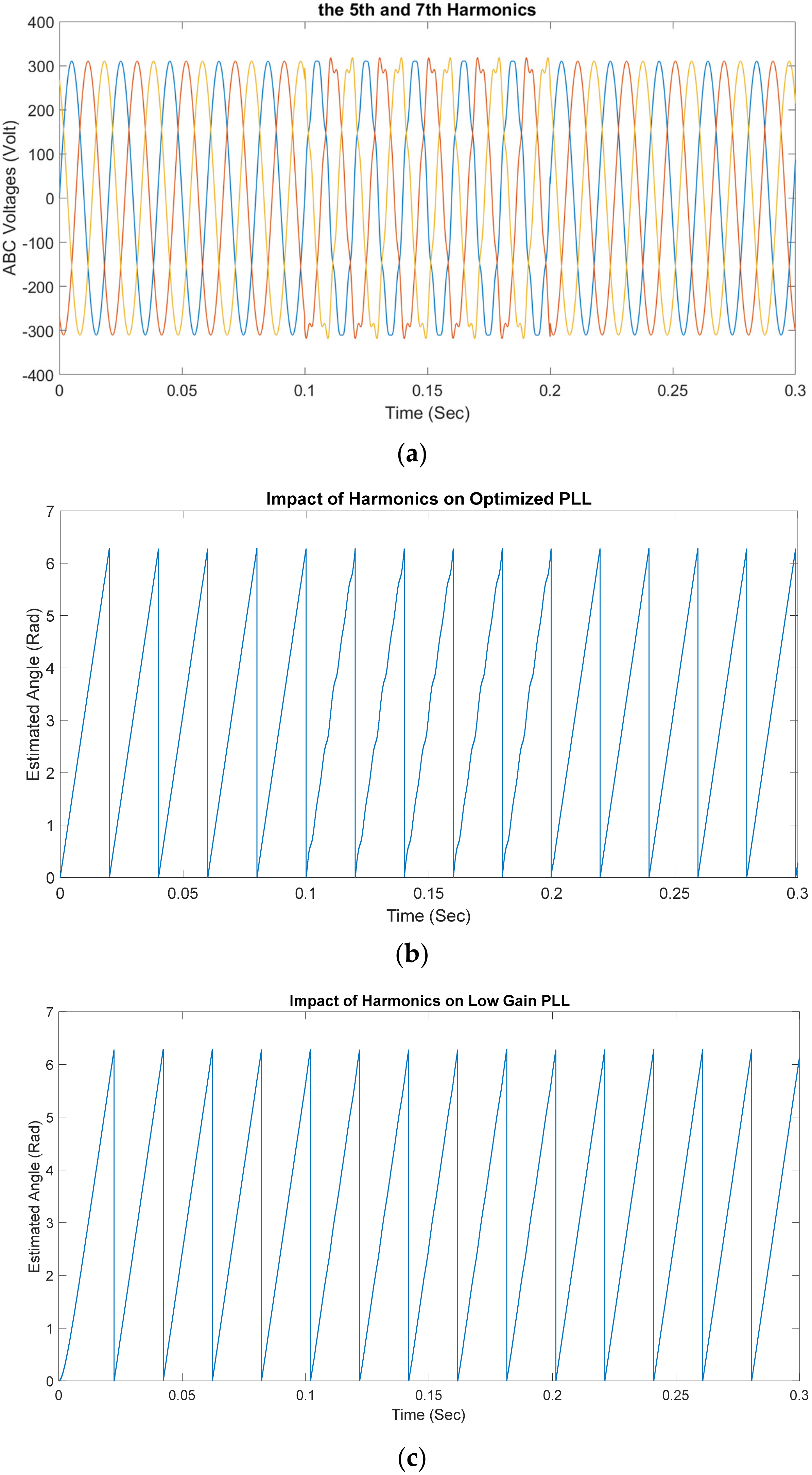
The harmonics impact on the phase estimation test are also conducted by adding the fifth and the seventh harmonics, with magnitudes of 0.05 pu, to the grid’s voltage between 0.1 and 0.2 s, as shown in Figure 12a.
The wide spectrum of frequencies allowed to pass through a high-gain, phase-locked loop such as the one proposed here makes it a bit difficult to maintain accuracy, as shown in Figure 12b. In contrast, the low-gain SRF-PLL shown in Figure 12c is more durable due to harmonics filtration, but the harmonics’ impact over the high-gain PLL is minor compared to the distortion in the phase estimation of low-gain PLLs under voltage sags. The desired design outcome, as stated earlier, tends to focus on LVRT capabilities, which necessitates quick tracking during voltage sags, favoring a high-gain PLL over a low gain; in this case, it is a fair trade-off that serves the design aim.
3.2. Reactive Power Management Simulations and Discussions
The following variable irradiance input signal depicted in Figure 13 is used as the irradiance input of the PV array in all the cases of power injection. The consistency of using the same irradiance input profile is necessary to emphasize the response behavior of the proposed system under different conditions.
3.2.1. First Case (Normal Operating Condition)
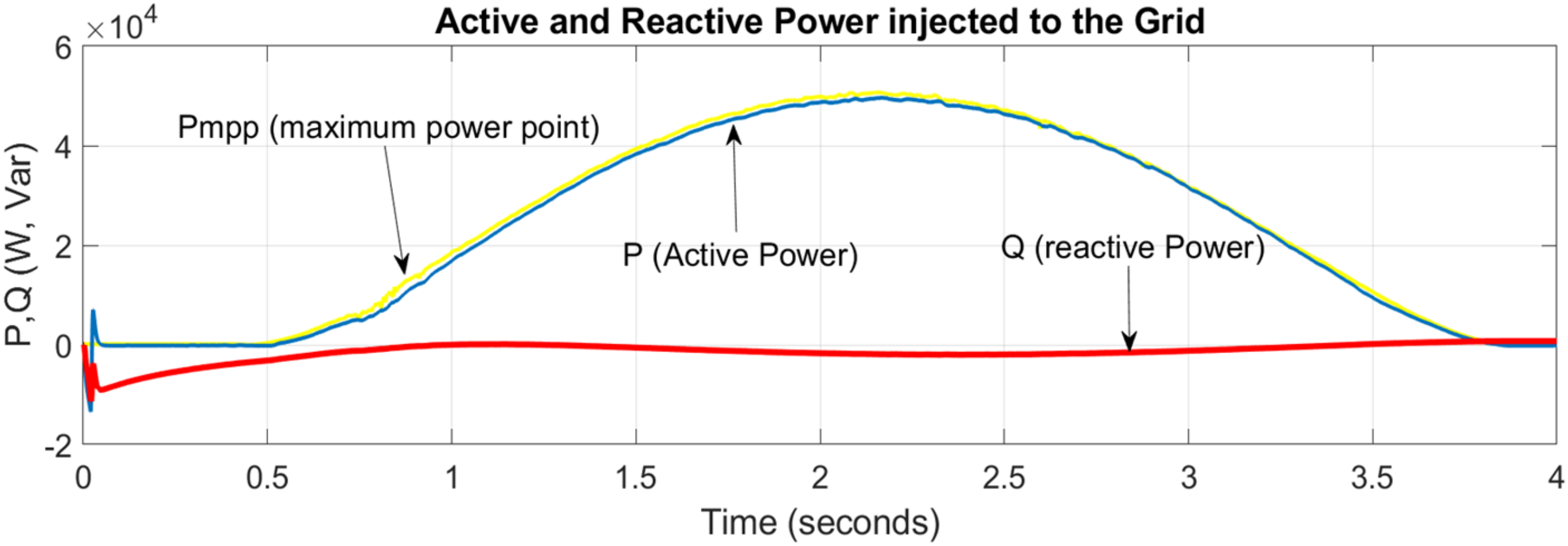
Under normal conditions, the PV system is required to send current in phase with the grid’s voltage to only allow active power injection into the grid; this is achieved through the current’s control loops with linear proportional integral controllers (PIs) in the dq0 reference frame, which is a well-tested method in the literature [2]. The corresponding reference values of direct and quadrant currents are generated through the power management unit. Consequently, the system only injects active power due to the absence of any ancillary service requests, as depicted in Figure 14.
In this case, the PV system acts as a pure active power source and injects the maximum active power extracted by the PV array with the help of its MPPT algorithm, while no reactive power is injected here:
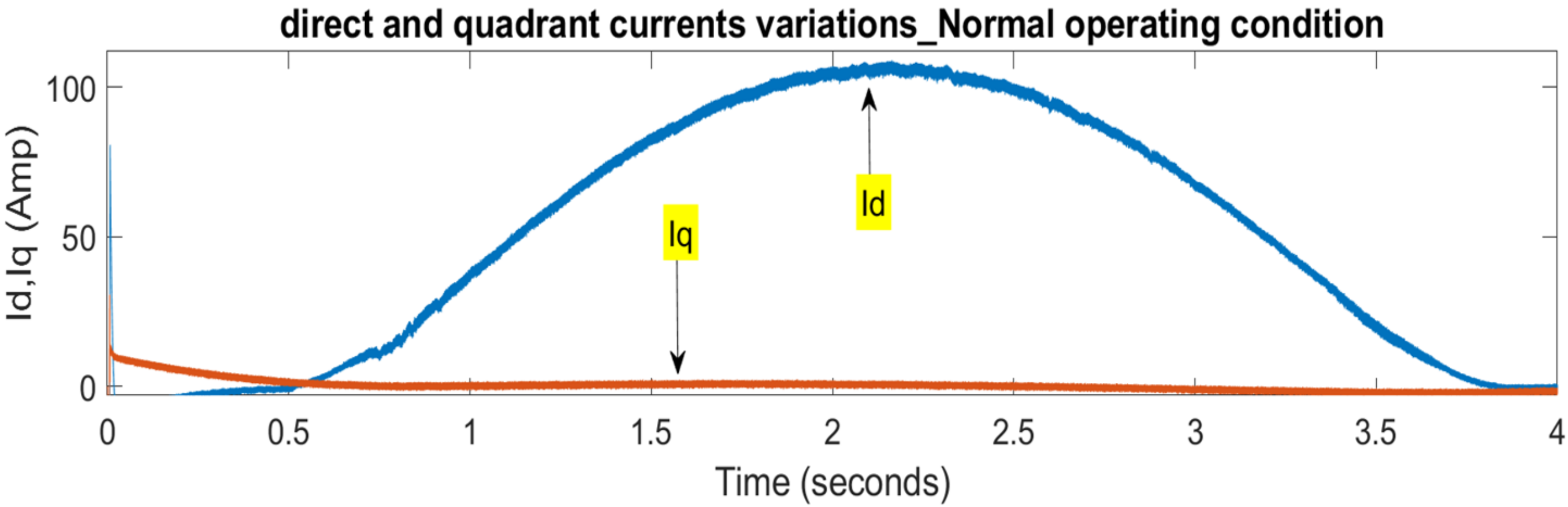
The direct and quadrant currents’ variations under normal operating condition are depicted in Figure 15, and the current control loops are satisfied.
3.2.2. Second Case (MPPT Enabled with Partially Served Intervention)
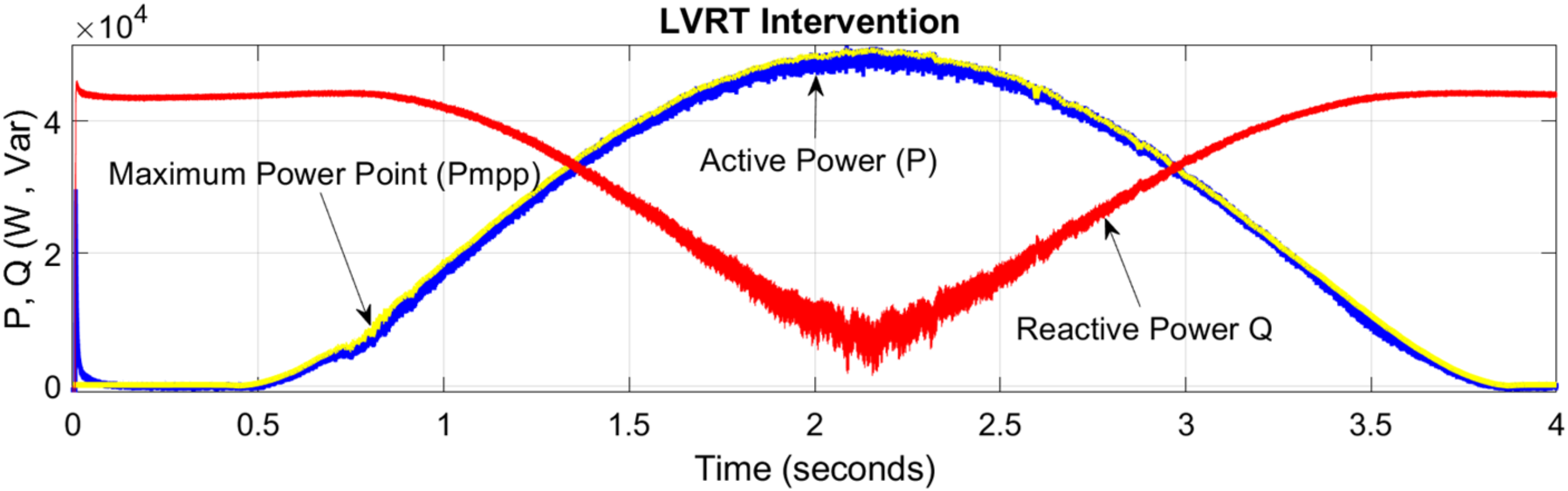
In this case, the system’s response to an ancillary request to support the grid during a fault ride is investigated. In contrast to some of the common methods used in [2,14], where the MPPT state is disabled to inject required reactive power, the proposed power algorithm prioritizes active power over reactive power injection and maintains its MPPT state. As a result, the system provides the maximum possible intervention and the maximum active power, which is depicted in Figure 16.
As shown in Figure 16, the reactive power intervention is at its highest value when the PV inverter has excess current due to low irradiance. However, as the irradiance level increases, PV inverter starts to approach its maximum rated current, and hence, starts lowering the available quadrant current, which results in lowering the injected reactive power to preserve the MPPT state. The active power profile achieved is similar to that of pure active power injection that is presented in Figure 14.
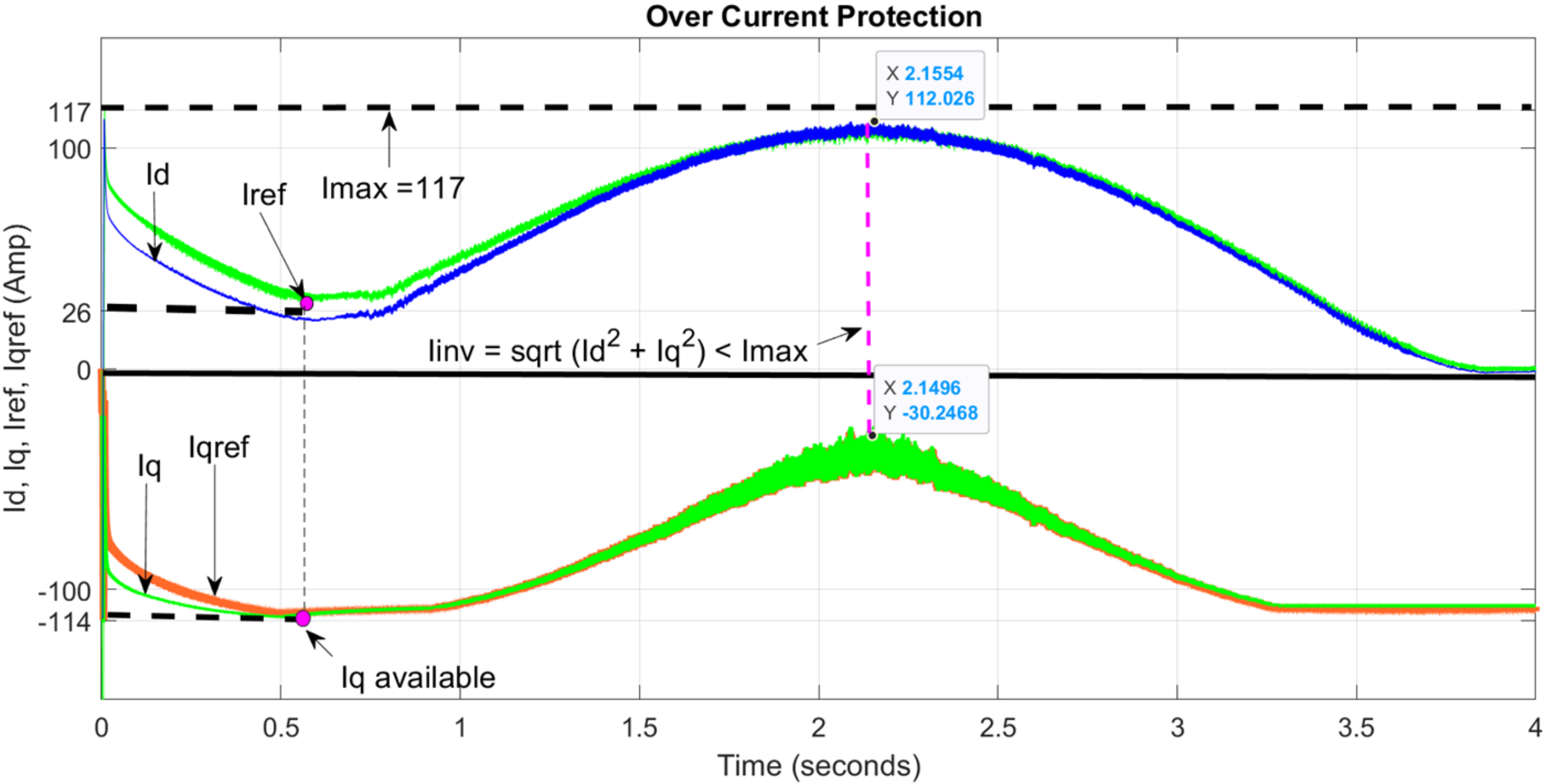
The PV system operates as designed and delivers its nominal capabilities. The proposed power algorithm manages to keep the inverter’s total current under its rated value; this is obtained by constantly calculating the real-time value of the inverter’s current through its components in the dq frame and comparing it to that of the maximum rated value. Specifically, the term in (37) should always be applicable under all operational conditions:
where represents the rated current of the PV inverter, assumed to be 117 A in all calculations.
Figure 17 illustrates the variations of as they are tracking their reference values, and , which are generated by the power algorithm:
Between (0 to 0.5) s, the required current to charge DC bus capacitor is drawn from the grid. From 0.5 s onwards, DC bus is sufficiently charged by the PV array current, which represents an MPPT state. The required current to fulfil the intervention ( is higher than the available marginal quadrant current (, accordingly, as per Equations (29)–(32).
The available quadrant current is a function of the direct current, which represents an ongoing MPPT state; therefore, its value varies according to the variation in irradiance, as observed in Figure 17.
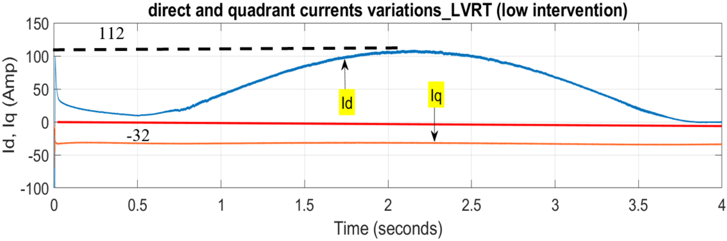
3.2.3. Third Case (MPPT Enabled with Fully Served Intervention)
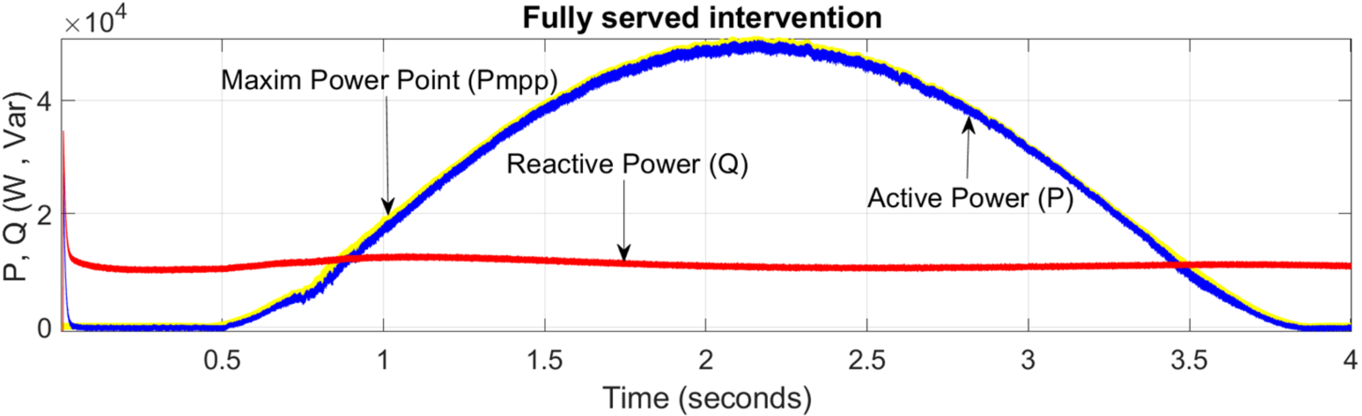
This case features fully served intervention as the required reactive power does not exceed the marginal available current at any point, as depicted in Figure 18.
The intervention is consistent throughout the event. MPPT is enabled by default, which results in fully active and reactive power injection. The direct and quadrant currents variations under this LVRT are depicted in Figure 19.
The rated current of PV inverter is assumed to be 117 A in all calculations; is the direct current when the PV system is operating at its rated power, which is 112 A, and the required quadrant current is calculated as the following:
= 32 A. This is the absolute value of the required quadrant current; therefore, the minimum available quadrant current is:
As the required quadrant current to perform the necessary intervention is less than the marginal available current, the injected quadrant current can be defined as follows:
A, as depicted in Figure 19.
The inverter’s current never reaches its maximum current () at any point. As a result, both the reactive power intervention and the MPPT state are fully served without any interruption.
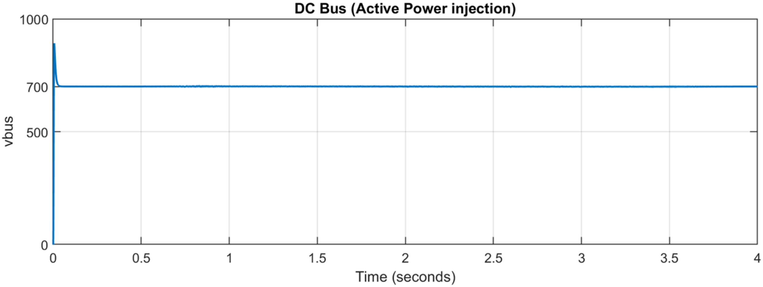
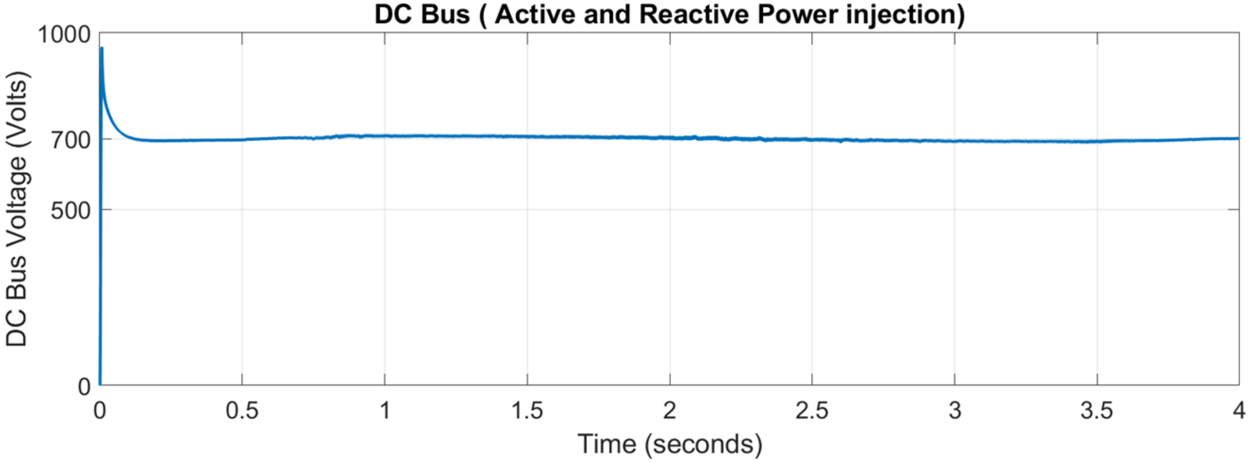
3.3. DC Bus Voltage Stability Simulations and Discussions
Simulations of the DC bus voltage status during normal and LVRT conditions are shown in Figure 20 and Figure 21. The stability of the DC bus is crucial, as the variation of such a parameter has an impact on the inner current control loops’ regulations; higher values might lead to the system shutting down, while a dramatic drop in the voltage will affect the quality of the inverter’s output signals, voltage and current, implicitly [2]. Many control techniques were used in the specific literature to regulate the DC bus voltage such as feedback linearization (FBL) in [18] and the variable DC bus reference for normal and faulty operational modes in [12]. In this paper, the DC bus voltage is regulated using a linear proportional integral (PI) controller with a fixed reference value. The output signal of this voltage control loop is used as the reference value of the direct current to ensure a continuous MPPT state. No fluctuation in the DC bus voltage is observed under normal and reactive power compensation. The proper tuning of the DC voltage regulation loop helps in stabilizing the voltage across the DC bus capacitor. The reference voltage of the DC bus is fixed at (700 volts), which falls under the allowed range of three phase topologies between 600 and 1000 volts [28].
4. Conclusions
The usefulness of an optimized high-gain SRF-PLL during a voltage disturbance was investigated and confirmed via Simulink simulations. The performance under voltage sags was far more resilient and accurate under voltage disturbances in comparison with a conventional phase-locked loop. A novel reactive power management algorithm was proposed to give the PV system a low-voltage ride through the LVRT capability without the need to disable its MPPT state and without scarifying the PV inverter safety. The system performance was verified under the variant irradiance input profile and under two different operating conditions. The first was when only active power is allowed to be injected, and the second is when reactive power injection is requested. The graphical results were presented in context to verify the claimed theoretical capabilities of the system. The system managed to perform reactive power injection without exceeding the inverter’s rated current due to its implemented overcurrent protection feature. The MPPT state was enabled under normal and LVRT conditions; the system managed to preserve the maximum power point state while simultaneously participating in the ancillary services. The system’s contribution to the power quality enhancement measures will make the DG system more financially viable; however, the financial feasibility of the genetic algorithm and the reactive power management implementation was not discussed here, but it is worth considering in future work.
Author Contributions
Conceptualization, B.A., M.N. and E.R.; methodology, B.A., M.N. and E.R.; software, B.A.; validation, M.N., E.A. and E.R.; formal analysis, B.A. and M.N.; investigation, B.A.; resources, B.A. and M.N.; data curation, B.A.; writing—original draft preparation, B.A.; writing—review and editing, B.A., M.N. and E.A.; visualization, E.A.; supervision, M.N. and E.R.; project administration, M.N.; funding acquisition, E.R. and M.N. All authors have read and agreed to the published version of the manuscript.
Funding
This research received no external funding.
Conflicts of Interest
The authors declare no conflict of interest.
References
- Naderi, Y.; Hosseini, S.H.; Zadeh, S.G.; Mohammadi-Ivatloo, B.; Vasquez, J.C.; Guerrero, J. An overview of power quality enhancement techniques applied to distributed generation in electrical distribution networks. Renew. Sustain. Energy Rev. 2018, 93, 201–214. [Google Scholar] [CrossRef] [Green Version]
- Muhammad, T.; Raihan, S.R.S.; Abd Rahim, N. PV inverter with decoupled active and reactive power control to mitigate grid faults. Renew. Energy 2020, 162, 877–892. [Google Scholar]
- Gielen, D.; Gorini, R.; Wagner, N.; Leme, R.; Gutierrez, L.; Prakash, G.; Janeiro, L.; Vale, G.; Feng, J.; Renner, M.; et al. Global Energy Transformation: A Roadmap to 2050; IRENA: Abu Dhabi, United Arab Emirates, 2018. [Google Scholar]
- Stetz, T.; Martenl, F.; Braun, M. Improved Low Voltage Grid-Integration of Photovoltaic Systems in Germany. IEEE Trans. Sustain. Energy 2013, 4, 534–542. [Google Scholar] [CrossRef]
- Safayet, A.; Fajril, P.; Husain, I. Reactive Power Management for Overvoltage Prevention at High PV Penetration in a Low-Voltage Distribution System. IEEE Trans. Ind. Appl. 2017, 53, 5786–5794. [Google Scholar] [CrossRef]
- Seong, U.-S.; Hwang, S.-H. Analysis of Phase Error Effects Due to Grid Frequency Variation of SRF-PLL Based on APF. J. Power Electron. 2016, 16, 18–26. [Google Scholar] [CrossRef] [Green Version]
- Kulkarni, A.; John, V. Design of synchronous reference frame phase-locked loop with the presence of dc offsets in the input voltage. IET Power Electron. 2015, 8, 2435–2443. [Google Scholar] [CrossRef] [Green Version]
- Nicolini, A.; Pinheiro, H.; Carnielutti, F.; Massing, J. PLL parameters tuning guidelines to increase stability margins in multiple three-phase converters connected to weak grids. IET Renew. Power Gener. 2020, 14, 2232–2244. [Google Scholar] [CrossRef]
- Radwan, E.; Salih, K.; Awada, E.; Nour, M. Modified phase locked loop for grid connected single phase inverter. Int. J. Electr. Comput. Eng. 2019, 9, 3934–3943. [Google Scholar] [CrossRef]
- Yang, Y.; Blaabjerg, F. Low-Voltage Ride-Through Capability of a Single-Stage Single-Phase Photovoltaic System Connected to the Low-Voltage Grid. Int. J. Photoenergy 2013, 2013, 257487. [Google Scholar] [CrossRef] [Green Version]
- Ranjan, A.; Kewat, S.; Singh, B. DSOGI-PLL With In-Loop Filter Based Solar Grid Interfaced System for Alleviating Power Quality Problems. IEEE Trans. Ind. Appl. 2021, 57, 730–740. [Google Scholar] [CrossRef]
- George, C.K.; Qing-Chang, Z.; Wen-Long, M. PLL-less Nonlinear Current-limiting Controller for PLL-less Nonlinear Current-limiting Controller for Analysis and Operation Under Grid Faults. IEEE Trans. Ind. Electron. 2016, 63, 5582–5591. [Google Scholar]
- Merabet, A.; Labib, L.; Ghias, A.M.Y.M.; Ghenai, C.; Salameh, T. Robust Feedback Linearizing Control with Sliding Mode Compensation for a Grid-Connected Photovoltaic Inverter System Under Unbalanced Grid Voltages. IEEE J. Photovolt. 2017, 7, 828–838. [Google Scholar] [CrossRef]
- Hamrouni, N.; Younsi, S.; Jraidi, M. Flexible active and reactive power control strategy of a LV grid connecetd PV system. Energy Proc. 2019, 162, 325–338. [Google Scholar] [CrossRef]
- Li, X.; Zhang, H.; Shadmand, M.B. Model Predictive Control of a Voltage-Source Inverter with Seamless Transition between Islanded and Grid-Connected Operations. IEEE Trans. Ind. Electron. 2017, 64, 7906–7918. [Google Scholar] [CrossRef]
- Sajadian, S.; Ahmadi, R. ZSI for PV systems with LVRT capability. IET Renew. Power Gener. 2018, 12, 1286–1294. [Google Scholar] [CrossRef]
- Bighash, E.Z.; Sadeghzadeh, S.M.; Ebrahimzadeh, E.; Blaabjerg, F. Improving performance of LVRT capability in single-phase grid-tied PV inverters by a model-predictive controller. Int. J. Electr. Power Energy Syst. 2018, 98, 176–188. [Google Scholar] [CrossRef]
- Mishra, M.K.; Lal, V.N. An improved methodology for reactive power management in grid integrated solar PV system with maximum power point condition. Sol. Energy 2020, 199, 230–245. [Google Scholar] [CrossRef]
- Marks, N.D.; Summers, T.J.; Betz, R.E. Photovoltaic power systems: A review of topologies, converters and controls. In Proceedings of the 2012 22nd Australasian Universities Power Engineering Conference (AUPEC), Bali, Indonesia, 26–29 September 2012. [Google Scholar]
- Mohammad, R.M.L.; Wijaya, F.D. High Performance Multistring Converter Topology for Three-Phase Grid Tied 200 kW Photovoltaic Generating System. IJITEE Int. J. Inf. Technol. Electr. Eng. 2017, 1, 51–62. [Google Scholar] [CrossRef] [Green Version]
- Chung, S.-K. Phase-locked loop for grid-connected three-phase power conversion systems. IEE Proc. Electr. Power Appl. 2000, 147, 213–219. [Google Scholar] [CrossRef]
- Best, R.E. Phase Locked Loops, Design, Simulation and Applications, 6th ed.; McGraw-Hill: New York, NY, USA, 2004. [Google Scholar]
- Freijedo, F.D.; Doval-Gandoy, J.; Lopez, O.; Acha, E. Tuning of Phase-Locked Loops for Power Converters Under Distorted Utility Conditions. IEEE Trans. Ind. Appl. 2009, 45, 2039–2047. [Google Scholar] [CrossRef]
- Karimi-Ghartemani, M. Enhanced Phase-Locked Loop Structures for Power and Energy Applications; John Wiley & Sons: Hoboken, NJ, USA, 2014. [Google Scholar] [CrossRef]
- Meersman, B.; De Kooning, J.; Vandoorn, T.; Degroote, L.; Renders, B.; Vandevelde, L. Overview of PLL methods for Distributed Generation units. In Proceedings of the 45th International Universities Power Engineering Conference, UPEC2010, Cardiff, UK, 31 August–3 September 2010. [Google Scholar]
- AbdelRassoul, R.; Ali, Y.; Saad, M. Genetic Algorithm-Optimized PID Controller for better Performance of PV System. Commun. Appl. Electron. 2016, 5, 55–60. [Google Scholar] [CrossRef]
- Jayachitra, A.; Vinodha, R. Genetic Algorithm Based PID Controller Tuning Approach for Continuous Stirred Tank Reactor. Adv. Artif. Intell. 2014, 2014, 791230. [Google Scholar] [CrossRef]
- Teodorescu, R.; Liserre, M.; Rodríguez, P. Chapter 10: Control of grid converters under grid faults. In Grid Converters for Photovoltaic and Wind Power Systems, 1st ed.; Wiley and Sons Publications: Chichester, UK, 2011; Volume 1, pp. 237–289. [Google Scholar]
- Lin, F.-J.; Lu, K.-C.; Ke, T.-H.; Yang, B.-H.; Chang, Y.-R. Reactive Power Control of Three-Phase Grid-Connected PV System During Grid Faults Using Takagi–Sugeno–Kang Probabilistic Fuzzy Neural Network Control. IEEE Trans. Ind. Electron. 2015, 62, 5516–5528. [Google Scholar] [CrossRef]
- Kathiresan, A.; PandiaRajan, J.; Sivaprakash, A.; Babu, T.S.; Islam, R. An Adaptive Feed-Forward Phase Locked Loop for Grid Synchronization of Renewable Energy Systems under Wide Frequency Deviations. Sustainability 2020, 12, 7048. [Google Scholar] [CrossRef]
- Sevilmiş, F.; Karaca, H. Performance analysis of SRF-PLL and DDSRF-PLL algorithms for grid interactive inverters. Int. Adv. Res. Eng. J. 2019, 3, 116–122. [Google Scholar] [CrossRef] [Green Version]
Figure 1.
Two-stage grid-connected PV system’s control scheme including the added power management unit and GA algorithm.
Figure 1.
Two-stage grid-connected PV system’s control scheme including the added power management unit and GA algorithm.

Figure 2.
Block diagram of the synchronous reference-frame-based PLL.

Figure 3.
Flow diagram of the genetic algorithm used to optimize SRF-PLL.

Figure 4.
PLL step responses: (a) non-optimized step response, (b) different step responses generated by GA, (c) optimized step response.
Figure 4.
PLL step responses: (a) non-optimized step response, (b) different step responses generated by GA, (c) optimized step response.

Figure 5.
Different transfer functions Bode diagrams generated by the genetic algorithm during optimization process.
Figure 5.
Different transfer functions Bode diagrams generated by the genetic algorithm during optimization process.

Figure 6.
DC bus voltage control loop with reference value of 700.

Figure 7.
Electrical circuit of the PV inverter connection with the grid.

Figure 8.
Currents control loops.

Figure 9.
Flowchart of reactive power management algorithm.

Figure 10.
Trigonometric relation between Imax , and available.

Figure 11.
Voltage sags impact on PLL, (a) voltage sags of 50%, (b) impact on optimized SRF-PLL, (c) impact on low-gain PLL.
Figure 11.
Voltage sags impact on PLL, (a) voltage sags of 50%, (b) impact on optimized SRF-PLL, (c) impact on low-gain PLL.

Figure 12.
Harmonics impact on PLL, (a) 5th and 7th harmonics of 0.05 pu, (b) impact on optimized SRF-PLL, (c) impact on low-gain PLL.
Figure 12.
Harmonics impact on PLL, (a) 5th and 7th harmonics of 0.05 pu, (b) impact on optimized SRF-PLL, (c) impact on low-gain PLL.

Figure 13.
PV array irradiance input profile.

Figure 14.
Power injection under normal condition (P = Pmpp, Q = 0).

Figure 15.
Id and Iq variations under normal condition (P = Pmpp, Q = 0).

Figure 16.
Maximum possible intervention under LVRT and high requirements of reactive power injection (P = Pmpp, Qreq = 55 K Var).
Figure 16.
Maximum possible intervention under LVRT and high requirements of reactive power injection (P = Pmpp, Qreq = 55 K Var).

Figure 17.
Overcurrent protection feature, (P = Pmpp, Qreq = 55 K Var).

Figure 18.
Fully served intervention (P = Pmpp, Qreq = 15 K Var).

Figure 19.
Id and Iq variation under LVRT (P = Pmpp, Qreq = 15 K Var).

Figure 20.
DC bus voltage state under normal condition (P = Pmpp, Q = 0).

Figure 21.
DC bus voltage state under reactive power compensation (P = Pmpp, Q ≠ 0).


Table 1.
GA optimization criterions.
| Criterion | Considered Range/Value | Obtained by | Converged at |
|---|---|---|---|
| Voltage magnitude (volts) | 310.3 | _ | _ |
| Corner frequency (r/s) | 314 to 9400 | Bounding Ki | ≈6400 |
| Damping ratio Settling Time (s) | 0.7 to 1 Minima | Const fun Cost fun | 0.93 1.2 m. s |
Publisher’s Note: MDPI stays neutral with regard to jurisdictional claims in published maps and institutional affiliations. |
© 2022 by the authors. Licensee MDPI, Basel, Switzerland. This article is an open access article distributed under the terms and conditions of the Creative Commons Attribution (CC BY) license (https://creativecommons.org/licenses/by/4.0/).
Share and Cite
MDPI and ACS Style
Aldbaiat, B.; Nour, M.; Radwan, E.; Awada, E. Grid-Connected PV System with Reactive Power Management and an Optimized SRF-PLL Using Genetic Algorithm. Energies 2022, 15, 2177. https://0-doi-org.brum.beds.ac.uk/10.3390/en15062177
AMA Style
Aldbaiat B, Nour M, Radwan E, Awada E. Grid-Connected PV System with Reactive Power Management and an Optimized SRF-PLL Using Genetic Algorithm. Energies. 2022; 15(6):2177. https://0-doi-org.brum.beds.ac.uk/10.3390/en15062177
Chicago/Turabian StyleAldbaiat, Bashar, Mutasim Nour, Eyad Radwan, and Emad Awada. 2022. "Grid-Connected PV System with Reactive Power Management and an Optimized SRF-PLL Using Genetic Algorithm" Energies 15, no. 6: 2177. https://0-doi-org.brum.beds.ac.uk/10.3390/en15062177
Note that from the first issue of 2016, this journal uses article numbers instead of page numbers. See further details here.