1. Introduction
The transition from fossil fuels to green energy is facilitated by the current technological advancements, which increase the efficiency of clean generators, favoring their large-scale diffusion [
1].
Power systems, traditionally built to handle passive and controllable loads, are now put to the test by variable power generators, such as wind, whose profile prediction is still challenging. A large amount of renewable energy generation can lead to high transmitted powers on the lines, causing them to operate near or beyond established loadability margins. Therefore, it is necessary to revise traditional power line operational policies to maintain optimal line management. Transmission lines are characterized by thermal limits expressing their maximum operating temperature. The thermal limits directly affect the load of such lines, playing a crucial role in determining the maximum current intensity of the conductor.
Static Line Rating (SLR) aims at computing the maximum current capacity of the conductor, providing a single, fixed value representative of the worst-case scenario. This leads to conservative operation conditions of the lines, limiting the full employment of line capacity over time.
Differently, dynamic thermal line rating (DTLR) introduces the possibility of adapting the capacity of the transmission line dynamically. The significant advantages of DTLR over SLR include a possible reduction in line congestion caused by the static thermal limit, as well as easier integration of renewable energy sources. The Transmission System Operator (TSO) can adapt the current capacity based on the impact of the current atmospheric condition on the conductor temperature.
Nevertheless, the temperature could vary along bare overhead lines, yielding the necessity of repeating the temperature estimation for several points of the lines. This is particularly relevant when the line covers weather-varying distances of dozens of kilometers. The most relevant temperature among these repeated measurements is the highest, closest to the conductor thermal limit. The necessity of repeated measures significantly increases the costs of sensors, labor, and maintenance.
DTLR is an essential topic in power systems where the research community has produced many contributions. In this review, the DTLR was analyzed by grouping the manuscripts according to existing methods to perform DTLR. Mainly, DTLR includes many tasks such as: (i) estimation of the load capability curve given the current weather conditions, (ii) monitoring of the temperature conductor over the line, (iii) short-term forecasting of conductor temperature to assess transient emergency rating, which is currently an ongoing area of research [
2]. Existing approaches for conductor temperature estimation belong to two main categories:
Direct methods are characterized by the measurement, through sensors, of the conductor temperature or typical characteristics related to it, such as sag, voltage, ground clearance, and mechanical stress [
3]. The temperature measurement is often obtained employing expensive devices applied to a single point of the line [
4], to measure the conductor surface temperature, which may differ from its core temperature. A typical direct method is the adoption of the Power Donut™ sensor to monitor the conductor temperature, current, and vibration in a single point of the line [
3]. They are considered expensive [
5] and measure surface temperature.
Indirect methods estimate the conductor temperature without actual measurement. For example, some applications estimate the average line conductor temperature from the Phasor measurement units using line parameters estimation [
6]. Differently, the approaches estimating the point line conductor usually rely on real-time measurements of atmospheric conditions [
7,
8] around the conductor, such as air temperature and sun irradiance, and estimate the conductor temperature by solving an energy balance equation. A widely employed indirect method for estimating the conductor temperature of bare overhead lines given the weather conditions is provided by the IEEE 738 standard [
9], presented in
Section 2.1.
Since the IEEE 738 indirect approach may fail because of sensor measurements errors, recent research focused on alternative methods. For instance, Refs. [
10,
11] proposed a Recurrent Neural Network using only temperature and line current. Unfortunately, these approaches have two main limitations: first, they still need the conductor temperature sensor; second, they neglect the weather condition, which may considerably affect the line conductor.
Reference [
12] proposes the adoption of Multi-Layer-Perceptron Network to map the relationship between historical samples of conductor and ambient temperature as inputs and convection cooling factor and conductor heat capacitance as outputs, followed by a Parameter Estimation Tester (PET) that maps the network outputs to the conductor temperature and its derivative. However, the IEEE 738 standard is used to prepare the training data, therefore the mapping suffers from sudden changes of input parameters, such as the sun irradiance, which is shown to be a frequent reason for IEEE 738 critical errors (
Section 4.3). Furthermore, the experimental comparison is made with the IEEE 738 estimation, therefore not reflecting the ability of the model to follow the real conductor temperature.
Authors in [
10] use an Echo State Network (ESN), a novel recurrent neural network (RNN), to learn the non-linear overhead conductor thermal dynamics, and their results show an encouraging match between the ESN and the IEEE 738 model under similar weather conditions. Nevertheless, the match with IEEE 738 does not necessarily mean that the model can follow the actual conductor temperature since both could be inaccurate.
Recent works focus on the security aspect of dynamic thermal rating by proposing specific deep learning architecture with customized cost functions to consider the DTLR security based on the required probability of exceedance [
13], as well as DTLR variations improved with current ratio of negative and positive sequences, and voltage criterion for successfully differentiating between faults and unsafe and safe overloading [
14].
Finally, the adoption of machine learning techniques has emerged as a key driver for the development of Industry 4.0. Relevant results include the exploitation of sensors data for analysis, monitoring, and security purposes [
15], as well as energy management for smart buildings [
16].
With these premises and at the best of the authors’ knowledge, it seems that state-of-the-art approaches do not address the most crucial issues: (i) to estimate the conductor temperature without the deployment of a temperature sensor, whose installation and maintenance require interrupting the line operation, and (ii) compensate for diverging temperature estimation over time, which usually affects methods that do not use the actual temperature but rely on the IEEE 738 standard for the training data.
For this reason, the TSOs are interested in deploying a limited number of sensors (only for the weather conditions and accessible without interrupting the line operation) and in the development of low-computational burden models, which can be processed by local-processing units in a network of cooperative sensors.
The advantage of this manuscript is the adoption of real, measured conductor temperature for the mapping, which, therefore, shows a reduction in sensitivity to sudden changes of the input parameters typical of the IEEE 738 standard using machine learning methodologies, which are suitable for the architecture described above.
1.1. Digital Twin
A digital twin (DT) is a virtual model of a physical system characterized by seamless integration between the cyber and physical spaces [
17]. Seamless integration is achieved by integrating the physical and virtual data within the DTs [
18]. DT approaches are becoming more and more pervasive in different power system research areas: Power Grid Online Analysis [
19], where a DT can mirror a large scale power grid in real-time with only a sub-second delay; substations virtualization [
20] where a “dynamic connection, two-way transmission” relationship is established between a substation and its DT; DT are receiving increasing attention also from the industrial side: patents have been granted for a system to monitor the state of turbines of a wind farm [
21] and for a DT-based cooling process of a power system [
22]. However, in the context of DTLR, the notion of DT appears, to the best of the authors’ knowledge, to be still novel.
Machine learning (ML) is often at the core of DT implementations [
23,
24] because of its capacity to extract meaningful relations from data. Once trained, a ML model can act as an equivalent of a physical system: given a specific input, it produces a corresponding output that ideally coincides with the physical system output. In this sense, a DT can adopt ML to model reality; and a standard ML model can be the enabler of the DT.
A further significant difference lies in the connection with the physical world: while the ML model does not have to interact with the modeled object, a DT does. Its integration with reality is bi-directional and automatic: any change in the physical world is reflected in the DT, and the enhanced decision-making outcomes of the latter are applied to the former. A DT also differs from a traditional physics-based simulation model. Although the latter is generally defined by closed-form mathematical formulations with well-defined hypotheses, a DT often has a non-parametric, data-driven approach (often based on a sensor network).
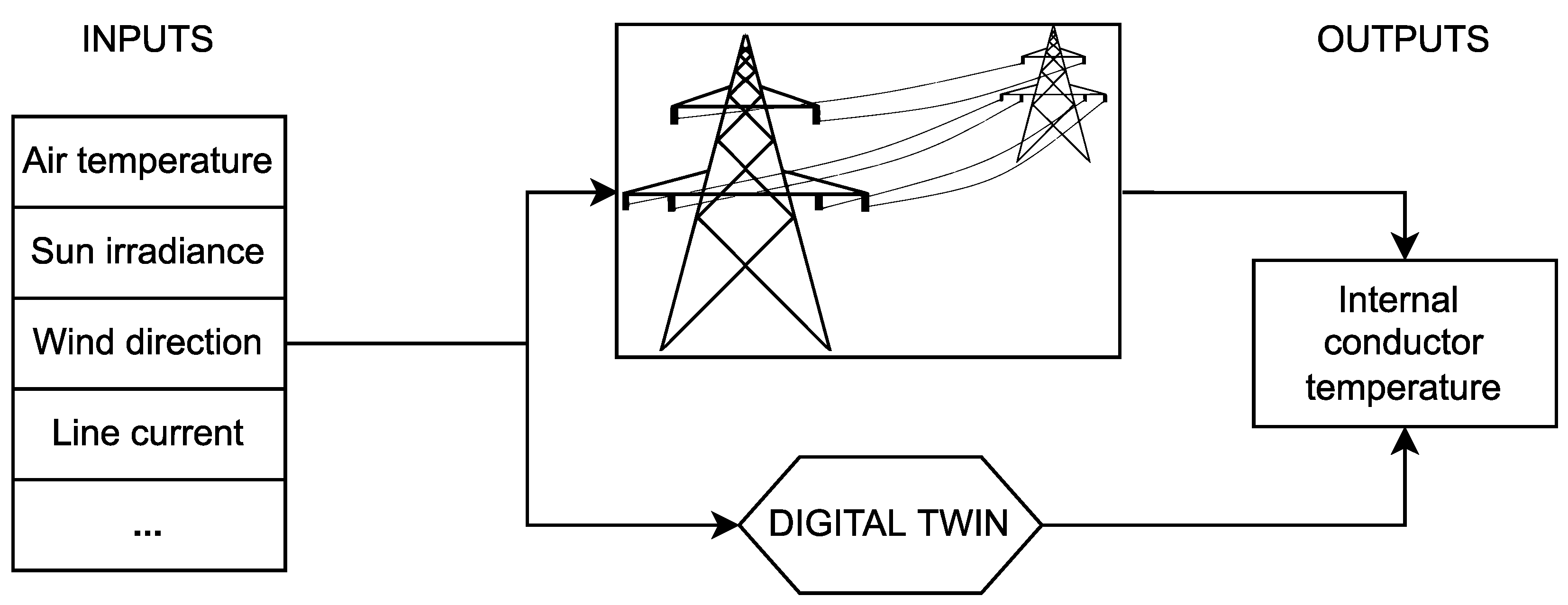
This manuscript recommends adopting a DT approach for dynamic thermal line rating by showing the performances of the ML models that would be at the core of a corresponding DT architecture. The complete DT architecture, including a simulation interface, a connection with the physical space, and a control mechanism to employ the mentioned ML models, is left for future research. For the sake of simplicity, in the following, the term Digital Twin will refer to the ML models adopted. A high level graphical representation of the proposed approach is shown in
Figure 1.
1.2. Authors’ Contribution
The main contributions of this paper are:
The proposal of a Digital Twin approach for DTLR based on Machine Learning (ML): by employing a conductor temperature sensor to collect measurements on the line of interest for a limited amount of time, the DT would be trained using a ML model on the measured data. After the training phase, the DT will act as a complete virtual equivalent of the physical system modeled by the IEEE 738 standard;
A dimensionality reduction study: as shown in
Section 4.2, the proposed approach could suggest which sensors measurements have a significant role in the sensors-temperature mapping through
feature selection [
25], providing the TSO with meaningful information in terms of sensors’ importance;
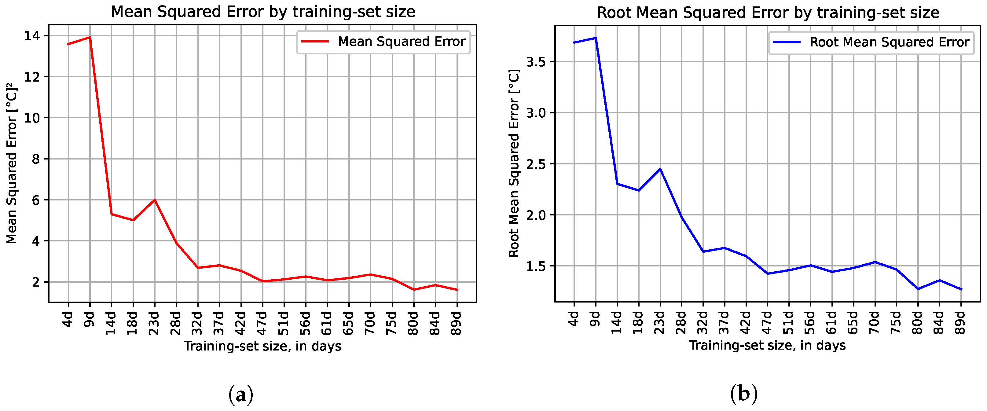
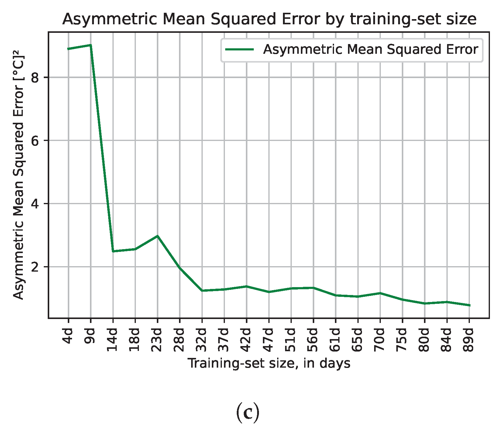
An investigation about the training phase duration: the DT can be trained with different amounts of historical data points, and the collected performances suggest a minimum duration of the training phase. This is the recommended minimal utilization time of the mentioned temperature sensor;
A prediction error analysis: the knowledge of the actual measured temperature allows the study of the areas of severe over/under-estimation by the IEEE-738 standard, utilizing a correlational and graphical analysis, presented in
Section 4.3.
The experimental assessment presented in
Section 4, shows that relying on a DT approach can significantly improve the accuracy of the estimated temperature with respect to the IEEE 738 standard: the prediction could influence the physical system based by adapting the current load, leading to better optimization of the bare overhead line.
2. Mathematical Formalization
A set of data and , respectively the matrix of acquired weather and measured line current data; and the vector of measured conductor temperature, is given. M is the number of total samples, and S is the number of acquired variables. Preliminary, the data above can be split into training and validation sets. Let, and , , , where . , where , is the reduced input data matrix, which contains only the non-constant variables for the prediction. indicates the vector of the estimated conductor temperature, which can also be split in training and validation set, and , respectively.
This section provides a formal description of the methodologies adopted in the manuscript. First,
Section 2.1 describes the IEEE 738 standard, providing the non-steady-state equation used to predict the conductor temperature. Next, sect ion
Section 2.2 introduces the proposed Digital Twin models, namely black-box and grey-box [
26]. Finally,
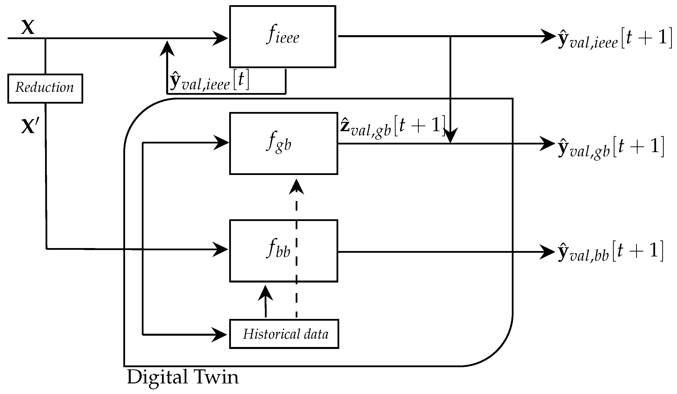
Section 2.3 presents the core algorithm of the proposed Digital Twin approaches: the Random Forest Regressor. A graphical summary is illustrated in
Figure 2.
2.1. IEEE 738 Standard
The IEEE 738 standard was developed in 1986 to “provide a practical, stable, and uniform (calculation) method for use and reference” [
9]. It describes a numerical method for relating the core and surface temperature of a bare overhead electrical conductor to steady or time-varying electrical currents and weather conditions.
The static nature of this model collides with the highly dynamic behavior of the different parameters of the model (electric current and weather conditions, among others). For this reason, the model is run multiple times across short time spans, within which the values of the input parameters can be assumed to be constant.
The change in conductor temperature
over the time interval
is calculated using the non-steady-state heat balance (Equation (
1)). At the end of the time interval, the temperature is simply the sum of the initial temperature and its change. Then, using a series of such time intervals, the conductor temperature at the end of each interval is calculated to approximate the conductor temperature. In summary, the temperature is a time-varying quantity, depending on the current in the line and the weather conditions.
In Equation (
1),
[W/m] is the convection heat loss rate per unit length,
[W/m] is the radiated heat loss rate per unit length,
[J/(m-°C)] is the total heat capacity of conductor,
[°C] is the average conductor temperature,
[W/m] is the heat gain rate from sun,
I [A] is the conductor current,
[
/m] is the AC resistance of conductor at temperature
.
Therefore, a model based on IEEE 738,
, is an iterative model which supplies the prediction at
as follows:
Equation (
2) shows that IEEE 738 does not require any training data since it is just the numerical integration of the first-order differential Equation (
1).
2.2. Proposed DT-Based Models
The proposed black-box model needs training data to perform and predicts the future temperature conductor considering only the weather and line current data.
where
is the vector of predicted conductor temperature by using a black-box model and
is the black-box model. Hence, the black-box model is trained as follows:
where the TRAIN function represents the training phase and returns a trained ML model.
The grey-box model also needs a set of training data to perform, but its aim is to correct the prediction of IEEE 738 model as follows:
where
is vector of the predicted error between the IEEE 738 and the actual temperature conductor, and
is the vector of the grey-box model final output. Particularly, the latter is obtained as:
where
is the grey-box model function, which is trained using the following map in the training step:
where
is the vector of the error between the true conductor temperature value and the estimated temperature of the conductor by IEEE 738 and the TRAIN function represents, as in (
4), the training phase and returns a trained ML model. Particularly, each
n-th element of this vector is linked to the error of the
-th step. Hence, the generic sample of this vector is equal to:
2.3. Learning Algorithm
This work is characterized by the adoption of a Random Forest Regressor learning algorithm [
27] from the scikit-library [
28]. Preliminary experiments showed an outperformance of the considered model with respect to other approaches, such as linear regressor [
29], k-NN [
30], and SVM [
31]. Therefore, in a winner-take-it-all approach, only the top-performing technique in the preliminary experiments has been chosen for the experimental assessment.
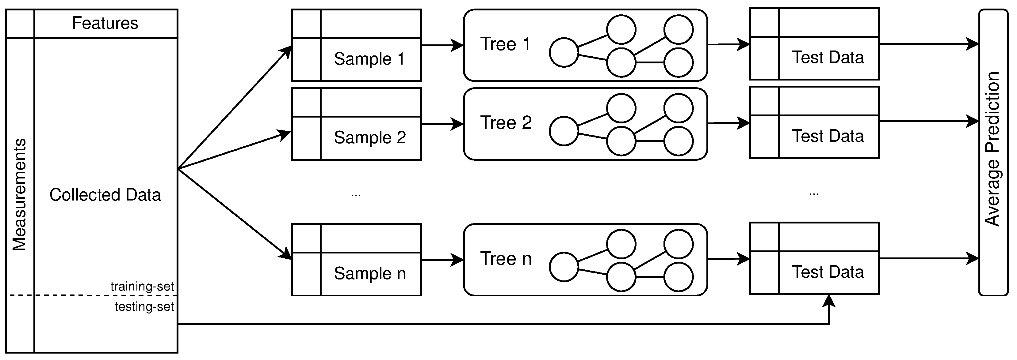
A Random Forest Regressor is a learning algorithm that leverages ensemble learning, combining predictions from multiple decision trees regressors to make a more accurate prediction than a single model. Each decision tree is trained with a different random subsample of the original data, and their final predictions are averaged. A random forest regression can effectively model linear and non-linear relationships in several other domains [
32].
Constant columns in the original dataset do not provide meaningful information for a Random Forest model, therefore the need for the reduced input data matrix presented in
Section 2.2.
Every decision tree is built top-down from a root node, containing all the data points in the corresponding random subsamples of and its construction partitions the data into homogeneous groups by searching the feature value that maximizes a separation criteria.
A flowchart of a Random Forest algorithm with
n trees is presented in
Figure 3: the process starts with the collected data, which are split into training-set and testing-set. Next, the training-set is randomly subsampled
n times, and each sample is used to build a decision tree. Every decision tree is then used to perform prediction on the unseen testing-set: the final Random Forest prediction is the average of each tree prediction.
3. Case Study Description
This section aims to show that adopting a DT can be of significant help in estimating the internal conductor temperature. In particular, storing the physical sensors data allows data-driven approaches to be adopted. A ML model can learn the relationship between the collected measures and the conductor temperature from historical data. Therefore, given more recent sensor measurements, the model can predict unseen values for the temperature.
3.1. Data
This manuscript employs real data gained from a sensor station installed on a tower of a High Voltage (HV) Overhead line (OHL) [
33]. The time resolution is 1 min. The sensor station is installed about 45 m from the ground. It is equipped with a thermopile, which measures the solar radiative flow, an air temperature sensor, with a resolution of 1 °C, and a 3D ultrasonic anemometer, which measures wind speed components with an expected measurement error of
m/s. Since the conductor is placed at a higher height than the sensor station, software estimates wind speed at
m according to wind shear equation [
34], where the friction coefficients are experimentally computed using a neighbor mast station. The data are broadcast in real-time to a server, which couples the latter with the line current measurement for each
t acquired at
, which is returned from the TSO’s Energy Management System (EMS). Since
r is set equal to 60 s, a specific line current and weather variables stable condition are linked to a resulting conductor temperature reached after 60 s from a precise initial conductor temperature. In addition, to validate the performance of both methodologies, a device to measure the conductor temperature is temporarily installed on the conductor, called Micca™. The latter will not be employed in the final operative configuration.
To set a realistic analysis environment, the DT-based model does not consider—after the initial training phase—any real conductor temperature, which is used only to assess the model performance. However, since the IEEE 738 requires an initial conductor temperature to integrate the heat equation, the previously estimated conductor temperature value is the initial condition for the forward estimation. Under this setting, the IEEE 738 operates as an iterative predictor from a machine learning perspective, exposing it to all the critical issues characterizing this kind of model, e.g., the magnification of error at each iteration.
3.2. Experimental Settings
This manuscript’s experiments can be divided into three sets: prediction accuracy, dimensionality reduction, and error correlation analysis.
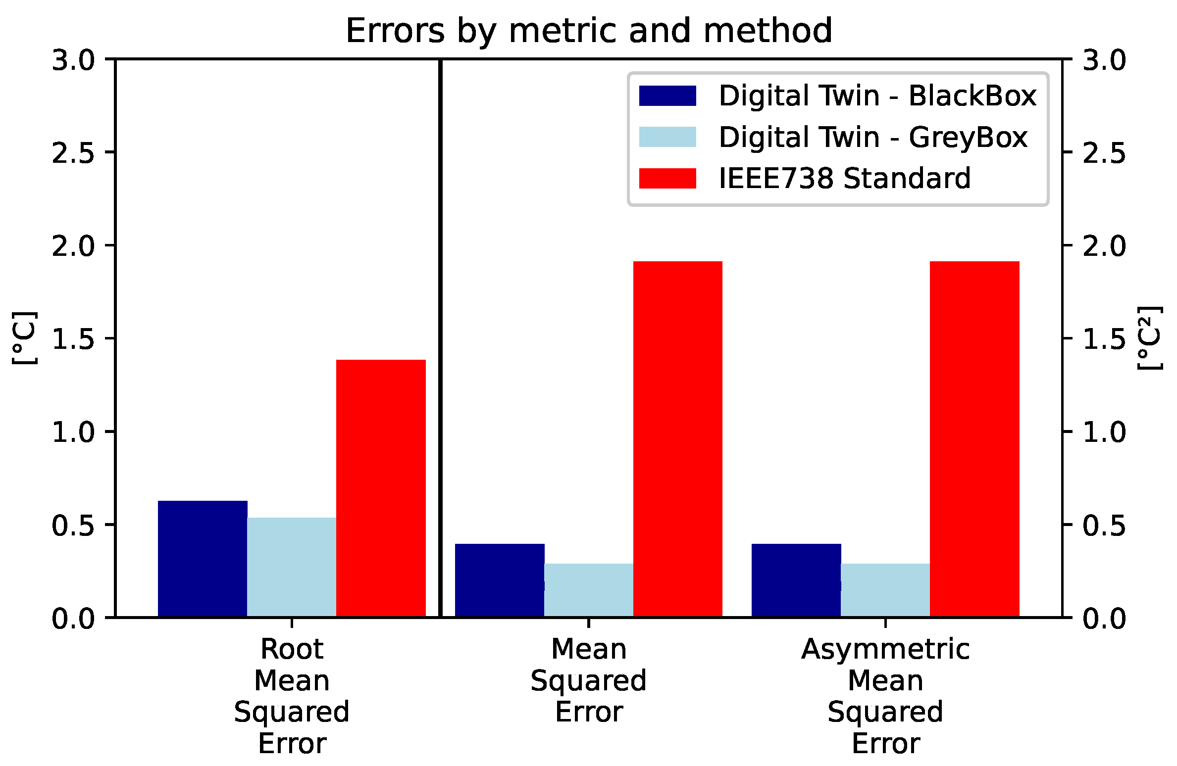
The first set of experiments, presented in
Section 4.1, encompasses the primary results of this work, comparing the Digital Twin approaches with the IEEE 738 standard. The main parameters of this experiment are the dimensionality of the problem
and the number of trees of a Random Forest
considered. The original number of features collected
S is 10, while the number of non-constant features
is 5, namely air temperature, sun irradiance, conductor current, wind speed, and wind direction.
, which is the default value of the model. For a proper validation of the performance metrics, 10-fold cross-validation is performed, i.e., the experiments are repeated 10 times by using a different training-set and testing-set. The size of the testing-set is 10% of the total data points: by adopting this technique, the performances over all the available data points can be measured.
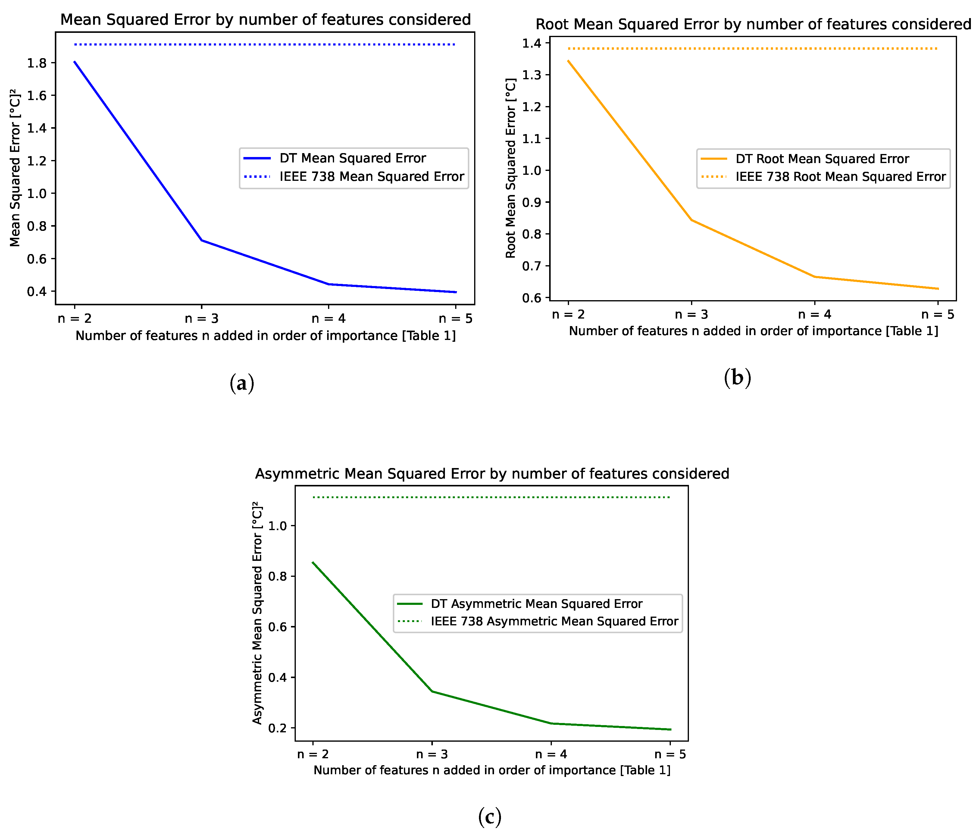
The second set of experiments explores possibilities provided by adopting a Digital Twin that goes beyond the forecasting of the conductor temperature. They show that it is possible to utilize a limited number of sensors without significant loss of prediction accuracy and heavily reduce the size of the training-set of the model. The first result is obtained employing Feature Selection, the process of selecting the most informative columns from a table of data. This can be achieved with many methods, one of them being the important features suggestions of a Random Forest Regressor. This particular value is computed by extracting the Gini impurity-based feature importances after fitting all the available data into the model, calculated explicitly as the normalized total reduction in the criterion brought by that feature. The higher, the more important the feature. The second result is obtained performing an iterative run of the black-box experiments by increasing the training-set size, starting with the 5% of the dataset (approximately four days), and increasing by 5% at each iteration.
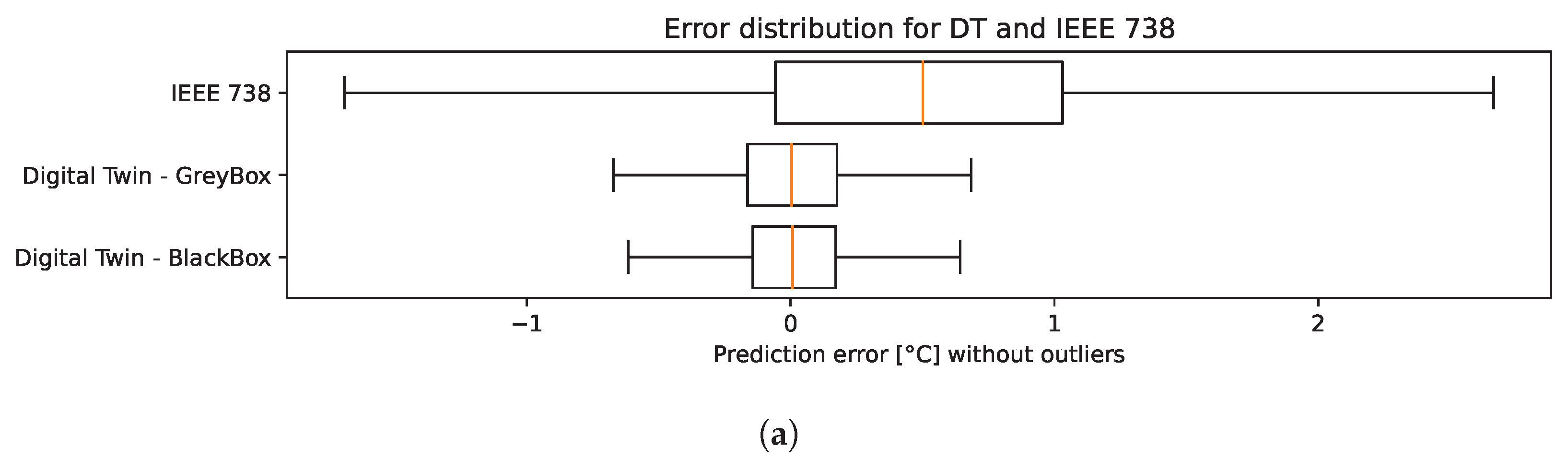
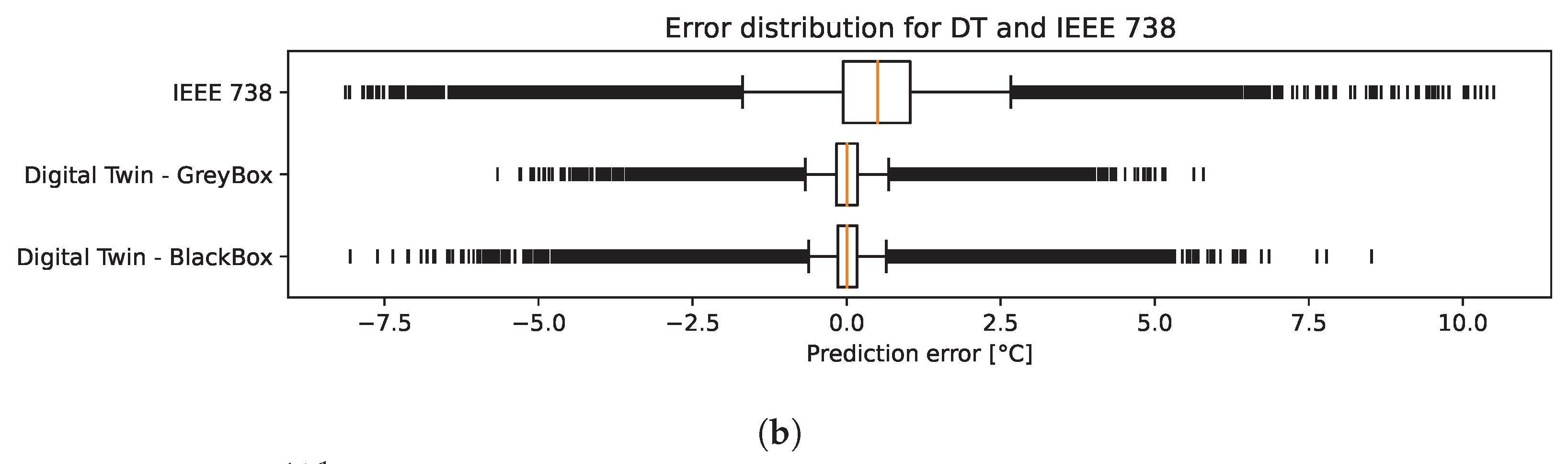
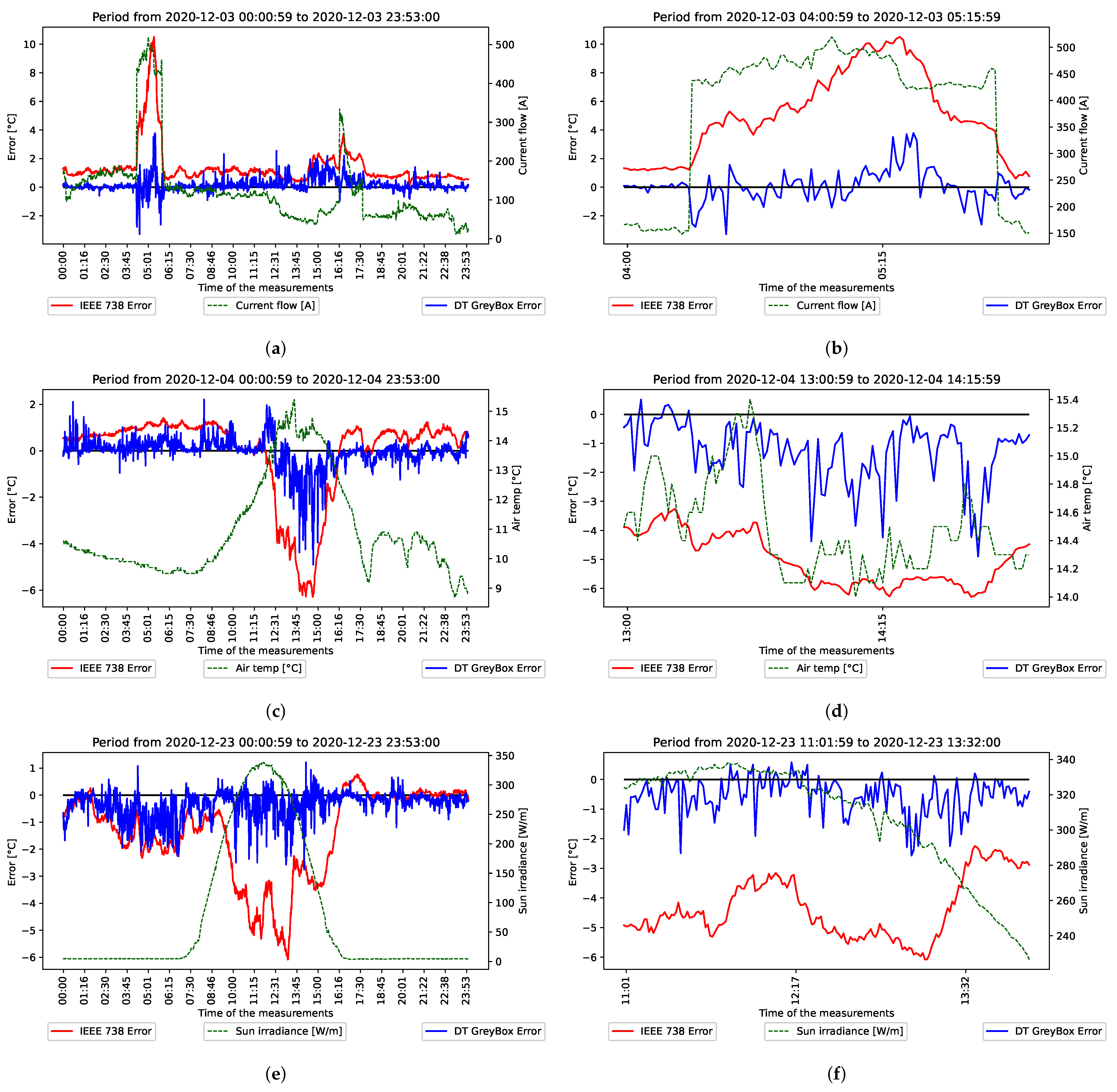
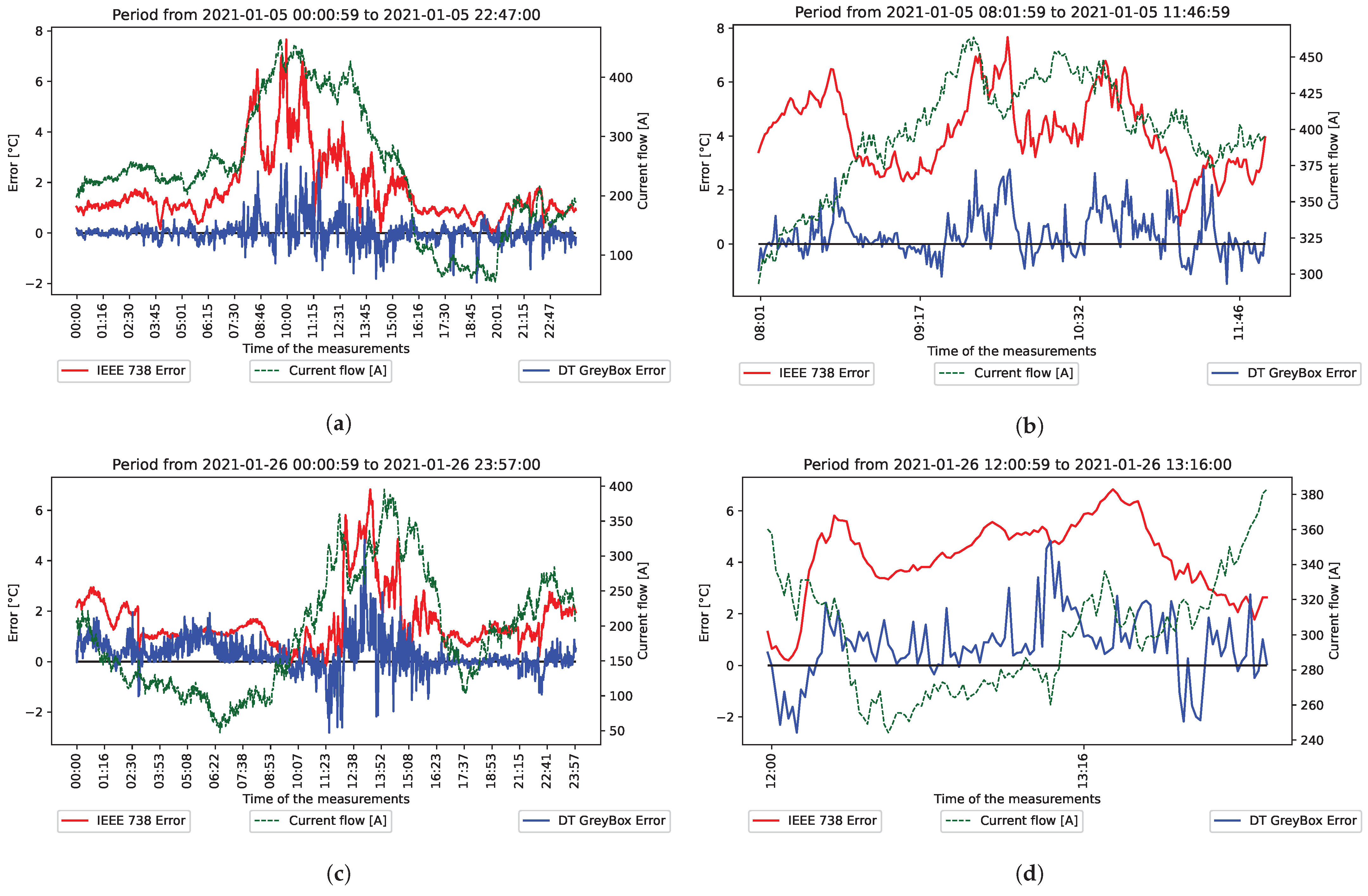
The last set of experiments aims at providing insights about physics-based model drawbacks. To achieve that, a correlational study was performed by filtering the days where an error greater than 5 °C in absolute value occurred for more than 40 measurements on the same day.
3.3. Metrics
Several metrics have been collected during these experiments. In the following, indicates the estimated value by any method, either , , or .
The prediction error at time
,
, is defined in Equation (
9). Traditional metrics, such as the mean squared error (MSE, (
10)) and the root mean squared error (RMSE, (
11)), do not consider the asymmetrical nature of the described problem. An underestimation of the conductor temperature can result in an excessive increase in the current flow yielding to safety risks: it must be penalized more than an overestimation. For this reason, an asymmetrical variation of the MSE, from [
35], is adopted and referred to as AMSE, defined in (
12), where
represents the desired degree of asymmetry, and
is a function whose value is 1 if the condition is true, 0 otherwise. For the reason mentioned above of penalizing underestimations,
is set to
, so that the corresponding MSE is multiplied by 0.75 for an underestimation and by 0.25 for an overestimation.
where
.
5. Conclusions
This work proposes a Digital Twin approach to support the Transmission Line Operators in dynamic thermal rating of overhead transmission lines. A maximal core temperature is established to ensure the safety of transmission lines. Several factors influence the internal conductor temperature, including the amount of current injected in the line, the air temperature, the solar irradiance, and the wind intensity. Because of the expensive nature of direct measurement sensors, it is crucial to accurately estimate the line temperature to adapt the current for optimal line usage.
Physics-based DTLR methods allow the estimation of a line core conductor temperature from weather and line sensors rather than using expensive direct measurements devices. Nevertheless, their adoption requires multiple sensors, and the needed computations are not adequate for real-time estimations. The proposed approach improves the quality of temperature estimation, diminishes the number of required sensors, and reduces general costs. It exploits temporary availability of direct temperature measurement for a training phase, and it is designed with two submodules: a black-box module and a grey-box module. The former tries to learn the mapping from the input sensors parameters to the actual conductor temperature, the latter from the input sensors parameters to the IEEE 738 error. Both modules significantly improve the estimation quality, with better results for the grey-box module. A comparison with the IEEE 738 standard shows a reduction of 60% of the Root Mean Squared Error and a decrease in the maximum estimation error from above 10 °C to below 7 °C with respect to the actual conductor temperature. Furthermore, by not relying on IEEE 738 measurements, the black-box module offers multiple advantages, including a significant dimensionality reduction with respect to the IEEE 738 standard. The experimental results, yet preliminary, suggest the adoption of data-driven approaches in conjunction with physics-based ones. Further studies will focus on the exploration of forecasting strategies by studying techniques to improve the estimation accuracy with a broader prediction horizon, as well as the simplification of the employed models for facilitating the adoption of a data-driven Digital Twin approach. Additionally, future research will focus on adopting transfer learning techniques for exploiting the existing models on new lines, reducing the need for data for modeling, with a further reduction in costs.


 ,
, 


