A New Self-Adaptive Teaching–Learning-Based Optimization with Different Distributions for Optimal Reactive Power Control in Power Networks


Department of Electrical Engineering, College of Engineering, Majmaah University, Al-Majmaah 11952, Saudi Arabia
Energies 2022, 15(8), 2759; https://0-doi-org.brum.beds.ac.uk/10.3390/en15082759
Submission received: 18 March 2022
/
Revised: 4 April 2022
/
Accepted: 7 April 2022
/
Published: 9 April 2022
(This article belongs to the Special Issue Electrical Power System Dynamics: Stability and Control)
Abstract
:Teaching–learning-based optimization has the disadvantages of weak population diversity and the tendency to fall into local optima, especially for multimodal and high-dimensional problems such as the optimal reactive power dispatch problem. To overcome these shortcomings, first, in this study, a new enhanced TLBO is proposed through novel and effective θ-self-adaptive teaching and learning to optimize voltage and active loss management in power networks, which is called the optimal reactive power control problem with continuous and discontinuous control variables. Voltage and active loss management in any energy network can be optimized by finding the optimal control parameters, including generator voltage, shunt power compensators, and the tap positions of tap changers, among others. As a result, an efficient and powerful optimization algorithm is required to handle this challenging situation. The proposed algorithms utilized in this research were improved by introducing new mutation operators for multi-objective optimal reactive power control in popular standard IEEE 30-bus and IEEE 57-bus networks. The numerical simulation data reveal potential high-quality solutions with better performance and accuracy using the proposed optimization algorithms in comparison with the basic teaching–learning-based optimization algorithm and previously reported results.
1. Introduction
An important part of efficient, affordable, and reliable power system operation, or in other words, optimal operation, is the optimal reactive power (Volt-VAR) control problem, which includes generator voltage, shunt compensator power, and the tap positions of tap changers [1]. In a competitive and deregulated environment, the optimal Volt-VAR control issue is an important and efficient tool in electrical energy transmission networks. The main objective of solving the Volt-VAR control issue is to reduce network losses and, as a result, reduce the final cost of energy transmission in energy systems while satisfying a set of operational and physical constraints imposed by network and equipment limitations. The basic goal is to minimize essential key functions, such as the summation of bus voltage deviations and active power losses while also addressing several practical limitations [2]. Because generator voltage is intrinsically continuous but shunt reactive power compensators and tap changer ratios are discrete variables, the optimal VAR control problem is viewed as a complex multimodal nonlinear optimization issue including discrete variables. This problem is also a multimodal, high-dimensional, and complex sophisticated problem with some nonlinear objective functions with multiple local minima and several nonlinear and discontinuous constraints [1,2,3,4].
Numerous methods, ranging from standard mathematical techniques to those related to artificial intelligence, have been proposed over the past years for the application of optimal VAR control problems. The introduction of the harmony search algorithm (HSA) is an example of development in this area [5]. Additionally, Roy demonstrated the increased capability of the biogeography-based optimization (BBO) method for solving multi-constrained problems [6]. In addition, differential evolution (DE) with dynamic multi-group self-adaptive operators (DMSDE) [7], particle swarm optimization (PSO) based on multi-agent systems (MAPSO) [8], fuzzy adaptive PSO (FAPSO) [9], DE [10], and comprehensive learning PSO (CLPSO) [11] are other works in this area. Other approaches such as the seeker optimization algorithm (SOA) and a distributed Q-learning method were also discussed in [12,13], while in [14] a stochastic problem was solved using quasi-oppositional teaching–learning-based optimization (TLBO) [15], named QOTLBO.
To solve diversified integer nonlinear issues such as minimizing the L index and power losses at the same time, chaotic enhanced PSO-based techniques such as MOCIPSO and MOIPSO were presented in [16]. In Reference [17], different ways of tackling the reactive power planning (RPP) problem were thoroughly explored. Ref. [18] examined various significant practical limitations of the optimal power flow (OPF) issue, highlighting three in particular: the valve-point effect, the multi-fuel option, and, most critically, the forbidden operating zone. A soft computing technique based on differential evolution application of a new voltage stability index (NVSI) was developed in [19] to detect weak buses in the RPP problem. To increase voltage stability, improve the voltage profile, and reduce network losses, Reference [20] used chemical reaction optimization (CRO) to allocate a static synchronous compensator (STATCOM). The Gaussian bare-bones TLBO (GBTLBO) algorithm was presented in [21] to address ORPD. Using a nature-inspired design termed the water cycle algorithm (WCA), the ORPD problem was resolved in [22]. In [23], to optimize the solution to the ORPD problem, moth-flame optimization (MFO) was successfully applied; this optimizer was inspired by moths’ night-time navigation method, in which they employ visible light sources for guidance. In [24], to accomplish various goals of ORPD, an improved social spider optimization (ISSO) algorithm was recommended. Semidefinite programming (SDP) has recently received a lot of attention in the power system research community. Under certain technical constraints, a new SDP design was exploited in [25] to propose a unique equivalent convex optimization formulation for the ORPD problem. Moreover, in [26], the application of a well-known technique, i.e., grey wolf optimizer (GWO), was deployed to address the ORPD issue.
In addition to the approaches listed above, many other optimizers have been utilized to tackle optimal Volt-VAR control via various systems with single and multiple objectives. These methods include tight conic relaxation [27], pseudo-gradient search based on PSO (PSO-IPG) [28], hybrid DE and PSO [29], a hybrid imperialist competitive algorithm (ICA) and PSO (HPSO-ICA) [30], artificial bee colony (ABC) with chaotic (CABC) and DE (CABC-DE) [31], a developed gravitational search algorithm (GSA) with conditional selection strategies (CSS) (IGSA-CSS) [32], ant colony optimization (ACO) [33], a modified stochastic fractal search (MSFS) [34], improved ant lion optimization (IALO) [35], the whale optimization algorithm (WOA) [36], adaptive chaotic symbiotic organisms search (A-CSOS) [37], a hybrid GSA and PSO (HPSO-GSA) [38], the Gaussian bare-bones water cycle algorithm (NGBWCA) [39], fractional-order Darwinian PSO (FO-DPSO) [40], the exchange market algorithm (EMA) [41], the differential search algorithm (DSA) [42], ant lion optimization (ALO) [43] and, new colliding bodies optimization (ICBO) [44], JA (JAYA algorithm) [45], the two-archive multi-objective GWO (MOGWA) [46], ABC with firefly (ABC-FF) [47], the crow search algorithm (CSA) [48], a new version of PSO [49], SARGA [50], and a new version of DE [51].
Rao, Savsani, and Vakharia introduced the TLBO algorithm in 2011 [15], which is based on teaching and learning operations. The optimal VAR control issue, on the other hand, includes the aforementioned features. As a result, there is a critical need for a sustainable global approach to power system optimization. The simulation results demonstrate that these improved θ-self-adaptive teaching and learning (θ-SATLBO) algorithms employing alternative distributions converge to more optimal solutions than previously published techniques.
In general, the author attempted to create better optimization algorithms for discovering better optimal solutions than earlier published methods. Almost all demonstrations are based on the quality of the effective solutions and the converging characteristics of the best run out of many runs. In the second section of this article, the standard formulation of the optimal VAR control issue is discussed, whereas in the third section, the arrangement of θ-SATLBO is explained. The next section summarizes the simulation results and compares and analyzes the methodologies utilized to address use cases of optimal VAR control problems. Finally, the concluding paragraph of this paper summarizes the implementation of the recommended algorithms.
The rest of this paper is organized as follows. Section 2 presents the Volt-VAR control formulation for optimization. Section 3 presents the new proposed algorithms for the optimal VAR control problem. Section 4 shows the obtained optimal numerical results of the optimal VAR control problem. Finally, Section 5 presents the conclusions.
2. Volt-VAR Control Formulation
For the most part, a solution to the optimal VAR control (Volt-VAR control) problem aims at minimizing the sum of bus voltage deviation (SVD) while optimizing active losses (Ploss) in the power grid, though some important criteria must also be fulfilled [1,2,3,4].
The following are the mathematical equations for formulating the optimal VAR control issue [21]:
Subject to:
The objective function, which should be minimized, is , and represents the dependent variables, including:
- Load voltage VL;
- Unit reactive power QG;
- Network line loading limit Sl.
As a result, the vector can be defined as follows:
NG signifies the number of units, and is the vector of independent continuous and discontinuous decision parameters, including [21]:
- Unit voltages VG;
- Transformer taps T;
- Shunt reactive sources QC.
As a result, it is represented as:
2.1. Optimal VAR Control Functions
2.1.1. Network Active Loss Reduction
The objective of the optimal VAR control problem is to minimize the real power transmission losses ) in the transmission network. Total network active losses in system power are significant because the magnitude of current flowing through conductors is high, and the length of transmission lines can be up to hundreds of kilometers. In order to reduce network active losses, the optimization of network active losses is an important solution. The network active loss reduction function is described as follows:
All of the parameters in the above equation, including NPQ, PQ, δij, NTL, and gk, are defined in [21].
2.1.2. Minimization of SVD
Bus voltage is regarded as a critical security and service indicator. In this situation, the goal function for the optimal VAR control issue is the minimization of SVD. The objective function is as follows:
2.1.3. Minimization of Both Objective Functions (Optimal VAR Control Problem)
In an optimal VAR control problem, using only a true power loss objective will result in workable control parameters with an unsatisfactory voltage profile. The optimal VAR control function is as follows:
Here, λ is the penalty factor, which is designated as 0.7 and 0.8 for the two standard IEEE test systems, respectively.
2.2. Constraints
2.2.1. Equality Constraints
The following are some illustrations of typical load flow equations with as the equality constraint [21]:
All of the parameters in the above equation, including PGi, NB, QGi, QDi, PDi, Bij, and Gij, are defined in [21].
2.2.2. Inequality Constraints
The inequality constraints of the problem, , are as follows:
- Generation units’ constraints: The base unit power at the base bus ( and ), the voltages of the generation units’ bus ( and ), and the generation units’ reactive power ( and ) are all constrained by the following limitations (for ):
- Tap-changer trans limitations: The settings for tap-changer trans taps (T) are constrained by their minimum and maximum limits, respectively:where and define higher and lower tap limits of the ith tap changer.
- Network parallel compensator’s reactive constraints: Compensations for parallel VARs are constrained by the following limits:
- Constraints on security: These include voltage restrictions on transmission line loading () and load buses:
The objective function (Cost) imposes penalty terms on dependent variables. Thus, (1) is modified as follows [5]:
where and are penalty terms, and the number of load buses and generator buses in which voltage and injected reactive power are outside the limits ( and ) and are clearly characterized as:
3. Improved Optimization Algorithms
3.1. TLBO
The TLBO optimizer, which was introduced in [15], is a well-known optimizer. Because of the TLBO algorithm’s foundation in simulating an old-school learning process, it is easy to understand how it works. There are two stages of learning in this process: learning from a teacher and learning by engaging with other students or learners (known as the learner phase). There are varieties of decision variables that are used as knowledge topics for a group of learners in this optimization technique. The “fitness” value is equal to the result of a learner. The teacher is often regarded as the best option for the needs of the entire community. Since the problem parameters are essential variables in the optimization problem’s objective function, a good solution is one that maximizes this objective function to its optimal value. Both portions of the TLBO algorithm are executed sequentially. The “teacher phase” of the algorithm comes first, followed by the “learner phase”.
3.1.1. Teacher Phase
During this phase, the best particle (or teacher) strives to improve the class’s average outcome in the subject that he or she teaches, within the limits of his or her competence. Obviously, at this phase, the teaching position is allocated to the most qualified member (teacher). Thus, enhancing the mean outcome of the class in the TLBO method is analogous to improving other individuals () by repositioning them closer to the teacher’s position while taking the existing mean value of the people into account (). Each parameter in the problem dimension is given an average value, and this technique perfectly reflects the quality of all present learners in the population. Equation (19) demonstrates how the gap between the teacher’s understanding and the quality of the learners or other populations might affect the students’ quality improvement.
TF denotes a teaching factor in the introduced equation determining the value of the average to be adjusted, and r is a random value in the range [0, 1].
The value of TF should be either 1 or 2, which is selected heuristically and randomly with equal probability using: .
3.1.2. Learner Phase
Learners should promote their understanding in two different ways: by receiving input from the teachers or through interactions among themselves, which is termed the learner phase. During this process, attempts to progress his/her understanding via peer learning from a random learner , where is not equal to . Two possibilities can occur subject to the values of and : if has more understanding than , then is moved towards (Equation (20)). Then, it is moved away from (Equation (21)). If has better functionality according to Equation (20) or (21), it will be allowed into the community. The TLBO optimizer will continue producing generations until it reaches the final iteration.
Students or learners can enhance their knowledge in two ways: through teacher input or through peer engagement, referred to as the learner phase. During this step, student i () tries to increase its understanding via peer learning from unrelated people (), where i is not equal to ii. Two possibilities exist subject to the values of and : if is greater than , is shifted toward (Equation (20)). If not, it is shifted away from (Equation (21). If the performance of a new learner () is superior to that predicted by Equation (20) or (21), it will be allowed into the community.
Additionally, it is vital to successfully deal with implausible learners to evaluate whether one learner is superior to any other learner when run on engineering optimization functions.
3.2. Mutation Operators for Improved Algorithms
When using the TLBO method, one should be aware of potential problems such as slow convergence, early convergence, poor accuracy, and a lack of diversity. The TLBO algorithm’s effect is improved by using three well-known mutation techniques as upgraded phases. Mutation operators bring in new students by changing the behavior of an existing one, hence increasing diversity in the classroom and decreasing the likelihood of the search becoming trapped in local optima. Random distribution sequences can have Gaussian, Lévy, Cauchy, or Beta distributions, as well as chaotic distributions based on logistic maps or mixed types such as a cloud distribution. Personal and globally optimal position vectors, as well as randomly picked current positions and speeds, can be altered. In this section, we describe three different types of mutations that we use throughout the paper.
3.2.1. Cauchy Mutation Using Cauchy Distribution
There is also the Cauchy distribution [52], which has the probability density function as a distribution:
where t > 0 is a scale variable and x ∈ R. To show that Y (a real-valued random parameter) is Cauchy-distributed with t > 0, the parameter Y for this distribution is as follows:
The Cauchy mutation using the Cauchy distribution for t = 1 is as follows:
where Learneri(d) is the dth control parameter of the ith learner, and δd(1) shows that the random value is newly created for any position of d.
3.2.2. Gaussian Mutation Using Gaussian Distribution
One of the most widely used distributions is the Gaussian distribution [52]. It is a simple distribution and is described by its mean μ and variance σ2. The formula for this probability density function is as follows:
A parameter Y is shown to be normally distributed as follows:
Then, the Gaussian mutation using the Gaussian distribution for σ = 1 and μ = 0 is created as follows:
where Nd(0, 1) specifies that every time a value is entered, a new random number is created.
3.2.3. Lévy Mutation Using Lévy Distribution
A probability density function can be expressed analytically for the Lévy distribution [53]. To express the Lévy distribution, the formulas below are used:
The Lévy mutation [54] using Lévy distribution with γ = 1 and = 1 is created as follows:
where indicates that the random number is newly generated for each value of d.
3.3. Improved TLBO Algorithms with Mutation Strategy
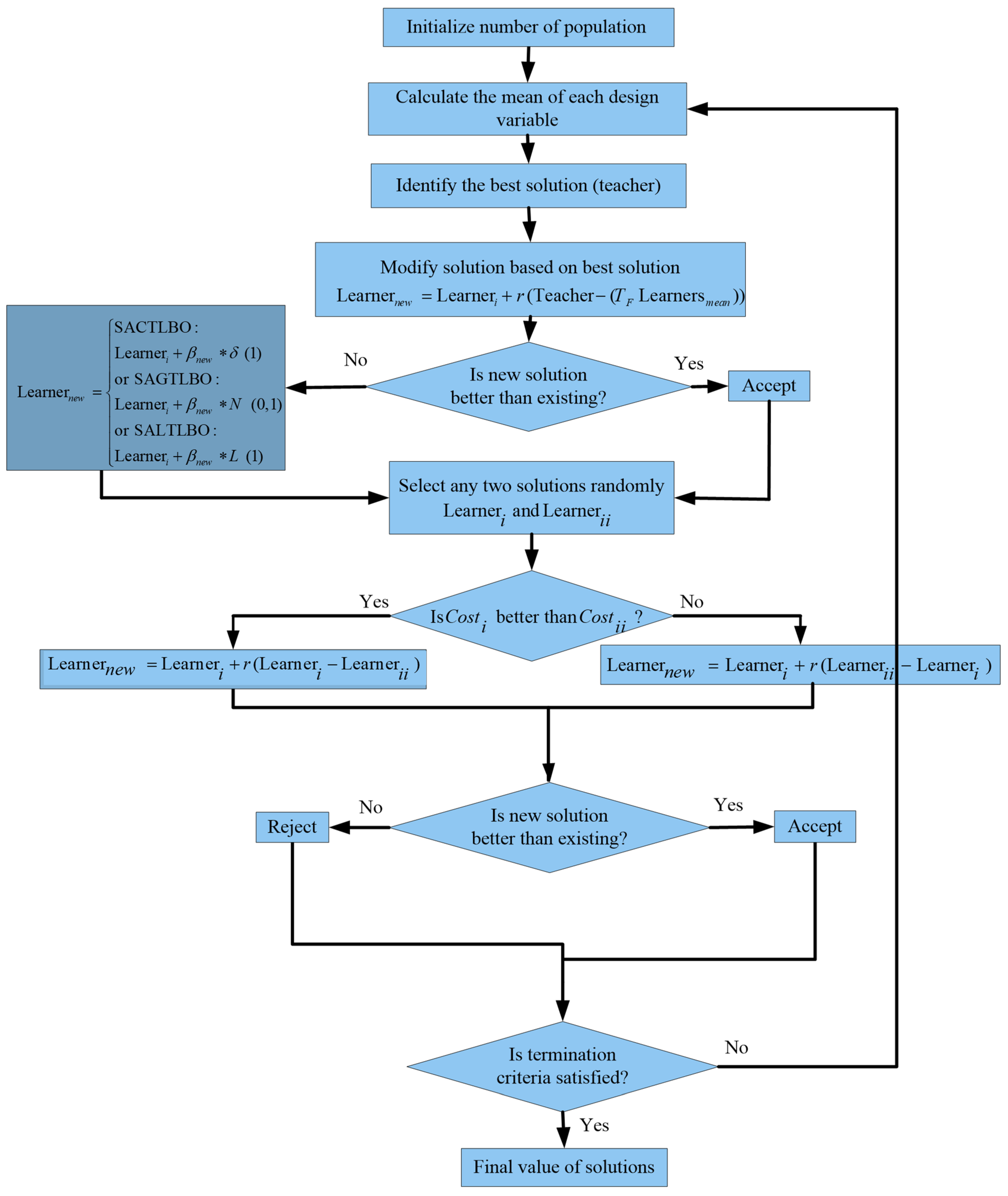
The updated and improved algorithm produces a better-simulated response and performs better in global and local search factors. Figure 1 illustrates how effective the hybrid method is. It is possible that students will be subjected to self-adaptive mutations in the hybrid phase of the new algorithm if they do not perform well in teacher phase tests.
3.4. Self-Adaptive Strategy in TLBO
In enhanced algorithms, students seek difficulties in their space using learning and education activities and shifting a random percentage of their distance from the teacher and other students in each repetition. By selecting excellent initial values for auxiliary mutation parameters, students can proceed more quickly toward global optima and cross local optimum points. However, when students approach global optima, the algorithm is unable to perform an effective local search since the parameters are greater than the search space.
When initial values for auxiliary mutation parameters are kept minimal, the algorithm can perform a local search with a high degree of stability and strength. However, in this instance, students progress slowly toward the goal, and their ability to cross over local optimal spots diminishes. As a result, we must exert control over auxiliary mutation parameters to boost the functionality of improved methods in global and local searches while simultaneously decreasing the value of auxiliary mutation parameters via increased repetition time. To increase the performance of mutations, we employ a comprehensive technique based on sigma adaptation to several parameters.
The self-adaptive variance approach is used by selecting a β parameter vector with the length of the problem dimensions. Here, the β parameter mutates first, and then other members mutate using this new parameter. The essential relationship is defined as follows:
In the above relationship, τ′ is defined as the “global learning rate” and is obtained by , and τ is defined as the “learning rate of different characteristics of vector” and is determined by the relationship , where indicates the maximum number of authorized algorithm execution or generation production periods. The remaining requirements are identical to those in the previous method. As a result, Equations (19)–(21), (24), (27), and (29) self-adapt and are used:
Combining SATLBO with mutation operators leads to the following new advanced and powerful optimizers:
- SACTLBO: The SATLBO algorithm was improved through the application of Cauchy mutation.
- SAGTLBO: A Gaussian mutation-based improvement was applied to the SATLBO algorithm.
- SALTLBO: The SATLBO algorithm was improved by the application of Lévy mutation.
3.5. θ-SATLBO Optimizers
Rather than optimizing the real space of control variables, phase-angle optimization is at the heart of our approach. Ultimately, the approach generates an answer similar to a phase angle, from which the last values of the decision parameters are deduced. As a result, formulations 31 and 36 are altered as follows:
Decision parameters are constrained to (−π/2, π/2) values in this approach. Angle phases are included in the problem-solving process implemented by the hybrid θ-SATLBO algorithm. Phase angles are changed for each repetition through formulations (37) to (42), and at the end, control variables are determined by the mapping below:
This is a one-to-one mapping extender. The intended mapping can be used to map real limits of the optimization function to a θ space, and inverse per-unit systems simplify the calculation and understanding of the problem because of this mapping. Due to the compressed θ space versus the actual problem space, the θ values are negligible, and the effectiveness of the resolution rises significantly. As a result, in a compact space such as θ space, the algorithm’s local optima may be extremely close to the global optima.
4. Numerical Results of Optimal VAR Control Problem
The suggested procedures based on the optimal VAR control issue were evaluated on two standard power networks to verify their efficiency. TLBO optimizers were built in MATLAB 7.6 on a Pentium IV E5200 PC with 2 GB of RAM, and the simulation was performed. The chosen values of the final iterations () for two power systems, 30- and 57-buses of standard IEEE networks, were 100 and 150 with population sizes of 45 and 60, respectively.
There are discontinuous parameters with a step value of 0.01 p.u. for shunt compensators and transformer taps’ reactive powers, and penalty values in (16) are fixed at 500 [12]. The following algorithm results represent the best possible solutions over 50 independent trails.
4.1. The First Test Network: IEEE 30-Bus Power Network (System 1)
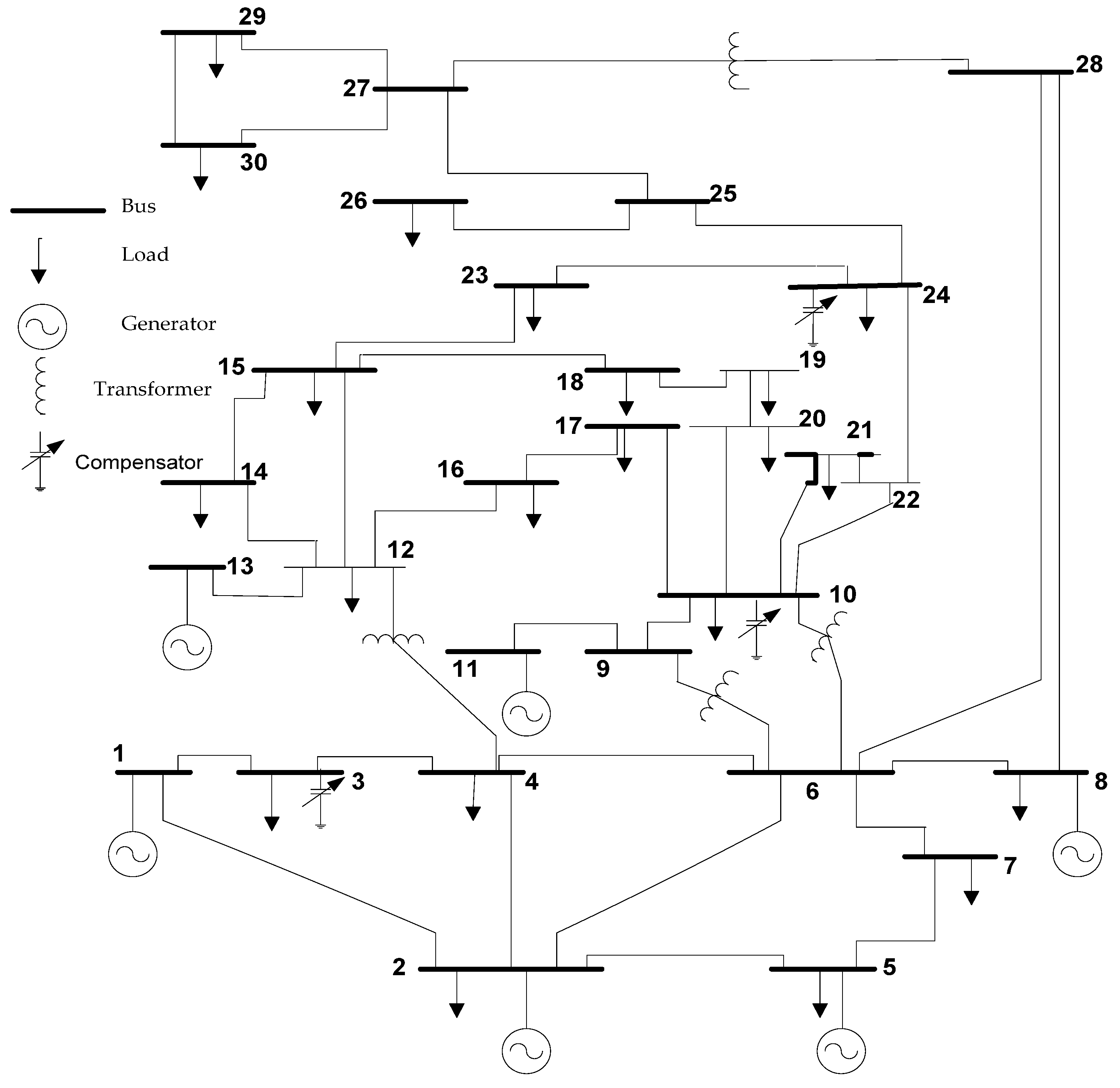
In this part, simulation outcomes derived from the solution of the optimal VAR control issue using the provided techniques are discussed. The proposed new TLBO optimizers’ performance was evaluated using the IEEE 30-bus standard depicted in Figure 2. Reference [7] described the IEEE 30-bus network and its primary working limits and situations. Table 1 shows the allowed ranges of decision variables. Six generators were situated on buses 1, 2, 5, 8, 11, and 13 in the IEEE 30-bus test system. Additionally, buses 3, 10, and 24 were designated as active compensatory shunt buses [8].
The network loads were specified as:
Qload = 1.262 p.u., Pload = 2.834 p.u.
The entire primary units and network losses were defined as:
∑QG = 0.980199 p.u., ∑PG = 2.893857 p.u., Qlosss = −0.064327 p.u., Ploss =0.059879 p.u.
The proposed algorithms’ viability was evaluated using various goal functions on this test network, as explained below.
4.1.1. Minimization of Network Active Losses
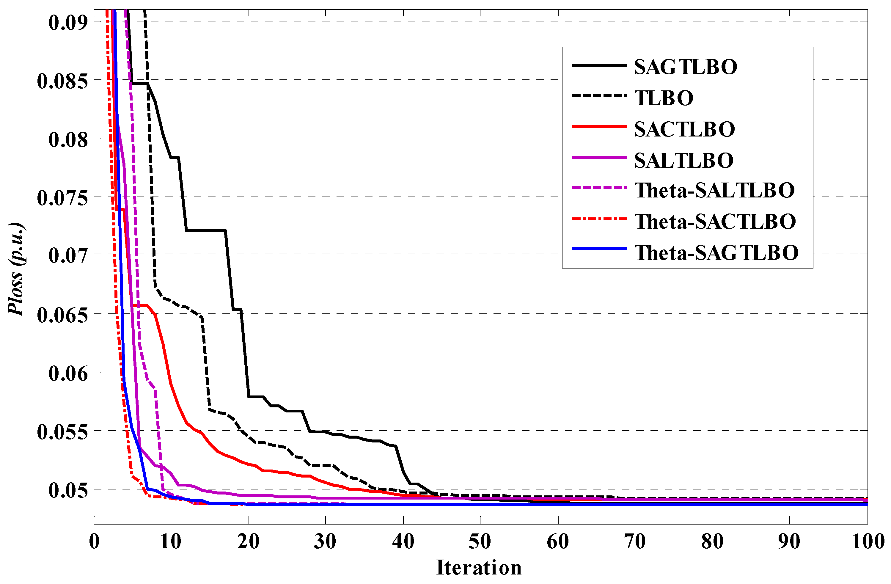
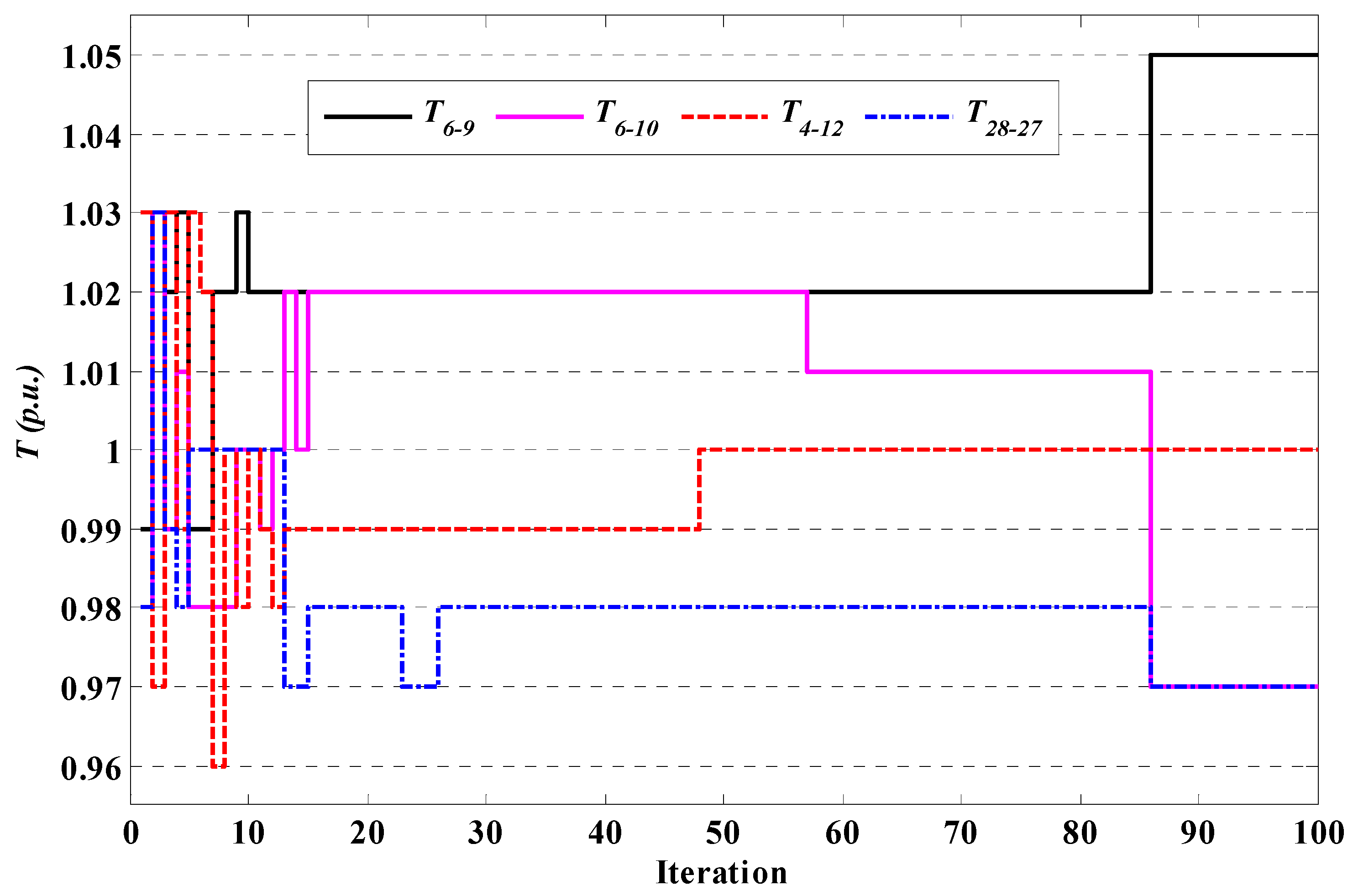
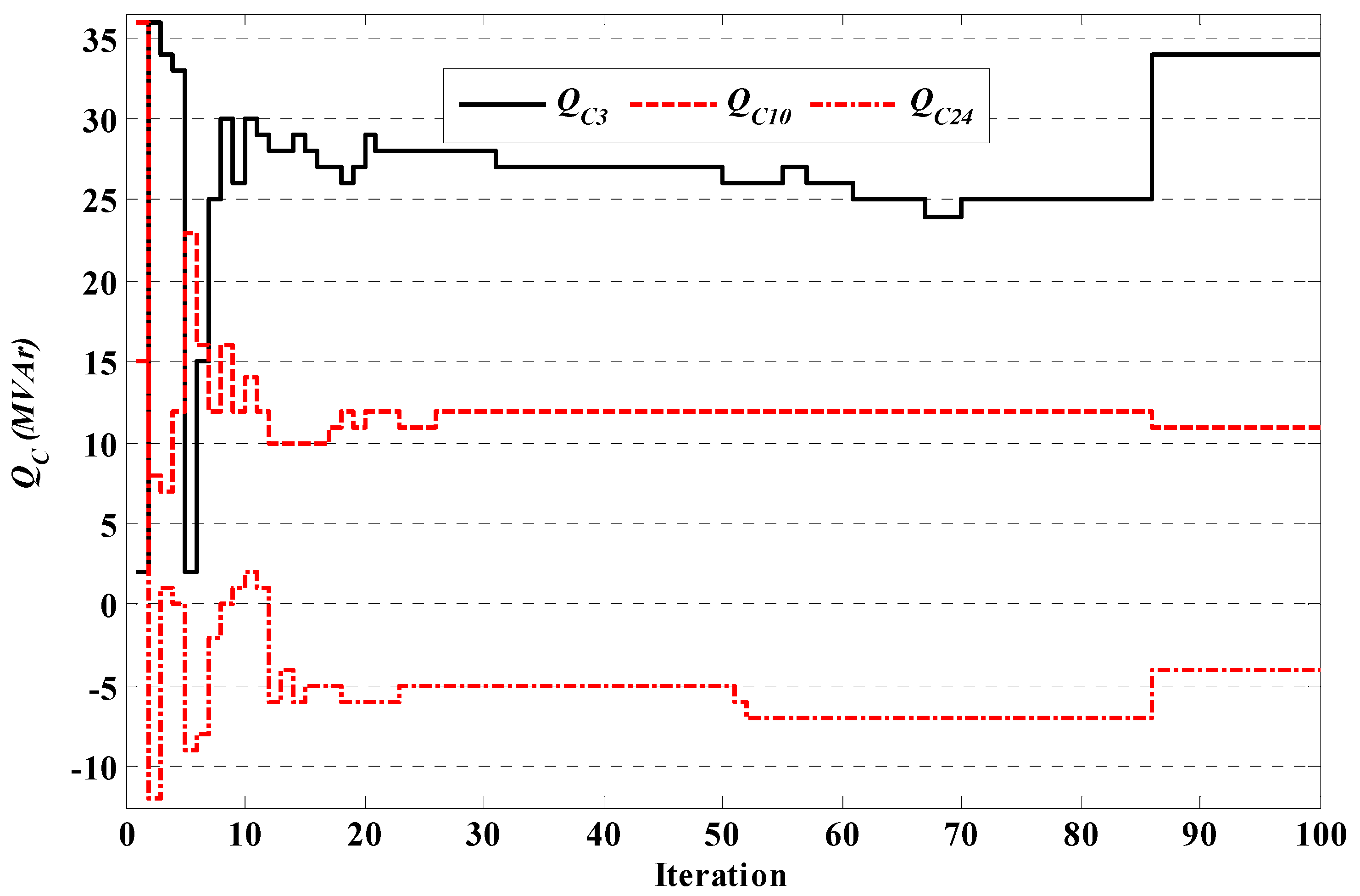
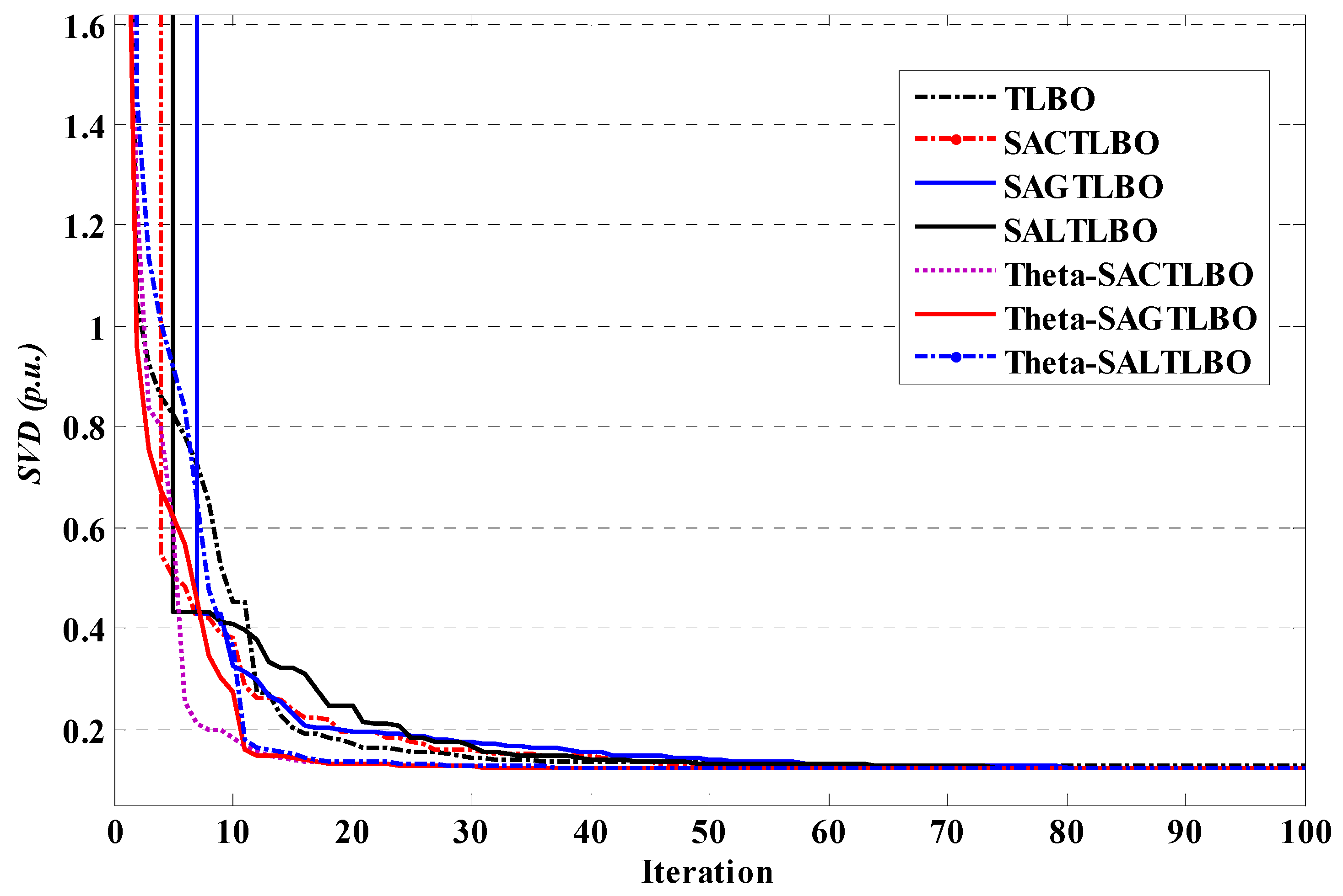
The goal is to reduce total transmission losses to a minimum. Table 2 summarizes 50 trials’ best optimal VAR control problem solutions for minimizing actual total transmission power losses using θ-SAGTLBO. The results indicate that using θ-SAGTLBO leads to active power losses of 0.0486217 p.u., which is smaller than the amount achieved using other methods. When evaluating convergence characteristics, Figure 3 demonstrates that θ-SATLBO optimizers achieve a better set of control parameters more quickly than other TLBO optimizers.
Table 3 compares the specifications of the ideal situations acquired by the suggested algorithm techniques after 50 runs to those obtained by the references. A summary of operation symbols, including the mean execution times, the best (Best) and poorest (Worst) real losses, the standard deviation (Std.), the average real losses (Mean), and loss saving percentage (Psave) over 50 independent runs, are shown in the following table. Table 3 shows that the θ-SAGTLBO strategy reduces active power loss by 18.81%, the largest reduction in losses compared with other alternatives. According to the outcomes, the θ-SAGTLBO algorithms outperform other algorithms in terms of resilience.
4.1.2. Improvement of the Voltage Profile
In this function, the goal function for the optimal VAR control issue is the minimization of voltage deviation (SVD). The optimal control variable settings found using the various methods for case 2 are summarized in Table 4. Each algorithm’s final solution and CPU time were monitored, and substantial statistical data are provided in Table 5. As shown in Table 4, the suggested θ-SACTLBO and θ-SAGTLBO algorithms produce an SVD of 0.1233 p.u. In terms of the features of the solutions, the results clearly show that the presented SAGTLBO algorithms trump the other state-of-the-art methods. The convergence features of the voltage deviation minimization method using the TLBO algorithms are plotted in Figure 7.
4.1.3. Improvement of the Network Voltage Profile with the Minimization of Active Losses
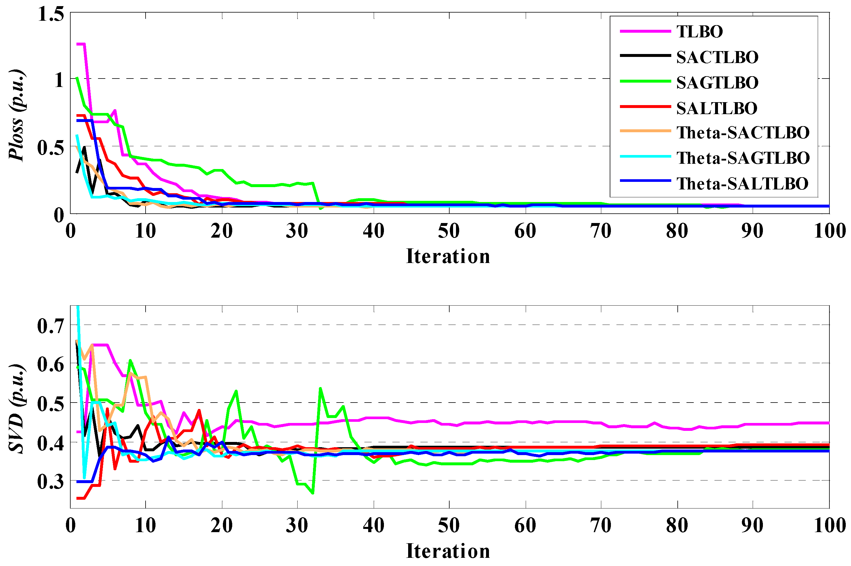
Instead of optimizing the SVD and losses separately, the algorithms optimize both together. Table 6 summarizes the optimal control variables, SVD, and power losses associated with the methods. As can be seen from the data, the updated algorithms discovered the optimal tradeoff between active power losses and SVD. The convergence rate of SVD and loss minimization is presented in Figure 8 for all TLBO optimizers. The active power losses in this scenario are greater than those in case 1 and less than those in case 2, although SVD is superior to case 1 and inferior to case 2.
4.2. The Second Test Network: IEEE 57-Bus Power Network (System 2)
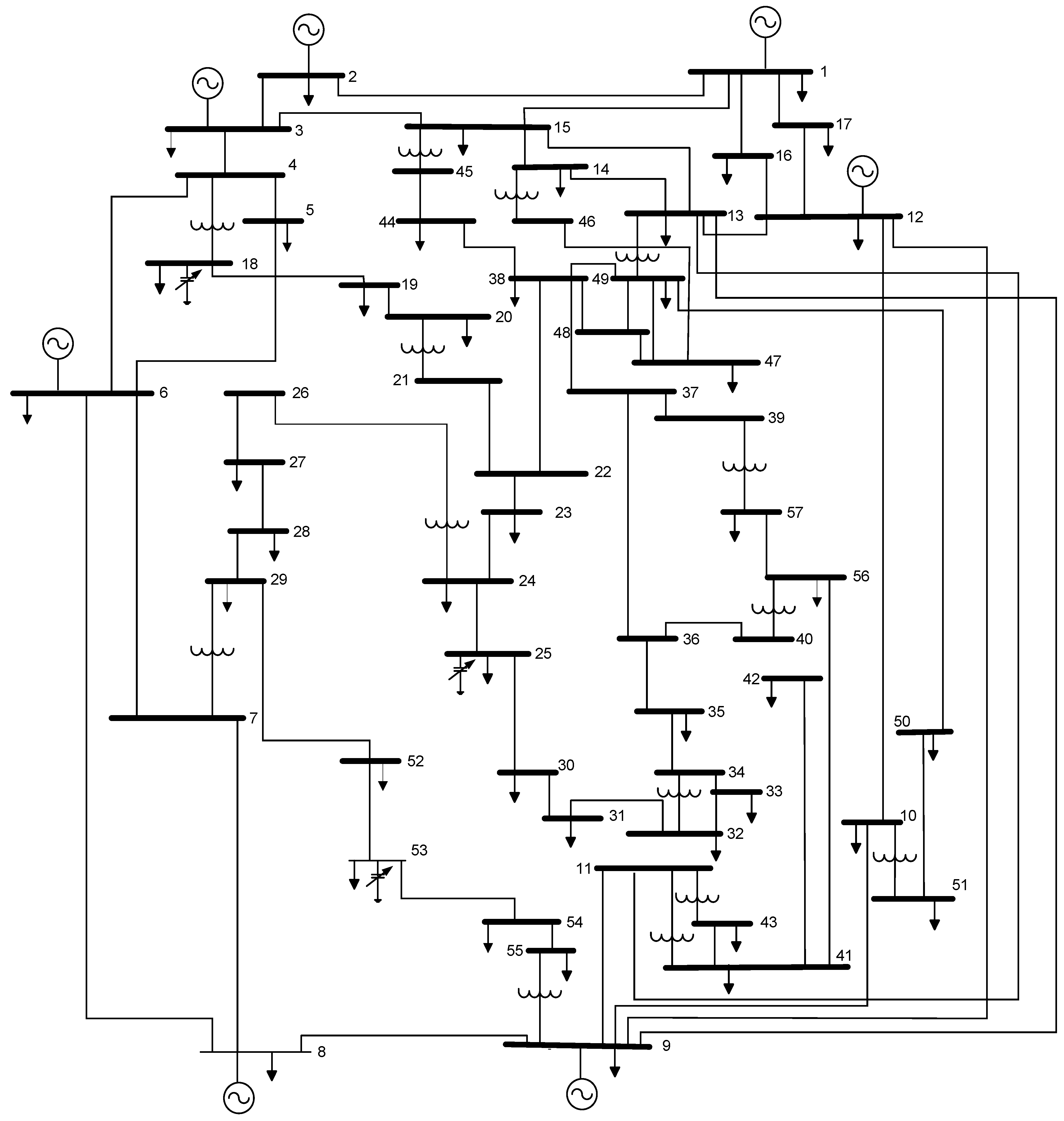
This system, as shown in Figure 9, is presented as a large-scale network for the second step of the optimal VAR control issue to show the usefulness of the proposed algorithms in larger-scale systems. Eighty transmission lines with buses 18, 25, and 53, parallel reactive power generators, and seven generators on buses 1, 2, 3, 6, 8, 9, and 12, as well as fifteen load tap setting transformer branches, make up the test system being investigated. The bus statistics, the line data, and the allowed range of real power generation were obtained from Reference [12], and the parameter limitations are shown in Table 7.
The network loads are [58]:
Qload = 3.364 p.u., Pload = 12.508 p.u.
The entire primary units and network losses obtained are [58]:
∑QG = 3.4545 p.u., ∑PG = 12.7926 p.u., Qlosss = −1.2427 p.u., Ploss =0.28462 p.u.
4.2.1. Minimization of Network Active Losses
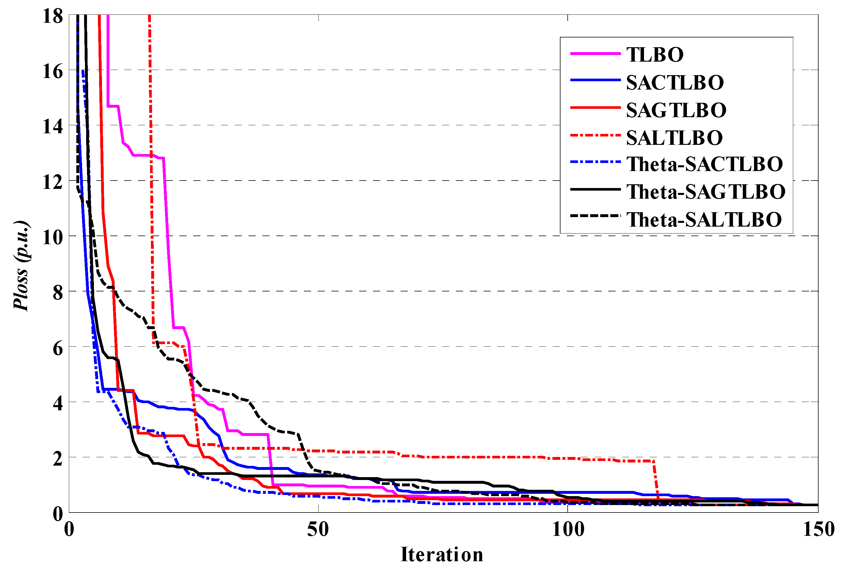
Table 8 presents the statistical information and CPU time of the ideal settings found using various methods. The θ-SAGTLBO algorithm determined the optimum solution after 50 trial runs. The active power losses produced by the θ-SAGTLBO algorithm are shown to be 0.2372619 p.u. In this table, we can see that the θ-SAGTLBO method achieves a 16.64 percent reduction in power loss, which is greater than the other alternatives. The assessment of the resilience of the suggested simulation methodology is based on data from 50 separate runs with diverse initial populations. Obviously, θ-SAGTLBO shows a more robust and effective performance than other methods. To ensure a close-optimal response in any randomized attempt, the Std. index across several trials must also be extremely low. Figure 10 depicts the convergence rates for network losses as a function of iteration number.
4.2.2. Improvement of the Voltage Profile
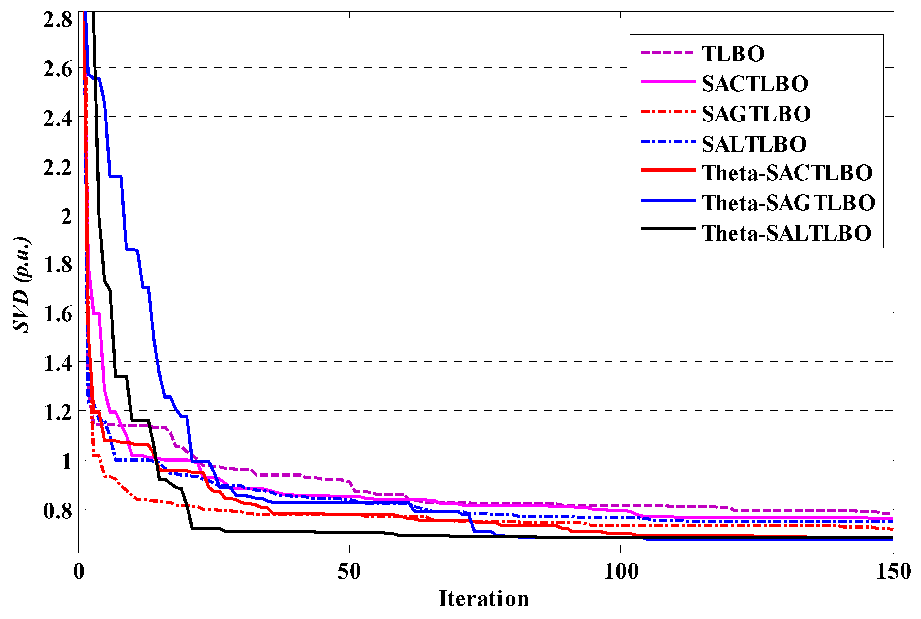
This experiment assessed the objective function of SVD reduction for this network. Table 9 illustrates the statistical information and CPU time for the various algorithms. The SVD obtained by the θ-SAGTLBO method is the best result for this case, as depicted in Table 9. The algorithm convergence rate of voltage deviation minimization is illustrated in Figure 11.
4.2.3. Improvement of the Network Voltage Profile with the Minimization of Active Losses
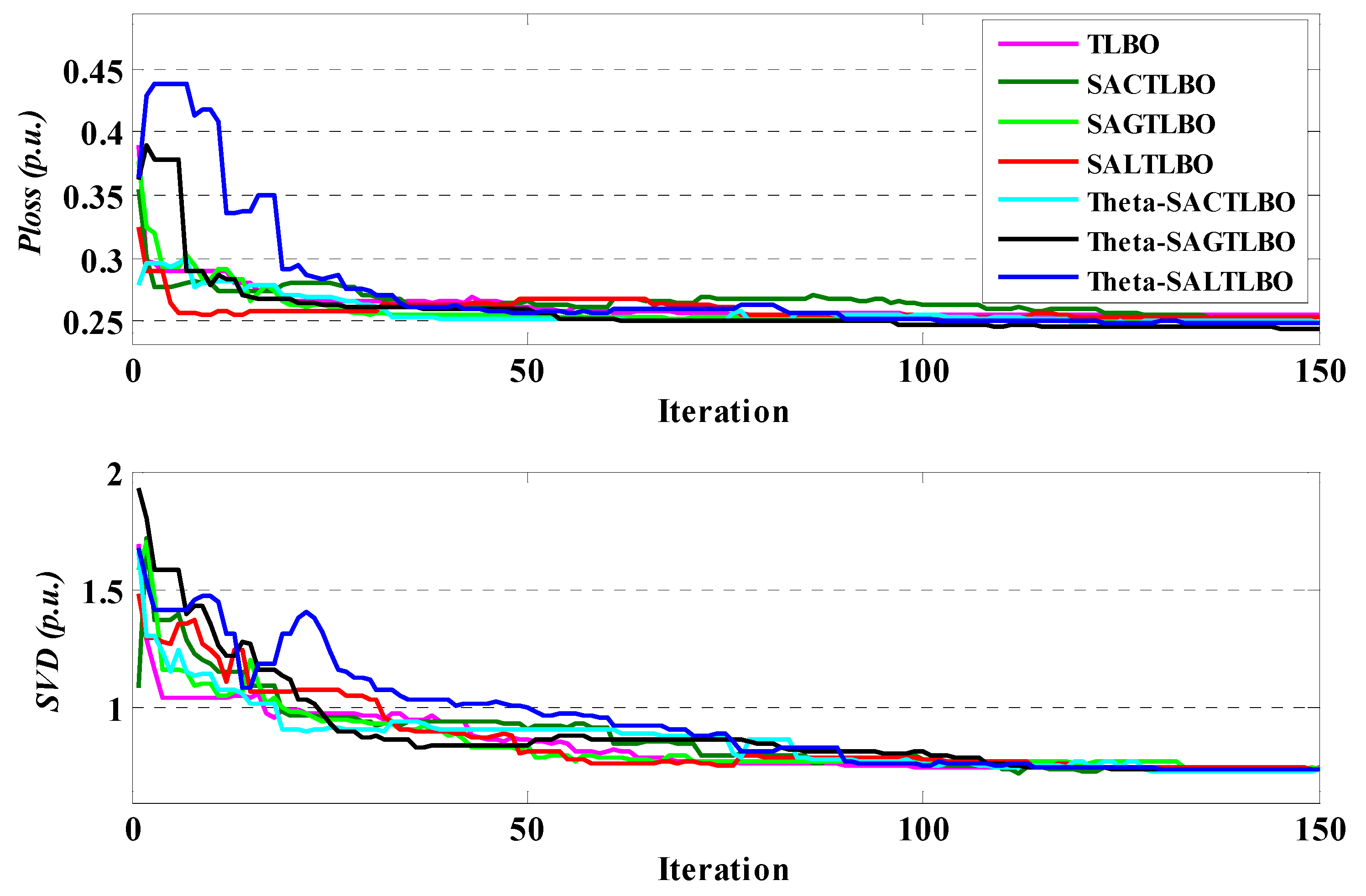
Rather than optimizing the SVD and active power losses separately in this work, both objective functions are optimized simultaneously utilizing the updated methods for this popular standard network. Table 10 summarizes the optimal control variables, SVD, and network losses obtained with previous and TLBO optimizers. The presented optimizers identified the optimal tradeoff solutions for active power losses and SVD. The optimal Volt-VAR control problem reveals that, in scenario 3 for this popular standard network, both SVD and power losses cannot be further decreased without the other deteriorating. The convergence characteristics for network loss minimization and SVD minimization are presented in Figure 12 for all TLBO optimizers.
In short, θ-SATLBO algorithms, as novel efficient optimization algorithms, confirmed their superior efficiency and reliability in finding the optimal solutions to several optimal Volt-VAR control issues over other well-known search approaches. Therefore, we can conclude that θ-SATLBO algorithms are suitable and powerful optimizers for optimizing real-world contemporary issues. Hence, those interested in other fields can effectively use this method in their field of work.
5. Conclusions
In this study, we enhanced the original TLBO method and present a θ-self-adaptive TLBO (θ-SATLBO) approach that incorporates the mutation operator into the habitat mutation. Additionally, new and effective mutation operators (i.e., Cauchy, Gaussian, and Lévy mutations) that are frequently employed in evolutionary algorithms were selected to increase the exploration potential and variety of the population in the improved θ-SATLBO technique. The proposed algorithms were run on IEEE 30- and IEEE 57-bus networks, and the resulting data were compared to those from the references. The simulation findings demonstrate that θ-SAGTLBO algorithms are more efficient than the other algorithms tested in this study at balancing global search capabilities to solve optimal Volt-VAR control issues. This study demonstrates that the provided algorithms can solve optimal Volt-VAR control issues due to their superior performance with various goal functions.
θ-SATLBO’s best optimized outcomes are better than those obtained by the other studied optimization algorithms. The efficient convergence of the real-parameter θ-SATLBO algorithms is demonstrated by their rapid convergence speed. It would be fascinating to apply real-parameter θ-SATLBO optimizers to engineering and science optimization problems in the future. It would also be beneficial to study the influence of different spirals on the real-parameter θ-SATLBO algorithms’ efficiency. In addition, statistical results from the perspective of standard deviations showed that the proposed algorithm was reasonably reliable compared to other comparative algorithms. However, for practical and real-time applications, further improvements in convergence speed and CPU time may be required.
Funding
This research received no external funding.
Institutional Review Board Statement
Not applicable.
Informed Consent Statement
Not applicable.
Data Availability Statement
Not applicable.
Conflicts of Interest
The author declare no conflict of interest.
References
- Rojas, D.G.; Lezama, J.L.; Villa, W. Metaheuristic Techniques Applied to the Optimal Reactive Power Dispatch: A Review. IEEE Lat. Am. Trans. 2016, 14, 2253–2263. [Google Scholar] [CrossRef]
- Naderi, E.; Narimani, H.; Fathi, M.; Narimani, M.R. A Novel Fuzzy Adaptive Configuration of Particle Swarm Optimization to Solve Large-Scale Optimal Reactive Power Dispatch. Appl. Soft Comput. 2017, 53, 441–456. [Google Scholar] [CrossRef]
- Ghasemi, M.; Ghavidel, S.; Ghanbarian, M.M.; Habibi, A. A New Hybrid Algorithm for Optimal Reactive Power Dispatch Problem with Discrete and Continuous Control Variables. Appl. Soft Comput. 2014, 22, 126–140. [Google Scholar] [CrossRef]
- Ghasemi, M.; Ghanbarian, M.M.; Ghavidel, S.; Rahmani, S.; Moghaddam, E.M. Modified Teaching Learning Algorithm and Double Differential Evolution Algorithm for Optimal Reactive Power Dispatch Problem: A Comparative Study. Inf. Sci. 2014, 278, 231–249. [Google Scholar] [CrossRef]
- Khazali, A.H.; Kalantar, M. Optimal Reactive Power Dispatch Based on Harmony Search Algorithm. Int. J. Electr. Power Energy Syst. 2011, 33, 684–692. [Google Scholar] [CrossRef]
- Roy, P.K.; Ghoshal, S.P.; Thakur, S.S. Optimal Var Control for Improvements in Voltage Profiles and for Real Power Loss Minimization Using Biogeography Based Optimization. Int. J. Electr. Power Energy Syst. 2012, 43, 830–838. [Google Scholar] [CrossRef]
- Zhang, X.; Chen, W.; Dai, C.; Cai, W. Dynamic Multi-Group Self-Adaptive Differential Evolution Algorithm for Reactive Power Optimization. Int. J. Electr. Power Energy Syst. 2010, 32, 351–357. [Google Scholar] [CrossRef]
- Zhao, B.; Guo, C.X.; Cao, Y.J. A Multiagent-Based Particle Swarm Optimization Approach for Optimal Reactive Power Dispatch. IEEE Trans. Power Syst. 2005, 20, 1070–1078. [Google Scholar] [CrossRef]
- Zhang, W.; Liu, Y. Multi-Objective Reactive Power and Voltage Control Based on Fuzzy Optimization Strategy and Fuzzy Adaptive Particle Swarm. Int. J. Electr. Power Energy Syst. 2008, 30, 525–532. [Google Scholar] [CrossRef]
- Abou El Ela, A.A.; Abido, M.A.; Spea, S.R. Differential Evolution Algorithm for Optimal Reactive Power Dispatch. Electr. Power Syst. Res. 2011, 81, 458–464. [Google Scholar] [CrossRef]
- Mahadevan, K.; Kannan, P.S. Comprehensive Learning Particle Swarm Optimization for Reactive Power Dispatch. Appl. Soft Comput. 2010, 10, 641–652. [Google Scholar] [CrossRef]
- Dai, C.; Chen, W.; Zhu, Y.; Zhang, X. Seeker Optimization Algorithm for Optimal Reactive Power Dispatch. IEEE Trans. Power Syst. 2009, 24, 1218–1231. [Google Scholar]
- Xu, Y.; Zhang, W.; Liu, W.; Ferrese, F. Multiagent-Based Reinforcement Learning for Optimal Reactive Power Dispatch. IEEE Trans. Syst. Man Cybern. Part C 2012, 42, 1742–1751. [Google Scholar] [CrossRef]
- Mandal, B.; Roy, P.K. Optimal Reactive Power Dispatch Using Quasi-Oppositional Teaching Learning Based Optimization. Int. J. Electr. Power Energy Syst. 2013, 53, 123–134. [Google Scholar] [CrossRef]
- Rao, R.V.; Savsani, V.J.; Vakharia, D.P. Teaching–Learning-Based Optimization: A Novel Method for Constrained Mechanical Design Optimization Problems. Comput. Des. 2011, 43, 303–315. [Google Scholar] [CrossRef]
- Chen, G.; Liu, L.; Song, P.; Du, Y. Chaotic Improved PSO-Based Multi-Objective Optimization for Minimization of Power Losses and L Index in Power Systems. Energy Convers. Manag. 2014, 86, 548–560. [Google Scholar] [CrossRef]
- Shaheen, A.M.; Spea, S.R.; Farrag, S.M.; Abido, M.A. A Review of Meta-Heuristic Algorithms for Reactive Power Planning Problem. Ain Shams Eng. J. 2018, 9, 215–231. [Google Scholar] [CrossRef] [Green Version]
- Naderi, E.; Pourakbari-Kasmaei, M.; Abdi, H. An Efficient Particle Swarm Optimization Algorithm to Solve Optimal Power Flow Problem Integrated with FACTS Devices. Appl. Soft Comput. 2019, 80, 243–262. [Google Scholar] [CrossRef]
- Vadivelu, K.R.; Marutheswar, G. V Soft Computing Technique Based Reactive Power Planning Using NVSI. J. Electr. Syst. 2015, 11, 89–101. [Google Scholar]
- Dutta, S.; Roy, P.K.; Nandi, D. Optimal Location of STATCOM Using Chemical Reaction Optimization for Reactive Power Dispatch Problem. Ain Shams Eng. J. 2016, 7, 233–247. [Google Scholar] [CrossRef] [Green Version]
- Ghasemi, M.; Taghizadeh, M.; Ghavidel, S.; Aghaei, J.; Abbasian, A. Solving Optimal Reactive Power Dispatch Problem Using a Novel Teaching–Learning-Based Optimization Algorithm. Eng. Appl. Artif. Intell. 2015, 39, 100–108. [Google Scholar] [CrossRef]
- Lenin, K.; Reddy, B.R.; Kalavathi, M.S. Water Cycle Algorithm for Solving Optimal Reactive Power Dispatch Problem. J. Eng. Technol. Res. 2014, 2, 1–11. [Google Scholar]
- Mei, R.N.S.; Sulaiman, M.H.; Mustaffa, Z.; Daniyal, H. Optimal Reactive Power Dispatch Solution by Loss Minimization Using Moth-Flame Optimization Technique. Appl. Soft Comput. 2017, 59, 210–222. [Google Scholar]
- Nguyen, T.T.; Vo, D.N. Improved Social Spider Optimization Algorithm for Optimal Reactive Power Dispatch Problem with Different Objectives. Neural Comput. Appl. 2020, 32, 5919–5950. [Google Scholar] [CrossRef]
- Davoodi, E.; Babaei, E.; Mohammadi-Ivatloo, B.; Rasouli, M. A Novel Fast Semidefinite Programming-Based Approach for Optimal Reactive Power Dispatch. IEEE Trans. Ind. Inform. 2019, 16, 288–298. [Google Scholar] [CrossRef]
- Sulaiman, M.H.; Mustaffa, Z.; Mohamed, M.R.; Aliman, O. Using the Gray Wolf Optimizer for Solving Optimal Reactive Power Dispatch Problem. Appl. Soft Comput. 2015, 32, 286–292. [Google Scholar] [CrossRef] [Green Version]
- Bingane, C.; Anjos, M.F.; Le Digabel, S. Tight-and-Cheap Conic Relaxation for the Optimal Reactive Power Dispatch Problem. IEEE Trans. Power Syst. 2019, 34, 4684–4693. [Google Scholar] [CrossRef]
- Polprasert, J.; Ongsakul, W.; Dieu, V.N. Optimal Reactive Power Dispatch Using Improved Pseudo-Gradient Search Particle Swarm Optimization. Electr. Power Compon. Syst. 2016, 44, 518–532. [Google Scholar] [CrossRef]
- Vo, D.N.; Nguyen, T.P.; Nguyen, K.D. Multi-Objective Security Constrained Optimal Active and Reactive Power Dispatch Using Hybrid Particle Swarm Optimization and Differential Evolution. GMSARN Int. J. 2018, 12, 84–117. [Google Scholar]
- Mehdinejad, M.; Mohammadi-Ivatloo, B.; Dadashzadeh-Bonab, R.; Zare, K. Solution of Optimal Reactive Power Dispatch of Power Systems Using Hybrid Particle Swarm Optimization and Imperialist Competitive Algorithms. Int. J. Electr. Power Energy Syst. 2016, 83, 104–116. [Google Scholar] [CrossRef]
- Li, Y.; Li, X.; Li, Z. Reactive Power Optimization Using Hybrid CABC-DE Algorithm. Electr. Power Compon. Syst. 2017, 45, 980–989. [Google Scholar] [CrossRef]
- Chen, G.; Liu, L.; Zhang, Z.; Huang, S. Optimal Reactive Power Dispatch by Improved GSA-Based Algorithm with the Novel Strategies to Handle Constraints. Appl. Soft Comput. 2017, 50, 58–70. [Google Scholar] [CrossRef]
- Rayudu, K.; Yesuratnam, G.; Jayalaxmi, A. Ant Colony Optimization Algorithm Based Optimal Reactive Power Dispatch to Improve Voltage Stability. In Proceedings of the 2017 International Conference on Circuit, Power and Computing Technologies (ICCPCT), Kollam, India, 20–21 April 2017; pp. 1–6. [Google Scholar]
- Nguyen, T.T.; Vo, D.N.; Van Tran, H.; Van Dai, L. Optimal Dispatch of Reactive Power Using Modified Stochastic Fractal Search Algorithm. Complexity 2019, 2019, 4670820. [Google Scholar] [CrossRef]
- Li, Z.; Cao, Y.; Van Dai, L.; Yang, X.; Nguyen, T.T. Finding Solutions for Optimal Reactive Power Dispatch Problem by a Novel Improved Antlion Optimization Algorithm. Energies 2019, 12, 2968. [Google Scholar] [CrossRef] [Green Version]
- ben oualid Medani, K.; Sayah, S.; Bekrar, A. Whale Optimization Algorithm Based Optimal Reactive Power Dispatch: A Case Study of the Algerian Power System. Electr. Power Syst. Res. 2018, 163, 696–705. [Google Scholar] [CrossRef]
- Yalcin, E.; TAPLAMACIOĞLU, M.C.; Ertuğrul, Ç.A.M. The Adaptive Chaotic Symbiotic Organisms Search Algorithm Proposal for Optimal Reactive Power Dispatch Problem in Power Systems. Electrica 2019, 19, 37–47. [Google Scholar] [CrossRef] [Green Version]
- Radosavljević, J.; Jevtić, M.; Milovanović, M. A Solution to the ORPD Problem and Critical Analysis of the Results. Electr. Eng. 2018, 100, 253–265. [Google Scholar] [CrossRef]
- Heidari, A.A.; Abbaspour, R.A.; Jordehi, A.R. Gaussian Bare-Bones Water Cycle Algorithm for Optimal Reactive Power Dispatch in Electrical Power Systems. Appl. Soft Comput. 2017, 57, 657–671. [Google Scholar] [CrossRef]
- Muhammad, Y.; Khan, R.; Ullah, F.; Aslam, M.S.; Raja, M.A.Z. Design of Fractional Swarming Strategy for Solution of Optimal Reactive Power Dispatch. Neural Comput. Appl. 2020, 32, 10501–10518. [Google Scholar] [CrossRef]
- Rajan, A.; Malakar, T. Exchange Market Algorithm Based Optimum Reactive Power Dispatch. Appl. Soft Comput. 2016, 43, 320–336. [Google Scholar] [CrossRef]
- Abaci, K.; Yamaçli, V. Optimal Reactive-Power Dispatch Using Differential Search Algorithm. Electr. Eng. 2017, 99, 213–225. [Google Scholar] [CrossRef]
- Mouassa, S.; Bouktir, T.; Salhi, A. Ant Lion Optimizer for Solving Optimal Reactive Power Dispatch Problem in Power Systems. Eng. Sci. Technol. Int. J. 2017, 20, 885–895. [Google Scholar] [CrossRef]
- Anbarasan, P.; Jayabarathi, T. Optimal Reactive Power Dispatch Problem Solved by an Improved Colliding Bodies Optimization Algorithm. In Proceedings of the 2017 IEEE International Conference on Environment and Electrical Engineering and 2017 IEEE Industrial and Commercial Power Systems Europe (EEEIC/I&CPS Europe), Milan, Italy, 6–9 June 2017; pp. 1–6. [Google Scholar]
- Barakat, A.F.; El-Sehiemy, R.; Elsaid, M.; Osman, E. Solving Reactive Power Dispatch Problem by Using JAYA Optimization Algorithm. In Proceedings of the International Journal of Engineering Research in Africa; Trans Tech Publications, Ltd.: Freienbach, Switzerland, 2018; Volume 36, pp. 12–24. [Google Scholar]
- Nuaekaew, K.; Artrit, P.; Pholdee, N.; Bureerat, S. Optimal Reactive Power Dispatch Problem Using a Two-Archive Multi-Objective Grey Wolf Optimizer. Expert Syst. Appl. 2017, 87, 79–89. [Google Scholar] [CrossRef]
- Shareef, S.K.M.; Rao, R.S. Optimal Reactive Power Dispatch under Unbalanced Conditions Using Hybrid Swarm Intelligence. Comput. Electr. Eng. 2018, 69, 183–193. [Google Scholar] [CrossRef]
- Meddeb, A.; Amor, N.; Abbes, M.; Chebbi, S. A Novel Approach Based on Crow Search Algorithm for Solving Reactive Power Dispatch Problem. Energies 2018, 11, 3321. [Google Scholar] [CrossRef] [Green Version]
- Martinez-Rojas, M.; Sumper, A.; Gomis-Bellmunt, O.; Sudrià-Andreu, A. Reactive Power Dispatch in Wind Farms Using Particle Swarm Optimization Technique and Feasible Solutions Search. Appl. Energy 2011, 88, 4678–4686. [Google Scholar] [CrossRef]
- Subbaraj, P.; Rajnarayanan, P.N. Optimal Reactive Power Dispatch Using Self-Adaptive Real Coded Genetic Algorithm. Electr. Power Syst. Res. 2009, 79, 374–381. [Google Scholar] [CrossRef]
- Ramirez, J.M.; Gonzalez, J.M.; Ruben, T.O. An Investigation about the Impact of the Optimal Reactive Power Dispatch Solved by DE. Int. J. Electr. Power Energy Syst. 2011, 33, 236–244. [Google Scholar] [CrossRef]
- Feller, W. An Introduction to Probability Theory and Its Applications; John Wiley & Sons: Hoboken, NJ, USA, 2008; Volume 2, ISBN 8126518065. [Google Scholar]
- Kolmogorov, A.N.; Gnedenko, B.V. Limit Distributions for Sums of Independent Random Variables; Addison-Wesley: Boston, MA, USA, 1968. [Google Scholar]
- Lee, C.-Y.; Yao, X. Evolutionary Programming Using Mutations Based on the Lévy Probability Distribution. IEEE Trans. Evol. Comput. 2004, 8, 1–13. [Google Scholar] [CrossRef] [Green Version]
- Abdi, H.; Moradi, M.; Asadi, R.; Naderi, S.; Amirian, B.; Karimi, F. Optimal Reactive Power Dispatch Problem: A Comprehensive Study on Meta-Heuristic Algorithms. J. Energy Manag. Technol. 2021, 5, 67–77. [Google Scholar]
- Ghasemi, M.; Ghavidel, S.; Ghanbarian, M.M.; Gitizadeh, M. Multi-Objective Optimal Electric Power Planning in the Power System Using Gaussian Bare-Bones Imperialist Competitive Algorithm. Inf. Sci. 2015, 294, 286–304. [Google Scholar] [CrossRef]
- Kien, L.C.; Hien, C.T.; Nguyen, T.T. Optimal Reactive Power Generation for Transmission Power Systems Considering Discrete Values of Capacitors and Tap Changers. Appl. Sci. 2021, 11, 5378. [Google Scholar] [CrossRef]
- Ghasemi, M. Modified Imperialist Competitive Algorithm for Optimal Reactive Power Dispatch. Int. J. Electr. Electron. Sci. 2017, 4, 1–15. [Google Scholar]
- Shaheen, A.M.; El-Sehiemy, R.A.; Farrag, S.M. Integrated Strategies of Backtracking Search Optimizer for Solving Reactive Power Dispatch Problem. IEEE Syst. J. 2016, 12, 424–433. [Google Scholar] [CrossRef]
Figure 1.
Flow chart showing the operation of the proposed optimizers.

Figure 2.
The diagram of the IEEE 30-bus network (system 1).

Figure 3.
Performance characteristics of TLBO optimizers for case 1 of system 1.

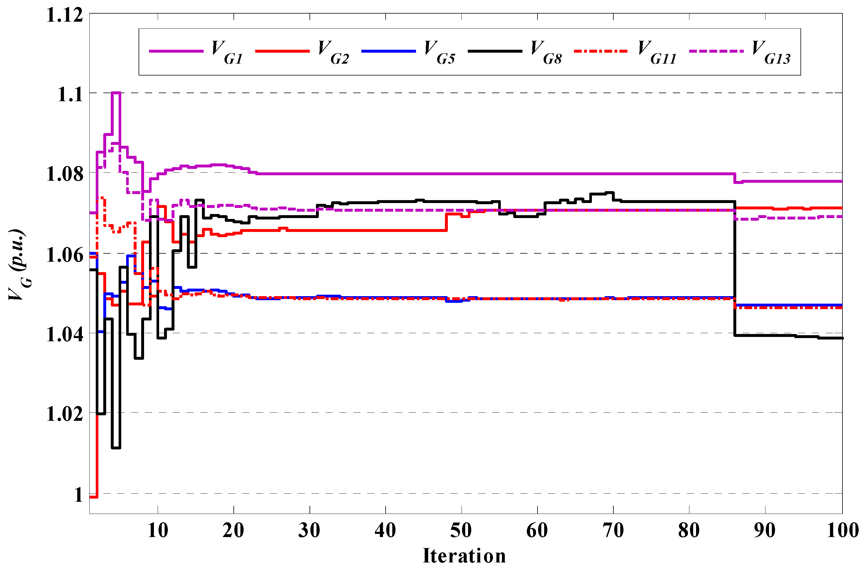
Figure 4.
Convergence of VG for case 1 using θ-SAGTLBO of system 1.

Figure 5.
Convergence of T for case 1 using θ-SAGTLBO of system 1.

Figure 6.
Convergence of QC for case 1 using θ-SAGTLBO of system 1.

Figure 7.
Performance characteristics of TLBO optimizers for case 2 of system 1.

Figure 8.
Performance characteristics of TLBO optimizers for case 3 of system 1.

Figure 9.
The diagram of the IEEE 57-bus network (system 2).

Figure 10.
Performance characteristics of TLBO optimizers for case 1 of system 2.

Figure 11.
Performance characteristics of TLBO optimizers for case 2 of system 2.

Figure 12.
Performance characteristics of TLBO optimizers for case 3 of system 2.


Table 1.
The basic data of IEEE 30-bus network in p.u. (system 1) [21].
Table 1.
The basic data of IEEE 30-bus network in p.u. (system 1) [21].
| Units Reactive Power | |||||||||||
| Bus | 1 | 2 | 5 | 8 | 11 | 13 | |||||
| 0.596 | 0.48 | 0.6 | 0.53 | 0.15 | 0.155 | ||||||
| −0.298 | −0.24 | −0.3 | −0.265 | −0.075 | −0.078 | ||||||
| Voltage and tap setting | |||||||||||
| 1.1 | 0.9 | 1.05 | 0.95 | 1.05 | 0.95 | ||||||
| Reactive power parallel compensators | |||||||||||
| Bus | 3 | 10 | 24 | ||||||||
| 0.36 | 0.36 | 0.36 | |||||||||
| −0.12 | −0.12 | −0.12 | |||||||||
Table 2.
Best optimal parameter settings in p.u. for case 1 of system 1.
| Variable | θ-SAGTLBO |
|---|---|
| VG1 | 1.078 |
| VG2 | 1.0689 |
| VG5 | 1.0464 |
| VG8 | 1.0468 |
| VG11 | 1.0385 |
| VG13 | 1.0711 |
| T6–9 | 1.05 |
| T6–10 | 0.97 |
| T4–12 | 1.0 |
| T28–27 | 0.97 |
| QC3 | −0.04 |
| QC10 | 0.34 |
| QC24 | 0.11 |
| Ploss | 0.0486217 |
| SVD | 0.9455 |
Table 3.
Statistical details for case 1 of system 1.
| Algorithms | Mean (p.u.) | Worst (p.u.) | Best (p.u.) | Time (sec) | %Psave | Std. |
|---|---|---|---|---|---|---|
| DE [4] | 0.049981 | 0.05241 | 0.049121 | 25.25 | 17.97 | 8.783 × 10⁻³ |
| PBIL [4] | 0.049405 | 0.049615 | 0.049144 | 18.72 | 17.93 | 1.662 × 10⁻⁴ |
| BB–BC [4] | 0.049426 | 0.049708 | 0.04908 | 19.14 | 18.03 | 8.009 × 10⁻⁴ |
| BRCFF [4] | 0.049118 | 0.049391 | 0.049059 | 15.67 | 18.07 | 9.447 × 10⁻⁵ |
| CSS [4] | 0.049552 | 0.050673 | 0.049062 | 21.00 | 18.06 | 7.114 × 10⁻³ |
| LCA [4] | 0.049621 | 0.050086 | 0.049092 | 21.02 | 18.01 | 4.478 × 10⁻³ |
| ABC [4] | 0.049338 | 0.04972 | 0.049064 | 20.87 | 18.06 | 6.605 × 10⁻⁴ |
| DE/best/2 [4] | 0.049492 | 0.051064 | 0.049073 | 23.55 | 18.05 | 8.488 × 10⁻⁴ |
| ACOR [4] | 0.049587 | 0.051963 | 0.049147 | 21.62 | 17.92 | 3.197 × 10⁻³ |
| HSA [5] | 0.04924 | 0.049653 | 0.049059 | N.A. | 17.32 | N.A. |
| PSO [5] | 0.04972 | 0.050576 | 0.049239 | N.A. | 17.02 | N.A. |
| SGA [5] | 0.050378 | 0.051651 | 0.049408 | N.A. | 16.07 | N.A. |
| IWO [3] | 0.05234 | 0.05456 | 0.049344 | 71.54 | 17.59 | 7.587 × 10⁻² |
| GBTLBO [20] | 0.048686 | 0.048688 | 0.048685 | 37.24 | 18.69 | 2.33 × 10⁻⁵ |
| BBDE [20] | 0.049016 | 0.049019 | 0.049015 | 33.62 | 18.14 | 3.48 × 10⁻⁵ |
| BBPSO [20] | 0.048924 | 0.048927 | 0.048922 | 35.55 | 18.30 | 6.01 × 10⁻⁵ |
| CLPSO [7] | 0.049453 | N.A. | 0.049292 | 128.7073 | 18.2689 | 1.14 × 10⁻⁴ |
| AGA [7] | 0.051067 | N.A. | 0.04971 | 147.563 | 17.5759 | 1.074 × 10⁻³ |
| DE [7] | 0.049443 | N.A. | 0.049338 | 141.3891 | 18.1918 | 6.6 × 10⁻⁵ |
| PSO-w [7] | 0.049516 | N.A. | 0.049232 | 143.499 | 18.3684 | 5.62 × 10⁻⁴ |
| PSO-cf [7] | 0.049378 | N.A. | 0.049228 | 144.3448 | 18.3751 | 1.71 × 10⁻⁴ |
| DMSDE [7] | 0.049242 | N.A. | 0.04922 | 143.88 | 18.3883 | 1.7 × 10⁻⁵ |
| MAPSO [8] | 0.048751 | 0.048759 | 0.048747 | 41.93 | 18.59 | N.A. |
| PSO [8] | 0.049973 | 0.050769 | 0.049262 | 59.21 | 17.62 | N.A. |
| SGA [8] | 0.05081 | 0.05214 | 0.0498 | 156.34 | 16.84 | N.A. |
| MGBICA [55] | N.A. | N.A. | 0.04937 | N.A. | N.A. | N.A. |
| GBICA [55] | N.A. | N.A. | 0.05044 | N.A. | N.A. | N.A. |
| GDE3 [55] | N.A. | N.A. | 0.050251 | N.A. | N.A. | N.A. |
| NKEA [55] | N.A. | N.A. | 0.050289 | N.A. | N.A. | N.A. |
| iTDEA [55] | N.A. | N.A. | 0.050354 | N.A. | N.A. | N.A. |
| MOPSO-CD [55] | N.A. | N.A. | 0.05013 | N.A. | N.A. | N.A. |
| VEPSO [55] | N.A. | N.A. | 0.050378 | N.A. | N.A. | N.A. |
| OMOPSO [55] | N.A. | N.A. | 0.050164 | N.A. | N.A. | N.A. |
| NSGA-II [55] | N.A. | N.A. | 0.050564 | N.A. | N.A. | N.A. |
| JGGA [55] | N.A. | N.A. | 0.049789 | N.A. | N.A. | N.A. |
| TLBO | 0.049282 | 0.0492647 | 0.0491293 | 19.61 | 17.95 | 7.29 × 10⁻³ |
| SACTLBO | 0.0491529 | 0.0491853 | 0.0490154 | 20.93 | 18.14 | 8.917 × 10⁻⁴ |
| SAGTLBO | 0.0488227 | 0.0490145 | 0.048699 | 21.25 | 18.67 | 2.066 × 10⁻⁴ |
| SALTLBO | 0.0491007 | 0.0491127 | 0.0489984 | 21.31 | 18.17 | 5.783 × 10⁻⁴ |
| θ-SACTLBO | 0.0486309 | 0.0486468 | 0.0486244 | 20.16 | 18.79 | 1.507 × 10⁻⁵ |
| θ-SAGTLBO | 0.0486237 | 0.0486325 | 0.0486217 | 20.18 | 18.81 | 0.163 × 10⁻⁵ |
| θ-SALTLBO | 0.04865 | 0.0486618 | 0.048638 | 20.19 | 18.77 | 3.044 × 10⁻⁵ |
N.A.: Not available.
Table 4.
Best optimal parameters settings for case 2 of system 1.
| Variable | Algorithms | |
|---|---|---|
| θ-SACTLBO | θ-SAGTLBO | |
| VG1 | 1.0209 | 1.0206 |
| VG2 | 1.0248 | 1.0254 |
| VG5 | 1.0174 | 1.0174 |
| VG8 | 1.0074 | 1.0072 |
| VG11 | 1.0043 | 1.0043 |
| VG13 | 1.024 | 1.0242 |
| T6–9 | 1.02 | 1.02 |
| T6–10 | 0.95 | 0.95 |
| T4–12 | 0.97 | 0.97 |
| T28–27 | 0.95 | 0.95 |
| QC3 | −0.12 | −0.12 |
| QC10 | 0.2 | 0.2 |
| QC24 | 0.12 | 0.12 |
| Ploss | 0.0567107 | 0.0568303 |
| SVD | 0.1233 | 0.1233 |
Table 5.
Statistical details for case 2 of system 1.
| Algorithms | Mean (p.u.) | Worst (p.u.) | Best (p.u.) | Time (s) | Std. |
|---|---|---|---|---|---|
| HSA [5] | 0.1443 | 0.1589 | 0.1349 | N.A. | N.A. |
| PSO [5] | 0.1449 | 0.1639 | 0.1424 | N.A. | N.A. |
| SGA [5] | 0.1523 | 0.1717 | 0.1501 | N.A. | N.A. |
| GWO [26] | 0.14484 | 0.17273 | 0.12604 | N.A. | N.A. |
| MGBICA [55] | N.A. | N.A. | 0.1239 | N.A. | N.A. |
| GBICA [55] | N.A. | N.A. | 0.132 | N.A. | N.A. |
| GDE3 [55] | N.A. | N.A. | 0.1357 | N.A. | N.A. |
| NKEA [55] | N.A. | N.A. | 0.1333 | N.A. | N.A. |
| iTDEA [55] | N.A. | N.A. | 0.1305 | N.A. | N.A. |
| MOPSO-CD [55] | N.A. | N.A. | 0.1335 | N.A. | N.A. |
| VEPSO [55] | N.A. | N.A. | 0.1308 | N.A. | N.A. |
| OMOPSO [55] | N.A. | N.A. | 0.1316 | N.A. | N.A. |
| NSGA-II [55] | N.A. | N.A. | 0.1344 | N.A. | N.A. |
| JGGA [55] | N.A. | N.A. | 0.1407 | N.A. | N.A. |
| SFOA [56] | 0.2326 | N.A. | 0.1588 | 6.9 | N.A. |
| SSA [56] | 0.3392 | N.A. | 0.1806 | 6.3 | N.A. |
| ABC [57] | 0.1367 | 0.138 | 0.1350 | N.A. | 8.89 × 10⁻⁵ |
| BFO [57] | 0.151 | 0.153 | 0.149 | N.A. | 8.90 × 10⁻⁵ |
| TLBO | 0.1402 | 0.1565 | 0.1278 | 22.25 | 9.825 × 10⁻⁴ |
| SACTLBO | 0.1378 | 0.141 | 0.1243 | 26.68 | 5.314 × 10⁻⁴ |
| SAGTLBO | 0.1318 | 0.1426 | 0.1236 | 27.15 | 3.404 × 10⁻⁴ |
| SALTLBO | 0.1327 | 0.1436 | 0.1242 | 27.41 | 3.169 × 10⁻⁴ |
| θ-SACTLBO | 0.1255 | 0.1305 | 0.1233 | 24.57 | 4.732 × 10⁻⁵ |
| θ-SAGTLBO | 0.1249 | 0.1263 | 0.1233 | 25.91 | 8.512 × 10⁻⁶ |
| θ-SALTLBO | 0.1251 | 0.1305 | 0.1234 | 25.48 | 3.905 × 10⁻⁵ |
Table 6.
Best optimal parameters settings for case 3 of system 1.
| Variable | Algorithms | ||||||
|---|---|---|---|---|---|---|---|
| TLBO | SACTLBO | SAGTLBO | SALTLBO | θ-SACTLBO | θ-SAGTLBO | θ-SALTLBO | |
| VG1 | 1.0706 | 1.0764 | 1.0745 | 1.0772 | 1.0772 | 1.0772 | 1.0771 |
| VG2 | 1.0593 | 1.067 | 1.0651 | 1.0679 | 1.0679 | 1.068 | 1.0679 |
| VG5 | 1.0416 | 1.0437 | 1.0414 | 1.0452 | 1.0451 | 1.0451 | 1.0451 |
| VG8 | 1.0467 | 1.0439 | 1.0415 | 1.0456 | 1.0456 | 1.0456 | 1.0455 |
| VG11 | 1.0443 | 1.0429 | 1.0413 | 1.043 | 0.9925 | 0.9924 | 0.9929 |
| VG13 | 1.0448 | 1.0395 | 1.0393 | 1.0397 | 1.0395 | 1.0395 | 1.0395 |
| T6–9 | 1.04 | 1.05 | 1.05 | 1.05 | 1.05 | 1.05 | 1.05 |
| T6–10 | 1.04 | 1.02 | 1.02 | 1.02 | 1.05 | 1.05 | 1.05 |
| T4–12 | 1.0 | 1.03 | 1.03 | 1.03 | 1.03 | 1.03 | 1.03 |
| T28–27 | 1.0 | 0.99 | 0.99 | 1.0 | 1.0 | 1.0 | 1.0 |
| QC3 | 0.06 | −0.03 | 0.0 | −0.04 | −0.04 | −0.04 | −0.04 |
| QC10 | 0.16 | 0.2 | 0.22 | 0.2 | 0.36 | 0.36 | 0.36 |
| QC24 | 0.16 | 0.11 | 0.11 | 0.11 | 0.12 | 0.12 | 0.12 |
| Ploss | 0.050151 | 0.0495614 | 0.0496281 | 0.0494799 | 0.0495136 | 0.0495125 | 0.0495157 |
| SVD | 0.4459 | 0.3845 | 0.3777 | 0.3916 | 0.3752 | 0.3752 | 0.3754 |
Table 7.
The limits of the control variables for the IEEE 57-bus network in p.u. (system 2) [21].
Table 7.
The limits of the control variables for the IEEE 57-bus network in p.u. (system 2) [21].
| Limits of Generation Reactive Power | |||||||||||
| Bus | 1 | 2 | 3 | 6 | 8 | 9 | 12 | ||||
| 1.5 | 0.5 | 0.6 | 0.25 | 2.0 | 0.09 | 1.55 | |||||
| −0.2 | −0.17 | −0.1 | −0.08 | −1.4 | −0.03 | −1.5 | |||||
| Limits of voltage and tap setting | |||||||||||
| 1.06 | 0.94 | 1.06 | 0.94 | 1.1 | 0.9 | ||||||
| Limits of reactive power sources | |||||||||||
| Bus | 18 | 25 | 53 | ||||||||
| 0.1 | 0.059 | 0.063 | |||||||||
| 0.0 | 0.0 | 0.0 | |||||||||
Table 8.
Statistical details for case 1 of system 2.
| Algorithms | Mean (p.u.) | Worst (p.u.) | Best (p.u.) | Time (s) | %Psave | Std. |
|---|---|---|---|---|---|---|
| MICA [58] | 0.2426758 | 0.2429263 | 0.2425668 | 49.28 | 14.7752 | 2.8859 × 10⁻⁵ |
| ICA [58] | 0.2538722 | 0.2554803 | 0.244799 | 44.32 | 13.9909 | 8.0561 × 10⁻³ |
| HSA [5] | 0.25924 | 0.269653 | 0.249059 | N.A. | N.A. | N.A. |
| PSO [5] | 0.264742 | 0.270576 | 0.2503 | N.A. | N.A. | N.A. |
| SGA [5] | 0.268378 | 0.277651 | 0.2564 | N.A. | N.A. | N.A. |
| CGA [7] | 0.264826 | N.A. | 0.248853 | 176.6708 | 12.5666 | 6.671 × 10⁻³ |
| DE [7] | 0.255509 | N.A. | 0.250862 | 152.0557 | 11.8607 | 3.003 × 10⁻³ |
| PSO-w [7] | 0.274727 | N.A. | 0.2440741 | 155.4432 | 14.2456 | 4.9692 × 10⁻² |
| DMSDE [7] | 0.24359 | N.A. | 0.24266 | 156.11 | 14.7425 | 1.011 × 10⁻³ |
| PSO-cf [7] | 0.263949 | N.A. | 0.243449 | 152.7011 | 14.4653 | 2.6513 × 10⁻² |
| AGA [7] | 0.253251 | N.A. | 0.244857 | 165.8703 | 13.9706 | 6.635 × 10⁻³ |
| CLPSO [7] | 0.256381 | N.A. | 0.250684 | 104.4016 | 11.9233 | 3.601 × 10⁻³ |
| SOA [12] | 0.2427078 | 0.2428046 | 0.2426548 | 391.32 | 14.7443 | 4.2081 × 10⁻⁵ |
| L-SACP-DE [12] | 0.310326 | 0.3697873 | 0.2791553 | 428.98 | 1.92 | 3.2232 × 10⁻² |
| PSO-cf [12] | 0.2469805 | 0.2603275 | 0.2428022 | 408.19 | 14.6925 | 6.6294 × 10⁻³ |
| SPSO-07 [12] | 0.2475227 | 0.2545745 | 0.2443043 | 137.35 | 14.1647 | 2.833 × 10⁻³ |
| AGA [12] | 0.2512784 | 0.2676169 | 0.2456484 | 449.28 | 13.6925 | 6.0068 × 10⁻³ |
| PSO-w [12] | 0.2472596 | 0.2615279 | 0.2427052 | 408.48 | 14.7266 | 7.0143 × 10⁻³ |
| L-DE [12] | 0.3317783 | 0.4190941 | 0.2781264 | 431.41 | 2.2815 | 4.7072 × 10⁻² |
| CLPSO [12] | 0.2467307 | 0.2478083 | 0.245152 | 426.85 | 13.8669 | 9.3415 × 10⁻⁴ |
| L-SaDE [12] | 0.2431129 | 0.2439142 | 0.2426739 | 410.14 | 14.7376 | 4.8156 × 10⁻⁴ |
| CGA [12] | 0.2629356 | 0.2750772 | 0.2524411 | 411.38 | 11.3059 | 6.2951 × 10⁻³ |
| PSO–ICA [30] | N.A. | N.A. | 0.241386 | 1450 | N.A. | N.A. |
| ICA [30] | N.A. | N.A. | 0.241607 | 1018 | N.A. | N.A. |
| PSO [30] | N.A. | N.A. | 0.247742 | 927 | N.A. | N.A. |
| MGBICA [30] | N.A. | N.A. | 0.248863 | N.A. | N.A. | N.A. |
| GBICA [56] | N.A. | N.A. | 0.249666 | N.A. | N.A. | N.A. |
| GDE3 [56] | N.A. | N.A. | 0.250946 | N.A. | N.A. | N.A. |
| NKEA [56] | N.A. | N.A. | 0.250113 | N.A. | N.A. | N.A. |
| iTDEA [56] | N.A. | N.A. | 0.24938 | N.A. | N.A. | N.A. |
| MOPSO-CD [56] | N.A. | N.A. | 0.248914 | N.A. | N.A. | N.A. |
| VEPSO [56] | N.A. | N.A. | 0.248955 | N.A. | N.A. | N.A. |
| OMOPSO [56] | N.A. | N.A. | 0.252417 | N.A. | N.A. | N.A. |
| NSGA-II [56] | N.A. | N.A. | 0.252599 | N.A. | N.A. | N.A. |
| JGGA [56] | N.A. | N.A. | 0.249124 | N.A. | N.A. | N.A. |
| COA [58] | 0.268983 | N.A. | 0.245358 | 23.2 | N.A. | N.A. |
| SFOA [58] | 0.284249 | N.A. | 0.266541 | 21.3 | N.A. | N.A. |
| SSA [58] | 0.270306 | N.A. | 0.253854 | 21.8 | N.A. | N.A. |
| WCA [58] | 0.265319 | N.A. | 0.260402 | 27.4 | N.A. | N.A. |
| SCA [55] | N.A. | N.A. | 0.2540635 | N.A. | N.A. | N.A. |
| HGWO-PSO [55] | N.A. | N.A. | 0.2391005 | N.A. | N.A. | N.A. |
| BSO-5 [59] | 0.2509 | 0.2569 | 0.24640 | N.A. | N.A. | 2.64 × 10⁻³ |
| BSO-4 [59] | 0.248382 | 0.25398 | 0.243744 | N.A. | N.A. | 2.96 × 10⁻³ |
| BSO-3 [59] | 0.24944 | 0.260097 | 0.244492 | N.A. | N.A. | 3.32 × 10⁻³ |
| BSO-2 [59] | 0.249935 | 0.256244 | 0.244856 | N.A. | N.A. | 2.76 × 10⁻³ |
| BSO-1 [59] | 0.25099 | 0.26265 | 0.24536 | N.A. | N.A. | 3.75 × 10⁻³ |
| TLBO | 0.2469017 | 0.2472561 | 0.2465887 | 41.62 | 13.36 | 8.45 × 10⁻³ |
| SACTLBO | 0.2425682 | 0.2427194 | 0.2424759 | 45.35 | 14.81 | 5.708 × 10⁻⁴ |
| SAGTLBO | 0.2424794 | 0.242508 | 0.2422971 | 45.06 | 14.87 | 4.915 × 10⁻⁴ |
| SALTLBO | 0.2426853 | 0.2428917 | 0.2424638 | 44.94 | 14.81 | 5.055 × 10⁻⁴ |
| θ-SACTLBO | 0.241685 | 0.241711 | 0.241473 | 42.25 | 15.16 | 2.748 × 10⁻⁴ |
| θ-SAGTLBO | 0.2373008 | 0.2373965 | 0.2372619 | 42.78 | 16.64 | 1.381 × 10⁻⁵ |
| θ-SALTLBO | 0.2403196 | 0.2404745 | 0.2402684 | 43.17 | 15.58 | 9.254 × 10⁻⁵ |
Table 9.
Statistical details for case 2 of system 2.
| Algorithms | Mean (p.u.) | Worst (p.u.) | Best (p.u.) | Times (s) | Std. |
|---|---|---|---|---|---|
| PSO–ICA [30] | N.A. | N.A. | 0.6829 | N.A. | N.A. |
| ICA [30] | N.A. | N.A. | 0.7759 | N.A. | N.A. |
| PSO [30] | N.A. | N.A. | 0.7593 | N.A. | N.A. |
| MGBICA [56] | N.A. | N.A. | 0.77461 | N.A. | N.A. |
| GBICA [56] | N.A. | N.A. | 0.7749 | N.A. | N.A. |
| GDE3 [56] | N.A. | N.A. | 0.80185 | N.A. | N.A. |
| NKEA [56] | N.A. | N.A. | 0.78923 | N.A. | N.A. |
| iTDEA [56] | N.A. | N.A. | 0.79468 | N.A. | N.A. |
| MOPSO-CD [56] | N.A. | N.A. | 0.81807 | N.A. | N.A. |
| VEPSO [56] | N.A. | N.A. | 0.80558 | N.A. | N.A. |
| OMOPSO [56] | N.A. | N.A. | 0.86747 | N.A. | N.A. |
| NSGA-II [56] | N.A. | N.A. | 0.86363 | N.A. | N.A. |
| JGGA [56] | N.A. | N.A. | 0.87169 | N.A. | N.A. |
| WCA [58] | 0.7913 | N.A. | 0.7309 | 27.2 | N.A. |
| SFO [58] | 0.9975 | N.A. | 0.7913 | 21.1 | N.A. |
| SSA [58] | 1.1736 | N.A. | 0.94 | 20.9 | N.A. |
| TLBO | 0.7883 | 0.7925 | 0.7856 | 41.89 | 6.195 × 10⁻² |
| SACTLBO | 0.7665 | 0.7684 | 0.7624 | 44.96 | 5.007 × 10⁻³ |
| SAGTLBO | 0.7204 | 0.7223 | 0.7194 | 45.65 | 8.216 × 10⁻³ |
| SALTLBO | 0.7529 | 0.7566 | 0.7507 | 45.17 | 8.709 × 10⁻³ |
| θ-SACTLBO | 0.6835 | 0.6842 | 0.6827 | 43.06 | 2.125 × 10⁻³ |
| θ-SAGTLBO | 0.6798 | 0.6802 | 0.6793 | 42.54 | 7.62 × 10⁻⁴ |
| θ-SALTLBO | 0.6851 | 0.6869 | 0.6825 | 43.20 | 9.816 × 10⁻³ |
Table 10.
Statistical details for case 3 of system 2.
| Statistical Details | Algorithms | ||||||
|---|---|---|---|---|---|---|---|
| TLBO | SACTLBO | SAGTLBO | SALTLBO | θ-SACTLBO | θ-SAGTLBO | θ-SALTLBO | |
| Ploss (p.u.) | 0.255526 | 0.253672 | 0.2534191 | 0.2526882 | 0.2485262 | 0.2446275 | 0.2486147 |
| SVD (p.u.) | 0.7435 | 0.7416 | 0.7403 | 0.7433 | 0.7403 | 0.74 | 0.7401 |
| Time (s) | 43.74 | 48.26 | 47.52 | 49.03 | 46.57 | 47.13 | 45.91 |
Publisher’s Note: MDPI stays neutral with regard to jurisdictional claims in published maps and institutional affiliations. |
© 2022 by the author. Licensee MDPI, Basel, Switzerland. This article is an open access article distributed under the terms and conditions of the Creative Commons Attribution (CC BY) license (https://creativecommons.org/licenses/by/4.0/).
Share and Cite
MDPI and ACS Style
Alghamdi, A.S. A New Self-Adaptive Teaching–Learning-Based Optimization with Different Distributions for Optimal Reactive Power Control in Power Networks. Energies 2022, 15, 2759. https://0-doi-org.brum.beds.ac.uk/10.3390/en15082759
AMA Style
Alghamdi AS. A New Self-Adaptive Teaching–Learning-Based Optimization with Different Distributions for Optimal Reactive Power Control in Power Networks. Energies. 2022; 15(8):2759. https://0-doi-org.brum.beds.ac.uk/10.3390/en15082759
Chicago/Turabian StyleAlghamdi, Ali S. 2022. "A New Self-Adaptive Teaching–Learning-Based Optimization with Different Distributions for Optimal Reactive Power Control in Power Networks" Energies 15, no. 8: 2759. https://0-doi-org.brum.beds.ac.uk/10.3390/en15082759
Note that from the first issue of 2016, this journal uses article numbers instead of page numbers. See further details here.