A Study on Load Forecasting of Distribution Line Based on Ensemble Learning for Mid- to Long-Term Distribution Planning

Abstract

The complexity and uncertainty of the distribution system are increasing as the connection of distributed power sources using solar or wind energy is rapidly increasing, and digital loads are expanding. As these complexity and uncertainty keep increasing the investment cost for distribution facilities, optimal distribution planning becomes a matter of greater focus. This paper analyzed the existing mid-to-long-term load forecasting method for KEPCO’s distribution planning and proposed a mid- to long-term load forecasting method based on ensemble learning. After selecting optimal input variables required for the load forecasting model through correlation analysis, individual forecasting models were selected, which enabled the derivation of the optimal combination of ensemble load forecast models. This paper additionally offered an improved load forecasting model that considers the characteristics of each distribution line for enhancing the mid- to long-term distribution line load forecasting process for distribution planning. The study verified the performance of the proposed method by comparing forecasting values with actual values.

1. Introduction

Traditionally, the role of a distribution system has been to receive power from the power grid, supply it to consumers in a certain area, and operate it smoothly. However, as the distribution system changes due to distributed power sources such as photovoltaic (PV) generation, wind turbine generation, and the energy storage system (ESS), the concept of the distribution system is changing [1,2]. In other words, while stably supplying electricity generated from large-scale power plants to consumers was important in the past, the acceptance of distributed power sources near demand sides and flexibility for new distribution systems such as microgrids and DC distribution systems are gradually emerging as a new issue in the distribution system [3,4]. Additionally, despite the load concentration phenomenon due to urbanization and the limitations of new distribution facilities, consumers continuously want to receive a high-quality and reliable power supply.

Distribution planning is a technique that acquires and evaluates system operability, stability, and reliability at a minimal cost for improving and expanding existing power distribution systems in response to future power demand [5]. As mentioned above, as the need for connection of distributed power sources is rapidly increasing, and digital loads are expanding, there are customers’ increasing demands for a reliable and high-quality supply of power, and the complexity and uncertainties of the distribution system are also increasing. Accordingly, as investment costs for distribution facilities continue to increase, the importance of an efficient distribution plan is growing. That is, as various distributed power sources such as renewable energy resources, electric vehicles, and ESSs increase in the distribution system, a complicated transformation of the distribution system is occurring, and thus in response to this transformation, the importance of research in the field of distribution planning to maintain the reliability and power quality of the distribution system at minimum cost is increasing.

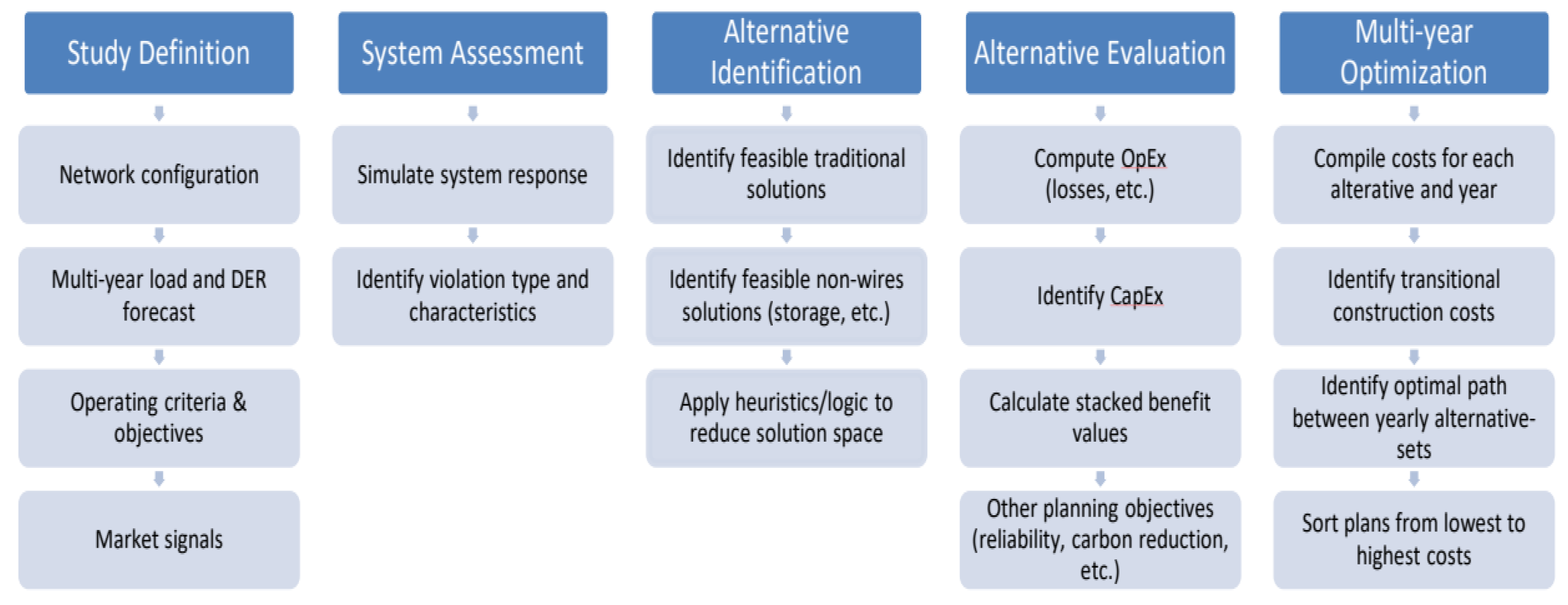
As shown in Figure 1 [2], for deciding the size and timing of the distribution facility installation in the future, the distribution line capacity should be planned in consideration of the load. Hence, it is important to forecast future loads [6]. Recently, the renewable energy connection to the distribution system is a factor that makes such forecasts more difficult. In the modern distribution plan, since it is necessary to finally establish a mid- to long-term expansion plan for distribution facilities by synthesizing the results of the forecasting renewable energy sources and loads [7], the accuracy of load forecasting for distribution lines is becoming more important than in the past, being the basis for effective and economic planning.

While the short-term load forecasting of distribution lines is necessary for operating distribution systems, the mid- to long-term load forecasting provides very important information for operation, planning, and investment [6]. In the past distribution plans, load forecasting assumed a constant increase in load; however, this assumption was insufficient in distribution plans because the mid- to long-term load forecast has a non-linear characteristic. Therefore, in addition to power data, statistical models such as the regression model and the auto-regressive integrated moving average (ARIMA) model that use population information and economic indicators as input variables were used, and currently, machine learning models such as the artificial neural network (ANN) and support vector machine (SVM) are used for load forecast [8,9]. Recently, hybrid models that combine two or more models to solve the bias problems in machine learning models and improve forecasting accuracy are being developed [10,11,12].

Currently, Korea Electric Power Corporation (KEPCO) is applying the simple linear regression method in the mid- to long-term load forecasting for the expansion plan of distribution lines, so improving accuracy is needed [13]. Therefore, it is necessary to analyze the mid- to long-term load forecasting method for the existing distribution planning. This paper derived optimal individual forecasting models based on selecting input variables for load forecasting through correlation analysis. Then, ensemble load forecasting using combining individual models was developed. In addition, this paper proposed a method for improving forecasting results by considering the characteristics of each distribution line, and the process of the mid- to long-term distribution line load peak forecasting for distribution planning was also presented. In the end, this paper verified the performance of the proposed method by comparing the forecasting with their actual values.

2. Analysis of Load Forecasting Method for the Current Distribution Planning

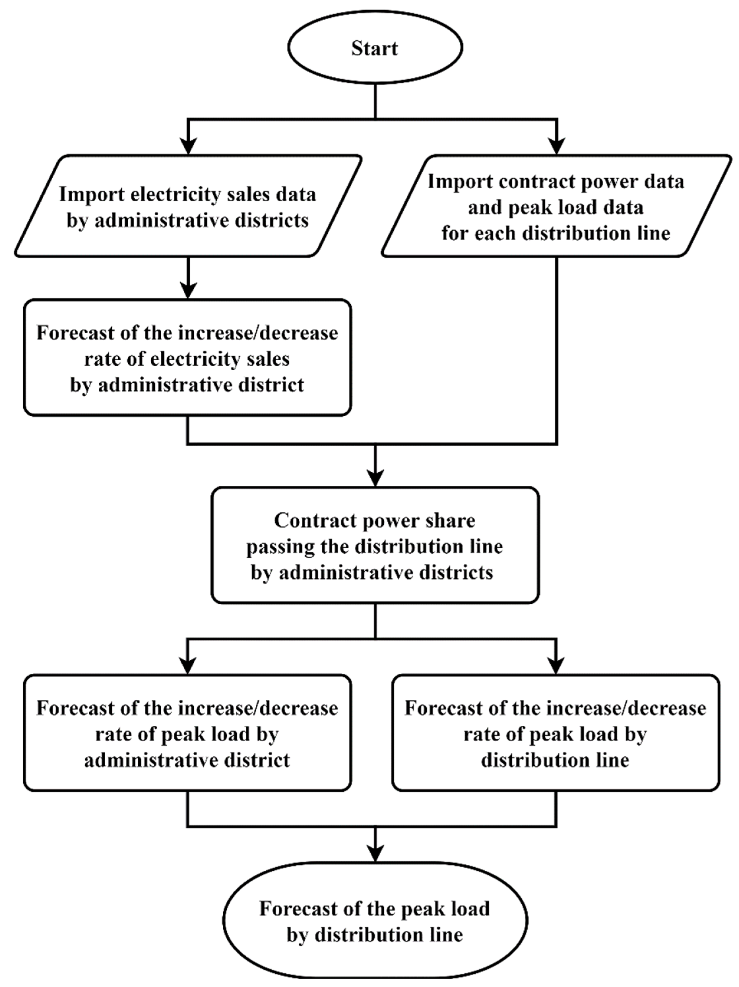
The mid- to long-term distribution line peak load forecasting process currently used by KEPCO is briefly shown in Figure 2. The algorithm forecasts the increase and decrease in the rate of electricity sales by applying the simple linear regression method to the amount of electricity sold in each administrative district. By deriving the share of contract power in each administrative district, the amount of electricity that the distribution line is responsible for by the district is calculated. Then, the increase and decrease rate of the peak load for each administrative district and each distribution line are forecasted, and then the peak loads of distribution lines are forecasted by applying these rates to each distribution line. The reason for calculating the peak loads of distribution lines is to reinforce power facilities to maintain the safety and reliability of the distribution system in mid- to long-term [13].

However, problems related to forecasting and synthesizing the peak load for each distribution line can occur. In general, the load does not increase evenly for each distribution line, and the increase and decrease rate of the load is not simple to express as a simple linear function. If distribution line peak loads are forecasted by simply applying the increase and decrease rates of the load, there is a possibility that a large error may occur. When comparing forecasting values from 2011 to 2020 according to the current distribution line peak load forecasting method as of 2010 with the real distribution line peak load values obtained from the substation operating results management system (SOMAS) within the same period, it is analyzed that the error rate increased from an average of 19% to 52% as the forecasting year approached 2020.

It can be observed from these results that the present load forecasting algorithm based on the simple linear regression method has a limitation in the optimal distribution planning. The linear regression method has the advantage of high robustness when the prediction period is long and when data are small; however, it may reach a limit in forecasting accuracy as non-linear characteristics occur in mid- to long-term forecasting because of various external variables such as weather and economy affecting the load in the distribution system. Therefore, if a machine learning technique that can improve accuracy while reflecting the influence of various external variables is applied, improved accuracy can be expected for the mid- to long-term peak load forecasting for distribution lines.

3. Selection of Input Variables for Peak Load Forecasting of Distribution Lines

Machine learning derives output values as close to real ones as possible by learning weights and biases between input variables, hidden layers, and output values and selects output values depending on the range of input variable values like a decision tree [14]. In the mid- to long-term distribution line peak load forecasting model, social, economic, and meteorological variables are used as input variables, and output values are the peak load data of each distribution line. The input variables and peak load data must be synchronized with the forecasting time series unit desired by users through preprocessing. For the mid- to long-term distribution planning, the annual peak load of distribution lines must be presented as the results of the load forecasting method. However, since annual data are insufficient to train a machine learning model, the load forecasting algorithm is configured by a monthly peak load forecasting model with monthly data. Additionally, the annual peak load forecasting value is derived from the results of the monthly forecasting model.

3.1. Definition of Data for Forecasting

Table 1. List of load data.

Description		Area
Data	Hourly	By regional headquarters nationwide (Seoul, Gyeonggi, Incheon, Gangwon, Chungbuk, Daejeon-Sejong-Chungnam, Daegu, Jeonbuk, Gwangju-Jeonnam, Gyeongnam, Busan-Ulsan, Jeju)
	Monthly
	Daily

shows the list of load data for KEPCO’s distribution lines. The data has been measured and obtained from KEPCO’s supervisory control and data acquisition (SCADA) system, used to train the distribution line peak load forecasting model. Namely, these peak load data were used as the output values lines in the mid- to long-term distribution line peak load forecasting model using machine learning. The time series units of the peak load data were provided by the hour, day, and month, and hourly data represents the most detailed load profile. The hourly data were applied to the forecasting model through the preconditioning process.

External variables such as social, economic, and meteorological variables should be used for mid- to long-term load forecasts. Data on social and economic variables were obtained from the Korean statistical information service [15], and meteorological information was obtained from the Korean weather information website [16]. The conditions for collecting social and economic variables must be time-series data for time series learning of the machine learning model and should be updated so that the constructed model can be continuously used. In other words, as much data as possible are required to forecast the load after the current point in time, and it is necessary to collect new data every year to continuously use the forecasting model in the future. A total of 597 input variables satisfying these conditions were collected, as shown in

Table 2. List of input variables for load forecasting.

Name of Data	Number of Input Variables
GDP-related variables	52
GDP deflator, real GDP, nominal GDP	3
GRDP by each economic activity	84
GRDP per capita	4
SMP, Unit price for settlement	2
Index of All industry production (original index)	5
Index of All industry production (seasonally adjusted index)	5
Population (by age, sex)	72
Composite indexes of business indicators	22
Index of equipment investment	40
Consumer price index according to purpose	13
Consumer price index by each item’s characteristic	26
Producer Price Index	260
Weather	9
Total	597

below.

3.2. Preprocessing of Input Variable Data

Social, economic, and meteorological variables have different units of time series depending on the data provided. The process of preconditioning them into monthly data is required to use them as input values for the machine learning model. Data provided in a detailed cycle, such as weather, can be collected by selecting monthly data. However, gross domestic product (GDP), gross regional domestic product (GRDP), and population are economic and social indicators calculated and provided by year. Therefore, in order to use annual data as input variables for load forecasting, it should be estimated as monthly data based on the interpolation method. As shown Figure 3, nominal GRDP’s monthly data were estimated by the cubic curve fitting interpolation method.

3.3. Input Variable Selection Process

Forecasting performance depends on the combination of input variables in machine learning and deep learning-based forecasting [10]. It is necessary to construct a forecasting model by collecting and analyzing multiple input variables. Final input variables for distribution line peak load forecasting should be selected, and a forecasting model should be presented by comparing the performance of forecasting models according to the combination of input variables through correlation analysis of input variables and output variables such as Pearson correlation, Spearman correlation, and mutual information analysis [17,18,19,20,21,22]. Figure 4 shows the input variable selection process for constructing a machine learning model.

3.3.1. Deriving Forecasting Input Variables

The machine learning model has learned the relational equation between input and output values. However, the past data of input variables are insufficient to forecast accurate loads. Therefore, forecasting models need the predicted input variables for mid- to long-term peak loads forecasting. Additionally, it is necessary to verify the predictability of input variables and the performance of load forecasting with them. The long short-term memory (LSTM) model, a representative algorithm of time series machine learning, was used to forecast input variables. A simple time series model without other external input variables was applied for the input variable forecast. In addition, the period provided for each data is different; thus, the learning period was configured and forecasted using the maximum time-series data provided individually. The normalized Root Mean Squared Error ($nRMSE$) was used as an index that judges predictability. $nRMSE$ compares the degree of error between variables with different units and scales [23], as expressed in Equation (1). As shown in Figure 5a, the non-linear, noncyclic data in the agricultural index is difficult to forecast. Therefore, its $nRMSE$ is greater than 10%. Figure 5b has a trend with a linear increase, showing that its forecast results are within 10% even after training the LSTM model several times. Through this process, 23 out of 597 data inputs were selected, and the list of selected data are shown in

Table 3. List of predictable input variables.

Name of Data	Number of Input Variables
GDP-related variables	1
GDP deflator, real GDP, nominal GDP	1
GRDP by each economic activity	10
GRDP per capita	1
Population (by age, sex)	2
Consumer price index by each item’s characteristic	6
Weather	2
Total	23

. As shown in Table 3, 23 input variables were selected, including 19 economic indicators, 2 social indicators, and 2 meteorological factors such as monthly maximum and average maximum temperature.

$$nRMSE=\frac{1}{\max \left(y\right)-\min \left(y\right)}\sqrt{{\displaystyle \sum }_{i=1}^n\left(\frac{{\left(\widehat{y_i}-y_i\right)}^2}{n}\right)}\times 100$$

(1)

3.3.2. Input and Output Correlation Analysis

After deriving forecasting input variables, variables that would increase the interpretability of machine learning are selected through input and output correlation analysis. The relationship between the characteristics of the overall peak load and input variables in the target area is identified through a correlation analysis. The correlation was analyzed using the Pearson correlation coefficient, Spearman correlation coefficient, and the mutual information index. The mutual information is called interdependence information and is an indicator that can determine the correlation between two data sets in addition to the linear correlation. The Pearson correlation coefficient, which is often used in correlation analysis, analyzes linear correlations, and the Spearman correlation coefficient has a high correlation even in the case of non-linear monotonic functions by analyzing the linear correlation of rank [17,18,19,20,21,22].

Figure 6 and Figure 7 show the results of analyzing the correlation coefficients of 46 input variables, representing that the first row or column shows the correlation between the month peak and other input variables. Variables in dark blue have high correlation coefficients. In general, a correlation coefficient of 0.7 or more indicates that the linear correlation coefficient is high, and thus variables with a Pearson correlation coefficient or a Spearman correlation coefficient of 0.7 or higher were selected [24]. When neither correlation coefficient satisfied the criterion of 0.7, mutual information was performed. Although the correlation coefficients of the monthly maximum and average maximum temperature were not satisfied with 0.7, it was analyzed that the periodic correlation was high as shown in Figure 8 through mutual information. Accordingly, 23 input variables were finally selected.

4. Mid- to Long-Term Distribution Line Peak Load Forecasting Model

4.1. Implementation of the Machine Learning Model and Selection of Optimal Learning Period

The configuration of the hidden layer depends on the machine learning algorithm, and layer configuration and the number of nodes can be selected by user settings. In particular, the decision tree-based model has slightly different performance and characteristics depending on the ensemble method applied in the tree. Although each forecast model has its own characteristics, its performance depends on the forecasting cycle and data composition. Hence, it is necessary to analyze various models before selecting one [25,26,27].

First, as for artificial neural network-based time series machine learning models, there are many types of artificial neural network (ANN)-based models, such as recurrent neural network (RNN), deep neural network (DNN), and convolutional neural network (CNN), depending on the layer configuration [25,28]. Among them, the LSTM and gated recurrent unit (GRU) models are representative RNN-based models that are advantageous for time series learning by receiving a sequence as an input. In addition, there are different types of decision tree-based machine learning models depending on the ensemble method. Bagging and boosting are typically used in decision tree ensembles. Random Forest is a representative bagging ensemble model, and LSBoost is a typical boosting ensemble model [26]. These models were selected as forecasting algorithms for mid- to long-term load forecasting.

It is necessary to derive the optimal learning period by comparing the performance of the LSTM, GRU, Random Forest, and LSBoost models. Load data of distribution lines belonging to KEPCO’s Gimje substation were obtained from SOMAS for 18 years (from 2003 to 2020). As shown in Figure 9, tests were conducted with different learning periods to guarantee sufficient learning data with fixed the same forecasting verification period. The forecasting verification period was fixed at eight years, and the learning periods varied from three to ten years, as in Figure 9, with the results shown in

Table 4. Performance results by learning period.

Index	Test 1	Test 2	Test 3	Test 4	Test 5	Test 6	Test 7	Test 8	Avg.
MAE	1.27	1.25	1.24	1.29	1.30	1.38	1.64	1.37	1.34
MSE	2.83	2.99	2.64	2.94	2.80	3.27	4.99	3.15	3.20

. The mean absolute error (MAE) and mean squared error (MSE), expressed in Equations (2) and (3), were used to assess forecast results obtained by machine learning models. They measure the difference between the original and predicted values. As shown in Table 4, the predicted performance of the four machine learning forecasting models was better than the others when the training period was over eight years. Therefore, at least an eight-year learning period is required for good performance load forecasting of eight years.

$$\mathrm{MAE}=\frac{1}{n}{\displaystyle \sum }_{i=1}^n\left|\widehat{y_i}-y_i\right|$$

(2)

$$\mathrm{MSE}=\frac{1}{n}{\displaystyle \sum }_{i=1}^n{\left(\widehat{y_i}-y_i\right)}^2$$

(3)

4.2. Optimal Ensemble Model Combination

The ensemble model is proposed to compensate for individual models’ shortcomings and improve the forecasting performance. Ensemble models include bagging, boosting, voting, and stacking methods. The bagging and boosting methods aforementioned separate data from the same model and combine multiple training results, respectively. While the voting method selects forecast results of a model that shows high performance during verification among different forecasting models, the stacking method uses predicted results of different forecasting models as input variables and the actual values as output variables to construct the learning model again [27]. The bagging and boosting ensemble methods are not suitable for combining different models, and it is difficult to see the voting method as a combination of models because it simply selects the forecasting results of one model. Accordingly, the stacking method is appropriate for improving forecast accuracy based on different machine learning models.

Four previously selected forecasting models, LSTM, GRU, random forest, and LSBoost, are combined into a stacking ensemble model through DNN. Compared with the ANN, the DNN model has higher performance as the complexity increases because the number of hidden layers and nodes increases and can derive non-linear predictive values that cannot accurately identify the relationship, unlike the regression model. DNN models are generally used more than simple machine learning or ANN models in recent studies with increased computing power [25]. Depending on the detailed DNN structure, there are various derivative models such as CNN and RNN. While CNN is a modified structure to analyze patterns such as images, the RNN can predict sequential and repeating inputs [25,28]. However, since the stacking ensemble is a structure for deriving more accurate values for the output values of individual models, a simple DNN model can be used in the stacking ensemble.

In the case of selecting two years of an ensemble study period,

Table 5. Comparison of forecasting performance of ensemble models.

Combination of Forecasting Models	Number of Forecasting Models	MAE	MSE
Random Forest + LSTM + GRU + LSBoost	4	0.9465	1.9849
Random Forest + LSTM + GRU	3	0.8863	1.4224
Random Forest + LSTM + LSBoost	3	0.9723	2.1536
Random Forest + GRU + LSBoost	3	0.9663	0.9838
LSTM + GRU + LSBoost	3	1.0378	2.2369
Random Forest + LSTM	2	0.9182	1.5057
Random Forest + GRU	2	0.8942	1.4793
Random Forest + LSBoost	2	1.0116	2.4720
LSTM + GRU	2	1.1673	2.0823
LSTM + LSBoost	2	1.1351	2.5318
GRU + LSBoost	2	1.1183	2.5217

compares the performance of 11 ensemble models over the 8-year verification period by various combinations of four machine learning models. In particular, three models, random forest + LSTM + GRU, random forest + LSTM, and random forest + GRU showed higher performance than other models. As a result, random forest + LSTM + GRU was selected as the most representative ensemble model considering the performance index.

The disadvantage of the stacking ensemble method is that the output values of multiple different forecasting models need to be trained; hence its learning period is relatively longer. The selected random forest + LSTM + GRU ensemble model is applied for one and two years, and the resultant forecasting performance is listed in

Table 6. Comparison of forecasting performance by ensemble learning period. Tests 1 and 2 represent one- and two-year tests, respectively.

	MAE	MSE	Error Rate (%)
Test 1	2.2548	8.7153	41.1126
Test 2	0.8863	1.4224	12.4454

. Each model was learned for eight years, and the learning period of the ensemble model was different. Each ensemble model was forecasted for eight years from 2013 to 2020. It is necessary to distinguish individual learning models and ensemble learning models among the given data because of the nature of the stacking ensemble. The learning period of the individual time series machine learning model that applies recent trends is reduced to increase that of ensemble learning. Therefore, it is necessary to construct an efficient ensemble model with a shorter period. According to Table 6, the case of learning for one year shows very poor performance compared with the case of ensemble learning for two years. The shorter the ensemble learning period, the longer the learning period can be invested in the time series learning model. Finally, the two-year is proper will proper for the ensemble model based on the acquisition data period.

It compared the performance of applying the ensemble model with that of individual learning models by setting their verification period for eight years (from 2013 to 2018). As shown in

Table 7. Comparison of ensemble and individual model prediction performance.

Forecasting Model	MAE	MSE	Error Rate (%)
Ensemble	0.8863	1.4224	12.4454
Random Forest	1.3324	2.8062	16.4040
LSTM	1.1785	2.6965	16.1125
GRU	1.1376	2.3738	15.2158
LSBoost	1.3909	3.3398	21.0127

, the ensemble model has the best predictive performance compared to the individual models.

The proposed Random Forest + LSTM + GRU ensemble model structure is shown in Figure 10. In addition,

Table 8. Forecast verification error percentage of the Gimje substation distribution lines.

Substation	Number of D/Ls	2013	2014	2015	2016	2017	2018	2019	2020	Avg.
Gimje	15	7.54	10.99	16.39	19.44	11.21	9.49	9.72	14.79	12.45

shows the peak load forecasting error percentage of the actual 15 distribution lines connected to the Gimje substation of the KEPCO Gimje Branch Office, which was verified with the ensemble model finally proposed.

5. Development of Peak Load Forecasting Process Considering Distribution Line Characteristics

As in Table 8, the proposed mid- to long-term distribution line peak load ensemble forecasting model has improved forecasting accuracy compared to the previous linear regression-based peak load forecasting method. However, a distribution line may not meet the learning period of the forecasting model because many new distribution lines are newly built every year or may change owing to load switching. This learning period problem may impair forecasting accuracy, so a peak load forecasting process that reflects the characteristics of such distribution lines is required.

5.1. Forecasting Model Reflecting Load Fluctuations of Distribution Lines

In the distribution system, a new distribution line may cause load transfer and movement, thus changing distribution line loads. As a result, the peak load pattern of the distribution line may also change significantly. In such a case, even if the proposed ensemble model is applied, the forecasting accuracy may be impaired because external input variables do not cause the change.

For solving this problem, an outlier detection algorithm is applied in a statistical manner. The annual maximum load change rate for each power distribution line was derived, and the outlier of the change rate was derived. Then, outliers can be detected by Equation (4), which is based on the outliers scaled by multiplying the constant by the MAD as used in the statistical outlier calculation method [29].

$$\mathrm{MAD}=\mathrm{c}\times \mathrm{median}\left(\left|X_i-\mathrm{median}\left(X\right)\right|\right), c=-\frac{1}{\sqrt{2}\times \mathrm{erfcinv}\left(\frac{3}{2}\right)}=1.4826$$

(4)

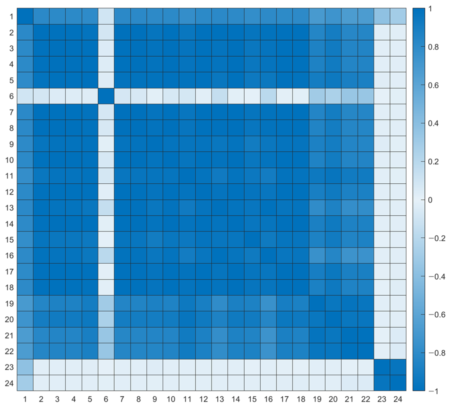
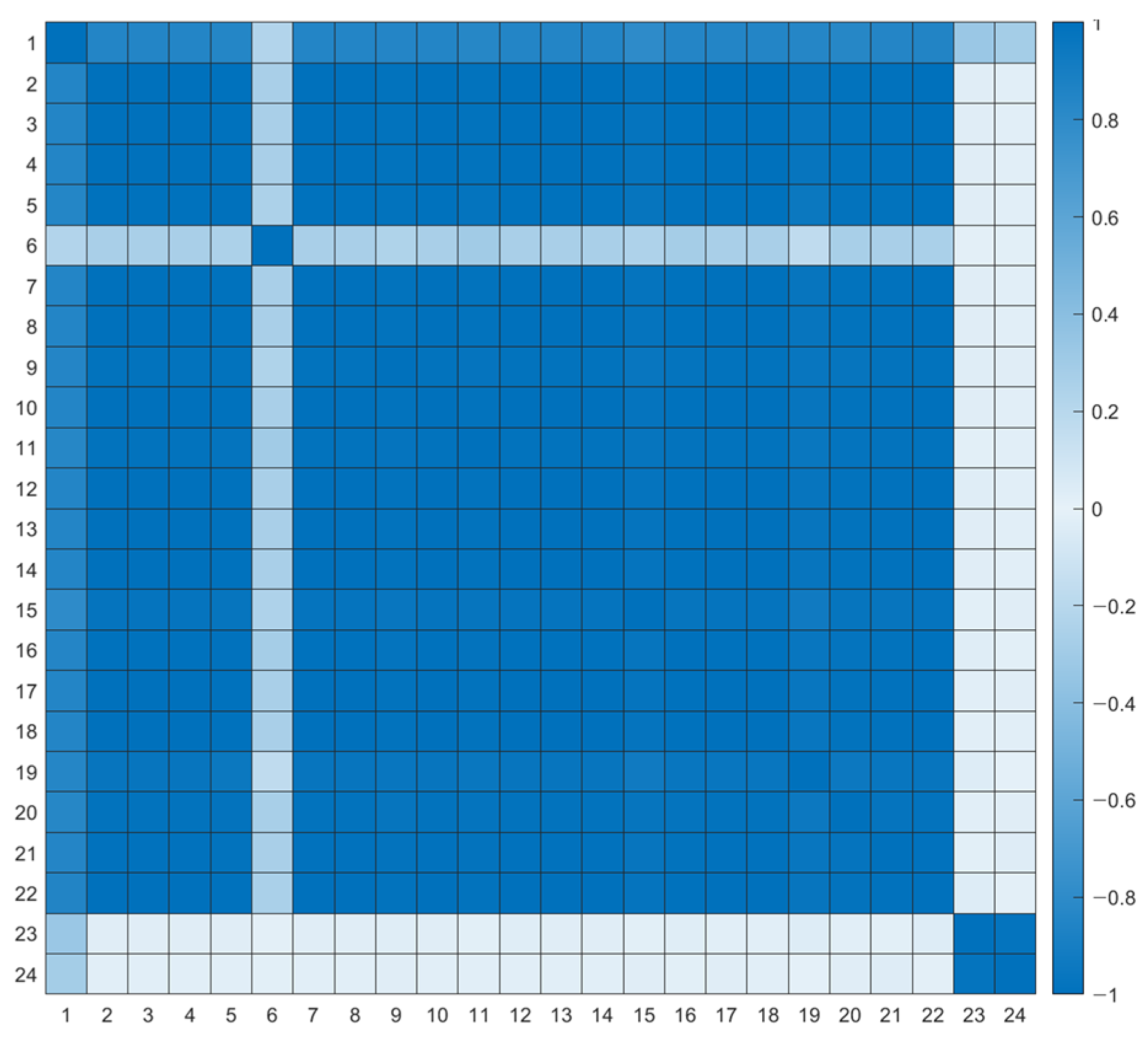
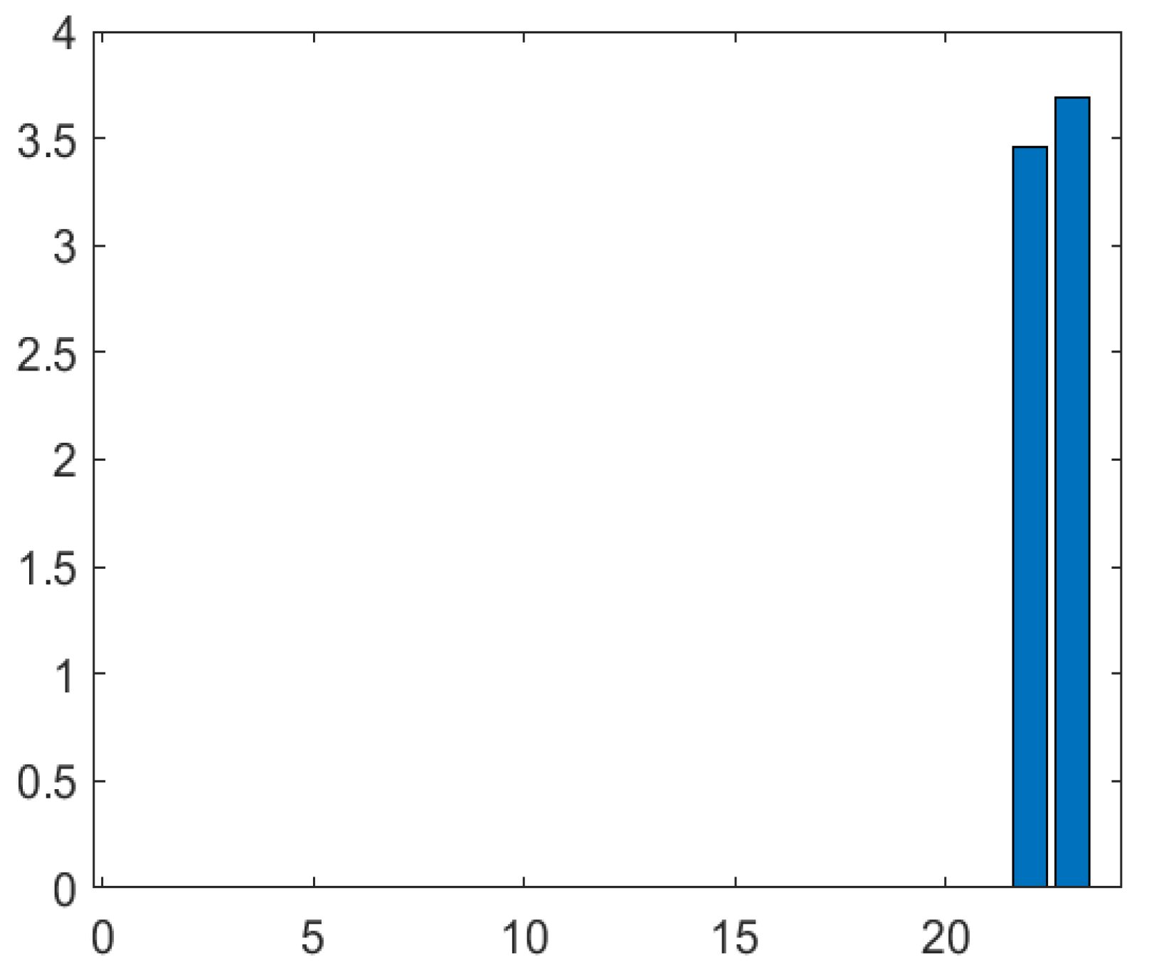
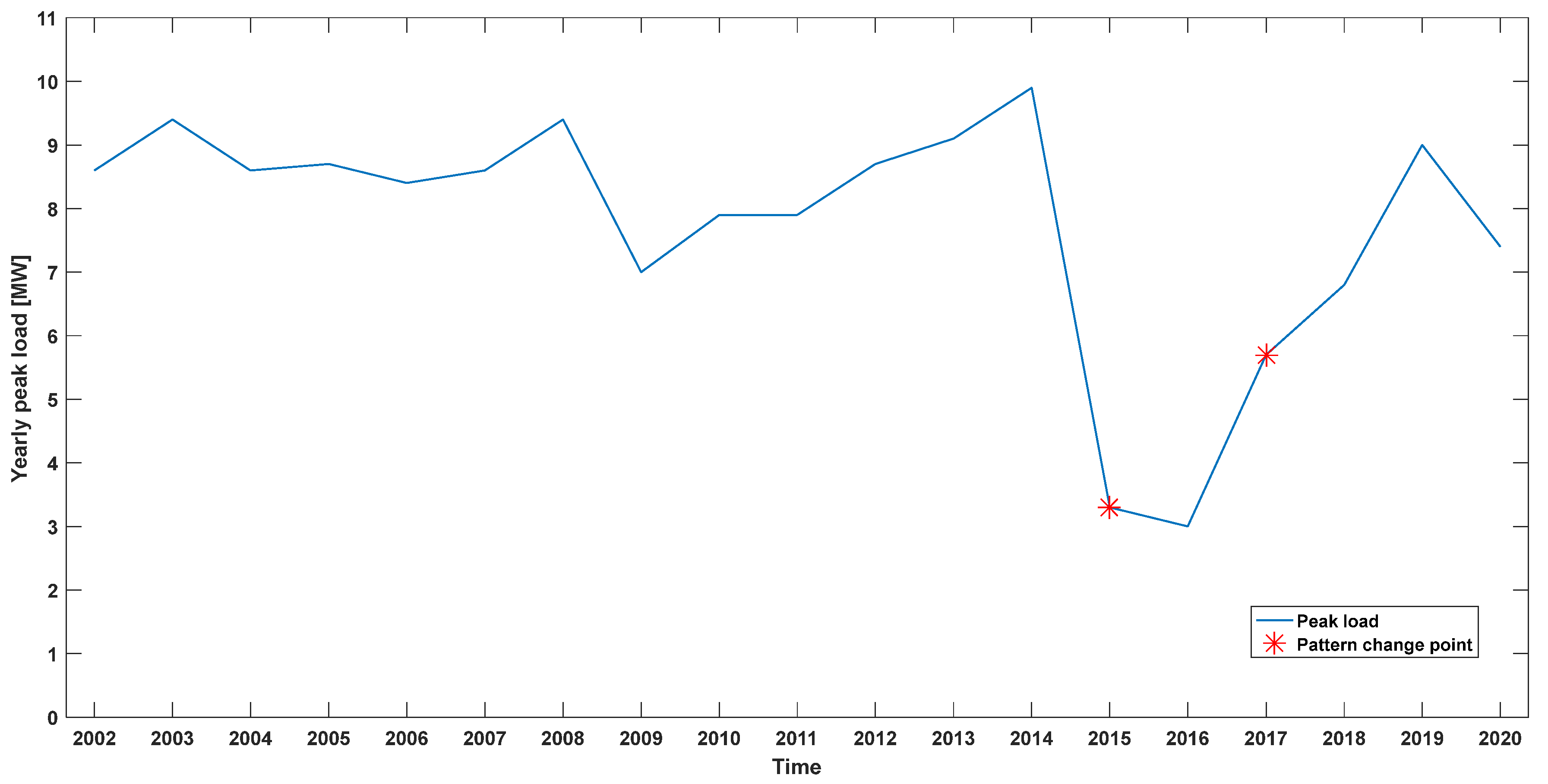
Since the pattern characteristics are different for each distribution line, outlier criteria were selected by the rate of yearly peak change for each distribution line. The rate of change in the monthly peak average was defined as the rate of change in the interval based on the period when the annual peak rate of change was large. As shown in Figure 11, the pattern change was applied by displaying the pattern and calculating the average value ratio between the pattern change intervals.

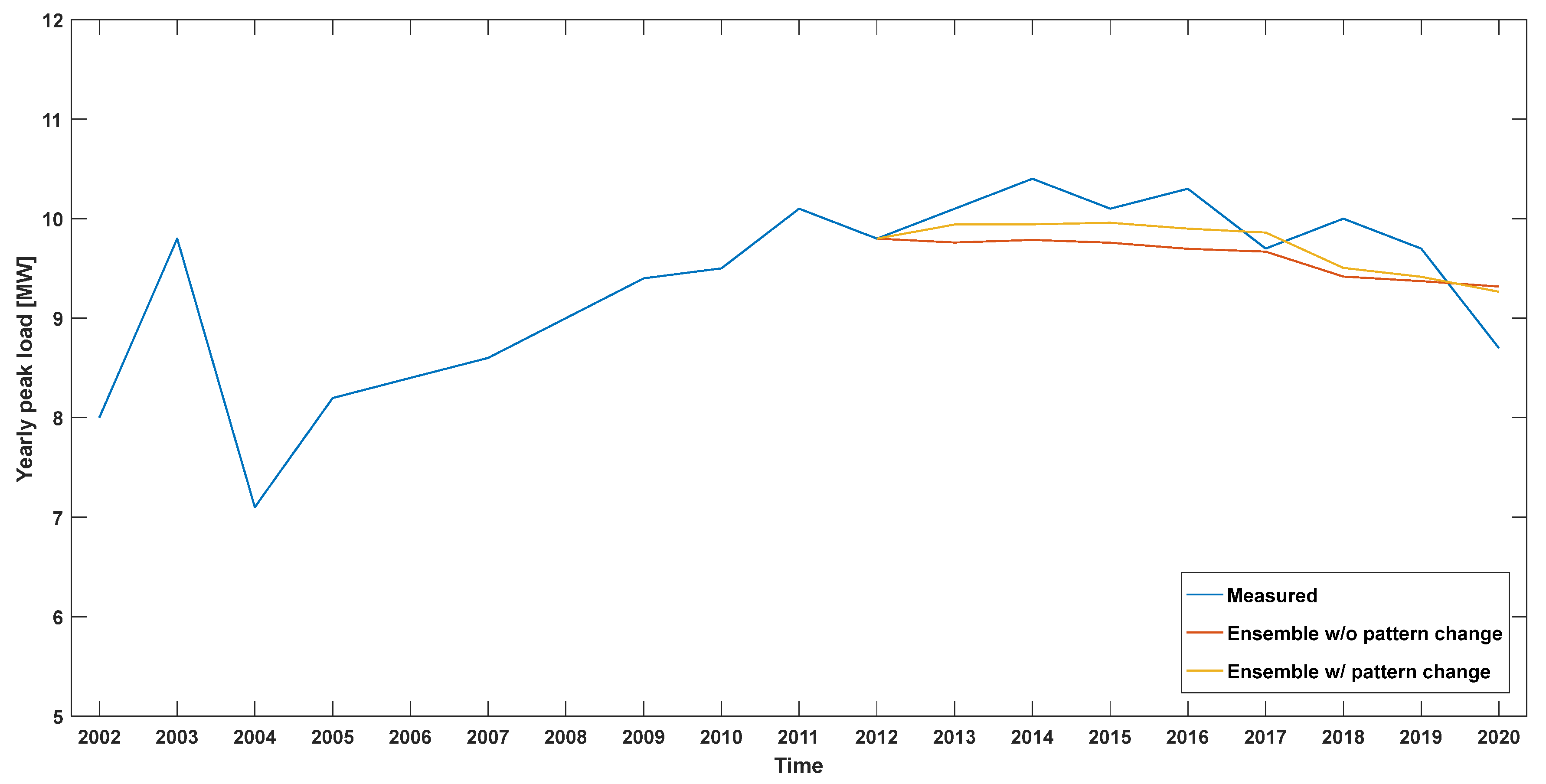
This pattern change point and interval average change were applied to the ensemble forecasting model. As shown in Figure 12, pattern changes occur within the learning period. In this case, the entire learning data are integrated into the latest pattern to follow it. This approach does not learn irrelevant patterns and provides sufficient learning data for one pattern. As shown in Figure 12, when one of the distribution lines belonged to the Gimje substation, the overall peak load change was minor, but large pattern changes were found in 2004 and 2005. Figure 12 shows the result of comparing the forecasting model with and without applying the pattern change algorithm to the distribution line. By correcting 15 distribution lines at the Gimje substation with the pattern change algorithm, it was confirmed that the forecasting performance improved, as shown in

Table 9. Performance results with and without applying the pattern change algorithm.

Pattern Change Algorithm	MAE	MSE	Error Rate (%)
Before → Not applied	0.8863	1.4224	12.4454
After → Applied	0.8329	1.2229	11.4882

.

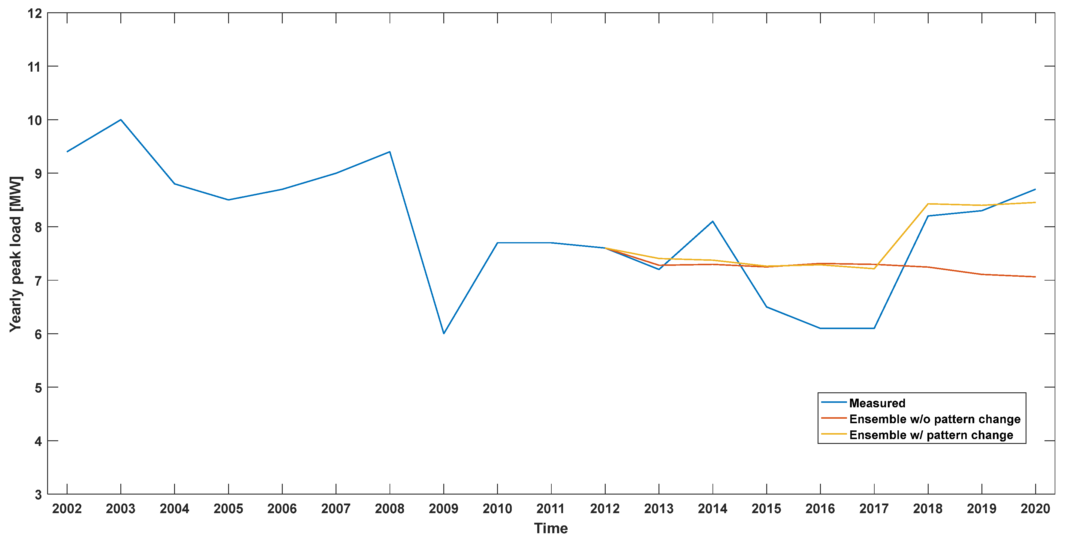
Another noticeable case is when a pattern change occurs during the forecast period. In this case, the timing and rate of change of the load pattern are known since the load transfer and movement of distribution lines are planned. There is no pattern change during the learning period, thus learning the data as they are. Instead, a pattern change with an average change rate during the forecast period is applied to forecast output values. It can be seen from Figure 13 that a pattern change occurs during the forecast period of one of the distribution lines at the Gimje substation. When applying the pattern change approach proposed, the same verification period for eight years, from 2013 to 2020, was analyzed for the ensemble model.

Table 10. Performance results with and without applying the pattern change algorithm for the forecast period.

Pattern Change Algorithm	MAE	MSE	Error Rate (%)
Before → Not applied	0.8863	1.4224	12.4454
After → Applied	0.8719	1.2817	10.9126

shows that the forecast results improve as compared with the case where pattern change was not applied. In the end, it was verified that the pattern change algorithm could further improve the forecast accuracy in the case of load transfer or movement, which is the characteristic of the distribution line.

5.2. Forecasting Model of Distribution Lines with Insufficient Learning Period

The proposed peak load forecasting requires ten years of the training period, comprising eight years of individual model training and two years of ensemble model training. However, since many new distribution lines are installed every year, some distribution lines inevitably lack the learning period. Therefore, the distribution line with an insufficient learning period should be separated in the load forecasting process, and a separate load forecasting model should be applied to the distribution line. A machine learning model with better performance than the previous regression method needs to be used when the learning period is short.

The 170 distribution lines of KEPCO’s Gunsan branch office were considered for the case study.

Table 11. Number of distribution lines that can be forecasted by the proposed peak load forecasting method according to the learning period in Gunsan branch office.

Test	Number of D/Ls
1	129
2	121
3	116
4	109
5	104
6	98
7	97
8	96
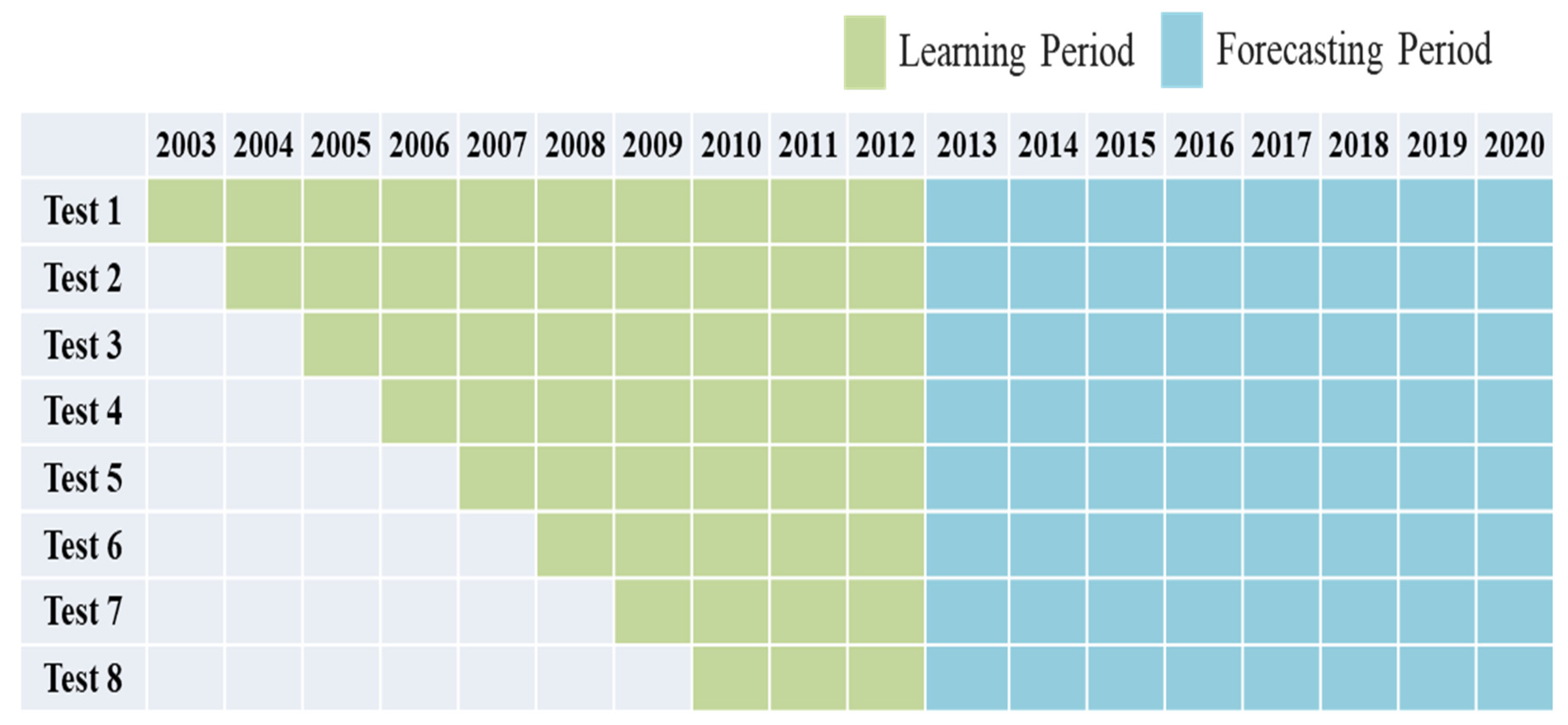
9	94
10	57

lists the number of distribution lines that can be forecasted according to the different learning periods; to be specific, the test number is identical to the years assigned for the learning period. Table 11 indicates that the number of distribution lines that could be forecasted decreased with the learning period since there was a limited period of total data collected.

Table 12. Performance comparison among single forecasting models for the different learning period.

Forecasting Model	Index	Test 1	Test 2	Test 3	Test 4	Test 5	Test 6	Test 7	Test 8	Test 9	Test 10	Avg.
GRU	MAE	1.77	2.02	1.71	1.79	1.61	1.68	1.62	1.57	1.48	1.28	1.65
	MSE	2.36	2.24	2.60	2.75	2.39	3.18	6.33	3.17	4.34	3.18	5.07
LSTM	MAE	1.85	1.68	1.17	1.62	1.56	1.60	1.52	1.43	1.46	1.31	1.52
	MSE	6.28	5.32	5.20	4.73	4.48	4.70	4.52	4.09	4.28	3.20	4.68
Random Forest	MAE	1.81	1.61	1.56	1.53	1.52	1.51	1.48	1.49	1.49	1.31	1.53
	MSE	5.27	4.28	4.26	4.16	4.18	4.14	4.05	4.05	4.07	3.28	4.17
LSBoost	MAE	1.30	1.47	1.35	1.41	1.42	1.40	1.41	1.48	1.31	1.33	1.39
	MSE	3.43	3.87	3.69	3.95	3.64	3.74	3.82	3.77	3.46	3.27	3.66

lists the performance test results of single machine learning models for different learning periods. The verification period was eight years, from 2013 to 2020. Since the learning period was insufficient, tests with various learning periods were required. As shown in Table 12, the LSBoost model with the best performance results was selected as the load forecasting model for distribution lines with a short learning period.

Table 13. Comparison of error percentage with the existing regression method and the LSBoost model.

Forecasting Model	2013	2014	2015	2016	2017	2018	2019	2020	Avg.
Regression	27.26	28.37	30.61	39.14	36.21	41.59	48.46	51.98	37.95
LSBoost	12.68	16.85	17.58	17.49	18.35	17.28	19.71	17.48	17.18

shows the performance comparison between the existing regression forecasting model and the proposed LSBoost forecasting model for the 170 distribution lines of KEPCO’s Gunsan branch office, where learning data exists for more than one year. Table 13 indicates that the average error of 32% was significantly improved to 17% when the LSBoost model was used. All in all, with the distribution line that lacks the training period, the single LSBoost model has superior forecasting performance compared with the conventional regression method.

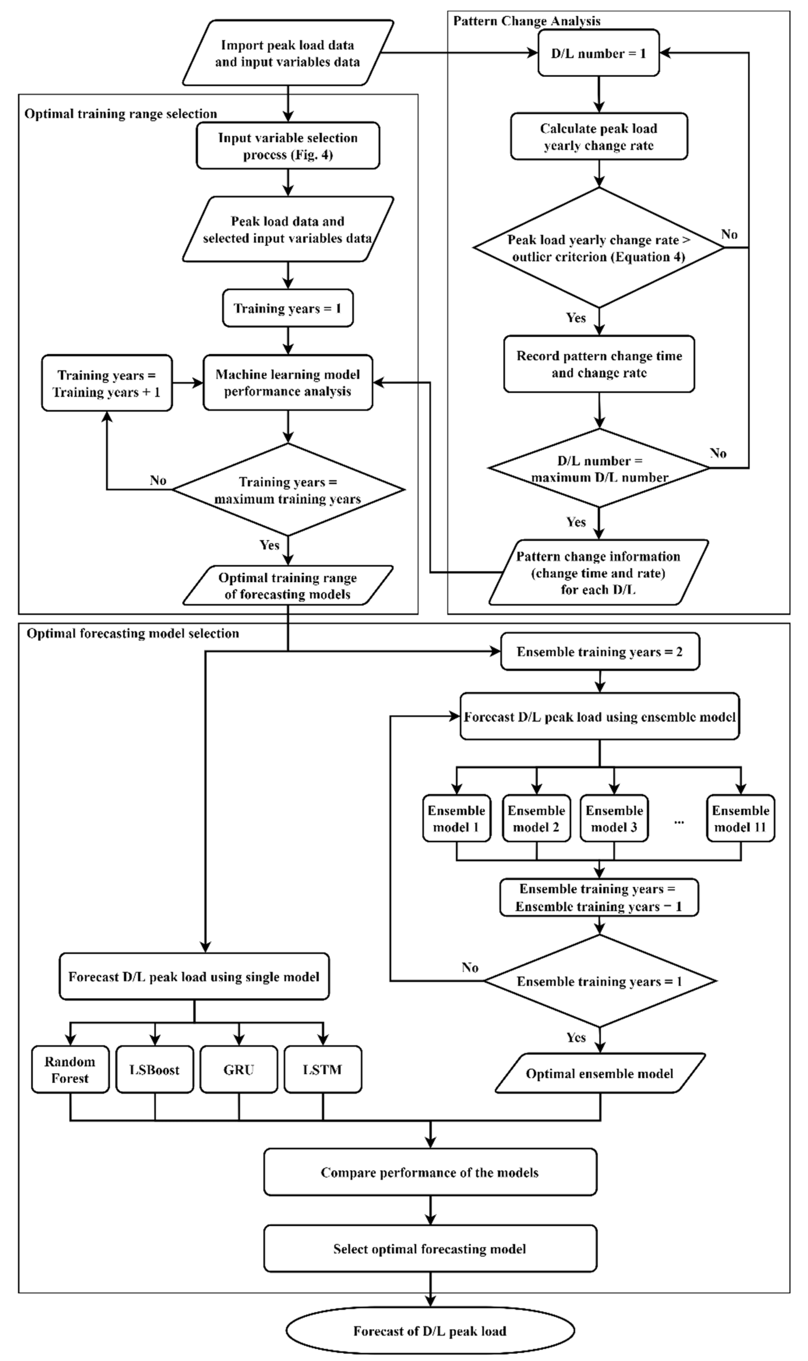
5.3. Distribution Line Peak Load Forecasting Process for Mid- to Long-Term Distribution Planning

Figure 14 shows the proposed mid- to long-term distribution line peak load forecasting process for distribution planning based on the ensemble model. This process improved the forecasting accuracy for the load fluctuation and lack of learning period of the distribution line while providing improved predictions compared to the conventional load forecasting method for all distribution lines.

Table 14. Forecasting error percentage of all distribution lines at the Gimje substation.

Substation	Number of D/Ls	2013	2014	2015	2016	2017	2018	2019	2020	Avg.
Gimje	22	9.91	13.88	14.41	13.24	12.97	12.80	14.90	17.35	13.68

shows the forecasting verification results for all 22 distribution lines connected to the KEPCO Gimje substation using the proposed load peak forecasting process. The 22 distribution lines of the Gimje substation had severe load fluctuations and insufficient learning periods. As shown in Table 14, the 8-year accuracy of the distribution line peak load forecasting was 87% on average.

Table 15. Comparison of forecast performance between the existing and proposed model at the Gimje substation.

	MAE	MSE	Error Rate (%)
Existing regression model	2.0518	7.6819	27.7015
Proposed forecasting model	1.2227	2.7609	13.6837

compares forecast performance between the existing regression forecasting and the proposed model, indicating that the MAE, MSE, and error rate were significantly improved. It was verified that the proposed peak load forecasting process for mid- to long-term presented higher forecast accuracy than the existing method. The efficiency of investment can be improved by the accuracy of the timing and capacity in distribution planning with the proposed forecasting process.

6. Conclusions

As the environment of the distribution system changes rapidly due to the expansion of renewable energy, the importance of distribution planning is growing. Therefore, this paper proposed the model and process for load forecasting, which is the essential element in distribution planning. The optimal ensemble machine learning model was derived to overcome the limitations of the non-linear characteristics of the existing linear regression load forecasting method for the mid- to long-term. The optimal input variables and the learning period were selected. This paper presented the ensemble model for forecasting the peak load for the mid- to long-term distribution lines and verified the result through KEPCO’s power data. The proposed method also reflected distribution line characteristics such as load fluctuations and lack of the learning period for its application to all distribution lines of power utilities. Its performance was verified by actual data from distribution lines at the KEPCO Gimje substation. In the future, KEPCO plans to implement the distribution load forecasting system based on the proposed process of updating power data and external data. Additionally, it will be used to plan the distribution planning for the mid-to long-term. In particular, it will help to make investment decisions for distribution substations and feeders. It will be expected that efficient and economical distribution planning will be enabled even in a distribution system situation where uncertainty increases.

References

1. Willis, H.L. Power Distribution Planning Reference Book, 2nd ed.; Marcel Dekker: New York, NY, USA, 2004. [Google Scholar]
2. Roark, J.D.; O’Connell, A.; Taylor, J. An Advanced Distribution Planning And Optimization Process. In Proceedings of the 25th International Conference on Electricity Distribution (CIRED), Madrid, Spain, 3–6 June 2019; p. 2131. [Google Scholar]
3. Chae, W.; Lee, H.; Park, J.; Jung, W. Cooperative operation method of two battery systems at Microgrid system. In Proceedings of the 3rd IEEE International Symposium on Power Electronics for Distributed Generation Systems (PEDG), Aalborg, Denmark, 25–28 June 2012; pp. 872–877. [Google Scholar]
4. Kim, J.; Kim, H.; Cho, J.; Cho, Y.; Cho, Y.; Kim, S. Demonstration Study of Voltage Control of DC Grid Using Energy Management System Based DC Applications. Energies 2020, 13, 4551. [Google Scholar] [CrossRef]
5. Smith, J. Distribution Planning Guidebook for the Modern Grid: Installment 2; EPRI: Palo Alto, CA, USA, 2016. [Google Scholar]
6. Chemetova, S.; Santos, P.J.; Ventim-Neves, M. Load peak forecasting in different load patterns situations. In Proceedings of the 10th International Conference on Compatibility, Power Electronics and Power Engineering (CPE-POWERENG), Bydgoszcz, Poland, 29 June–1 July 2016; pp. 148–151. [Google Scholar]
7. Olearczyk, M. Load Forecasting for Modern Distribution Systems; EPRI: Palo Alto, CA, USA, 2013. [Google Scholar]
8. Torkzadeh, R.; Mirzaei, A.; Mirjalili, M.M.; Anaraki, A.S.; Sehhati, M.R.; Behdad, F. Medium term load forecasting in distribution systems based on multi linear regression & principal component analysis: A novel approach. In Proceedings of the 19th Conference on Electrical Power Distribution Networks (EPDC), Tehran, Iran, 6–7 May 2014; pp. 66–70. [Google Scholar]
9. Waseem, M.; Lin, Z.; Yang, L. Data-Driven Load Forecasting of Air Conditioners for Demand Response Using Levenberg–Marquardt Algorithm-Based ANN. Energies 2019, 3, 36. [Google Scholar] [CrossRef] [Green Version]
10. Tan, M.; Yuan, S.; Li, S.; Su, Y.; Li, H.; He, F. Ultra-Short-Term Industrial Power Demand Forecasting Using LSTM Based Hybrid Ensemble Learning. IEEE Trans. Power Syst. 2020, 35, 2937–2948. [Google Scholar] [CrossRef]
11. Pan, F.; Zhang, H.; Xia, M. A Hybrid Time-Series Forecasting Model Using Extreme Learning Machines. In Proceedings of the 2009 Second International Conference on Intelligent Computation Technology and Automation, Changsha, China, 10–11 October 2009; pp. 933–936. [Google Scholar]
12. Buluş, K.; Zor, K. A hybrid deep learning algorithm for short-term electric load forecasting. In Proceedings of the 2021 29th Signal Processing and Communications Applications Conference (SIU), Hefei, China, 25–27 February 2021; pp. 1–4. [Google Scholar]
13. Park, U. The Procedure of Forecasting Distribution Line Peak; KEPCO: Seoul, Korea, 2013. [Google Scholar]
14. Yiling, H.; Shaofeng, H. A Short-Term Load Forecasting Model Based on Improved Random Forest Algorithm. In Proceedings of the 2020 7th International Forum on Electrical Engineering and Automation (IFEEA), Hefei, China, 25–27 September 2020; pp. 928–931. [Google Scholar]
15. KOSIS (Korean Statistical Information Serveice). Available online: https://kosis.kr/eng/ (accessed on 21 February 2022).
16. Open MET Data Portal. Available online: https://data.kma.go.kr/resources/html/en/aowdp.html (accessed on 21 February 2022).
17. Cheng, J.; Zhang, N.; Wang, Y.; Kang, C.; Zhu, W.; Luo, M.; Que, H. Evaluating the spatial correlations of multi-area load forecasting errors. In Proceedings of the 2016 International Conference on Probabilistic Methods Applied to Power Systems (PMAPS), Beijing, China, 16–20 October 2016; pp. 1–6. [Google Scholar]
18. Alzate, C.; Sinn, M. Improved Electricity Load Forecasting via Kernel Spectral Clustering of Smart Meters. In Proceedings of the 2013 IEEE 13th International Conference on Data Mining, Dallas, TX, USA, 7–10 December 2013; pp. 943–948. [Google Scholar]
19. Chen, J.; Li, T.; Zou, Y.; Wang, G.; Ye, H.; Lv, F. An Ensemble Feature Selection Method for Short-Term Electrical Load Forecasting. In Proceedings of the 2019 IEEE 3rd Conference on Energy Internet and Energy System Integration (EI2), Changsha, China, 8–10 November 2019; pp. 1429–1432. [Google Scholar]
20. Huang, N.; Hu, Z.; Cai, G.; Yang, D. Short Term Electrical Load Forecasting Using Mutual Information Based Feature Selection with Generalized Minimum-Redundancy and Maximum-Relevance Criteria. Entropy 2016, 18, 330. [Google Scholar] [CrossRef] [Green Version]
21. Waseem, M.; Lin, Z.; Liu, S.; Jinai, Z.; Rizwan, M.; Sajjad, M.I.A. Optimal BRA based electric demand prediction strategy considering instance-based learning of the forecast factors. Int. Trans. Electr. Energy Syst. 2021, 31, e12967. [Google Scholar] [CrossRef]
22. Koprinska, I.; Rana, M.; Agelidis, V.G. Correlation and instance-based feature selection for electricity load forecasting. Knowl.-Based Syst. 2015, 82, 29–40. [Google Scholar] [CrossRef]
23. Keitsch, K.A.; Bruckner, T. Input data analysis for optimized short term load forecasts. In Proceedings of the 2016 IEEE Innovative Smart Grid Technologies—Asia (ISGT-Asia), Melbourne, VIC, Australia, 28 November–1 December 2016; pp. 1–6. [Google Scholar]
24. Care, F.R.A.M.; Subagio, B.S.; Rahman, H. Porous concrete basic property criteria as rigid pavement base layer in Indonesia. MATEC Web Conf. 2018, 147, 02008. [Google Scholar]
25. Hossen, T.; Nair, A.S.; Chinnathambi, R.A.; Ranganathan, P. Residential Load Forecasting Using Deep Neural Networks (DNN). In Proceedings of the 2018 North American Power Symposium (NAPS), Fargo, ND, USA, 9–11 September 2018; pp. 1–5. [Google Scholar]
26. Karthikeyan, M.; Rengaraj, R. Short-Term Wind Speed Forecasting Using Ensemble Learning. In Proceedings of the 2021 7th International Conference on Electrical Energy Systems (ICEES), Chennai, India, 11–13 February 2021; pp. 502–506. [Google Scholar]
27. Singh, S.; Yassine, A.; Benlamri, R. Internet of Energy: Ensemble Learning through Multilevel Stacking for Load Forecasting. In Proceedings of the 2020 IEEE International Conference on Dependable, Autonomic and Secure Computing, International Conference on Pervasive Intelligence and Computing, International Conference on Cloud and Big Data Computing, International Conference on Cyber Science and Technology Congress (DASC/PiCom/CBDCom/CyberSciTech), Calgury, AB, Canada, 17–22 August 2020; pp. 658–664. [Google Scholar]
28. Kaligambe, A.; Fujita, G. Short-Term Load Forecasting for Commercial Buildings Using 1D Convolutional Neural Networks. In Proceedings of the B2020 IEEE PES/IAS PowerAfrica, Nairobi, Kenya, 25–28 August 2020; pp. 1–5. [Google Scholar]
29. Leys, C.; Ley, C.; Klein, O.; Bernard, P.; Licata, L. Detecting outliers: Do not use standard deviation around the mean, use absolute deviation around the median. J. Exp. Soc. Psychol. 2013, 49, 764–766. [Google Scholar] [CrossRef] [Green Version]
Figure 1. The modern distribution system planning process [2].
Energies 15 02987 g001
Figure 2. Mid- to long-term load forecasting process of KEPCO.
Energies 15 02987 g002
Figure 3. Example of the interpolation of input variable data.
Energies 15 02987 g003
Figure 4. Input selection process.
Energies 15 02987 g004
Figure 5. Examples of (a) unpredictable input variables and (b) predictable input variables.
Energies 15 02987 g005
Figure 6. Pearson correlation coefficient for 23 variables.
Energies 15 02987 g006
Figure 7. Spearman correlation coefficient for 23 variables.
Energies 15 02987 g007
Figure 8. Mutual information analysis.
Energies 15 02987 g008
Figure 9. Optimal learning period selection simulation.
Energies 15 02987 g009
Figure 10. Final ensemble model structure.
Energies 15 02987 g010
Figure 11. Derivation of peak load pattern change point.
Energies 15 02987 g011
Figure 12. Forecast results with and without applying the pattern change algorithm.
Energies 15 02987 g012
Figure 13. Forecast results with and without applying the pattern change algorithm for the forecast period.
Energies 15 02987 g013
Figure 14. Mid- to long-term distribution line peak load forecast process.
Energies 15 02987 g014